The Casimir effect in the Fulling–Rindler vacuum

Abstract

The vacuum expectation values of the energy–momentum tensor are investigated for massless scalar fields satisfying Dicichlet or Neumann boundary conditions, and for the electromagnetic field with perfect conductor boundary conditions on two infinite parallel plates moving by uniform proper acceleration through the Fulling–Rindler vacuum. The scalar case is considered for general values of the curvature coupling parameter and in an arbitrary number of spacetime dimension. The mode–summation method is used with combination of a variant of the generalized Abel–Plana formula. This allows to extract manifestly the contributions to the expectation values due to a single boundary. The vacuum forces acting on the boundaries are presented as a sum of the self–action and interaction terms. The first one contains well known surface divergences and needs a further regularization. The interaction forces between the plates are always attractive for both scalar and electromagnetic cases. An application to the ’Rindler wall’ is discussed.

PACS number(s): 03.70.+k, 11.10.Kk

1 Introduction

The imposition of boundary conditions on a quantum field leads to the modification of the spectrum for the zero–point fluctuations and results in the shift in the vacuum expectation values for physical quantities such as the energy density and stresses. In particular, vacuum forces arise acting on constraining boundaries. This is the familiar Casimir effect. The particular features of the resulting vacuum forces depend on the nature of the quantum field, the type of spacetime manifold and its dimensionality, the boundary geometries and the specific boundary conditions imposed on the field. Since the original work by Casimir in 1948 [1] many theoretical and experimental works have been done on this problem, including various types of boundary geometry and non-zero temperature effects (see, e.g., [2, 3, 4, 5, 6, 7, 8] and references therein). Many different approaches have been used: mode summation method with combination of the zeta function regularization technique, Green function formalism, multiple scattering expansions, heat-kernel series, etc. An interesting topic in the investigations of the Casimir effect is the dependence of the vacuum characteristics on the type of the vacuum. It is well known that the uniqueness of vacuum state is lost when we work within the framework of quantum field theory in a general curved spacetime or in non–inertial frames. In particular, the use of general coordinate transformation in quantum field theory in flat spacetime leads to an infinite number of unitary inequivalent representations of the commutation relations. Different inequivalent representations will in general give rise to different pictures with different physical implications, in particular to different vacuum states. For instance, the vacuum state for an uniformly accelerated observer, the Fulling–Rindler vacuum [9, 10, 11, 12], turns out to be inequivalent to that for an inertial observer, the familiar Minkowski vacuum. Quantum field theory in accelerated systems contains many of special features produced by a gravitational field avoiding some of the difficulties entailed by renormalization in a curved spacetime. In particular, near the canonical horizon in the gravitational field, a static spacetime may be regarded as a Rindler–like spacetime. Note that, as it has been shown in Ref. [13], there is a class of solutions to the Einstein equations with a plane–symmetric matter distribution for which the corresponding external geometry is described by the Rindler metric (’Rindler walls’). Another motivation for the investigation of quantum effects in the Rindler space is related to the fact that this space is conformally related to the de Sitter space and to the Robertson–Walker space with negative spatial curvature. As a result the expectation values of the energy–momentum tensor for a conformally invariant field and for corresponding conformally transformed boundaries on the de Sitter and Robertson–Walker backgrounds can be derived from the corresponding Rindler counterpart by the standard transformation (see, for instance, [14]).

In this paper we will consider the vacuum expectation values of the energy–momentum tensors for a scalar and electromagnetic fields in the region between two parallel plates moving by constant proper acceleration through the Fulling–Rindler vacuum. This problem for a single plate case was considered by Candelas and Deutsch [15] and by one of us [16]. In Ref. [15] the cases of conformally coupled Dirichlet and Neumann massless scalar and electromagnetic fields are investigated in the region of the right Rindler wedge on the right from the barrier. In Ref. [16] both regions, including the one between the barrier and Rindler horizon are considered for a massive scalar field with general curvature coupling parameter and Robin boundary conditions in arbitrary number of spacetime dimensions, and for the electromagnetic field. As in Ref. [16] (see also [17, 18, 19, 20, 21]), our regularization scheme here is based on a variant of the generalized Abel–Plana formula derived in Appendix A. This allows to extract form the vacuum expectation values the single boundary parts and to present the ”interference” parts in terms of strongly convergent integrals useful for numerical evaluations. We have organized the paper as follows. In the next section we evaluate the vacuum expectation values of the energy–momentum tensor for the Dirichlet scalar. The corresponding interaction forces between the plates are investigated in section 3. Section 4 is dedicated to the case of the Neumann boundary conditions. Then the vacuum densities and interaction forces for the electromagnetic field are considered in section 5. Section 6 concludes the main results of the paper and an application to the ’Rindler wall’ is discussed. In Appendix B we consider the case of the scalar field in two spacetime dimensions separately. An alternate representation of the vacuum expectation values for the energy–momentum tensor is obtained in Appendix C.

2 Vacuum energy-momentum tensor for a Dirichlet scalar

We consider a real massless scalar $\varphi(x)$ field with general curvature coupling parameter $\zeta$ satisfying the field equation

$$\nabla_{\mu}\nabla^{\mu}\varphi+\zeta R\varphi=0,$$ (2.1)

with $R$ being the scalar curvature for a $d+1$–dimensional background spacetime, $\nabla_{\mu}$ is the covariant derivative operator associated with the metric $g_{\mu\nu}$. For minimally and conformally coupled scalars $\zeta=0$ and $\zeta=(d-1)/4d$, respectively. By using field equation (2.1) it can be seen that the corresponding energy–momentum tensor (EMT) can be presented in the form

$$T_{\mu\nu}=\nabla_{\mu}\varphi\nabla_{\nu}\varphi+\left[\left(\zeta-\frac{1}{4}\right)g_{\mu\nu}\nabla_{\rho}\nabla^{\rho}-\zeta\nabla_{\mu}\nabla_{\nu}-\zeta R_{\mu\nu}\right]\varphi^{2},$$ (2.2)

where $R_{\mu\nu}$ is the Ricci tensor.

Let $\{\varphi_{\alpha}(x),\varphi_{\alpha}^{*}(x)\}$ is a complete set of positive and negative frequency solutions to the field equation (2.1), where $\alpha$ denotes a set of quantum numbers. Expanding field operator over these eigenfunctions and using the commutation relations it can be easily seen that the vacuum expectation values (VEV’s) of the EMT are presented in the form

$$\langle 0\mid T_{\mu\nu}\mid 0\rangle=\sum_{\alpha}T_{\mu\nu}\{\varphi_{\alpha},\varphi_{\alpha}^{*}\},$$ (2.3)

where for a scalar field the quadratic form $T_{\mu\nu}\left\{f,g\right\}$ directly follows from the classical EMT given by Eq. (2.2).

Our main interest in this paper will be the vacuum expectation values (VEV’s) of the EMT in the Rindler spacetime induced by two parallel plates moving with uniform proper acceleration when the quantum field is prepared in the Fulling-Rindler vacuum. For this problem the background spacetime is flat and in Eqs. (2.1),(2.2) we have $R=0$, $R_{\mu\nu}=0$. As a result the eigenmodes are independent on the curvature coupling parameter and the EMT VEV’s will depend on this parameter through the expression (2.2) only. In the following it will be convenient to introduce Rindler coordinates $(\tau,\xi,{\bf x})$ related to the Minkowski ones, $(t,x^{1},{\bf x})$ by

$$t=\xi\sinh\tau,\quad x^{1}=\xi\cosh\tau,$$ (2.4)

where ${\bf x}=(x^{2},\ldots,x^{d})$ denotes the set of coordinates parallel to the plates. In these coordinates the Minkowski line element takes the form

$$ds^{2}=\xi^{2}d\tau^{2}-d\xi^{2}-d{\bf x}^{2},$$ (2.5)

and a wordline defined by $\xi,{\mathbf{x}}={\mathrm{const}}$ describes an observer with constant proper acceleration $\xi^{-1}$. Assuming that the plates are situated in the right Rindler wedge $x^{1}>\left|t\right|$ we shall let the surfaces $\xi=\xi_{1}$ and $\xi=\xi_{2}$, $\xi_{2}>\xi_{1}$ represent the trajectories of these boundaries, which therefore have proper accelerations $\xi_{1}^{-1}$ and $\xi_{2}^{-1}$ (see Fig. 1). First we will consider the case of a scalar field satisfying Dirichlet boundary condition on the surface of the plates:

$$\varphi\mid_{\xi=\xi_{1}}=\varphi\mid_{\xi=\xi_{2}}=0$$ (2.6)

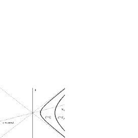
Figure 1: The $(x^{1},t)$ plane with the Rindler coordinates. The heavy lines $\xi=\xi_{1}$ and $\xi=\xi_{2}$ represent the trajectories of the plates.

To evaluate the VEV’s of the EMT by Eq. (2.3) we need the form of the eigenfunctions $\varphi_{\alpha}(x)$. For the geometry under consideration the metric and boundary conditions are static and translational invariant in the hyperplane parallel to the plates. It follows from here that the corresponding part of the eigenfunctions has the standard plane wave structure:

$$\varphi_{\alpha}=C\phi(\xi)\exp\left[i\left({\bf kx}-\omega\tau\right)\right],\quad\alpha=({\bf k},\omega),\quad{\mathbf{k}}=(k_{2},\ldots,k_{d}).$$ (2.7)

The equation for $\phi(\xi)$ is obtained from field equation (2.1) on background of metric (2.5) and has the form

$$\xi^{2}\phi^{\prime\prime}(\xi)+\xi\phi^{\prime}(\xi)+\left(\omega^{2}-k^{2}\xi^{2}\right)\phi(\xi)=0,$$ (2.8)

where the prime denotes a differentiation with respect to the argument, and $k=|{\bf k}|$. In the region between the plates the corresponding linearly independent solutions to equation (2.8) are the Bessel modified functions $I_{i\omega}(k\xi)$ and $K_{i\omega}(k\xi)$. The solution satisfying boundary condition (2.6) on the plate $\xi=\xi_{2}$ is in form

$$D_{i\omega}(k\xi,k\xi_{2})=I_{i\omega}(k\xi_{2})K_{i\omega}(k\xi)-K_{i\omega}(k\xi_{2})I_{i\omega}(k\xi).$$ (2.9)

Note that this function is real, $D_{i\omega}(k\xi,k\xi_{2})=D_{-i\omega}(k\xi,k\xi_{2})$. From the boundary condition on the plate $\xi=\xi_{1}$ we find that the possible values for $\omega$ are roots to the equation

$$D_{i\omega}(k\xi_{1},k\xi_{2})=0.$$ (2.10)

This equation has an infinite set of solutions. We will denote them by $\omega=\omega_{Dn}$, $\omega_{Dn}>0$, $n=1,2,\ldots$, and will assume that they are arranged in the ascending order $\omega_{Dn}<\omega_{Dn+1}$. The coefficient $C$ in formula (2.7) is determined from the standard Klein-Gordon orthonormality condition for the eigenfunctions which for metric (2.5) takes the form

$$\left(\varphi_{\alpha},\varphi_{\alpha^{\prime}}\right)=-i\int d{\mathbf{x}}\int_{\xi_{1}}^{\xi_{2}}\frac{d\xi}{\xi}\varphi_{\alpha}\stackrel{{\scriptstyle\leftrightarrow}}{{\partial}}_{\tau}\varphi^{*}_{\alpha^{\prime}}=\delta_{\alpha\alpha^{\prime}}.$$ (2.11)

It can be easily seen that for any two solutions to equation (2.8), $\phi_{\omega}^{(m)}(\xi)$, $m=1,2$ the following integration formula takes place

$$\int_{\xi_{1}}^{\xi_{2}}\frac{d\xi}{\xi}\phi_{\omega}^{(1)}(\xi)\phi_{v}^{(2)}(\xi)=\frac{\xi}{\omega^{2}-\upsilon^{2}}\left[\phi_{\omega}^{(1)}(\xi)\frac{d\phi_{\upsilon}^{(2)}(\xi)}{d\xi}-\phi_{\nu}^{(2)}(\xi)\frac{d\phi_{\omega}^{(1)}(\xi)}{d\xi}\right]_{\xi_{1}}^{\xi_{2}}.$$ (2.12)

Taking into account boundary condition (2.6) from Eq. (2.11) for the normalization coefficient one finds

$$C_{D}^{2}=\frac{1}{\left(2\pi\right)^{d-1}}\frac{I_{i\omega}(k\xi_{1})}{I_{i\omega}(k\xi_{2})\frac{\partial D_{i\omega}(k\xi_{1},k\xi_{2})}{\partial\omega}}\mid_{\omega=\omega_{Dn}}.$$ (2.13)

Now substituting the eigenfunctions

$$\varphi_{\alpha}^{D}(x)=C_{D}D_{i\omega_{Dn}}(k\xi,k\xi_{2})\exp\left[i\left({\bf kx}-\omega_{Dn}\tau\right)\right]$$ (2.14)

into Eq. (2.3) and integrating over the directions of $\ {\bf k}$ for the VEV’s of the EMT we obtain diagonal form (no summation over $i$)

$$\langle 0_{D}|T_{i}^{k}|0_{D}\rangle=\delta_{i}^{k}\pi A_{d}\int_{0}^{\infty}dkk^{d}\sum_{n=1}^{\infty}\frac{I_{i\omega}(k\xi_{1})}{I_{i\omega}(k\xi_{2})\frac{\partial D_{i\omega}(k\xi_{1},k\xi_{2})}{\partial\omega}}f^{(i)}[D_{i\omega}(k\xi,k\xi_{2})]\mid_{\omega=\omega_{Dn}},$$ (2.15)

where $|0_{D}\rangle$ is the amplitude for the Dirichlet vacuum between the plates, and

$$A_{d}=\frac{1}{2^{d-2}\pi^{(d+1)/2}\Gamma(\frac{d-1}{2})}.$$ (2.16)

In formula (2.15) for a given function $G(z)$ we use the notations

$$f^{(0)}[G(z)] = \left(\frac{1}{2}-2\zeta\right)\left|\frac{dG(z)}{dz}\right|^{2}+\frac{\zeta}{z}\frac{d}{dz}|G(z)|^{2}+\left[\frac{1}{2}-2\zeta+\frac{\omega^{2}}{z^{2}}\left(\frac{1}{2}+2\zeta\right)\right]|G(z)|^{2},$$ (2.17)

$$f^{(1)}[G(z)] = -\frac{1}{2}\left|\frac{dG(z)}{dz}\right|^{2}-\frac{\zeta}{z}\frac{d}{dz}|G(z)|^{2}+\frac{1}{2}\left(1-\frac{\omega^{2}}{z^{2}}\right)|G(z)|^{2},$$ (2.18)

$$f^{(i)}[G(z)] = -\frac{|G(z)|^{2}}{d-1}-\left(2\zeta-\frac{1}{2}\right)\left[\left|\frac{dG(z)}{dz}\right|^{2}+\left(1-\frac{\omega^{2}}{z^{2}}\right)|G(z)|^{2}\right];\quad i=2,\ldots,d,$$ (2.19)

where $G(z)=D_{i\omega}(z,k\xi_{2})$, and the indices 0,1 correspond to the coordinates $\tau$, $\xi$ respectively. It can be easily seen that for a conformally coupled scalar the EMT (2.15) is traceless.

For the further evolution of VEV’s (2.15) we will apply to the sum over $n$ summation formula (A) derived in Appendix A by making use of the generalized Abel-Plana formula [17]. This yields

$$\langle 0_{D}|T_{i}^{k}|0_{D}\rangle=A_{d}\delta_{i}^{k}\int_{0}^{\infty}dkk^{d}\int_{0}^{\infty}d\omega\,\left\{\frac{\sinh\pi\omega}{\pi}\,f^{(i)}[\tilde{D}_{i\omega}(k\xi,k\xi_{2})]-\frac{I_{\omega}(k\xi_{1})}{I_{\omega}(k\xi_{2})}\frac{F^{(i)}[D_{\omega}(k\xi,k\xi_{2})]}{D_{\omega}(k\xi_{1},k\xi_{2})}\right\},$$ (2.20)

where we have introduced the notation

$$\tilde{D}_{i\omega}(k\xi,k\xi_{2})=K_{i\omega}(k\xi)-\frac{K_{i\omega}(k\xi_{2})}{I_{i\omega}(k\xi_{2})}I_{i\omega}(k\xi),$$ (2.21)

and the functions $F^{(i)}[G(z)]$, $i=0,1,\ldots,d$ are obtained from the functions $f^{(i)}[G(z)]$ (see Eqs. (2.17)–(2.19)) replacing $\omega\rightarrow i\omega$:

$$F^{(i)}[G(z)]=f^{(i)}[G(z),\omega\rightarrow i\omega].$$ (2.22)

The vacuum energy density, $\varepsilon$, effective pressures in perpendicular, $p$, and parallel, $p_{\bot}$, to the plates directions are determined by relations (no summation over $i$)

$$\varepsilon=\langle 0_{D}|T_{0}^{0}|0_{D}\rangle,\quad p=-\langle 0_{D}|T_{1}^{1}|0_{D}\rangle,\quad p_{\bot}=-\langle 0_{D}|T_{i}^{i}|0_{D}\rangle,\quad i=2,\ldots,d.$$ (2.23)

It can be easily checked from Eqs. (2.20), (4.6) and (2.17)–(2.19) that they satisfy the standard continuity equation for the EMT, which for the geometry under consideration takes the form

$$\frac{d(\xi p)}{d\xi}=-\varepsilon.$$ (2.24)

For a conformally coupled scalar we have an additional zero–trace relation $\varepsilon-p-(d-1)p_{\perp}=0$. Let us consider the limit $\xi_{2}\rightarrow\infty$ of general formula (2.20) for fixed $\xi$. It can be easily seen that in this limit the VEV’s take the form

$$\lim_{\xi_{2}\rightarrow\infty}\langle 0_{D}|T_{i}^{k}|0_{D}\rangle=\langle 0_{R}|T_{i}^{k}|0_{R}\rangle+\langle T_{i}^{k}\rangle_{D}^{(1b)}(\xi_{1},\xi),\quad\xi>\xi_{1},$$ (2.25)

where

$$\langle 0_{R}|T_{i}^{k}|0_{R}\rangle=\frac{A_{d}\delta_{i}^{k}}{\pi}\int_{0}^{\infty}dkk^{d}\int_{0}^{\infty}d\omega\sinh\pi\omega\,f^{(i)}[K_{i\omega}(k\xi)]$$ (2.26)

are the corresponding VEV’s for the Fulling–Rindler vacuum without boundaries, and the term

$$\langle T_{i}^{k}\rangle_{D}^{(1b)}(\xi_{1},\xi)=-A_{d}\delta_{i}^{k}\int_{0}^{\infty}dkk^{d}\int_{0}^{\infty}d\omega\frac{I_{\omega}(k\xi_{1})}{K_{\omega}(k\xi_{1})}F^{(i)}[K_{\omega}(k\xi)]$$ (2.27)

is induced in the region $\xi>\xi_{1}$ by the presence of a single plane boundary located at $\xi=\xi_{1}$. Expressions (2.27) are finite for all values $\xi>\xi_{1}$ and all divergences are contained in the purely Fulling-Rindler part (2.26). These divergences can be regularized subtracting the corresponding VEV’s for the Minkowskian vacuum. The subtracted VEV’s

$$\langle T_{i}^{k}\rangle_{{\mathrm{sub}}}^{(R)}=\langle 0_{R}|T_{i}^{k}|0_{R}\rangle-\langle 0_{M}|T_{i}^{k}|0_{M}\rangle$$ (2.28)

are investigated in a large number of papers (see, for instance, [15, 16, 22, 23, 24, 25, 26, 27, 28, 29, 30, 31, 32] and references therein). The most general case of a massive scalar field in an arbitrary number of spacetime dimensions has been considered in Ref. [28] for conformally and minimally coupled cases and in Ref. [16] for general values of the curvature coupling parameter (for the corresponding Green function see [22]). The formulae relevant to this paper are given in [16]. For a massless scalar VEV’s (2.28) can be presented in the form

$$\langle T_{i}^{k}\rangle_{{\mathrm{sub}}}^{(R)}=-\frac{\delta_{i}^{k}\xi^{-d-1}}{2^{d-1}\pi^{d/2}\Gamma(d/2)}\int_{0}^{\infty}\frac{\omega^{d}g^{(i)}(\omega)d\omega}{e^{2\pi\omega}+(-1)^{d}}$$ (2.29)

(the expressions for the functions $g^{(i)}(\omega)$ are given in Ref. [16]) correspond to the absence from the vacuum of thermal distribution with standard temperature $T=(2\pi\xi)^{-1}$. As we see from Eq. (2.29), in general, the corresponding spectrum has non-Planckian form: the density of states factor is not proportional to $\omega^{d-1}d\omega$. The spectrum takes the Planckian form for conformally coupled scalars in $d=1,2,3$ with $g^{(0)}(\omega)=-dg^{(i)}(\omega)=1$, $i=1,2,\ldots d$. It is interesting to note that for even values of spatial dimension the distribution is Fermi-Dirac type (see also [33, 34]). For the massive scalar the energy spectrum is not strictly thermal and the corresponding quantities do not coincide with ones for the Minkowski thermal bath.

The boundary induced quantities (2.27) are investigated in Ref. [15] for a conformally coupled $d=3$ massless Dirichlet scalar and in Ref. [16] for a massive scalar with general curvature coupling and Robin boundary condition in an arbitrary number of dimensions. The single boundary part (2.27) diverges at the plate surface $\xi=\xi_{1}$ with leading terms proportional to $(\xi-\xi_{1})^{-d-1}$ for $i=0,2,\ldots,d$ and to $(\xi-\xi_{1})^{-d}$ for $i=1$ (see below). These leading terms vanish for a conformally coupled scalar, and for $i=0,2,\ldots,d$ coincide with the corresponding quantities for a plane boundary in the Minkowski vacuum [16].

Now we turn to the limit $\xi_{1}\rightarrow 0$ in formula (2.20), when the left plate coincides with the right Rindler horizon. In this limit in the second term on the right of formula (2.20) the subintegrand behaves as $\xi_{1}^{2\omega}$ and tends to zero. As a result one obtains

$$\lim_{\xi_{1}\rightarrow 0}\langle 0_{D}|T_{i}^{k}|0_{D}\rangle=\frac{A_{d}\delta_{i}^{k}}{\pi}\int_{0}^{\infty}dkk^{d}\int_{0}^{\infty}d\omega\,\sinh\pi\omega\,f^{(i)}[\tilde{D}_{i\omega}(k\xi,k\xi_{2})].$$ (2.30)

These quantities coincide with the corresponding ones induced in the region $\xi<\xi_{2}$ by a single plate at $\xi=\xi_{2}$. They are investigated in Ref. [16], where it has been shown that the VEV’s (2.30) can be presented in the form similar to Eq. (2.25):

$$\lim_{\xi_{1}\rightarrow 0}\langle 0_{D}|T_{i}^{k}|0_{D}\rangle=\langle 0_{R}|T_{i}^{k}|0_{R}\rangle+\langle T_{i}^{k}\rangle^{(1b)}_{D}(\xi_{2},\xi),\quad\xi<\xi_{2},$$ (2.31)

where the expressions for the boundary part $\langle T_{i}^{k}\rangle_{D}^{(1b)}(\xi_{2},\xi)$ in the region $\xi<\xi_{2}$ are obtained from formulae (2.27) by replacing (see Ref. [16])

$$I_{\omega}\rightarrow K_{\omega},\quad K_{\omega}\rightarrow I_{\omega},\quad\xi_{1}\rightarrow\xi_{2},\quad\xi_{2}\rightarrow\xi_{1}.$$ (2.32)

By using Eqs. (2.20),(2.30),(2.31) the parts in the VEV’s induced by the existence of boundaries,

$$\langle T_{i}^{k}\rangle^{(b)}_{D}=\langle 0_{D}|T_{i}^{k}|0_{D}\rangle-\langle 0_{R}|T_{i}^{k}|0_{R}\rangle,$$ (2.33)

can be written as

$$\langle T_{i}\rangle^{(b)}_{D}\left(\xi_{1},\xi_{2},\xi\right)=\langle T_{i}^{k}\rangle_{D}^{(1b)}\left(\xi_{2},\xi\right)-A_{d}\delta_{i}^{k}\int_{0}^{\infty}dk\,k^{d}\int_{0}^{\infty}d\omega\frac{I_{\omega}(k\xi_{1})}{I_{\omega}(k\xi_{2})}\frac{F^{(i)}[D_{\omega}(k\xi,k\xi_{2})]}{D_{\omega}(k\xi_{1},k\xi_{2})}.$$ (2.34)

In Appendix C we show that the VEV’s (2.20) can be also presented in the form (C.4). Substituting Eq. (C) into this formula, the boundary VEV’s can be also written in the form

$$\langle T_{i}^{k}\rangle^{(b)}_{D}\left(\xi_{1},\xi_{2},\xi\right)=\langle T_{i}^{k}\rangle^{(1b)}_{D}(\xi_{1},\xi)-A_{d}\delta_{i}^{k}\int_{0}^{\infty}dk\,k^{d}\int_{0}^{\infty}d\omega\frac{K_{\omega}(k\xi_{2})}{K_{\omega}(k\xi_{1})}\frac{F^{(i)}[D_{\omega}(k\xi,k\xi_{1})]}{D_{\omega}(k\xi_{1},k\xi_{2})}.$$ (2.35)

This expression is obtained from Eq. (2.34) by replacements (2.32). The case $d=1$ needs a separate consideration and is investigated in Appendix B. It can be seen that the corresponding formulae for the VEV’s are also obtained from the formulae given above in this section replacing

$$A_{d}\int_{0}^{\infty}dk\,k^{d-2}\rightarrow\frac{1}{\pi},\quad k\rightarrow 0.$$ (2.36)

Now let us present the VEV’s (2.20) in the form

$$\langle 0|T_{i}^{k}|0\rangle_{D}=\langle 0_{R}|T_{i}^{k}|0_{R}\rangle+\langle T_{i}^{k}\rangle^{(1b)}_{D}(\xi_{1},\xi)+\langle T_{i}^{k}\rangle^{(1b)}_{D}(\xi_{2},\xi)+\Delta\langle T_{i}^{k}\rangle_{D}(\xi_{1},\xi_{2},\xi),\quad\xi_{1}<\xi<\xi_{2},$$ (2.37)

where

$$\Delta\langle T_{i}^{k}\rangle_{D}=-A_{d}\delta_{i}^{k}\int_{0}^{\infty}dkk^{d}\int_{0}^{\infty}d\omega I_{\omega}(k\xi_{1})\left[\frac{F^{(i)}[D_{\omega}(k\xi,k\xi_{2})]}{I_{\omega}(k\xi_{2})D_{\omega}(k\xi_{1},k\xi_{2})}-\frac{F^{(i)}[K_{\omega}(k\xi)]}{K_{\omega}(k\xi_{1})}\right]$$ (2.38)

is the ’interference’ term. The surface divergences are contained in the single boundary parts and this term is finite for all values $\xi_{1}\leq\xi\leq\xi_{2}$. An equivalent formula for $\Delta\langle T_{i}^{k}\rangle_{D}$ is obtained from Eq. (2.38) by replacements (2.32). In the limit $\xi_{1}\to\xi_{2}$ expressions (2.38) are divergent and for small values of $\xi_{2}/\xi_{1}-1$ the main contribution comes from the large values of $\omega$. Introducing a new integration variable $x=k/\omega$ and replacing Bessel modified functions by their uniform asymptotic expansions for large values of the order (see Ref. [35]) at the leading order over $1/(\xi_{2}-\xi_{1})$ one receives (no summation over $i$)

$$\langle T_{i}^{i}\rangle^{(1b)}_{D}(\xi_{j},\xi) \sim \frac{d(\zeta_{c}-\zeta)\Gamma\left(\frac{d+1}{2}\right)}{2^{d}\pi^{(d+1)/2}|\xi-\xi_{j}|^{d+1}},\quad i=0,2,\ldots,d,$$ (2.39)

$$\langle T_{1}^{1}\rangle^{(1b)}_{D}(\xi_{j},\xi) \sim \langle T_{0}^{0}\rangle^{(1b)}_{D}(\xi_{j},\xi)\frac{\xi_{j}-\xi}{d\xi_{j}},\quad j=1,2$$ (2.40)

for the single boundary terms, and

$$\Delta\langle T_{0}^{0}\rangle_{D} \sim -\frac{1}{d}\Delta\langle T_{1}^{1}\rangle_{D}+\frac{(\zeta-\zeta_{c})(\xi_{2}-\xi_{1})^{-d-1}}{2^{2d-1}\pi^{d/2}\Gamma(d/2)}\times$$

$$\times\int_{0}^{\infty}\frac{dtt^{d}}{e^{t}-1}\left[\exp\left(t\frac{\xi_{1}-\xi}{\xi_{2}-\xi_{1}}\right)+\exp\left(t\frac{\xi-\xi_{2}}{\xi_{2}-\xi_{1}}\right)\right]$$

$$\Delta\langle T_{1}^{1}\rangle_{D} \sim \frac{d\zeta_{R}(d+1)\Gamma\left(\frac{d+1}{2}\right)}{(4\pi)^{(d+1)/2}(\xi_{2}-\xi_{1})^{d+1}},\quad\Delta\langle T_{i}^{i}\rangle_{D}\sim\Delta\langle T_{0}^{0}\rangle_{D},\quad i=2,3,\ldots,$$ (2.42)

for the ’interference’ terms. Here $\zeta_{R}(s)$ is the Riemann zeta–function. Expressions (2.39), (2), (2.42) coincide with the corresponding formulae for two parallel plates geometry in $d+1$ – dimensional Minkowski spacetime with separation $\xi_{2}-\xi_{1}$ (see Ref. [36] for the conformally coupled case and Ref. [18] for the general case of the curvature coupling parameter $\zeta$). Note that in the limit under consideration the ’interference’ term (2.42) for the vacuum perpendicular pressure dominates the single boundary induced terms, given by Eq. (2.40).

3 Interaction forces between the plates

Now we turn to the interaction forces between the plates. The vacuum force acting per unit surface of the plate at $\xi=\xi_{i}$ is determined by the ${}^{1}_{1}$–component of the vacuum EMT at this point. The corresponding effective pressures can be presented as a sum of two terms:

$$p_{D}^{(i)}=p_{D1}^{(i)}+p_{D{\rm(int)}}^{(i)},\quad i=1,2.$$ (3.1)

The first term on the right is the pressure for a single plate at $\xi=\xi_{i}$ when the second plate is absent. This term is divergent due to the well known surface divergences in the subtracted VEV’s. The second term on the right of Eq. (3.1),

$$p_{D{\rm(int)}}^{(i)}=-\langle T_{1}^{1}\rangle^{(1b)}_{D}(\xi_{j},\xi_{i})-\Delta\langle T_{1}^{1}\rangle_{D}(\xi_{1},\xi_{2},\xi_{i}),\quad i,j=1,2,\quad j\neq i$$ (3.2)

is the pressure induced by the presence of the second plate, and can be termed as an interaction force. For the plate at $\xi=\xi_{2}$ the interaction term is due to the second summand on the right of Eq. (2.20). Substituting into this term $\xi=\xi_{2}$ and using the Wronskian relation for the modified Bessel functions one has

$$p_{D{\rm(int)}}^{(2)}(\xi_{1},\xi_{2})=-\frac{A_{d}}{2\xi_{2}^{2}}\int_{0}^{\infty}dkk^{d-2}\int_{0}^{\infty}d\omega\frac{I_{\omega}(k\xi_{1})}{I_{\omega}(k\xi_{2})D_{\omega}(k\xi_{1},k\xi_{2})}.$$ (3.3)

By a similar way from Eq. (2.35) for the interaction term on the plate at $\xi=\xi_{1}$ we obtain

$$p_{D{\rm(int)}}^{(1)}(\xi_{1},\xi_{2})=-\frac{A_{d}}{2\xi_{1}^{2}}\int_{0}^{\infty}dkk^{d-2}\int_{0}^{\infty}d\omega\frac{K_{\omega}(k\xi_{2})}{K_{\omega}(k\xi_{1})D_{\omega}(k\xi_{1},k\xi_{2})}.$$ (3.4)

As the function $D_{\omega}(k\xi,k\xi_{2})$ is positive for $\xi_{1}<\xi_{2}$, interaction forces per unit surface (3.3) and (3.4) are always attractive. They are finite for all $\xi_{1}<\xi_{2}$, and do not depend on the curvature coupling parameter $\zeta$. In the limit $\xi_{1}\rightarrow\xi_{2}$ these forces diverge due the contribution from the large values $\omega$ and in this limit by introducing a new integration variable we can replace the Bessel modified functions by their uniform asymptotic expansions for large values of the order. At the leading order for the perpendicular vacuum pressures we obtain formula (2.42) which corresponds to the standard Casimir attraction force for two parallel plates in Minkowski vacuum.

From expressions (3.3) and (3.4) it follows that

$$p_{D{\rm(int)}}^{(2)}(\xi_{1},\xi_{2})>p_{D{\rm(int)}}^{(1)}(\xi_{1},\xi_{2}).$$ (3.5)

This can be proved by using that the function $z^{2}I_{\omega}(z)K_{\omega}(z)$ is monotonic increasing. The latter directly follows from the relations

$$\sqrt{1+\frac{(\omega+1)^{2}}{z^{2}}}-\frac{1}{z}<\frac{I^{\prime}_{\omega}(z)}{I_{\omega}(z)}<\sqrt{1+\frac{\omega^{2}}{z^{2}}}$$ (3.6)

$$\sqrt{1+\frac{(\omega+1)^{2}}{z^{2}}}+\frac{1}{z}>-\frac{K^{\prime}_{\omega}(z)}{K_{\omega}(z)}>\sqrt{1+\frac{\omega^{2}}{z^{2}}}.$$ (3.7)

The proof for the right inequalities in Eqs. (3.6),(3.7) is presented in Ref. [15]. The left inequalities are obtained from the recurrence relations for the Bessel modified functions. For instance, in the case of the function $I_{\omega}(z)$ one has:

$$\frac{I^{\prime}_{\omega}(z)}{I_{\omega}(z)}=\frac{I_{\omega+1}(z)}{I_{\omega}(z)}+\frac{\omega}{z}=\left[\frac{I^{\prime}_{\omega+1}(z)}{I_{\omega+1}(z)}+\frac{\omega+1}{z}\right]^{-1}+\frac{\omega}{z}>$$

$$>\left[\sqrt{1+\frac{(\omega+1)^{2}}{z^{2}}}+\frac{\omega+1}{z}\right]^{-1}+\frac{\omega}{z}=\sqrt{1+\frac{(\omega+1)^{2}}{z^{2}}}-\frac{1}{z},$$ (3.8)

where we have used the right inequality in Eq. (3.6). The left inequality in Eq. (3.7) can be proved in a similar way.

To see the monotonicity properties of functions (3.3) and (3.4) note that

$$\xi_{1}\frac{\partial p_{D{\rm(int)}}^{(1)}}{\partial\xi_{2}}=-\xi_{2}\frac{\partial p_{D{\rm(int)}}^{(2)}}{\partial\xi_{1}}=\frac{A_{d}}{2\xi_{1}\xi_{2}}\int_{0}^{\infty}dkk^{D-2}\int_{0}^{\infty}\frac{d\omega}{D_{\omega}^{2}(k\xi_{1},k\xi_{2})}.$$ (3.9)

It follows from here that for a fixed value of $\xi_{1}$ ($\xi_{2}$) the quantity $p_{D{\rm(int)}}^{(1)}$ ($p_{D{\rm(int)}}^{(2)}$) is monotonic increasing (decreasing) function on $\xi_{2}$ ($\xi_{1}$). By taking into account that both this quantities are negative we conclude that the modulus of the interaction force on the plate at $\xi_{1}$ ($\xi_{2}$) is monotonic decreasing (increasing) function on $\xi_{2}$ ($\xi_{1}$) for a fixed value of $\xi_{1}$ ($\xi_{2}$). From formula (3.3) it follows that

$$\xi_{i}\frac{\partial p_{D{\rm(int)}}^{(i)}}{\partial\xi_{i}}=-(d+1)p_{D{\rm(int)}}^{(i)}-\xi_{j}\frac{\partial p_{D{\rm(int)}}^{(i)}}{\partial\xi_{j}},\quad i,j=1,2,\quad i\neq j.$$ (3.10)

For $i=2$ the both terms on the right are positive and hence, the same is the case for the function on the left. Therefore for a fixed $\xi_{1}$ the function $p_{D{\rm(int)}}^{(2)}$ is monotonic increasing on $\xi_{2}$ and the modulus of the corresponding interaction force is monotonic decreasing function on $\xi_{2}$. In the case $i=1$ the terms on the right in this formula have different signs. For a fixed value of $\xi_{2}$ the function $p_{D{\rm(int)}}^{(1)}$ is monotonic increasing on $\xi_{1}$ near the horizon, $\xi_{1}\rightarrow 0$, and monotonic decreasing near the second plane, $\xi_{1}\rightarrow\xi_{2}$. It follows from here the modulus of the corresponding interaction force acting on the plate at $\xi_{1}$ has minimum for some intermediate value.

In the limit $\xi_{2}\gg\xi_{1}$, introducing in Eq. (3.3) a new integration variable $x=k\xi_{2}$, and making use the formula

$$I_{\omega}(y)=\left(\frac{y}{2}\right)^{\omega}\frac{1}{\Gamma(\omega)}\left[1+{\cal O}(y^{2})\right],\quad y=x\xi_{1}/\xi_{2},$$ (3.11)

and the standard relation between the functions $K_{\omega}$ and $I_{\pm\omega}$ one finds

$$p_{D{\rm(int)}}^{(2)}\approx-\frac{\pi^{2}A_{d}}{48\xi_{2}^{d+1}\ln^{2}(2\xi_{2}/\xi_{1})}\int_{0}^{\infty}\frac{dxx^{d-2}}{I_{0}^{2}(x)}\left[1+{\cal O}\left(\frac{\ln x}{\ln(2\xi_{2}/\xi_{1})}\right)\right].$$ (3.12)

The similar calculation for Eq. (3.4) yields

$$p_{D{\rm(int)}}^{(1)}\approx-\frac{\pi^{2}A_{d}}{24\xi_{2}^{d-1}\xi^{2}_{1}\ln^{3}(2\xi_{2}/\xi_{1})}\int_{0}^{\infty}\frac{dxx^{d-2}K_{0}(x)}{I_{0}(x)}\left[1+{\cal O}\left(\frac{\ln x}{\ln(2\xi_{2}/\xi_{1})}\right)\right].$$ (3.13)

We have carried out numerical evaluations for the interaction forces by making use of formulae (3.3) and (3.4). In Fig. 2 the corresponding results are presented for $\xi_{2}^{d+1}p_{D{\rm(int)}}^{(i)}$, $i=1,2$ in the case $d=3$ as functions on $\xi_{1}/\xi_{2}$.

Figure 2: The $d=3$ vacuum effective pressures determining the interaction forces between Dirichlet parallel plates, multiplied by $\xi^{4}_{2}$, $\xi^{4}_{2}p_{D{\rm(int)}}^{(1)}$ (curve a) and $\xi^{4}_{2}p_{D{\rm(int)}}^{(2)}$ (curve b) as functions of the ratio $\xi_{1}/\xi_{2}$.

4 VEV’s and the interaction forces for the Neumann scalar

In this section we will consider VEV’s for the EMT in the case of a scalar field satisfying the Neumann boundary condition on the plates $\xi=\xi_{1},\xi_{2}$:

$$\frac{\partial\varphi}{\partial\xi}|_{\xi=\xi_{1}}=\frac{\partial\varphi}{\partial\xi}|_{\xi=\xi_{2}}=0.$$ (4.1)

The corresponding scheme is similar to that given above for the Dirichlet case. The eigenfunctions to the field equation (2.1) have form (2.7) with

$$\phi(\xi)=N_{i\omega}(k\xi,k\xi_{2})=I_{i\omega}^{\prime}(k\xi_{2})K_{i\omega}(k\xi)-K_{i\omega}^{\prime}(k\xi_{2})I_{i\omega}(k\xi).$$ (4.2)

As in the Dirichlet case this function is real. From the boundary condition on the plate $\xi=\xi_{1}$ we obtain that the corresponding eigenfrequencies are solutions to the equation

$$N^{\prime}_{i\omega}(k\xi_{1},k\xi_{2})=I_{i\omega}^{\prime}(k\xi_{2})K_{i\omega}^{\prime}(k\xi_{1})-K_{i\omega}^{\prime}(k\xi_{2})I_{i\omega}^{\prime}(k\xi_{1})=0.$$ (4.3)

We will denote them by ${\omega=\omega_{Nn}}$, $n=1,2,...$ , arranged in the ascending order $\omega_{Nn}<\omega_{Nn+1}$. The normalization coefficient $C$ can be found from orthonormality condition (2.11) using integration formula (2.12):

$$C_{N}^{2}=\frac{1}{\left(2\pi\right)^{d-1}}\frac{I_{i\omega}^{\prime}(k\xi_{1})}{I_{i\omega}^{\prime}(k\xi_{2})\frac{\partial N_{i\omega}^{\prime}(k\xi_{1},k\xi_{2})}{\partial\omega}}|_{\omega=\omega_{Nn}}.$$ (4.4)

Substituting the eigenfunctions into the mode sum formula (2.3) one obtains

$$\langle 0_{N}|T_{i}^{k}|0_{N}\rangle=\pi A_{d}\delta_{i}^{k}\int_{0}^{\infty}dkk^{d}\sum_{n=1}^{\infty}\frac{I_{i\omega}^{\prime}(k\xi_{1})}{I_{i\omega}^{\prime}(k\xi_{2})\frac{\partial N_{i\omega}^{\prime}(k\xi_{1},k\xi_{2})}{\partial\omega}}f^{(i)}[N_{i\omega}(k\xi,k\xi_{2})]|_{\omega=\omega_{Nn}},$$ (4.5)

where $|0_{N}\rangle$ is the amplitude for the Neumann vacuum state between the plates, and the functions $f^{(i)}[G(z)]$ are defined in accordance with Eqs. (2.17)–(2.19). To sum the series over the eigenfrequencies $\omega_{Nn}$ we will apply the summation formula derived in Appendix A, Eq. (A). This yields

$$\langle 0_{N}|T_{i}^{k}|0_{N}\rangle=A_{d}\delta_{i}^{k}\int_{0}^{\infty}dkk^{d}\int_{0}^{\infty}d\omega\,\left\{\frac{\sinh\pi\omega}{\pi}\,f^{(i)}[\tilde{N}_{i\omega}(k\xi,k\xi_{2})]-\frac{I_{\omega}^{\prime}(k\xi_{1})}{I_{\omega}^{\prime}(k\xi_{2})}\frac{F^{(i)}[N_{\omega}(k\xi,k\xi_{2})]}{N^{\prime}_{i\omega}(k\xi_{1},k\xi_{2})}\right\},$$ (4.6)

with functions $F^{(i)}[G(z)]$ defined as in Eq. (2.22), and we use the notation

$$\tilde{N}_{\omega}(k\xi,k\xi_{2})=K_{i\omega}(k\xi)-\frac{K_{i\omega}^{\prime}(k\xi_{2})}{I_{i\omega}^{\prime}(k\xi_{2})}I_{i\omega}(k\xi).$$ (4.7)

To identify the terms in Eq. (4.6) let us consider limiting cases. In the limit $\xi_{2}\to\infty$, from Eq. (4.6) one obtains

$$\lim_{\xi_{2}\to\infty}\langle 0_{N}|T_{i}^{k}|0_{N}\rangle=\langle 0_{R}|T_{i}^{k}|0_{R}\rangle+\langle T_{i}^{k}\rangle^{(1b)}_{N}(\xi_{1},\xi),$$ (4.8)

where the term

$$\langle T_{i}^{k}\rangle^{(1b)}_{N}(\xi_{1},\xi)=-A_{d}\delta_{i}^{k}\int_{0}^{\infty}dkk^{d}\int_{0}^{\infty}d\omega\frac{I^{\prime}_{\omega}(k\xi_{1})}{K^{\prime}_{\omega}(k\xi_{1})}F^{(i)}[K_{\omega}(k\xi)]$$ (4.9)

is induced in the region $\xi>\xi_{1}$ by a single Neumann boundary located at $\xi=\xi_{1}$. This quantities for $d=3$ case are investigated in Ref. [15]. In the limit $\xi_{1}\to 0$ the left plate coincides with the Rindler horizon and the second term in the figure braces in Eq. (4.6) vanishes. In this case the VEV’s coincide with the corresponding expressions for a single plate at $\xi=\xi_{2}$ induced in the region $\xi<\xi_{2}$. They are investigated in Ref. [16], where it has been shown that the VEV’s (2.30) can be presented in the form similar to Eq. (4.8):

$$\lim_{\xi_{1}\to 0}\langle 0_{N}|T_{i}^{k}|0_{N}\rangle=\langle 0_{R}|T_{i}^{k}|0_{R}\rangle+\langle T_{i}^{k}\rangle^{(1b)}_{N}(\xi_{2},\xi),\quad\xi<\xi_{2},$$ (4.10)

where the expressions for the boundary part $\langle T_{Ni}^{\quad k}\rangle^{(1b)}_{N}(\xi_{2},\xi)$ in the region $\xi<\xi_{2}$ are obtained from formulae (4.9) by replacements (2.32).

By using Eqs. (4.6),(4.10) the parts in the VEV’s induced by the existence of boundaries,

$$\langle T_{i}^{k}\rangle^{(b)}_{N}=\langle 0_{N}|T_{i}^{k}|0_{N}\rangle-\langle 0_{R}|T_{i}^{k}|0_{R}\rangle,$$ (4.11)

can be presented as

$$\langle T_{i}^{k}\rangle^{(b)}_{N}\left(\xi_{1},\xi_{2},\xi\right)=\langle T_{i}^{k}\rangle^{(1b)}_{N}\left(\xi_{2},\xi\right)-A_{d}\delta_{i}^{k}\int_{0}^{\infty}dk\,k^{d}\int_{0}^{\infty}d\omega\frac{I^{\prime}_{\omega}(k\xi_{1})}{I^{\prime}_{\omega}(k\xi_{2})}\frac{F^{(i)}[N_{\omega}(k\xi,k\xi_{2})]}{N^{\prime}_{\omega}(k\xi_{1},k\xi_{2})}.$$ (4.12)

Similar to the Dirichlet case, the Neumann boundary VEV’s can be also written in the form

$$\langle T_{i}^{k}\rangle^{(b)}_{N}\left(\xi_{1},\xi_{2},\xi\right)=\langle T_{i}^{k}\rangle^{(1b)}_{N}(\xi_{1},\xi)-A_{d}\delta_{i}^{k}\int_{0}^{\infty}dk\,k^{d}\int_{0}^{\infty}d\omega\frac{K^{\prime}_{\omega}(k\xi_{2})}{K^{\prime}_{\omega}(k\xi_{1})}\frac{F^{(i)}[N_{\omega}(k\xi,k\xi_{1})]}{N^{\prime}_{\omega}(k\xi_{1},k\xi_{2})},$$ (4.13)

with $\langle T_{i}^{k}\rangle^{(1b)}_{N}(\xi_{1},\xi)$ being the VEV’s induced by a single Neumann boundary located at $\xi=\xi_{1}$. As we see, this expression is obtained from (4.12) by replacements (2.32).

Now let us present the VEV’s (4.6) in the form

$$\langle 0_{N}|T_{i}^{k}|0_{N}\rangle=\langle 0_{R}|T_{i}^{k}|0_{R}\rangle+\langle T_{i}^{k}\rangle^{(1b)}_{N}(\xi_{1},\xi)+\langle T_{i}^{k}\rangle^{(1b)}_{N}(\xi_{2},\xi)+\Delta\langle T_{i}^{k}\rangle_{N}(\xi_{1},\xi_{2},\xi),\quad\xi_{1}<\xi<\xi_{2},$$ (4.14)

where

$$\Delta\langle T_{i}^{k}\rangle_{N}=-A_{d}\delta_{i}^{k}\int_{0}^{\infty}dkk^{d}\int_{0}^{\infty}d\omega I^{\prime}_{\omega}(k\xi_{1})\left[\frac{F^{(i)}[N_{\omega}(k\xi,k\xi_{2})]}{I^{\prime}_{\omega}(k\xi_{2})N^{\prime}_{\omega}(k\xi_{1},k\xi_{2})}-\frac{F^{(i)}[K_{\omega}(k\xi)]}{K^{\prime}_{\omega}(k\xi_{1})}\right]$$

is the ’interference’ term. An equivalent formula for $\Delta\langle T_{i}^{k}\rangle_{N}$ is obtained from Eq. (4) by replacements (2.32).

’Interference’ term (4) is finite for all $\xi_{1}\leq\xi\leq\xi_{2}$, $\xi_{1}<\xi_{2}$, and diverges in the limit $\xi_{1}\to\xi_{2}$. In this limit the main contribution into the $\omega$–integral comes from the large values $\omega$. Introducing a new integration variable $x=k\xi_{1}/\omega$ and using the uniform asymptotic expansions for the Bessel modified functions in the leading order one obtains that the quantities $\Delta\langle T_{i}^{k}\rangle_{N}$ coincide with the VEV’s for two parallel plates in $d+1$–dimensional Minkowski spacetime with separation $\xi_{2}-\xi_{1}$ [36, 18]. The corresponding expressions are given by formulae (2),(2.42) with the opposite sign of the integral term on the right of formula (2).

Now we turn to the Neumann vacuum effective pressures determining the forces acting on the plate due to the presence of the second plate (interaction forces). This force acting per unit surface of the plate $\xi=\xi_{2}$, $p_{N{\mathrm{(int)}}}^{(2)}$ is defined by the ${}_{1}^{1}$–component of the second term on the right of formula (4.12) at $\xi=\xi_{2}$. The nonzero contribution comes from the last term on the right of Eq.(2.18) (with replacement (2.22)). Using the standard Wronskian relation for the Bessel modified functions one obtains

$$p_{N{\mathrm{(int)}}}^{(2)}(\xi_{1},\xi_{2})=\frac{A_{d}}{2\xi_{2}^{2}}\int_{0}^{\infty}dkk^{d-2}\int_{0}^{\infty}d\omega\frac{I^{\prime}_{\omega}(k\xi_{1})(1+\omega^{2}/k^{2}\xi_{2}^{2})}{I^{\prime}_{\omega}(k\xi_{2})N^{\prime}_{\omega}(k\xi_{1},k\xi_{2})}.$$ (4.15)

By a similar way for the interaction force per unit surface of the first plate from the second term on the right of Eq. (4.13) at $\xi=\xi_{1}$ we receive

$$p_{N{\mathrm{(int)}}}^{(1)}(\xi_{1},\xi_{2})=\frac{A_{d}}{2\xi_{1}^{2}}\int_{0}^{\infty}dkk^{d-2}\int_{0}^{\infty}d\omega\frac{K^{\prime}_{\omega}(k\xi_{2})(1+\omega^{2}/k^{2}\xi_{1}^{2})}{K^{\prime}_{\omega}(k\xi_{1})N^{\prime}_{\omega}(k\xi_{1},k\xi_{2})}.$$ (4.16)

Note that pressures (4.15),(4.16) are independent on the curvature coupling parameter. It can be seen that the function $I^{\prime}_{\omega}(z)/K^{\prime}_{\omega}(z)$ is monotonic decreasing, and as a result $N^{\prime}_{\omega}(k\xi_{1},k\xi_{2})<0$ for $\xi_{1}<\xi_{2}$. In combination with Eqs. (4.15), (4.16) it follows from here that $p_{N{\mathrm{(int)}}}^{(i)}<0$, $i=1,2$, and hence, as in the Dirichlet case, the Neumann interaction forces are always attractive. By using that the function $z^{4}I^{\prime}_{\omega}(z)K^{\prime}_{\omega}(z)/(z^{2}+\omega^{2})$ is monotonic decreasing (this can be proved by using inequalities (3.6),(3.7) ) we see that

$$p_{N{\mathrm{(int)}}}^{(2)}(\xi_{1},\xi_{2})>p_{N{\mathrm{(int)}}}^{(1)}(\xi_{1},\xi_{2}).$$ (4.17)

In the limit $\xi_{1}\to\xi_{2}$ replacing the Bessel modified functions by their uniform asymptotic expansions we can see that to the leading order from Eqs. (4.15),(4.16) the standard Casimir interaction force is obtained for two parallel plates with separation $\xi_{2}-\xi_{1}$ in the $d+1$–dimensional Minkowski spacetime.

From formulae (4.15), (4.16) one has

$$\xi_{1}\frac{\partial p_{N{\rm(int)}}^{(1)}}{\partial\xi_{2}}=-\xi_{2}\frac{\partial p_{N{\rm(int)}}^{(2)}}{\partial\xi_{1}}=\frac{A_{d}}{2\xi_{1}\xi_{2}}\int_{0}^{\infty}dkk^{D-2}\int_{0}^{\infty}d\omega\frac{(1+\omega^{2}/k^{2}\xi_{1}^{2})(1+\omega^{2}/k^{2}\xi_{2}^{2})}{N_{\omega}^{\prime 2}(k\xi_{1},k\xi_{2})}.$$ (4.18)

As seen from here for a fixed value of $\xi_{2}$ ($\xi_{1}$) the modulus of the interaction force acting on the plate at $\xi=\xi_{2}$ ($\xi_{1}$) is a monotonic increasing (decreasing) function on $\xi_{1}$ ($\xi_{2}$). For the other partial derivatives, similar to the Dirichlet case, one has the relation (3.10) with replacement $D\rightarrow N$. In particular, we can see that $\partial p_{N{\rm(int)}}^{(2)}/\partial\xi_{2}>0$. The Neumann effective pressures determining the interaction forces per unit surface given by Eqs. (4.15), (4.16) are plotted in Fig. 3 as functions of $\xi_{1}/\xi_{2}$ for the case $d=3$.

Figure 3: The $d=3$ vacuum effective pressures determining the interaction forces per unit surface between Neumann parallel plates, multiplied by $\xi^{4}_{2}$, $\xi^{4}_{2}p_{D{\rm(int)}}^{(1)}$ (curve a) and $\xi^{4}_{2}p_{D{\rm(int)}}^{(2)}$ (curve b) as functions of the ratio $\xi_{1}/\xi_{2}$.

As seen from Fig. 2 and Fig. 3 the Dirichlet and Neumann vacuum interaction forces are numerically close to each other. This is a consequence of that the subintegrands in formulae (3.3) and (4.15) and in formulae (3.4) and (4.16) are numerically close. This can be also seen analytically by using relations (3.6),(3.7).

5 Electromagnetic field

We now turn to the case of the electromagnetic field in the region $\xi_{1}<\xi<\xi_{2}$. We will assume that the mirrors are perfect conductors with the standard boundary conditions of vanishing of the normal component of the magnetic field and the tangential components of the electric field, evaluated at the local inertial frame in which the conductors are instantaneously at rest. By considerations similar to those given in Ref. [15] for $d=3$, it can be seen that the corresponding eigenfunctions for the vector potential $A^{\mu}$ may be resolved into one transverse magnetic (TM) and $d-2$ transverse electric (TE) (with respect to $\xi$-direction) modes $A^{\mu}_{\sigma\alpha}$, $\sigma=0,1,\ldots,d-2$, $\alpha=({\mathbf{k}},\omega)$:

$$A^{\mu}_{1\alpha} = \left(-\xi\partial/\partial\xi,-i\omega/\xi,0,\ldots 0\right)\varphi_{0\alpha},\quad\sigma=1,\quad{\mathrm{TM\,\,mode}},$$ (5.1)

$$A^{\mu}_{\sigma\alpha} = \epsilon^{\mu}_{\sigma}\varphi_{\sigma\alpha},\quad\sigma=0,2,\ldots,d-2,\quad{\mathrm{TE\,\,modes}},$$ (5.2)

where the polarization vectors $\epsilon^{\mu}_{\sigma}$ obey the following relations

$$\epsilon^{0}_{\sigma}=\epsilon^{1}_{\sigma}=0,\quad\epsilon_{\sigma\mu}\epsilon^{\mu}_{\sigma^{\prime}}=-k^{2}\delta_{\sigma\sigma^{\prime}},\quad\epsilon^{\mu}_{\sigma}k_{\mu}=0.$$ (5.3)

From the perfect conductor boundary conditions one has the following conditions for the scalar fields $\varphi_{\sigma\alpha}$:

$$\varphi_{\sigma\alpha}|_{\xi=\xi_{1}}=\varphi_{\sigma\alpha}|_{\xi=\xi_{2}}=0,\quad\sigma=0,2,\ldots,d-2,\quad\frac{\partial\varphi_{1\alpha}}{\partial\xi}|_{\xi=\xi_{1}}=\frac{\partial\varphi_{1\alpha}}{\partial\xi}|_{\xi=\xi_{2}}=0.$$ (5.4)

As a result the TE/TM modes correspond to the Dirichlet/Neumann scalars. In the corresponding expressions for the eigenfunctions $A^{\mu}_{\sigma\alpha}$ the normalization coefficient is determined from the orthonormality relation

$$\int d{\bf x}\int_{\xi_{1}}^{\xi_{2}}\frac{d\xi}{\xi}A_{\sigma\alpha}^{\mu}A_{\sigma^{\prime}\alpha^{\prime}\mu}^{\ast}=-\frac{2\pi}{\omega}\delta_{\alpha\alpha^{\prime}}\delta_{\sigma\sigma^{\prime}}.$$ (5.5)

On the base of this normalization condition for the separate scalar modes one has

$$\varphi_{\sigma\alpha}=\frac{2\pi^{1/2}}{k}C_{Z}Z_{i\omega_{Zn}}(k\xi,k\xi_{2})\exp\left[i\left({\bf kx}-\omega_{Zn}\tau\right)\right],$$ (5.6)

where $Z=D$ for $\sigma=0,2,\ldots,d-2$ and $Z=N$ for $\sigma=1$, and the coefficients $C_{D}$ and $C_{N}$ are defined in accordance with Eqs. (2.13),(4.4). Substituting the eigenfunctions (5.1), (5.2) into the mode sum formula

$$\langle 0|T_{i}^{k}|0\rangle=\sum_{\sigma=0}^{d-2}\int d{\bf k}\sum_{\omega_{Zn}}T_{i}^{k}\{A_{\sigma\alpha\mu},A_{\sigma\alpha\mu}^{\ast}\},$$ (5.7)

with the standard bilinear form for the electromagnetic field EMT one finds

$$\langle 0|T_{i}^{k}|0\rangle=\delta_{i}^{k}\frac{\pi^{(d-1)/2}}{\Gamma\left(\frac{d-1}{2}\right)}\int_{0}^{\infty}dk\,k^{d}\sum_{\sigma=0,1}\beta_{\sigma}\sum_{n=1}^{\infty}C_{Z}^{2}f_{{\mathrm{em}}}^{(i)}[Z_{i\omega_{Zn}}(k\xi,k\xi_{2})],\quad\beta_{0}=d-2,\quad\beta_{1}=1,$$ (5.8)

where $\beta_{0}$ and $\beta_{1}$ are the numbers of the independent polarization states for TE and TM modes respectively. In Eq. (5.8) for a given function $G(z)$ the following notations are introduced

$$f_{{\mathrm{em}}}^{(0)}[G(z)] = \left|\frac{dG(z)}{dz}\right|^{2}+\left(1+\frac{\omega^{2}}{z^{2}}\right)|G(z)|^{2},$$

$$f_{{\mathrm{em}}}^{(1)}[G(z)] = -\left|\frac{dG(z)}{dz}\right|^{2}+\left(1-\frac{\omega^{2}}{z^{2}}\right)|G(z)|^{2},$$ (5.9)

$$f_{{\mathrm{em}}}^{(i)}[G(z)] = \frac{d-5}{d-1}|G(z)|^{2}+\frac{d-3}{d-1}\left[\left|\frac{dG(z)}{dz}\right|^{2}-\frac{\omega^{2}}{z^{2}}|G(z)|^{2}\right],\quad i=2,3,\ldots,d.$$

By making use of the summation formulae derived in the Appendix A the VEV’s are presented in the form

$$\langle 0|T_{i}^{k}|0\rangle=\delta_{i}^{k}\frac{A_{d}}{2}\int_{0}^{\infty}dkk^{d}\int_{0}^{\infty}d\omega\sum_{\sigma=0,1}\beta_{\sigma}\left\{\frac{\sinh\pi\omega}{\pi}\,f_{{\mathrm{em}}}^{(i)}[\tilde{Z}_{i\omega}(k\xi,k\xi_{2})]-\frac{I_{\omega}^{(\sigma)}(k\xi_{1})F_{{\mathrm{em}}}^{(i)}[Z_{\omega}(k\xi,k\xi_{2})]}{I_{\omega}^{(\sigma)}(k\xi_{2})Z_{\omega}^{(\sigma)}(k\xi_{1},k\xi_{2})}\right\},$$ (5.10)

where $I_{\omega}^{(0)}=I_{\omega}$, $I_{\omega}^{(1)}=I^{\prime}_{\omega}$, and the same notations for the functions $K_{\omega}$, $Z_{\omega}$. The functions $F_{em}^{(i)}$ are obtained from Eqs. (5.9) replacing $\omega\rightarrow i\omega$:

$$F_{{\mathrm{em}}}^{(i)}[G(z)]=f_{{\mathrm{em}}}^{(i)}[G(z),\omega\rightarrow i\omega].$$ (5.11)

It can be easily checked that the components (5.10) obey the covariant conservation equation and the corresponding EMT is traceless for $d=3$. The first term in the figure braces of Eq. (5.10) corresponds to the VEV induced by a single plate at $\xi=\xi_{2}$ in the region $\xi<\xi_{2}$. For the case $d=3$ they are investigated in Ref. [16]. The generalization for an arbitrary $d$ is straightforward and these quantities are presented in the form

$$\langle 0|T_{i}^{k}|0\rangle^{(1b)}(\xi_{2},\xi)=\langle 0_{R}|T_{i}^{k}|0_{R}\rangle-\frac{1}{2}\delta_{i}^{k}A_{d}\int_{0}^{\infty}dkk^{d}\int_{0}^{\infty}d\omega\sum_{\sigma=0,1}\beta_{\sigma}\frac{K_{\omega}^{(\sigma)}(k\xi_{2})}{I_{\omega}^{(\sigma)}(k\xi_{2})}F_{{\mathrm{em}}}^{(i)}[I_{\omega}(k\xi)],$$ (5.12)

where $\langle 0_{R}|T_{i}^{k}|0_{R}\rangle$ are the VEV’s for the Fulling–Rindler electromagnetic vacuum without boundaries. By the way similar to that given in Ref. [16] for the case of a scalar field, it can be seen that

$$\langle 0_{R}|T_{i}^{k}|0_{R}\rangle=\langle 0_{M}|T_{i}^{k}|0_{M}\rangle-\frac{\delta_{i}^{k}(d-1)\xi^{-d-1}}{2^{d-1}\pi^{d/2}\Gamma(d/2)}\int_{0}^{\infty}\frac{\omega^{d}f_{0{\mathrm{em}}}^{(i)}(\omega)d\omega}{e^{2\pi\omega}+(-1)^{d}}\prod_{l=1}^{l_{m}}\left[\left(\frac{d-1-2l}{2\omega}\right)^{2}+1\right],$$ (5.13)

where $l_{m}=d/2-1$ for even $d>2$ and $l_{m}=(d-1)/2$ for odd $d>1$, and the value for the product over $l$ is equal to 1 for $d=1,2,3$. In Eq. (5.13) we have introduced notations

$$f_{0{\mathrm{em}}}^{(0)}(\omega) = -df_{0{\mathrm{em}}}^{(1)}(\omega)=1+\frac{(d-1)^{2}}{4\omega^{2}},$$ (5.14)

$$f_{0{\mathrm{em}}}^{(i)}(\omega) = f_{0{\mathrm{em}}}^{(1)}(\omega)+\frac{(d-1)(d-3)}{4\omega^{2}},\quad i=2,\ldots,d.$$

For physically most important case $d=3$, formula (5.13) leads to the standard result derived by Candelas and Deutsch in Ref. [15].

An alternative form for the vacuum EMT in the region between two plates is

$$\langle 0|T_{i}^{k}|0\rangle = \langle 0_{R}|T_{i}^{k}|0_{R}\rangle+\langle 0|T_{i}^{k}|0\rangle^{(1b)}(\xi_{1},\xi)-$$ (5.15)

$$- \frac{1}{2}\delta_{i}^{k}A_{d}\int_{0}^{\infty}dkk^{d}\int_{0}^{\infty}d\omega\sum_{\sigma=0,1}\beta_{\sigma}\frac{K_{\omega}^{(\sigma)}(k\xi_{2})F_{{\mathrm{em}}}^{(i)}[Z_{\omega}(k\xi,k\xi_{1})]}{K_{\omega}^{(\sigma)}(k\xi_{1})Z_{\omega}^{(\sigma)}(k\xi_{1},k\xi_{2})},$$

where $\langle 0|T_{i}^{k}|0\rangle^{(1b)}(\xi_{1},\xi)$ is the vacuum EMT induced by a single boundary at $\xi=\xi_{1}$ in the region $\xi>\xi_{1}$. The latter is obtained from (5.12) by replacements (2.32). For the interaction force $p^{(i)}_{{\mathrm{em(int)}}}$, $i=1,2$ per unit area of the plate at $\xi=\xi_{i}$ from Eqs. (5.10) and (5.15) one obtains

$$p^{(1)}_{{\mathrm{em(int)}}} = -\frac{A_{d}}{2\xi_{1}^{2}}\int_{0}^{\infty}dkk^{d-2}\int_{0}^{\infty}d\omega\sum_{\sigma=0,1}(-1)^{\sigma}\beta_{\sigma}\frac{K_{\omega}^{(\sigma)}(k\xi_{2})}{K_{\omega}^{(\sigma)}(k\xi_{1})}\frac{(1+\omega^{2}/k^{2}\xi_{1}^{2})^{\sigma}}{Z_{\omega}^{(\sigma)}(k\xi_{1},k\xi_{2})},$$ (5.16)

$$p^{(2)}_{{\mathrm{em(int)}}} = -\frac{A_{d}}{2\xi_{2}^{2}}\int_{0}^{\infty}dkk^{d-2}\int_{0}^{\infty}d\omega\sum_{\sigma=0,1}(-1)^{\sigma}\beta_{\sigma}\frac{I_{\omega}^{(\sigma)}(k\xi_{1})}{I_{\omega}^{(\sigma)}(k\xi_{2})}\frac{(1+\omega^{2}/k^{2}\xi_{2}^{2})^{\sigma}}{Z_{\omega}^{(\sigma)}(k\xi_{1},k\xi_{2})}.$$ (5.17)

Recalling that $(-1)^{\sigma}Z_{\omega}^{(\sigma)}>0$ we see the electromagnetic interaction forces are attractive. Note that $p^{(i)}_{{\mathrm{em(int)}}}=(d-2)p^{(i)}_{D{\mathrm{(int)}}}+p^{(i)}_{N{\mathrm{(int)}}}$. In the limit $\xi_{1}\to\xi_{2}$ and to the leading order over $1/(\xi_{2}-\xi_{1})$ from these expressions the electromagnetic Casimir interaction force between plates in the Minkowski spacetime is obtained.

6 Conclusion

It is well known that the uniqueness of vacuum state is lost when we work within the framework of quantum field theory in a general curved spacetime or in non–inertial frames. In this paper we have considered vacuum expectation values of the energy-momentum tensor for scalar and electromagnetic fields between two infinite parallel plates moving by uniform proper acceleration, assuming that the fields are prepared in the Fulling-Rindler vacuum state. As the boundaries are static in the Rindler coordinates no Rindler quanta are created and the only effect of the imposition of boundary conditions on quantum fields is the vacuum polarization. For the scalar case the both Dirichlet and Neumann boundary conditions are investigated. The VEV’s are presented in the form of mode sums involving series over zeros $\omega=\omega_{Dn}$ or $\omega=\omega_{Nn}$ of the functions $D_{i\omega}(k\xi_{1},k\xi_{2})$ and $N^{\prime}_{i\omega}(k\xi_{1},k\xi_{2})$ respectively. To sum these series we derive in Appendix A summation formulae for these types of series using the generalized Abel-Plana formula. The application of these formulae allows to extract from the VEV’s the parts due to the single plate. The latters are investigated previously in Refs. [15, 16]. The boundary induced parts are presented in two alternative forms, Eqs. (2.34), (2.35), for the Dirichlet case, and Eqs. (4.11),(4.12) for the Neumann case. Various limiting cases are studied. In particular, in the limit when the left plate coincides with the Rindler horizon the corresponding VEV’s are the same as for a single plate geometry. The vacuum forces acting on boundaries contain two terms. The first ones are the forces acting on a single boundary then the second boundary is absent. Due to the well–known surface divergences in the VEV’s of the energy-momentum tensor these forces are infinite and need an additional regularization. The another terms in the vacuum forces are finite and are induced by the presence of the second boundary and correspond to the interaction forces between the plates. These forces per unit surface do not depend on the curvature coupling parameter $\zeta$ and are determined by formulae (3.9),(3.10) for the Dirichlet scalar and by formulae (4.15),(4.16) for the Neumann scalar, and are always attractive for both plates. In particular, they are the same for conformally and minimally coupled scalars. For given $\xi_{1}$, $\xi_{2}$ the modulus of the interaction force is larger for the plate at $\xi=\xi_{1}$ (see inequalities (3.5) and (4.17)). For small distances between the plates at the leading order the standard Casimir result on background of the Minkowski vacuum is rederived. The case of the electromagnetic field is considered with the perfect conductor boundary conditions in the local inertial frame in which the boundaries are instantaneously at rest. The corresponding eigenmodes are superposition of TE and TM modes with Dirichlet and Neumann boundary conditions respectively. The VEV’s of the electromagnetic EMT in the region between the plates are given by formulae (5.10) and (5.15). The corresponding vacuum interaction forces per unit surface, Eqs. (5.16),(5.17), are obtained by summing the Dirichlet and Neumann $d=3$ scalar forces, and are attractive for all values of the proper accelerations for the plates.

The results obtained in this paper can be applied to the geometry of two parallel plates near the ’Rindler wall’. With the $x$ coordinate perpendicular to the wall and with the $(x^{2},x^{3})$ plane located at the centre of the wall, $x=0$, the static plane–symmetric line element can be written as

$$ds^{2}=e^{\nu(x)}dt^{2}-dx^{2}-e^{\lambda(x)}d{\mathbf{x}}^{2},\quad{\mathbf{x}}=(x^{2},x^{3}),$$ (6.1)

where $\nu(x)$ and $\lambda(x)$ are even functions. For this metric the Einstein equations with the diagonal matter energy-momentum tensor $T_{i}^{(m)k}={\mathrm{diag}}(\varepsilon^{(m)},-p^{(m)},-p^{(m)},-p^{(m)})$ admit two classes of solutions. For the first one $\lambda^{\prime}(0)>0$, and the corresponding external solution (the solution in the region $x>x_{s}$, where $T_{ik}^{(m)}=0$, with $x=x_{s}$ being the boundary of the wall) is described by the standard Taub metric [37]. For the second class of internal solutions $\lambda^{\prime}(0)<0$, and the external solution is presented by the metric

$$ds^{2}_{{\mathrm{ext}}}=e^{\nu_{s}}[1+2\pi\sigma_{s}(x-x_{s})]^{2}dt^{2}-dx^{2}-e^{\lambda_{s}}d{\mathbf{x}}^{2},$$ (6.2)

where $\nu_{s}=\nu(x_{s})$, $\lambda_{s}=\lambda(x_{s})$, and

$$\sigma_{s}=2e^{-\nu_{s}/2-\lambda_{s}}\int_{0}^{x_{s}}\left(\varepsilon^{(m)}+3p^{(m)}\right)e^{\nu/2+\lambda}dx$$ (6.3)

is the mass per unit surface of the wall. For a given equation of state $p^{(m)}=p^{(m)}(\varepsilon^{(m)})$ the parameters $\nu_{s},\lambda_{s},x_{s}$ are functions of the central pressure $p^{(m)}|_{x=0}$, and are determined by the internal solution of the Einstein equations (see Ref. [13] for the case of the equation of state corresponding to the incompressible liquid). Now redefining

$$\xi(x)=x-x_{s}+\frac{1}{2\pi\sigma_{s}},\quad\tau=2\pi\sigma_{s}e^{\nu_{s}/2}t,\quad e^{\lambda_{s}/2}x^{i}\to x^{i},\quad i=2,3,$$ (6.4)

from Eq. (6.2) we obtain the Rindler metric in the form (2.5). Hence, the VEV’s for the EMT in the region between two plates located at $x=x_{1}$ and $x=x_{2}$, $x_{i}>x_{s}$ near the ’Rindler wall’ are obtained from the results given above substituting $\xi_{i}=\xi(x_{i})$, $i=1,2$ and $\xi=\xi(x)$. Note that for $\sigma_{s}>0$, $x\geq x_{s}$ one has $\xi(x)\geq\xi(x_{s})>0$ and the Rindler metric is regular everywhere.

Appendix A Summation formulae over zeros of $D_{iz}$ and $N_{iz}^{\prime}$

In this section we will derive a summation formula over zeros $z=\omega_{Dk}$ of the function

$$D_{iz}(x,y)=I_{iz}(y)K_{iz}(x)-I_{iz}(x)K_{iz}(y),\quad y>x.$$ (A.1)

As we saw in section 2 the VEV’s of the EMT for the Dirichlet scalar between two plates in the Fulling-Rindler vacuum are expressed in the form of series over these zeros. To derive a summation formula we use the generalized Abel-Plana formula [17]. Let us choose in this formula

$$f(z) = \frac{2i}{\pi}\sinh\pi z\,F(z),$$ (A.2)

$$g(z) = \frac{I_{iz}(y)I_{-iz}(x)+I_{iz}(x)I_{-iz}(y)}{D_{iz}(x,y)}F(z),$$

with a meromorphic function $F(z)$ having poles $z=z_{k}$ in the right half-plane ${\rm Re}\,z\geq 0$. The sum and difference of functions (A.2) are presented in the form

$$g(z)\pm f(z)=\frac{2I_{\mp iz}(x)I_{\pm iz}(y)}{D_{iz}(x,y)}F(z).$$ (A.3)

By taking into account that the zeros $\omega_{Dk}$ are simple poles of the function $g(z)$ for the function $R[f(z),g(z)]$ in the generalized Abel-Plana formula one obtains

$$R[f(z),g(z)] = 2\pi i\left[\sum_{k=1}^{\infty}\frac{I_{-iz}(y)I_{iz}(x)}{\frac{\partial}{\partial z}D_{iz}(x,y)}F(z)|_{z=\omega_{Dk}}+\right.$$

$$+ \left.\sum_{k}{\rm Res}_{z=z_{k}}\frac{F(z)}{D_{iz}(x,y)}I_{i{\rm sgn}({\rm Im}z_{k})z}(y)I_{-i{\rm sgn}({\rm Im}z_{k})z}(x)\right],$$

where the zeros $\omega_{Dk}$ are arranged in ascending order. As a result we obtain the following summation formula

$$\sum_{k=1}^{\infty}\frac{I_{-iz}(y)I_{iz}(x)}{\frac{\partial}{\partial z}D_{iz}(x,y)}F(z)|_{z=\omega_{Dk}} = \frac{1}{\pi^{2}}\int_{0}^{\infty}\sinh\pi z\,F(z)dz-$$

$$- \sum_{k}{\rm Res}_{z=z_{k}}\frac{F(z)}{D_{iz}(x,y)}I_{i{\rm sgn}({\rm Im}z_{k})z}(y)I_{-i{\rm sgn}({\rm Im}z_{k})z}(x)-$$

$$- \frac{1}{2\pi}\int_{0}^{\infty}dz\frac{F(ze^{\pi i/2})+F(ze^{-\pi i/2})}{I_{-z}(y)K_{z}(x)-I_{-z}(x)K_{z}(y)}I_{z}(x)I_{-z}(y).$$

Here the condition for the function $F(z)$ is easily obtained from the corresponding condition in the Generalized Abel–Plana formula by using the asymptotic formulae for the Bessel modified function and has the form

$$|F(z)|<\epsilon(|z|)e^{-\pi z}\left(\frac{y}{x}\right)^{2|{\rm Im}z|},\quad{\rm Re\,}z>0,\quad|z|\rightarrow\infty,$$ (A.6)

where $|z|\epsilon(|z|)\rightarrow 0$ when $|z|\rightarrow\infty$.

A similar formula can be obtained for the series over zeros $z=\omega_{Nk}$, $k=1,2,\ldots$ of the function

$$N_{iz}^{\prime}(x,y)=I_{iz}^{\prime}(y)K_{iz}^{\prime}(x)-K_{iz}^{\prime}(y)I_{iz}^{\prime}(x),\quad\;y>x.$$ (A.7)

For this let us substitute in the Generalized Abel-Plana formula [17]

$$f(z) = \frac{2i}{\pi}\sinh\pi z\,F(z)$$ (A.8)

$$g(z) = \frac{I^{\prime}{}_{iz}(y)I^{\prime}{}_{-iz}(x)+I^{\prime}{}_{iz}(x)I^{\prime}{}_{-iz}(y)}{N_{iz}^{\prime}(x,y)}F(z).$$

Using these expressions it can bee easily seen that

$$g(z)\pm f(z)=\frac{2I_{\mp iz}^{\prime}(x)I_{\pm iz}^{\prime}(y)}{N_{iz}^{\prime}(x,y)}F(z).$$ (A.9)

For the function $R[f(z),g(z)]$ now one obtains

$$R[f(z),g(z)] = 2\pi i\left[\sum_{k=1}^{\infty}\frac{I^{\prime}{}_{-iz}(y)I^{\prime}{}_{iz}(x)}{\frac{\partial}{\partial z}N_{iz}^{\prime}(x,y)}F(z)|_{z=\omega_{Nk}}+\right.$$

$$+ \left.\sum_{k}{\rm Res}_{z=z_{k}}\frac{F(z)}{N_{iz}^{\prime}(x,y)}I_{i{\rm sgn}({\rm Im}z_{k})z}(y)I_{-i{\rm sgn}({\rm Im}z_{k})z}(x)\right].$$

As a result we obtain the following summation formula

$$\sum_{k=1}^{\infty}\frac{I^{\prime}{}_{-iz}(y)I^{\prime}{}_{iz}(x)}{\frac{\partial}{\partial z}N_{iz}^{\prime}(x,y)}F(z)|_{z=\omega_{Nk}} = \frac{1}{\pi^{2}}\int_{0}^{\infty}\sinh\pi z\,F(z)dz-$$

$$- \sum_{k}{\rm Res}_{z=z_{k}}\frac{F(z)}{N_{iz}^{\prime}(x,y)}I_{i{\rm sgn}({\rm Im}z_{k})z}(y)I_{-i{\rm sgn}({\rm Im}z_{k})z}(x)-$$

$$- \frac{1}{2\pi}\int_{0}^{\infty}dz\frac{F(ze^{\pi i/2})+F(ze^{-\pi i/2})}{I_{-z}^{\prime}(y)K_{z}^{\prime}(x)-I_{-z}^{\prime}(x)K_{z}^{\prime}(y)}I_{z}^{\prime}(x)I_{-z}^{\prime}(y),$$

where the corresponding condition for the function $F(z)$ has the form (A.6).

Appendix B $d=1$ case: Direct evoluation

For $d=1$ case the linearly independent solutions to equation (2.8) are $e^{\pm i\omega\ln\xi}$. The normalized eigenfunctions satisfying Dirichlet boundary conditions (2.6) are in form

$$\varphi_{n}^{D}=\frac{e^{-i\omega\tau}}{\sqrt{\pi n}}\sin(\alpha n),\quad\omega=\frac{\pi n}{\ln(\xi_{2}/\xi_{1})},\quad n=1,2,\ldots,$$ (B.1)

where we use the notation

$$\alpha=\frac{\pi\ln(\xi_{2}/\xi)}{\ln(\xi_{2}/\xi_{1})}.$$ (B.2)

Substituting eigenfunctions (B.1) into mode–sum formula (2.3) and applying to the sum over $n$ the Abel–Plana summation formula one finds

$$\langle 0_{D}|T_{i}^{k}|0_{D}\rangle-\langle 0_{M}|T_{i}^{k}|0_{M}\rangle = \langle T_{i}^{k}\rangle_{{\mathrm{(sub)}}}^{(R)}+\langle T_{i}^{k}\rangle^{(1b)}_{D}(\xi_{2},\xi)+\zeta\frac{\alpha^{2}/\sin^{2}\alpha-1}{2\pi\xi^{2}\ln^{2}(\xi_{2}/\xi)}{\mathrm{diag}}(1,0)-$$ (B.3)

$$- \frac{1}{2\pi\xi^{2}}\left[\frac{\pi^{2}}{12\ln^{2}(\xi_{2}/\xi_{1})}+\frac{\zeta}{\ln(\xi_{2}/\xi)}(\alpha\cot\alpha-1)\right]{\mathrm{diag}}(1,-1).$$

Here the subtracted purely Fulling–Rindler part without boundaries, $\langle T_{i}^{k}\rangle_{{\mathrm{(sub)}}}^{(R)}$, and the part induced by a single boundary at $\xi=\xi_{2}$ are given by formulae [16]

$$\langle T_{i}^{k}\rangle_{{\mathrm{(sub)}}}^{(R)}=\frac{1}{2\pi\xi^{2}}\left(\zeta-\frac{1}{12}\right){\mathrm{diag}}(1,-1),$$ (B.4)

$$\langle T_{i}^{k}\rangle^{(1b)}_{D}(\xi_{2},\xi)=\frac{\zeta}{2\pi\xi^{2}\ln(\xi/\xi_{2})}{\mathrm{diag}}(1+1/\ln(\xi/\xi_{2}),-1).$$ (B.5)

Note that the expression (B.5) for a single boundary part is valid for both regions $\xi<\xi_{2}$ and $\xi>\xi_{2}$. Now for the vacuum interaction forces between the plates one obtains

$$p_{D{\mathrm{(int)}}}^{(i)}=-\frac{\pi}{24\xi_{i}^{2}\ln^{2}(\xi_{2}/\xi_{1})},\quad i=1,2.$$ (B.6)

In the limit $\xi_{1}\to\xi_{2}$ to the leading order we recover the standard Casimir result on background of the 2D Minkowski spacetime.

For the case of the Neumann boundary conditions (4.1) the normalized eigenfunctions have the form

$$\varphi_{n}^{N}=\frac{e^{-i\omega\tau}}{\sqrt{\pi n}}\cos(\alpha n),\quad n=0,1,2,\ldots,$$ (B.7)

where $\omega$ and $\alpha$ are given by the same relations (B.1) and (B.2) as in the Dirichlet case. The substitution of these eigenfunctions into the mode–sum formula shows that the VEV’s of the EMT for the Neumann boundary conditions can be obtained from the corresponding formula for the Dirichlet case, Eq. (B.3), replacing in the boundary part $\zeta\to-\zeta$.

Appendix C Alternative representation for the VEV’s

As a solution to equation (2.8) satisfying first boundary condition (2.6) one could take the function

$$D_{i\omega}(k\xi,k\xi_{1})=I_{i\omega}(k\xi_{1})K_{i\omega}(k\xi)-K_{i\omega}(k\xi_{1})I_{i\omega}(k\xi).$$ (C.1)

Now from the boundary condition on the plate $\xi=\xi_{2}$ (2.6) we find the possible values for $\omega$ being roots to the equation (2.10). For the normalization coefficient we receive

$$C_{D}^{2}=\frac{1}{\left(2\pi\right)^{d-1}}\frac{I_{i\omega}(k\xi_{2})}{I_{i\omega}(k\xi_{1})\frac{\partial D_{i\omega}(k\xi_{1},k\xi_{2})}{\partial\omega}}|_{\omega=\omega_{Dn}}.$$ (C.2)

The VEV’s of the energy - momentum tensor are obtained in a diagonal form

$$\langle 0_{D}|T_{i}^{k}|0_{D}\rangle=\pi A_{d}\delta_{i}^{k}\int_{0}^{\infty}dkk^{d}\sum_{n=1}^{\infty}\frac{I_{i\omega}(k\xi_{2})}{I_{i\omega}(k\xi_{1})\frac{\partial D_{i\omega}(k\xi_{1},k\xi_{2})}{\partial\omega}}f^{(i)}[D_{i\omega}(k\xi,k\xi_{1})]|_{\omega=\omega_{Dn}}.$$ (C.3)

For the further evoluation of VEV’s (C.3) we can apply to the sum over $n$ summation formula (A). This gives

$$\langle 0_{D}|T_{i}^{k}|0_{D}\rangle = A_{d}\delta_{i}^{k}\int_{0}^{\infty}dkk^{d}\int_{0}^{\infty}d\omega\,\left\{\frac{\sinh\pi\omega}{\pi}f^{(i)}[\tilde{D}_{i\omega}(k\xi,k\xi_{1})]-\right.$$ (C.4)

$$-\left.\frac{I_{-\omega}(k\xi_{2})F^{(i)}[D_{\omega}(k\xi,k\xi_{1})]}{I_{-\omega}(k\xi_{1})D_{\omega}(k\xi_{1},k\xi_{2})}\right\}.$$

This form of the VEV’s is equivalent to Eq. (2.20). To see this let us consider the quantities

$$q_{j}^{(i)}=\frac{1}{\pi}\int_{0}^{\infty}d\omega\,\sinh\pi\omega\,f^{(i)}[\tilde{D}_{i\omega}(k\xi,k\xi_{j})]-\int_{0}^{\infty}d\omega\frac{I_{\omega}(k\xi_{1})I_{-\omega}(k\xi_{2})}{D_{\omega}(k\xi_{1},k\xi_{2})}\frac{F^{(i)}[D_{\omega}(k\xi,k\xi_{j})]}{I_{\omega}(k\xi_{j})I_{-\omega}(k\xi_{j})},$$ (C.5)

where $j=1,2$. Two representations (2.20) and (C.4) will be equivalent if

$$q_{1}^{(i)}=q_{2}^{(i)}.$$ (C.6)

To prove this let us consider the difference

$$q_{2}^{(i)}-q_{1}^{(i)}=\frac{1}{\pi}\int_{0}^{\infty}d\omega\,\sinh\pi\omega\,s^{(i)}-\int_{0}^{\infty}d\omega\frac{I_{\omega}(k\xi_{1})I_{-\omega}(k\xi_{2})}{D_{\omega}(k\xi_{1},k\xi_{2})}S^{(i)},$$ (C.7)

where we have introduced the notations

$$s^{(i)} = f^{(i)}[\tilde{D}_{i\omega}(k\xi,k\xi_{2})]-f^{(i)}[\tilde{D}_{i\omega}(k\xi,k\xi_{1})],$$ (C.8)

$$S^{(i)} = \sum_{j=1,2}(-1)^{j}\frac{F^{(i)}[D_{\omega}(k\xi,k\xi_{j})]}{I_{\omega}(k\xi_{j})I_{-\omega}(k\xi_{j})}.$$

By using the standard relation between the Bessel modified functions it can be seen that the first integral in formula (C.7) can be presented as

$$\frac{i}{2}\int_{0}^{\infty}\frac{I_{i\omega}(k\xi_{1})I_{-i\omega}(k\xi_{2})-I_{-i\omega}(k\xi_{1})I_{i\omega}(k\xi_{2})\,}{I_{i\omega}(k\xi_{2})K_{i\omega}(k\xi_{1})-I_{i\omega}(k\xi_{1})K_{i\omega}(k\xi_{2})}\,s^{(i)}d\omega,$$ (C.9)

where the function $s^{(i)}/(I_{i\omega}(k\xi_{2})K_{i\omega}(k\xi_{1})-I_{i\omega}(k\xi_{1})K_{i\omega}(k\xi_{2}))$ has no poles.  For the term with the first (second) summand in the numerator rotating the integration contour by angle $-\pi/2$ ($\pi/2$) in $\omega$ complex plane and noting that the integrals over arcs with large radius vanish (subintegrand behaves as $(\xi/\xi_{2})^{2|{\rm Im}\omega|}$) we see that

$$\frac{i}{2}\int_{0}^{\infty}\frac{I_{i\omega}(k\xi_{1})I_{-i\omega}(k\xi_{2})-I_{-i\omega}(k\xi_{1})I_{i\omega}(k\xi_{2})\,}{I_{i\omega}(k\xi_{2})K_{i\omega}(k\xi_{1})-I_{i\omega}(k\xi_{1})K_{i\omega}(k\xi_{2})}\,s^{(i)}d\omega=\int_{0}^{\infty}d\omega\frac{I_{\omega}(k\xi_{1})I_{-\omega}(k\xi_{2})}{D_{\omega}(k\xi_{1},k\xi_{2})}S^{(i)}.$$ (C.10)

Hence, the difference (C.7) is equal to zero, which directly proves Eq. (C.6)

By taking into account Eq. (C.5) from Eq. (C.6) in the limit $\xi_{2}\rightarrow\infty$ one obtains the following useful relation

$$\frac{1}{\pi}\int_{0}^{\infty}d\omega\,\sinh\pi\omega\,f^{(i)}[\tilde{D}_{i\omega}(k\xi,k\xi_{1})] = \frac{1}{\pi}\int_{0}^{\infty}d\omega\,\sinh\pi\omega\,f^{(i)}[K_{i\omega}(k\xi)]+$$

$$+\int_{0}^{\infty}d\omega\left\{\frac{F^{(i)}[D_{\omega}(k\xi,k\xi_{1})]}{I_{-\omega}(k\xi_{1})K_{\omega}(k\xi_{1})}-\frac{I_{\omega}(k\xi_{1})}{K_{\omega}(k\xi_{1})}F^{(i)}[K_{\omega}(k\xi]\right\}$$

Substituting Eq. (C) into Eq. (C.4) one finds formula (2.35).

References

• [1] H. B. G. Casimir, Proc. Kon. Nederl. Akad. Wet. 51, 793 (1948).
• [2] V. M. Mostepanenko and N. N. Trunov, The Casimir effect and its applications (Oxford University Press, Oxford, 1997).
• [3] G. Plunien, B. Muller and W.Greiner, Phys. Rep. 134, 87 (1986).
• [4] K. A. Milton, The Casimir Effect: Physical Manifestation of Zero–Point Energy (World Scientific, Singapore, 2002).
• [5] S. K. Lamoreaux, Am. J. Phys. 67, 850 (1999).
• [6] M. Bordag (Ed.), The Casimir Effect. 50 years later (World Scientific, Singapore, 1999).
• [7] M. Bordag, U. Mohidden, and V. M. Mostepanenko, Phys. Rep. 353, 1 (2001).
• [8] K. Kirsten, Spectral functions in Mathematics and Physics. CRC Press, Boca Raton, 2001.
• [9] S. A. Fulling, Phys. Rev D7, 2850 (1973).
• [10] S. A. Fulling, J. Phys. A: Math. Gen. 10, 917 (1977).
• [11] W. G. Unruh, Phys. Rev. D14, 870 (1976).
• [12] D. G. Boulware, Phys. Rev. D11, 1404 (1975).
• [13] R. M. Avakyan, E. V. Chubaryan, and A. H. Yeranyan, ”’Homogeneous’ gravitational field in General Relativity?”, gr-qc/0102030.
• [14] N. D. Birrell and P. C. W. Davies, Quantum fields in curved space (Chambridge University Press, Cambridge, England, 1982).
• [15] P. Candelas and D. Deutsch, Proc. Roy. Soc. Lond. A354, 79 (1977).
• [16] A. A. Saharian, ”Polarization of the Fulling–Rindler vacuum by a uniformly accelerated mirror”, hep-th/0110029.
• [17] A. A. Saharian, Izv. Akad. Nauk Arm. SSR. Matematika 22, 166 (1987)[Sov. J. Contemp. Math. Analysis. 22, 70 (1987)]; A. A. Saharian, ”The generalized Abel–Plana formula. Applications to Bessel functions and Casimir effect”, Report No. IC/2000/14; hep-th/0002239.
• [18] A. Romeo and A. A. Saharian, J. Phys. A: Math. Gen. 35, 1297 (2002).
• [19] A. Romeo and A. A. Saharian, Phys. Rev. D63, 105019 (2001).
• [20] A. A. Saharian, Phys. Rev. D63, 125007 (2001).
• [21] A. H. Rezaeian and A. A. Saharian, Local Casimir energy for a wedge with a circular outer boundary, hep-th/0110044, accepted for publication in Class. Quantum Grav.
• [22] P. Candelas and D. J. Raine, J. Math. Phys. 17, 2101 (1976).
• [23] P. C. Davies and S. Fulling, Proc. Roy. Soc. Lond. A345, 59 (1977).
• [24] P. Candelas and D. Deutsch, Proc. Roy. Soc. Lond. A362, 78 (1978).
• [25] W. Troost and H. van Dam, Nucl. Phys. B159, 442 (1979).
• [26] M. R. Brown and A. C. Ottewill, Phys. Rev. D31, 2514 (1985).
• [27] M. R. Brown, A. C. Ottewill, and D. Page, Phys. Rev. D33, 2840 (1986).
• [28] C. T. Hill, Nucl. Phys. B 277, 547 (1986).
• [29] V. P. Frolov and E. M. Serebriany, Phys. Rev. D35, 3779 (1987).
• [30] J. S. Dowker, Phys. Rev. D36, 3742 (1987).
• [31] R. Parentani, Class. Quantum Grav. 10, 1409 (1993).
• [32] V. Moretti and L. Vanzo, Phys. Lett. B375, 54 (1996).
• [33] S. Tagaki, Prog. Theor. Phys. 74, 142 (1985).
• [34] H. Ooguri, Phys. Rev. D33, 3573 (1986).
• [35] M. Abramowitz and I. A. Stegun, Handbook of Mathematical functions (National Bureau of Standards, Washington D.C.,1964).
• [36] J. Ambjørn and S. Wolfram, Ann. Phys. (N.Y.) 147, 1 (1983).
• [37] A. H. Taub, Ann. Math. 53, 472 (1951).