Perturbative – nonperturbative connection in quantum mechanics and field theory

Abstract

On the occasion of this ArkadyFest, celebrating Arkady Vainshtein’s $60^{\rm th}$ birthday, I review some selected aspects of the connection between perturbative and nonperturbative physics, a subject to which Arkady has made many important contributions. I first review this connection in quantum mechanics, which was the subject of Arkady’s very first paper. Then I discuss this issue in relation to effective actions in field theory, which also touches on Arkady’s work on operator product expansions. Finally, I conclude with a discussion of a special quantum mechanical system, a quasi-exactly solvable model with energy-reflection duality, which exhibits an explicit duality between the perturbative and nonperturbative sectors, without invoking supersymmetry.

I Divergence of perturbation theory

“The majority of nontrivial theories are seemingly unstable at some phase of the coupling constant, which leads to the asymptotic nature of the perturbative series.”   A. Vainshtein, 1964 arkady

In this talk I review some aspects of the historical development of the connection between perturbative and nonperturbative physics. It is particularly appropriate to look back on this subject on the occasion of Arkady Vainshtein’s $60^{\rm th}$ birthday, because this has been a central theme of many of Arkady’s great contributions to theoretical physics. In fact, in his very first physics paper arkady , now almost 40 years ago, Arkady made a fundamental contribution to this subject. This paper was published as a Novosibirsk report and so has not been widely circulated, especially in the West. For this ArkadyFest, Misha Shifman has made an English translation of this paper, and both the original Russian and the translation are reprinted in these Proceedings.

The physical realization of the possibility of the divergence of perturbation theory is usually traced back to a profound and influential paper by Dyson dyson , in which he argued that QED perturbation theory should be divergent. Dyson’s argument goes like this: a physical quantity in QED, computed using the standard rules of renormalized QED perturbation theory, is expressed as a perturbative series in powers of the fine structure constant, $\alpha=\frac{e^{2}}{4\pi}$:

$$F(e^{2})=c_{0}+c_{2}e^{2}+c_{4}e^{4}+\dots$$ (1)

Now, suppose that this perturbative expression is convergent. This means that in some small disc-like neighborhood of the origin, $F(e^{2})$ has a well-defined convergent approximation. In particular, this means that within this region, $F(-e^{2})$ also has a well-defined convergent expansion. Dyson then argued on physical grounds that this cannot be the case, because if $e^{2}<0$ the vacuum will be unstable. This, he argued, is because with $e^{2}<0$ like charges attract and it will be energetically favorable for the vacuum to produce $e^{+}e^{-}$ pairs which coalesce into like-charge blobs, a runaway process that leads to an unstable state:

“Thus every physical state is unstable against the spontaneous creation of large numbers of particles. Further, a system once in a pathological state will not remain steady; there will be a rapid creation of more and more particles, an explosive disintegration of the vacuum by spontaneous polarization.”   F. J. Dyson, 1952 dyson

The standard QED perturbation theory formalism breaks down in such an unstable vacuum, which Dyson argued means that $F(-e^{2})$ cannot be well-defined, and so the original perturbative expansion (1) cannot have been convergent.

Dyson’s argument captures beautifully an essential piece of physics, namely the deep connection between instability and the divergence of perturbation theory. The argument is not mathematically rigorous, and does not prove one way or another whether QED perturbation theory is convergent or divergent, or analytic or nonanalytic. However, it is nevertheless very suggestive, and has motivated many subsequent studies in both quantum mechanics and quantum field theory.

At roughly the same time, C. A. Hurst hurst and W. Thirring thirring (see also A. Petermann petermann ) showed by explicit computation that perturbation theory diverges in scalar $\phi^{3}$ theory. Both Hurst and Thirring found lower bounds on the contribution of Feynman graphs at a given order of perturbation theory, and showed that these lower bounds were themselves factorially divergent. Hurst used the parametric representation of an irreducible, renormalized and finite $\phi^{3}$ Feynman graph, to show that the magnitude of this graph was bounded below:

$$|I|\geq\frac{n^{-n+3/2-E/2}\,e^{2n-2}\,\pi^{-(n-E+5)/2}}{(2\pi)^{F}\,2^{n+1/2-3E/2}\,3^{4n-7/2}\,\gamma^{(n+E-4)/2}}\,\,\lambda^{n}$$ (2)

Here $n$ is the loop order, $\lambda$ is the cubic coupling constant, $E$ is the number of external lines, $F=\frac{1}{2}(3n-E)$ is the number of internal lines, and $\gamma$ is a constant depending on the external momenta. This lower bound is found by clever rearrangements of the parametric representation, together with the identity

$$\prod_{i=1}^{F}\left(\frac{1}{p_{i}^{2}+\kappa^{2}}\right)\geq\frac{F^{F}}{\left(\sum_{i=1}^{F}p_{i}^{2}+F\,\kappa^{2}\right)^{F}}$$ (3)

The second important piece of the argument is to show that there are no sign cancellations which would prevent this lower bound from a typical graph from being used to obtain a lower bound on the total contribution at a given order. This requires some technical caveats – for example, for a two-point function one requires $p^{2}<m^{2}$. The final piece of Hurst’s argument is the fact that the number of distinct Feynman diagrams at $n^{\rm th}$ loop order grows like $(\frac{n}{2})!\,n!$.

Together, the lower bound (2), the nonalternation of the sign, and the rapid growth of the number of graphs, lead to a lower bound for the total contribution at n-loop order (with E external lines):

$$\sum I\geq C^{n}\,n^{n/2+5/2-E/2}\,\lambda^{n}$$ (4)

Here $C$ is a finite constant, independent of $n$. Therefore, Hurst concluded that in $\lambda\phi^{3}$ theory, perturbation theory diverges for any coupling $\lambda$. He also suggests that a similar argument should hold for $\lambda\phi^{4}$ theory, and comments:

“If it be granted that the perturbation expansion does not lead to a convergent series in the coupling constant for all theories which can be renormalized, at least, then a reconciliation is needed between this and the excellent agreement found in electrodynamics between experimental results and low-order calculations. It is suggested that this agreement is due to the fact that the S-matrix expansion is to be interpreted as an asymptotic expansion in the fine-structure constant …”   C. A. Hurst, 1952 hurst

Thirring’s argument thirring was similar in spirit, although he concentrated on the $\phi^{3}$ self-energy diagram. Thirring found a set of graphs that were simple enough that their contribution could be estimated and bounded below, while plentiful enough that they made a divergent contribution to the perturbative series. He noted that the proof relied essentially on the fact that certain terms always had the same sign, and traced this fact to the hermiticity of the interaction. He found the following (weaker) lower bound, valid for $p^{2}<m^{2}$ :

$$\Delta(p^{2})\geq\sum_{n}C(p^{2})\,\left(\frac{\lambda\,e}{4\pi m3^{5/2}}\right)^{n}\,\frac{(\frac{n}{2}-2)!}{n^{2}}$$ (5)

Thirring concluded that there was no convergence for any $\lambda$. His final conclusion was rather pessimistic:

“To sum up, one can say that the chances for quantized fields to become a mathematically consistent theory are rather slender.”   W. Thirring, 1953 thirring

These results of Dyson, Hurst and Thirring, provide the backdrop for Arkady’s first paper arkady , “Decaying systems and divergence of perturbation theory”, written as a young student beginning his PhD at Novosibirsk. I encourage the reader to read Arkady’s paper – it is simple but deep. I paraphrase the argument here. The main contribution of his paper was to provide a quantitative statement of the relation between the divergence of perturbation theory and the unstable nature of the ground state in $\phi^{3}$ theory.

Motivated by the earlier results for $\phi^{3}$ theory (in 4 dimensions), Arkady had the clever idea to consider $\phi^{3}$ theory in $0+1$ dimensions, which is just quantum mechanics. Here it is natural to consider the hamiltonian

$$H=\frac{1}{2}\dot{\phi}^{2}+\frac{1}{2}m^{2}\phi^{2}-\lambda\phi^{3}$$ (6)

Figure 1: Unstable ground state for $V(\phi)=\frac{1}{2}\phi^{2}-\lambda\,\phi^{3}$

and the ground state $|\psi\rangle$ such that $H|\psi\rangle=E|\psi\rangle$. To make connection with the field theory results, note that the two-point function

$$i\,G(t)=\frac{\langle\psi|T\,\phi(t)\,\phi(0)\,|\psi\rangle}{\langle\psi|\psi\rangle}$$ (7)

is related to the energy $E$ as

$$i\,G(t=0)=\frac{1}{m}\,\frac{d\,E}{dm}=\frac{1}{m^{2}}\left(E-5\lambda^{2}\,\frac{dE}{d\lambda^{2}}\right)$$ (8)

where in the last step we have used the fact that, by dimensional reasoning, the energy $E$ can be expressed as $E=m\,f(\frac{\lambda^{2}}{m^{5}})$. Thus, if the perturbative expression for the two-point function diverges, the expression for the ground state energy, $E=E(\lambda^{2})$, should also diverge. One subtlety here is that the state $|\psi\rangle$ is clearly unstable. Arkady showed in an appendix arkady how to deal with this, by considering the adiabatic evolution of a stable state into an unstable state. In particular this suggests that the expression for $E=E(\lambda^{2})$ must have a cut along the positive $\lambda^{2}$ axis, as shown in Fig. 2, with an associated jump in the imaginary part of $E$ across this cut.

Figure 2: The complex $z=\lambda^{2}$ plane, showing the cut along the positive $z$-axis.

Under the (important) assumption that there are no other cuts or poles in the complex $z=\lambda^{2}$ plane, Cauchy’s theorem implies that :

$$E(z_{0}) = \frac{1}{2\pi i}\oint_{C}dz\,\frac{E(z)}{z-z_{0}}$$ (9)

$$= \frac{1}{\pi}\int_{0}^{R}dz\,\frac{Im\,E(z)}{z-z_{0}}$$

$$= \sum_{n=0}^{\infty}z_{0}^{n}\,\left(\frac{1}{\pi}\int_{0}^{R}dz\,\frac{Im\,E(z)}{z^{n+1}}\right)$$

Thus, the perturbative expansion coefficients are explicitly related to the moments of the imaginary part of the energy along the cut. Furthermore, it is clear from (9) that at large $n$ (i.e., at large order in perturbation theory), the dominant contribution comes from the behavior of $ImE(z)$ as $z\to 0$. This observation is very important, because the $z=\lambda^{2}\to 0$ limit is a semiclassical limit (note that the barrier height goes like $\frac{1}{\lambda^{2}}$, and the barrier width like $\frac{1}{\lambda}$). Hence, in this limit the imaginary part of the energy may be estimated using semiclassical techniques, such as WKB. Simple scaling shows that the leading WKB approximation for the imaginary part of the energy has the form

$$Im\,E(z)\sim\frac{a}{\sqrt{z}}\,e^{-b/z}\quad,\quad z\to 0$$ (10)

where $a$ and $b>0$ are (calculable) constants. Note, of course, that this expression is nonperturbative in $z=\lambda^{2}$.

Now consider the perturbative expansion for the lowest energy

$$E(\lambda^{2})=\frac{1}{2}+\sum_{n=1}c_{n}\lambda^{2n}$$ (11)

Inserting the WKB estimate (10) into the dispersion relation (9), we see that at large order the perturbation theory coefficients should behave as

$$c_{n}\sim\frac{a}{\pi}\int_{0}^{\infty}dz\,\frac{e^{-b/z}}{z^{n+3/2}}=\frac{a}{\pi}\,\frac{\Gamma(n+\frac{1}{2})}{b^{n+1/2}}$$ (12)

So, this argument suggests that the perturbative expansion (11) for $E(\lambda^{2})$ should be a divergent nonalternating series. Indeed, it is straightforward to do this perturbative calculation to very high orders, and to do the WKB calculation precisely, and one finds excellent agreement yaris . If the hamiltonian is rescaled as $H=p^{2}+\frac{1}{4}x^{2}-\lambda x^{3}$ (this scaling makes the expansion coefficients integers), then the leading growth rate for large $n$ is

$$c_{n}\sim-\frac{(60)^{n+1/2}}{(2\pi)^{3/2}}\,\,\Gamma(n+\frac{1}{2})\left[1-\frac{169}{60(2n-1)}+O\left(\frac{1}{n^{2}}\right)\right]$$ (13)

which agrees with Arkady’s form (12), and fits beautifully the growth rate of the actual expansion coefficients yaris . Indeed, the factorial growth of the perturbative coefficients kicks in rather early, as illustrated in Fig. 3.

The most important physics lessons from Arkady’s paper arkady are :

(i) the divergence of perturbation theory is related to the possible instability of the theory, at some phase of the coupling.

(ii) there is a precise quantitative relation (9) between the large-order divergence of the perturbative coefficients and nonperturbative physics.

Figure 3: The ratio of the exact perturbative coefficients $c_{n}$ in (11) to the leading WKB expression from (13), as a function of the order $n$.

In more modern language, this divergence associated with instability and tunneling is a divergence due to instantons. This idea has become a cornerstone of quantum field theory abc . However, since this time, it has been found that in quantum field theory (as distinct from quantum mechanics) there is yet another source of divergence in perturbation theory – this divergence is due to ”renormalons”, which arise essentially because of the running of the coupling constant, and can be related to special classes of diagrams thooft . For recent developments in this important subject, see the talks by M. Beneke, I. Balitsky and E. Gardi in these Proceedings.

The connection between the large-order behavior of quantum mechanical perturbation theory and WKB methods was developed independently, and was probed in great depth, by Bender and Wu, who studied the quartic anharmonic oscillator bw . Bender and Wu developed recursion techniques for efficiently generating very high orders of perturbation theory, and compared these results with higher orders of the WKB approximation. Their WKB analysis is a tour de force, and the agreement with the large order perturbative coefficients is spectacular.

Figure 4: Stable ground state for the potential $V=x^{2}+\lambda\,x^{4}$, on the left, and unstable ground state for the potential $V=x^{2}-\lambda\,x^{4}$, on the right.

The dependence of the ground state energy on the coupling $\lambda$ in the $\lambda\phi^{4}$ case is different from the $\lambda\phi^{3}$ case. As is clear from Fig. 4, in the $\lambda\phi^{4}$ case the instability arises when the coupling $\lambda$ changes sign from positive to negative. Thus, the cut is expected along the negative real axis in the complex $z=\lambda$ plane, which led Bender and Wu to the following dispersion relation:

$$c_{n}=\frac{1}{2\pi i}\int_{-\infty}^{0}\frac{dz}{z^{n}}\lim_{\epsilon\to 0}\left[F(z+i\epsilon)-F(z-i\epsilon)\right]$$ (14)

where $F(\lambda)=\frac{1}{\lambda}(E(\lambda)-\frac{1}{2})$ has one subtraction. Here, Bender and Wu made use of some rigorous results loeffel concerning the analyticity behavior of $E(\lambda)$ in the complex $\lambda$ plane : (i) $|E(\lambda)|\sim|\lambda|^{1/3}$ for large $|\lambda|$, (ii) $E(\lambda)$ is analytic in the cut $\lambda$-plane, with the cut along the negative real axis, and (iii) the expansion $E(\lambda)\sim\frac{1}{2}+\sum_{n=1}^{\infty}c_{n}\lambda^{n}$ is asymptotic.

The dispersion relation (14) relates the perturbative expansion coefficients for $F(\lambda)$ to the discontinuity of $F(\lambda$) across the cut. Bender and Wu used high orders of WKB to compute this nonperturbative imaginary part, thereby providing an extremely precise connection between the large orders of perturbation theory and semiclassical tunneling processes. They found that the expansion coefficients are alternating and factorially divergent

$$c_{n}=(-1)^{n+1}\frac{3^{n}\,\sqrt{6}\,\Gamma(n+\frac{1}{2})}{\pi^{3/2}}\left[1-\frac{95}{72n}+O\left(\frac{1}{n^{2}}\right)\right]$$ (15)

Bender and Wu extended these results to the general anharmonic oscillator:

$$\left(-\frac{d^{2}}{dx^{2}}+\frac{1}{4}x^{2}+\frac{\lambda}{2^{N}}\,x^{2N}-E(\lambda)\right)\psi=0$$ (16)

Then the $k^{\rm th}$ energy level has an asymptotic series expansion

$$E^{k,N}(\lambda)\sim k+\frac{1}{2}+\sum_{n=1}^{\infty}c_{n}^{k,N}\,\lambda^{n}$$ (17)

where the perturbative expansion coefficients $c_{n}^{k,N}$ are related to the lifetime of the $k^{\rm th}$ unstable level when the coupling $\lambda$ is negative:

$$c_{n}^{k,N}=\frac{(-1)^{n+1}(N-1)2^{k}\Gamma(nN-n+k+\frac{1}{2})}{\pi^{3/2}k!2^{n}}\left(\frac{\Gamma(\frac{2N}{N-1})}{\Gamma^{2}(\frac{N}{N-1})}\right)^{nN-n+\frac{1}{2}}\hskip-15.0pt\left[1+\dots\right]$$

(18)

Once again, these growth estimates are derived from WKB and fit the actual perturbative coefficients with great precision bw .

An important distinction between the $\lambda\phi^{3}$ and $\lambda\phi^{4}$ quantum mechanical oscillators is that the perturbative series for the energy eigenvalue is nonalternating in the $\lambda\phi^{3}$ case, and alternating in the $\lambda\phi^{4}$ case. This is directly related to the fact that the $\lambda\phi^{3}$ case is inherently unstable (for any real $\lambda$), while the $\lambda\phi^{4}$ case is stable if $\lambda>0$, but unstable if $\lambda<0$. Even though the quartic anharmonic oscillator with $\lambda>0$ is completely stable, the perturbative expression for the ground state energy is divergent, because the theory with $\lambda<0$ is unstable.

It is interesting to note that there has been much recent interest in certain nonhermitean hamiltonians, whose spectra appear to be completely real, despite the nonhermicity stefan . For example, there is very strong numerical evidence bdx3 ; bwen that the hamiltonian

$$H=p^{2}+\frac{1}{4}x^{2}+i\epsilon x^{3}$$ (19)

has a completely real spectrum. For the massless case, $H=p^{2}+i\epsilon x^{3}$, the reality of the spectrum has in fact been proved rigorously dorey . These results are nicely consistent with Arkady’s analysis of the $\lambda\phi^{3}$ quantum mechanical model, since an imaginary coupling corresponds to $z=\lambda^{2}$ being real and negative. In this region it was assumed that $E(z)$ is analytic (recall from Fig. 2 that the cut is along the positive $z$ axis), and the perturbative series is divergent but alternating, and can be analyzed using various standard (Padé and Borel) techniques bdx3 ; bwen , yielding excellent agreement with numerical integration results.

A useful mathematical technique for dealing with divergent series is Borel summation hardy ; bo ; zinnbook ; loeffel . This method is best illustrated by the paradigmatic case of the factorially divergent series. The series

$$f(g)\sim\sum_{n=0}(-1)^{n}\,n!\,g^{n}$$ (20)

is clearly divergent, and is alternating if $g>0$. Using the standard integral representation, $n!=\int_{0}^{\infty}ds\,e^{-s}s^{n}$, and formally interchanging the summation and integration, we can write

$$f(g)\sim\frac{1}{g}\int_{0}^{\infty}ds\,{e^{-s/g}\over 1+s}$$ (21)

This integral representation is defined to be the Borel sum of the divergent series in (20). The advantage of the integral is that it is convergent for all $g>0$. To be more precise, all this actually shows is that the integral in (21) has the same asymptotic series expansion as the divergent series in (20). In order for this identification between the series and the Borel integral to be unique, various further conditions must be satisfied hardy ; bo ; zinnbook . In some quantum mechanical examples it is possible to study these conditions rigorously loeffel , but unfortunately this is usually impossible in realistic quantum field theories. This means we are often confined to ”experimental mathematics” when applying Borel techniques to perturbation theory in QFT. Nevertheless, I prefer the attitude of Heaviside:

“The series is divergent; therefore we may be able to do something with it”   O. Heaviside, 1850 – 1925

to the (older) attitude of Abel:

“Divergent series are the invention of the devil, and it is shameful to base on them any demonstration whatsoever”   N. H. Abel, 1828

Continuing the paradigm in (20), when $g<0$ the series (20) becomes nonalternating. Then the same formal steps lead to the following representation:

$$f(-g)\sim\frac{1}{g}\int_{0}^{\infty}ds\,{e^{-s/g}\over 1-s}$$ (22)

Clearly there is a problem here, as there is a pole on the contour of integration, and so an ambiguity enters in the way one treats this pole. This means that the nonalternating factorially divergent series in (20), with $g<0$, is not Borel summable. For example, the principal parts prescription leads to the following imaginary part for the nonalternating series :

$$Imf(-g)=\frac{\pi}{g}\,\exp\left[-\frac{1}{g}\right]$$ (23)

This imaginary contribution is nonperturbative in the expansion parameter $g$. It is not seen at any finite order in perturbation theory. However, the imaginary part is inherently ambiguous in the absence of further physical information beyond the series expansion (20) itself.

Despite this ambiguity, it should be clear that the Borel approach provides a natural formalism with which to analyze the problem of the divergence of perturbation theory. It captures the essence of the connection with nonperturbative tunneling, and associates such nonperturbative effects with the unstable cases of the $\lambda\phi^{3}$ oscillator and the $\lambda\phi^{4}$ oscillator with $\lambda<0$, for which the perturbative series is indeed nonalternating and factorially divergent.

Similar formal expressions exist for the Borel sum of $f(g)\sim\sum c_{n}g^{n}$, if the $c_{n}$ are not simply factorial as in (20), but have the general form:

$$c_{n}\sim\beta^{n}\,\Gamma(\gamma\,n+\delta)$$ (24)

where $\beta$, $\gamma>0$ and $\delta$ are constants. Then the Borel sum approximation is

$$f(g)\sim\frac{1}{\gamma}\int_{0}^{\infty}\frac{ds}{s}\left(\frac{1}{1+s}\right)\left(\frac{s}{\beta g}\right)^{\delta/\gamma}\,\exp\left[-\left(\frac{s}{\beta g}\right)^{1/\gamma}\right]$$ (25)

For $g<0$ the nonalternating series has an imaginary part:

$$Im\,f(-g)\sim\frac{\pi}{\gamma}\left(\frac{1}{\beta g}\right)^{\delta/\gamma}\,\exp\left[-\left(\frac{1}{\beta g}\right)^{1/\gamma}\right]$$ (26)

In the next section we will use these relations in an explicit example.

Much more could be said about the divergence of perturbation theory, both in quantum mechanics and field theory. Lipatov lipatov generalized the instanton technique to scalar field theory, showing that large orders of perturbation theory may be described by pseudoclassical solutions of the classical field equations, together with quantum fluctuations. This approach built on instanton results of Langer langer in his classic study of metastability. Perturbation theory for systems with degenerate minima was investigated in degenerate , and a new twist on the perturbative–nonperturbative connection for this degenerate case is discussed in section 3 of this talk. For further references, I refer the interested reader to the review leguillou of Le Guillou and Zinn-Justin as an excellent source.

II Effective actions, OPEs, and divergent series

As mentioned previously, it is extremely difficult, even in quantum mechanics, to prove truly rigorous results concerning the divergence of perturbation theory loeffel ; in quantum field theory we are even more restricted when it comes to rigor. However, the study of effective actions is an example in QFT where some rigorous results are possible. This also makes connection with the subject of operator product expansions, which is another subject to which Arkady has made seminal contributions.

For this talk, I consider the QED effective action, which encodes nonlinear interactions due to quantum vacuum polarization effects, such as light-by-light scattering. The effective action is defined via the determinant that is obtained when the electron fields are integrated out of the QED functional integral:

$$S[A]=-\frac{i}{2}\log\det\left(D\hskip-6.0pt/^{2}+m^{2}\right)$$ (27)

where $D\hskip-6.0pt/=\gamma^{\mu}D_{\mu}=\gamma^{\mu}(\partial_{\mu}-ieA_{\mu})$ is the Dirac operator in the classical gauge field background $A_{\mu}$. The effective action has a natural perturbative expansion in terms of the electromagnetic coupling $e$, as represented in Fig. 5.

Figure 5: Perturbative expansion of the one-loop effective action

Indeed, by charge conjugation invariance (Furry’s theorem), the expansion involves only even numbers of external photon lines, which means that the perturbative series is actually a series in the fine structure constant $\alpha=\frac{e^{2}}{4\pi}$. Another natural expansion is the ”effective field theory” expansion (or ”large mass” expansion):

$$S[A]=m^{4}\sum_{n}\,c_{n}\,\frac{O^{(n)}}{m^{n}}$$ (28)

Here $O^{(n)}$ represents gauge invariant and Lorentz invariant terms constructed from the field strength $F_{\mu\nu}$, and having mass dimension $n$. For example, at mass dimension $8$, we can have $(F_{\mu\nu}F^{\mu\nu})^{2}$ or $(F_{\mu\nu}\tilde{F}^{\mu\nu})^{2}$, while at mass dimension $10$ we could have a term $(\partial_{\mu}F_{\nu\rho}\partial^{\mu}F^{\nu\rho})(F_{\alpha\beta}F^{\alpha\beta})$. As shown by Arkady and his collaborators arkadyope ; arkadyfs , such an expansion is related to the operator product expansion (OPE), such as that for

$$\Pi_{\mu\nu}=(q_{\mu}q_{\nu}-q^{2}g_{\mu\nu})\sum_{n}c_{n}(Q^{2})\,\langle O_{n}\rangle$$ (29)

In the special case where the classical background has constant field strength $F_{\mu\nu}$, the perturbative and large mass expansions coincide. This case of a constant background field was solved by Euler and Heisenberg euler (see also Weisskopf weisskopf and Schwinger schwinger ), who obtained an exact nonperturbative expression for the effective action:

$$S[A] = \frac{1}{8\pi^{2}}\int_{0}^{\infty}\frac{ds}{s^{3}}\,e^{-im^{2}s}\left\{(es)^{2}|{\mathcal{G}}|\cot\left[es\left(\sqrt{{\mathcal{F}}^{2}+{\mathcal{G}}^{2}}+{\mathcal{F}}\right)^{\frac{1}{2}}\right]\right.$$ (30)

$$\times\left.\,\coth\left[es\left(\sqrt{{\mathcal{F}}^{2}+{\mathcal{G}}^{2}}-{\mathcal{F}}\right)^{\frac{1}{2}}\right]-1+\frac{2}{3}(es)^{2}{\mathcal{F}}\right\}$$

Here ${\mathcal{F}}=\frac{1}{4}F_{\mu\nu}F^{\mu\nu}$, and ${\mathcal{G}}=\frac{1}{4}F_{\mu\nu}\tilde{F}^{\mu\nu}$, are the two Lorentz invariant combinations. The $-1$ term in the integrand corresponds to the zero-field subtraction of $S[0]$, while the last term, $\frac{2}{3}(es)^{2}{\mathcal{F}}$, corresponds to charge renormalization schwinger . There are several important physical consequences of this result euler ; weisskopf ; schwinger . First, expanding to leading order in the fields, we find the famous light-by-light term:

$$S=\frac{2\alpha^{2}}{45m^{4}}\int d^{4}x\,\left[(\vec{E}^{2}-\vec{B}^{2})^{2}+7(\vec{E}\cdot\vec{B})^{2}\right]+\dots$$ (31)

Second, for a constant electric field background, there is an imaginary part

$$Im\,S=\frac{e^{2}E^{2}}{8\pi^{3}}\sum_{k=1}^{\infty}\frac{1}{k^{2}}\,\exp\left[-\frac{k\,m^{2}\pi}{eE}\right]$$ (32)

which gives the pair production rate due to vacuum polarization.

The Euler-Heisenberg result (30) provides an excellent example of the application of Borel summation techniques, as we now review. Consider first of all the case of a uniform magnetic field background of strength $B$. Then the full perturbative expansion of the Euler-Heisenberg result is

$$S=-\frac{e^{2}B^{2}}{2\pi^{2}}\sum_{n=0}^{\infty}{{\mathcal{B}}_{2n+4}\over(2n+4)(2n+3)(2n+2)}\left(\frac{2eB}{m^{2}}\right)^{2n+2}$$ (33)

Viewed as a low energy effective action, the “low energy” condition here is simply that the characteristic energy scale for electrons in the magnetic background, $\hbar\frac{eB}{mc}$, is much smaller than the electron rest mass scale $mc^{2}$. The expansion coefficients in the series (33) involve the Bernoulli numbers ${\mathcal{B}}_{2n}$, which alternate in sign and grow factorially in magnitude abramowitz . Thus, the series (33) is an alternating divergent series. In fact, the expansion coefficients are:

$$c_{n} = {2^{2n}\,{\mathcal{B}}_{2n+4}\over(2n+4)(2n+3)(2n+2)}$$ (34)

$$= (-1)^{n+1}\,{\Gamma(2n+2)\over 8}\left[\frac{1}{\pi^{2n+4}}+\frac{1}{(2\pi)^{2n+4}}+\frac{1}{(3\pi)^{2n+4}}+\dots\right]$$

If we keep just the leading term in (34), then the expansion coefficients are of the form in (24), so that the Borel prescription (25) yields the leading Borel approximation for $S$ as

$$S_{\rm Borel}\sim{e^{2}B^{2}\over 4\pi^{6}}\int_{0}^{\infty}ds\,{s\over 1+s^{2}/\pi^{2}}\,\exp\left[-{m^{2}s\over eB}\right]$$ (35)

In Fig. 6 this leading Borel approximation is compared with successive terms from the perturbative expansion (33). Clearly the Borel representation is far superior for larger values of the expansion parameter $\frac{eB}{m^{2}}$.

Figure 6: Comparison of the leading Borel expression (35) [short-long-dash curve], as a function of $\frac{eB}{m^{2}}$, with the exact expression (36) [solid curve], and successive partial sums from the series (33) [short-dash curves]. The leading Borel expression is much better than the series expressions for $\frac{eB}{m^{2}}\geq 1$.

Actually, in this Euler-Heisenberg case, we can do even better since we are in the unusual situation of having the exact expression (34) for the perturbative coefficients, to all orders. Furthermore, the subleading terms in (34) are also of the form (24), for which we can once again use the Borel prescription (25). Including these subleading terms, we find

$$S=-{e^{2}B^{2}\over 8\pi^{2}}\int_{0}^{\infty}{ds\over s^{2}}\left(\coth s-{1\over s}-{s\over 3}\right)\,\exp\left[-{m^{2}s\over eB}\right]$$ (36)

where we have used the trigonometric expansion abramowitz :

$$\sum_{k=1}^{\infty}\frac{-2s^{3}}{k^{2}\pi^{2}(s^{2}+k^{2}\pi^{2})}=\coth s-\frac{1}{s}-\frac{s}{3}$$ (37)

It is interesting to note that the correct renormalization subtractions appear here. The integral representation (36) is precisely the Euler-Heisenberg expression (30), specialized to the case of a purely magnetic field. Thus, the ”proper-time” integral representation (36) is the Borel sum of the divergent perturbation series (33). Conversely, the divergent series (33) is the asymptotic expansion of the nonperturbative Euler-Heisenberg result (30).

Now consider the case of a purely electric constant background, of strength $E$. Perturbatively, the only difference from the constant magnetic case is that we replace $B^{2}\to-E^{2}$. This is because the only Lorentz invariant combination is $(E^{2}-B^{2})$ (clearly, $\vec{E}\cdot\vec{B}=0$ if one or other of $E$ or $B$ is zero). Thus, the alternating series in (33) becomes nonalternating, without changing the magnitude of the expansion coefficients. Applying the Borel dispersion relation (26) leads to an imaginary part in exact agreement with the nonperturbative pair-production result (32).

The divergence of the Euler-Heisenberg effective action is very well known ioffe ; og ; chadha ; pet ; zhitnitsky . This example is analogous to Dyson’s argument. The Euler-Heisenberg perturbative series cannot be convergent, because if it were convergent, then for very weak fields there would be no essential difference between the magnetic or electric background. However, we know from nonperturbative physics that there is an inherent vacuum instability in the case of an electric background, and that this leads to an exponentially small imaginary part to the effective action, which corresponds to pair production due to vacuum polarization.

The phenomenon of pair production from vacuum is fascinating, but is very difficult to observe because the exponential suppression factor is exceedingly small for realistic electric field strengths. The critical electric field at which the exponent becomes of order 1 is $E_{c}=\frac{m^{2}c^{3}}{e\hbar}\sim 10^{16}\,V/cm$, which is still several orders of magnitude beyond the peak fields obtained in the most intense lasers. See ringwald for a recent discussion of the prospects for observing vacuum pair production using an X-ray free-electron laser.

Even if one can produce such an intense background electric field, it is clear that it will not be a uniform field. Thus, it is important to ask how the Euler-Heisenberg analysis is modified when the background field is inhomogeneous. This is a very difficult problem in general. The most powerful approach is through semiclassical WKB techniques brezin ; popov . However, here I turn this question around and ask what this issue can tell us about the series expansion of the effective action when the background is inhomogeneous ted . If the field strength is inhomogeneous, then the large mass expansion (28) of the effective action involves many more terms at a given order, since we can now include terms involving derivatives of $F_{\mu\nu}$. In fact fleigner , the number of terms appears to grow factorially fast: 1, 2, 7, 36, … . But there are two obvious problems with quantifying this divergence. First, the expansion is not a true series, for the simple reason that at successive orders many completely new types of terms appear. Second, to learn anything nonperturbative one needs to go to very high orders in the derivative expansion, which is extremely difficult.

Fortunately, there is a special case in which both these problems are circumvented at once ted . Consider the particular inhomogeneous magnetic field pointing in the $z$-direction, but varying in the $x$-direction as:

$$\vec{B}(x)=\vec{B}\,{\rm sech}^{2}\left(x/\lambda\right)$$ (38)

where $\lambda$ is an arbitrary inhomogeneity scale. In such a background the effective action can be computed in closed-form using nonperturbative techniques dh1 . Also, since the inhomogeneity of the background is encoded solely in the dependence on the scale $\lambda$, the large mass expansion (28) can be expressed as a true series. That is, at a given order in the derivative expansion, all terms with the same number $d$ of derivatives combine to give a single contribution $\propto\frac{1}{(m\lambda)^{d}}$. Moreover, since this case is exactly soluble, we have access to all orders of the derivative expansion. Indeed, for the inhomogeneous magnetic background (38), the inverse mass expansion (28) becomes a double sum

$$\hskip-15.0ptS=-\frac{m^{4}}{8\pi^{3/2}}\sum_{j=0}^{\infty}\frac{1}{(m\lambda)^{2j}}\sum_{k=2}^{\infty}\left(\frac{2eB}{m^{2}}\right)^{2k}{\Gamma(2k+j)\Gamma(2k+j-2){\mathcal{B}}_{2k+2j}\over j!(2k)!\Gamma(2k+j+\frac{1}{2})}$$ (39)

with the two expansion parameters being the derivative expansion parameter, $\frac{1}{m\lambda}$, and the perturbative expansion parameter, $\frac{eB}{m^{2}}$. Note that the expansion coefficients are known to all orders, and are relatively simple numbers, just involving the Bernoulli numbers and factorial factors. It has been checked in dh1 that the first few terms of this derivative expansion are in agreement with explicit field theoretic calculations, specialized to this particular background.

Given the explicit series representation in (39), we can check that the series is divergent, but Borel summable. This can be done in several ways. One can either fix the order $k$ of the perturbative expansion in (39) and show that the remaining sum is Borel summable, or one can fix the order $j$ of the derivative expansion in (39) and show that the remaining sum is Borel summable. Or, one can sum explicitly the $k$ sum, for each $j$, as an integral of a hypergeometric function, and show that for various values of $\frac{eB}{m^{2}}$, the remaining derivative expansion is divergent but Borel summable. These arguments do not prove rigorously that the double series is Borel summable, but give a strong numerical indication that this is the case. It is interesting to note that an analogous double-sum structure also appears in the renormalon-OPE analysis in the talk by E. Gardi in these Proceedings.

It is also possible to compute the closed-form effective action for a time dependent electric field pointing in the $z$-direction:

$$\vec{E}(t)=\vec{E}\,{\rm sech}^{2}\left(t/\tau\right)$$ (40)

where $\tau$ characterizes the temporal inhomogeneity scale. A short-cut to the answer is to note that we can simply make the replacements, $B^{2}\to-E^{2}$, and $\lambda^{2}\to-\tau^{2}$, in the magnetic case result (39). In particular this has the consequence that the alternating divergent series of the magnetic case becomes a non-alternating divergent series, just as was found in the Euler-Heisenberg constant-field case. Fixing the order $j$ of the derivative expansion, the expansion coefficients behave for large $k$ (with $j$ fixed) as

$$\hskip-15.0ptc_{k}^{(j)}=\frac{(-1)^{j+k}\Gamma(2k+j)\Gamma(2k+j+2){\mathcal{B}}_{2k+2j+2}}{\Gamma(2k+3)\Gamma(2k+j+\frac{5}{2})}\sim 2{\Gamma(2k+3j-\frac{1}{2})\over(2\pi)^{2j+2k+2}}$$ (41)

Note that these coefficients are non-alternating and grow factorially with $2k$, as in the form of (24). Applying the Borel dispersion formula (26) gives

$$ImS^{(j)}\sim{m^{4}\over 8\pi^{3}}\left(\frac{eE}{m^{2}}\right)^{5/2}\,\exp\left[-\frac{m^{2}\pi}{eE}\right]\,\frac{1}{j!}\,\left({m^{4}\pi\over 4\tau^{2}e^{3}E^{3}}\right)^{j}$$ (42)

Remarkably, this form can be resummed in $j$, yielding a leading exponential

$$ImS\sim{m^{4}\over 8\pi^{3}}\left(\frac{eE}{m^{2}}\right)^{5/2}\,\exp\left[-\frac{m^{2}\pi}{eE}\left\{1-\frac{1}{4}\left(\frac{m}{eE\tau}\right)^{2}\right\}\right]$$ (43)

We recognize the first term in the exponent as the leading exponent in the constant field result (32). Thus, the second term may be viewed as the leading exponential correction to the constant-field answer (32). This is exactly what we set out to find, and we see that it arose through the divergence of the derivative expansion. I stress that this exponential correction is not accessible from low orders of the derivative expansion. This gives a Dyson-like argument that the derivative expansion must be divergent, since if it were not divergent, there would be no essential difference between the electric and magnetic cases, and there would be no correction to the exponent of the imaginary part of the effective action. However, we know, for example from WKB, that there is such a correction, and so the derivative expansion must be divergent.

In fact, the situation is even more interesting than the result (43) suggests. We could instead have considered doing the Borel resummation for the $j$ summations, at each fixed $k$. Then for large $j$, the coefficients go as

$$\hskip-15.0ptc_{j}^{(k)}=(-1)^{j+k}\frac{\Gamma(j+2k)\Gamma(j+2k-2){\mathcal{B}}_{2k+2j}}{\Gamma(j+1)\Gamma(j+2k+\frac{1}{2})}\sim 2^{\frac{9}{2}-2k}{\Gamma(2j+4k-\frac{5}{2})\over(2\pi)^{2j+2k}}$$ (44)

which once again are non-alternating and factorially growing. Applying the Borel dispersion formula (26) gives

$$ImS^{(k)}\sim{m^{3/2}\over 4\pi^{3}\tau^{5/2}}\,{(2\pi eE\tau^{2})^{2k}\over(2k)!}\,e^{-2\pi m\tau}$$ (45)

Once again, this leading form can be resummed, yielding

$$ImS\sim{m^{3/2}\over 8\pi^{3}\tau^{5/2}}\,\exp\left[-2\pi m\tau\left(1-\frac{eE\tau}{m}\right)\right]$$ (46)

Note that this leading exponential form of the imaginary part is different from that obtained in (43), and moreover, it is different from the constant-field case (32). The resolution of this puzzle is that there are two competing leading exponential behaviours buried in the double sum (39), and the question of which one dominates depends crucially on the relative magnitudes of the two expansion parameters, the derivative expansion parameter, $\frac{1}{m\tau}$, and the perturbative expansion parameter, $\frac{eE}{m^{2}}$. Another important quantity is their ratio, since this sets the scale of the corresponding gauge field:

$$\frac{A(t)}{m}=\frac{eE\tau\,{\rm tanh}(t/\tau)}{m}\sim\frac{eE\tau}{m}={eE/m^{2}\over 1/(m\tau)}$$ (47)

Thus, it is natural to define a “nonperturbative” regime, in which $\frac{eE\tau}{m}\gg 1$. Then $m\tau\gg\frac{m^{2}}{eE}$, so that the dominant exponential factor is $\exp[-\frac{m^{2}}{eE}]\gg\exp[-2\pi m\tau]$. In this regime, the leading imaginary contribution to the effective action is given by the expression (43), and we note that it is indeed nonperturbative in form, and the correction in the exponent is in terms of the small parameter $\frac{m}{eE\tau}\ll 1$. On the other hand, in the “perturbative” regime, where $\frac{eE\tau}{m}\ll 1$, this means that $m\tau\ll\frac{m^{2}}{eE}$, so that the dominant exponential factor is $\exp[-2\pi m\tau]\gg\exp[-\frac{m^{2}}{eE}]$. In this regime, the leading imaginary contribution to the effective action is given by the expression (46), and is in fact perturbative in nature, despite its exponential form.

These results are completely consistent with the WKB approach developed by Brézin and Itzykson brezin and Popov popov . For a time-dependent electric background $E(t)=\dot{A}_{z}(t)$, in the $z$-direction, the WKB expression for the imaginary part of the effective action is:

$$ImS\sim\int d^{3}k\,\exp[-\pi\Omega]$$ (48)

where $\Omega=\frac{2i}{\pi}\int_{\rm tp}\sqrt{m^{2}+k_{\perp}^{2}+(k_{z}-eA_{z}(t))^{2}}$. Applying this WKB analysis to the (exactly soluble) case $E(t)=E\,{\rm sech}^{2}(t/\tau)$, one obtains precisely the leading results (43) or (46), depending on whether we are in the “non-perturbative” $\frac{eE\tau}{m}\gg 1$, or “perturbative” $\frac{eE\tau}{m}\ll 1$ regime. This serves as a useful cross-check of the somewhat formal Borel analysis.

III Perturbative – nonperturbative duality in QES systems

In this last section I discuss some recent results ds concerning a new type of perturbative – nonperturbative connection that has been found in certain special quantum mechanical systems. We benefited from discussing these systems with Arkady, and I hope he enjoys the results!

Quasi-exactly solvable (QES) systems are those for which some finite portion of the energy spectrum can be found exactly using algebraic means itep . A positive integer parameter $J$ characterizes the ‘size’ of this exact portion of the spectrum. Two simple examples are : $V=x^{6}-(4J-1)x^{2}$, and $V=\sinh^{2}x-(2J-1)\cosh x$. For a QES system it is possible to define a quadractic form, $H=\sum_{a,b}c_{ab}J_{a}\,J_{b}+\sum_{a}d_{a}\,J_{a}$, in terms of $sl(2)$ generators of spin $J$, such that the eigenvalues of the algebraic matrix $H$ are the QES eigenvalues of the original system. It is interesting that algebraic hamiltonians of this form are widely used in the study of tunneling phenomena in single-molecule magnets magnet .

In bdm , the large $J$ limit of QES systems was identified as a semiclassical limit useful for studying the top of the quasi-exact spectrum. It was found that remarkable factorizations reduce the semiclassical calculation to simple integrals, leading to a straightforward asymptotic series representation for the highest QES energy eigenvalue. The notion of energy-reflection (ER) symmetry was introduced and analyzed in st2 : for certain QES systems the QES portion of the spectrum is symmetric under the energy reflection $E\leftrightarrow-E$. This means that for a system with ER symmetry, there is a precise connection between the top of the QES spectrum and the bottom of the spectrum. Coupled with the semiclassical large $J$ limit, the ER symmetry therefore relates semiclassical (nonperturbative) methods with perturbative methods st2 . In this section I discuss a class of periodic QES potentials for which the ER symmetry is in fact the fixed point (self-dual point) of a more general duality transformation. The duality between weak coupling and semiclassical expansions applies not just to the asymptotic series for the locations of the bands and gaps, but also to the exponentially small widths of bands and gaps.

Consider the quasi-exactly solvable (QES) Lamé equation ww :

$$\left\{-\frac{d^{2}}{d\phi^{2}}+J(J+1)\,\nu\,{\rm sn}^{2}(\phi|\nu)-\frac{1}{2}J(J+1)\right\}\Psi(\phi)=E\,\Psi(\phi)\,.$$ (49)

Here ${\rm sn}(\phi|\nu)$ is the doubly-periodic Jacobi elliptic function ww ; abramowitz , the coordinate $\phi\in R^{1}$, and $E$ denotes the energy eigenvalue. The real elliptic parameter $\nu$ lies in the range $0\leq\nu\leq 1$. The potential in (49) has period $2K(\nu)$, where $K(\nu)$ is the elliptic quarter period. The parameter $\nu$ controls the period of the potential, as well as its strength: see Fig. 7. As $\nu\to 1$, the period $2K(\nu)$ diverges logarithmically, $2K(\nu)\sim\ln\,(\frac{16}{1-\nu})$, while as $\nu\to 0$, the period tends to a nonzero constant: $2K(\nu)\to\pi$. In the Lamé equation (49), the parameter $J$ is a positive integer (for non-integer $J$, the problem is not QES). This parameter $J$ controls the depth of the wells of the potential; the constant subtraction $-\frac{1}{2}J(J+1)$ will become clear below.

Figure 7: The potential energy in (49) as a function of $\phi$, for $J=2$. The solid curve has elliptic parameter $\nu=0.95$, for which the period is $2K(0.95)\approx 5.82$. The dashed curve has $\nu=0.05$, for which the period is $2K(0.05)\approx 3.18$. Note how different the two potentials are; and yet, their spectra are related by the duality transformation (53).

It is a classic result that the Lamé equation (49) has bounded solutions $\Psi(\phi)$ with an energy spectrum consisting of exactly $J$ bands, plus a continuum band ww . It is the simplest example of a “finite-gap” model, there being just a finite number, $J$, of “gaps” in the spectrum. This should be contrasted with the fact that a generic periodic potential has an infinite sequence of gaps in its spectrum magnus . We label the band edge energies by $E_{l}$, with $l=1,2,\dots,(2J+1)$. Thus, the energy regions, $E_{2l-1}\leq E\leq E_{2l}$, and $E\geq E_{2l+1}$, are the allowed bands, while the regions, $E_{2l}<E<E_{2l+1}$, and $E<E_{1}$, are the gaps.

Another important classic result iachello ; ward concerning the Lamé model (49) is that the band edge energies $E_{l}$, for $l=1,\dots,2J+1$, are simply the eigenvalues of the finite dimensional $(2J+1)\times(2J+1)$ matrix

$$H=J_{x}^{2}+\nu J_{y}^{2}-\frac{1}{2}J(J+1)\,{\bf I}$$ (50)

where $J_{x}$ and $J_{y}$ are $su(2)$ generators in a spin $J$ representation and ${\bf I}$ is the unit matrix. Thus the Lamé band edge spectrum is algebraic, requiring only the finding of the eigenvalues of the finite dimensional matrix $H$ in (50). For example, for $J=1$ and $J=2$, the eigenvalues of $H$ are:

$$J=1\quad:\quad E_{1} = -1+\nu\,,$$

$$E_{2} = 0\,,$$

$$E_{3} = \nu\,;$$ (51)

$$J=2\quad:\quad E_{1} = -1+2\,\nu-2\,{\sqrt{1-\nu+\nu^{2}}}\,,$$

$$E_{2} = -2+\nu\,,$$

$$E_{3} = -2+4\,\nu\,,$$

$$E_{4} = 1+\nu\,,$$

$$E_{5} = -1+2\,\nu+2\,{\sqrt{1-\nu+\nu^{2}}}\,.$$ (52)

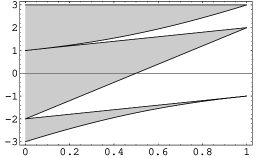
Figure 8: The energy bands (52) for the $J=2$ Lamé system (49), as a function of the elliptic parameter $\nu$. The shaded areas on this plot are the bands, while the unshaded areas are the gaps. The top band actually continues up to $E\to\infty$.

The spectrum of the Lamé system (49) has a special duality:

$$E[\nu]=-E[1-\nu]$$ (53)

That is, the spectrum of the Lamé system (49), with elliptic parameter $\nu$, is the energy reflection of the spectrum of the Lamé system with the dual elliptic parameter $1-\nu$. In particular, for the band edge energies, $E_{l}$, which are the eigenvalues of the finite dimensional matrix $H$ in (50), this means

$$E_{l}[\nu]=-E_{2J+2-l}\,[1-\nu]\qquad,\quad l=1,2,\dots,2J+1$$ (54)

This duality can be seen directly in the eigenvalues of the $J=1$ and $J=2$ examples in (51) and (52). The proof of the duality (54) for the band edge energies is a trivial consequence of the algebraic realization (50), since

$$J_{x}^{2}+\nu J_{y}^{2}-\frac{1}{2}J(J+1)\,{\bf I}=-\left[\left(J_{z}^{2}+(1-\nu)J_{y}^{2}\right)-\frac{1}{2}J(J+1)\,{\bf I}\right]$$ (55)

Noting that $[J_{z}^{2}+(1-\nu)J_{y}^{2}]$ has the same eigenvalues as $[J_{x}^{2}+(1-\nu)J_{y}^{2}]$, the duality result (54) follows. It is instructive to see this duality in graphical form, in Fig. 8, which shows the band spectra as a function of $\nu$. The transformation $\nu\to 1-\nu$, with the energy reflection $E\to-E$, interchanges the shaded regions (bands) with the unshaded regions (gaps). The fixed point, $\nu=\frac{1}{2}$, is the “self-dual” point, where the system maps onto itself; here the energy spectrum has an exact energy reflection (ER) symmetry.

In fact, the duality relation (53) applies to the entire spectrum, not just the band edges (54). This is a consequence of Jacobi’s imaginary transformation abramowitz . Making the coordinate transformation

$$\phi^{\prime}=i\left(\phi-K-i\,K^{\prime}\right)\,,$$ (56)

the Lamé equation (49) transforms into

$$\left\{-\frac{d^{2}}{d\phi^{\prime 2}}+J(J+1)\,(1-\nu)\,{\rm sn}^{2}(\phi^{\prime}|1-\nu)-\frac{1}{2}J(J+1)\right\}\Psi(\phi^{\prime})=-E\,\Psi(\phi^{\prime})$$

(57)

So solutions of (49) are mapped to solutions of the dual equation (57), with $\nu\to 1-\nu$, and with a sign reflected energy eigenvalue: $E\to-E$.

Figure 9: Contour plots in the $\phi$ plane of the real (left) and imaginary (right) parts of the potential function $sn^{2}(\phi|\nu)$, for $\nu=\frac{1}{2}$. Note that the potential is real along the real $\phi$ axis, and along the line $Re(\phi)=K(\frac{1}{2})\approx 1.85$ (as well as the periodic displacements). This corresponds to the rotation (56).

To see why bands and gaps are interchanged under our duality transformation (56), recall that the independent solutions of the original Lamé equation (49) can be written as products of theta functions ww , and under the change of variables (56), these theta functions map into the same theta functions, but with dual elliptic parameter. However, they map from bounded to unbounded solutions (and vice versa), because of the “i” factor appearing in (56). Thus, the bands and gaps become interchanged.

As an aside, I mention that the Lamé system plays a distinguished role in the theory of $su(2)$ BPS monopoles. For example, Ward has shown ward that the Lamé equation factorizes, using the Nahm equations (which are fundamental to the construction of monopole solutions)

$$\frac{dT_{j}}{ds}=\mp\frac{i}{2}\epsilon_{jkl}\,[T_{k},T_{l}]$$ (58)

To see this, define the quaternionic operators

$$\Delta_{\pm}={\bf 1}_{2n}\frac{d}{ds}\pm T_{j}(s)\otimes\sigma_{j}$$ (59)

where $T_{j}(s)$, for $j=1,2,3$, take values in an $n$-dimensional represenation of the Lie algebra $su(2)$. Then

$$\Delta_{\pm}\Delta_{\mp}=\left({\bf 1}_{n}\frac{d^{2}}{ds^{2}}-T_{j}T_{j}\right)\otimes{\bf 1}_{2}+\left(\mp\frac{dT_{j}}{ds}-\frac{i}{2}\epsilon_{jkl}\,[T_{k},T_{l}]\right)\otimes\sigma_{j}$$ (60)

and this combination is real if $T_{j}$ satisfy the Nahm equations (58). Furthermore, using the solution $T_{1}=-\sqrt{\nu}\,{\rm sn}(s)\,t_{1}$, $T_{2}=i\sqrt{\nu}\,{\rm cn}(s)\,t_{2}$, $T_{3}=i\,{\rm dn}(s)\,t_{3}$, where $t_{j}$ are $su(2)$ generators, it follows from properties of the elliptic functions that

$$T_{j}T_{j}=(t_{1}^{2}+t_{2}^{2}+t_{3}^{2})\,\nu\,{\rm sn}^{2}(s)-(\nu\,t_{2}^{2}+t_{3}^{2})$$ (61)

Thus, (60) provides a factorization of the Lamé operator. Subsequently, Sutcliffe showed sutcliffe that the spectral curve for the Nahm data for a charge $n=2j+1$ $su(2)$ monopole is related to a $j$-gap Lamé operator, and corresponds physically to $2j+1$ monopoles aligned along an axis.

Returning to the perturbative–nonperturbative duality (53), I first discuss how this operates for the locations of the bands and gaps in the Lamé spectrum. The location of a low-lying band can be calculated using perturbative methods, while the location of a high-lying gap can be calculated using semiclassical methods. The exact duality (53) between the top and bottom of the spectrum provides an explicit mapping between these two sectors. Defining $\kappa=\sqrt{J(J+1)}$, we see that $1/\kappa$ is the weak coupling constant of the perturbative expansion. Simultaneously, $1/\kappa$ plays the role of $\hbar$ in the quasiclassical expansion.

In the limit $J\to\infty$, the width of the lowest band becomes very narrow, so it makes sense to estimate the “location” of the band. In fact, the width shrinks exponentially fast, so we can estimate the location of the band to within exponential accuracy using elementary perturbation theory. A straightforward calculation ds shows that the lowest energy level is

$$E_{0}=-\frac{1}{2}\,\kappa^{2}\left[1-\frac{2\sqrt{\nu}}{\kappa}+\frac{\nu+1}{2\,\kappa^{2}}+\frac{(1-4\nu+\nu^{2})}{8\,\sqrt{\nu}\,\kappa^{3}}+O\left(\frac{1}{\kappa^{4}}\right)\right]\,.$$ (62)

We now consider the semiclassical evaluation of the location of the highest gap, in the limit $J\to\infty$. First, note that for a given $\nu$, as $J\to\infty$ the highest gap lies above the top of the potential. Thus, the turning points lie off the real $\phi$ axis. For a periodic potential the gap edges occur when the discriminant magnus takes values $\pm 1$. By WKB, the discriminant is

$$\Delta(E)=\cos\left(\frac{1}{\hbar}\,\,\sum_{n=0}^{\infty}\,\hbar^{n}\,S_{n}\,(P)\right)\,,$$ (63)

where $P$ is the period, and $S_{n}(x)$ are the standard WKB functions which can be generated to any order by a simple recursion formula bo . The $J^{\rm th}$ gap occurs when the argument of the cosine in the discriminant (63) is $J\pi$:

$$\kappa\,\,\sum_{n=0}^{\infty}\,\frac{1}{\kappa^{n}}\,{S_{n}\,(2K)}=J\,\pi=\pi\,\kappa\left(1-\frac{1}{2\,\kappa}+\frac{1}{8\,\kappa^{2}}-\frac{1}{128\,\kappa^{4}}+\dots\right)$$ (64)

where $2K$ is the period of the Lamé potential, and where on the right-hand side we have expressed $J$ in terms of the effective semiclassical expansion parameter $1/\kappa$. This relation (64) can be used to find an expansion for the energy of the $J^{\rm th}$ gap by expanding

$$E=\frac{1}{2}\,\kappa^{2}+\sum_{\ell=1}^{\infty}\,\frac{\varepsilon_{\ell}}{\kappa^{\ell-2}}\,.$$ (65)

The expansion coefficients $\varepsilon_{l}$ are fixed by identifying terms on both sides of the expansion in (64). A straightforward calculation ds leads to

$$E=\frac{1}{2}\,\kappa^{2}-\kappa\,\sqrt{1-\nu}+\frac{2-\nu}{4}+\frac{(-2+2\nu+\nu^{2})}{16\,\kappa\,\sqrt{1-\nu}}+\dots\,.$$ (66)

Comparing with the perturbative expansion (62) we see that the semiclassical expansion (66) is indeed the dual of the perturbative expansion (62), under the duality transformation $\nu\to 1-\nu$ and $E\to-E$.

This illustrates the perturbative – nonperturbative duality for the locations of bands and gaps. However, it is even more interesting to consider this duality for the widths of bands and gaps, because the calculations of widths are sensitive to exponentially small contributions which are neglected in the calculations of the locations.

The width of a low-lying band can be computed in a number of ways. First, since the band edge energies are given by the eigenvalues of the finite dimensional matrix $H$ in (50), the most direct way to evaluate the width of the lowest-lying band is to take the difference of the two smallest eigenvalues of $H$. This leads dr to the exact leading behavior, in the limit $\nu\to 1$, of the width of the lowest band, for any $J$ :

$$\Delta E^{\rm algebraic}_{\rm band}={8J\,\Gamma(J+1/2)\over 4^{J}\sqrt{\pi}\,\Gamma(J)}\,(1-\nu)^{J}\,\left(1+\frac{J-1}{2}(1-\nu)+\dots\right)$$ (67)

This clearly shows the exponentially narrow character of the lowest band.

In the instanton approximation, tunneling is suppressed because the barrier height is much greater than the ground state energy of any given isolated “atomic” well. The instanton calculation for the Lamé potential can be done in closed form dr , leading in the large $J$ and $\nu\to 1$ limit to

$$\Delta E^{\rm instanton}_{\rm band}\sim\frac{8J^{3/2}}{\sqrt{\pi}\,4^{J}}\,\,\left(1-\nu\right)^{J}\left[1+\frac{J-1}{2}(1-\nu)+\dots\right]\,,$$ (68)

which agrees perfectly with the large $J$ limit of the exact algebraic result (67). Thus, this example gives an analytic confirmation that the instanton approximation gives the correct leading large $J$ behavior of the width of the lowest band, as $\nu\to 1$.

Having computed the width of the lowest band by several different techniques, both exact and nonperturbative, we now turn to a perturbative evaluation of the width of the highest gap. First, taking the difference of the two largest eigenvalues of the finite dimensional matrix $H$ in (50), it is straightforward to show that as $\nu\to 0$, for any $J$, this difference gives

$$\Delta E^{\rm algebraic}_{\rm gap}={8J\,\Gamma(J+1/2)\over 4^{J}\sqrt{\pi}\,\Gamma(J)}\,\nu^{J}\left(1+\frac{J-1}{2}\,\nu+\dots\right)\,,$$ (69)

which is the same as the algebraic expression (67) for the width of the lowest band, with the duality replacement $\nu\to 1-\nu$. But it is more interesting to try to find this result from perturbation theory. From (69) we see that the width of the highest gap is of $J^{\rm th}$ order in perturbation theory. So, to compare with the semi-classical (large $J$) results for the width of the lowest band, we see that we will have to be able to go to very high orders in perturbation theory. This provides a novel, and very direct, illustration of the connection between nonperturbative physics and high orders of perturbation theory.

It is generally very difficult to go to high orders in perturbation theory, even in quantum mechanics. For the Lamé system (49) we can exploit the algebraic relation to the finite-dimensional spectral problem (50). However, since $H$ in (50) is a $(2J+1)\times(2J+1)$ matrix, the large $J$ limit is still non-trivial. Nevertheless, the high degree of symmetry in the Lamé system means that the perturbative calculation can be done to arbitrarily high order ds . The result is that the splitting between the two highest eigenvalues arises at the $J^{\rm th}$ order in perturbation theory, and is given by

$$\Delta E^{\rm pert.theory}_{\rm gap}=\frac{8}{4^{2J}}\,\,\frac{(2J)!}{\left[(J-1)!\right]^{2}}\,\nu^{J}=\frac{8J\,\Gamma(J+1/2)}{4^{J}\sqrt{\pi}\,\Gamma(J)}\,\nu^{J}$$ (70)

This is in complete agreement with (69), and by duality agrees also with the nonperturbative results for the width (67) of the lowest band.

IV Conclusions

To conclude, there are many examples in physics where there are divergences in perturbation theory which can be associated with a potential instability of the system, thereby providing an explicit bridge between the nonperturbative and perturbative regimes. While this is not the only source of divergence, it is an important one which involves much fascinating physics. Arkady has made many important advances in this subject. On this occasion it is especially appropriate to give him the last word:

“The majority of nontrivial theories are seemingly unstable at some phase of the coupling constant, which leads to the asymptotic nature of the perturbative series.” A. Vainshtein, 1964 arkady

References

- (1) A.I. Vainshtein, “Decaying systems and divergence of perturbation theory”, Novosibirsk Report, December 1964, reprinted in Russian, with an English translation by M. Shifman, in these Proceedings of QCD2002/ArkadyFest.
- (2) F.J. Dyson, “Divergence of Perturbation Theory in Quantum Electrodynamics”, Phys. Rev. 85, 631 (1952).
- (3) C.A. Hurst, “An example of a divergent perturbation expansion in field theory”, Proc. Camb. Phil. Soc. 48, 625 (1952); “The enumeration of graphs in the Feynman-Dyson technique”, Proc. Roy. Soc. A 214, 44 (1952).
- (4) W. Thirring, “On the divergence of perturbation theory for quantized fields”, Helv. Phys. Acta 26, 33 (1953).
- (5) A. Petermann, “Divergence of perturbation expansion”, Phys. Rev. 89, 1160 (1953).
- (6) R. Yaris et al, “Resonance calculations for arbitrary potentials”, Phys. Rev. A 18, 1816 (1978); J.E. Drummond, “The anharmonic oscillator: perturbation series for cubic and quartic distortion”, J. Phys. A 14, 1651 (1981).
- (7) V.A. Novikov, M.A. Shifman, A.I. Vainshtein and V.I. Zakharov, “ABC of instantons”, in M. Shifman, ITEP Lectures in Particle Physics and Field Theory, (World Scientific, Singapore, 1999), Vol. 1, p 201.
- (8) G. ’t Hooft, “Can We Make Sense Out Of ’Quantum Chromodynamics’?,” in The whys of subnuclear physics, ed. A Zichichi, (Plenum, NY, 1978); reprinted in G. ‘t Hooft, Under the spell of the gauge principle, (World Scientific, Singapore, 1994); B. Lautrup, “On High Order Estimates In QED,” Phys. Lett. B 69, 109 (1977).
- (9) C.M. Bender and T.T. Wu, “Anharmonic oscillator”, Phys. Rev. 184, 1231 (1969); “Large-order behavior of perturbation theory”, Phys. Rev. Lett. 27, 461 (1971); “Anharmonic oscillator II. A study of perturbation theory in large order”, Phys. Rev. D7, 1620 (1973).
- (10) B. Simon, “Coupling constant analyticity for the anharmonic oscillator”, Ann. Phys. 58, 76 (1970); J.J. Loeffel, A. Martin, B. Simon and A.S. Wightman, “Padé Approximants And The Anharmonic Oscillator,” Phys. Lett. B 30, 656 (1969); J.J. Loeffel and A. Martin, CERN preprint TH-1167 (1970).
- (11) C.M. Bender, S. Boettcher and P. Meisinger, “PT-Symmetric Quantum Mechanics,” J. Math. Phys. 40, 2201 (1999), [arXiv:quant-ph/9809072].
- (12) C.M. Bender and G.V. Dunne, “Large-order Perturbation Theory for a Non-Hermitian PT-symmetric Hamiltonian,” J. Math. Phys. 40, 4616 (1999), [arXiv:quant-ph/9812039].
- (13) C.M. Bender and E.J. Weniger, “Numerical evidence that the perturbation expansion for a non-hermitean PT-symmetric hamiltonian is Stieltjes”, J. Math. Phys. 42, 2167 (2001), [arXiv:math-ph/0010007].
- (14) P. Dorey, C. Dunning and R. Tateo, “Spectral equivalences from Bethe ansatz equations,” J. Phys. A 34, 5679 (2001), [arXiv:hep-th/0103051].
- (15) G. Hardy, Divergent Series (Oxford Univ. Press, 1949).
- (16) C.M. Bender and S.A. Orszag, Advanced Mathematical Methods for Scientists and Engineers (McGraw-Hill, New York, 1978).
- (17) J. Zinn-Justin, Quantum Field Theory and Critical Phenomena, (Clarendon Press, Oxford, 1996).
- (18) L.N. Lipatov, “Divergence of the perturbation-theory series and the quasi-classical theory”, Sov. Phys. JETP 45, 216 (1977).
- (19) J.S. Langer, “Theory of the condensation point”, Ann. Phys. 41, 108 (1967).
- (20) E. Brézin, G. Parisi and J. Zinn-Justin, “Perturbation theory at large orders for a potential with degenerate minima”, Phys. Rev. D 16, 408 (1977); E.B. Bogomolnyi, “Calculation of instanton–anti-instanton contributions in quantum mechanics”, Phys. Lett. B 91, 431 (1980).
- (21) J.C. Le Guillou and J. Zinn-Justin (Eds.), Large-Order Behaviour of Perturbation Theory, (North Holland, Amsterdam, 1990).
- (22) V.A. Novikov, M.A. Shifman, A.I. Vainshtein and V.I. Zakharov, “Wilson’s Operator Expansion: Can It Fail?,” Nucl. Phys. B 249, 445 (1985) [Yad. Fiz. 41, 1063 (1985)]; “Operator Expansion In Quantum Chromodynamics Beyond Perturbation Theory,” Nucl. Phys. B 174, 378 (1980).
- (23) V.A. Novikov, M.A. Shifman, A.I. Vainshtein and V.I. Zakharov, “Calculations In External Fields In Quantum Chromodynamics: Technical Review”, Fortsch. Phys. 32, 585 (1985).
- (24) W. Heisenberg and H. Euler, “Folgerungen aus der Diracschen Theorie des Positrons”, Z. Phys. 98, 714 (1936).
- (25) V. Weisskopf, “Uber die Elektrodynamik des Vakuums auf Grund der Quantentheorie des Elektrons”, Kong. Dans. Vid. Selsk. Math-fys. Medd. XIV No. 6 (1936), reprinted in Quantum Electrodynamics, J. Schwinger (Ed.) (Dover, New York, 1958).
- (26) J. Schwinger, “On Gauge Invariance and Vacuum Polarization”, Phys. Rev. 82, 664 (1951).
- (27) M. Abramowitz and I. Stegun, Handbook of Mathematical Functions, (Dover, 1990).
- (28) B. L. Ioffe, “On the divergence of perturbation series in quantum electrodynamics”, Dokl. Akad. Nauk SSSR 94, 437 (1954) [in Russian].
- (29) V. Ogievetsky, “On a possible interpretation of perturbation series in quantum field theory”, Dokl. Akad. Nauk SSSR 109, 919 (1956) [in Russian].
- (30) S. Chadha and P. Olesen, “On Borel Singularities In Quantum Field Theory,” Phys. Lett. B 72, 87 (1977).
- (31) V.S. Popov, V.L. Eletsky and A.V. Turbiner, “Higher Order Theory Of Perturbations And Summing Series In Quantum Mechanics And Field Theory,”, Sov. Phys. JETP 47, 232 (1978).
- (32) A. Zhitnitsky, “Is an Effective Lagrangian a Convergent Series?”, Phys. Rev. D 54, 5148 (1996).
- (33) A. Ringwald, “Pair production from vacuum at the focus of an X-ray free electron laser,” Phys. Lett. B 510, 107 (2001), [arXiv:hep-ph/0103185]; R. Alkofer, M.B. Hecht, C.D. Roberts, S.M. Schmidt and D.V. Vinnik, “Pair Creation and an X-ray Free Electron Laser,” Phys. Rev. Lett. 87, 193902 (2001) [arXiv:nucl-th/0108046].
- (34) E. Brézin and C. Itzykson, “Pair production in Vacuum by an Alternating Field”, Phys. Rev. D 2, 1191 (1970); E. Brézin, Thèse (Paris, 1970).
- (35) V.S. Popov, “Pair production in a variable external field (quasiclassical approximation)”, Sov. Phys. JETP 34, 709 (1972).
- (36) G.V. Dunne and T.M. Hall, “Borel summation of the derivative expansion and effective actions,” Phys. Rev. D 60, 065002 (1999), [arXiv:hep-th/9902064].
- (37) D. Fliegner, P. Haberl, M.G. Schmidt and C. Schubert, “The higher derivative expansion of the effective action by the string inspired method. II,” Annals Phys. 264, 51 (1998), [arXiv:hep-th/9707189].
- (38) G.V. Dunne and T.M. Hall, “An Exact Effective Action”, Phys. Lett. B 419, 322 (1998) [arXiv:hep-th/9710062]; D.Cangemi, E.D’Hoker and G.V. Dunne, “Effective energy for QED in (2+1)-dimensions with semilocalized magnetic fields: A Solvable model,” Phys. Rev. D 52, 3163 (1995) [arXiv:hep-th/9506085].
- (39) G.V. Dunne and M.A. Shifman, “Duality and Self-Duality (Energy Reflection Symmetry) of Quasi-Exactly Solvable Periodic Potentials,”, Ann. Phys. 299, 143 (2002), [arXiv:hep-th/0204224].
- (40) For a review see : M.A. Shifman, ITEP Lectures in Particle Physics and Field Theory, (World Scientific, Singapore, 1999), Vol. 2, p. 775.
- (41) E.M. Chudnovsky and J. Tejada, Macroscopic quantum tunneling of the magnetic moment, (Cambridge University Press, 1998).
- (42) C.M. Bender, G.V. Dunne and M. Moshe, “Semiclassical Analysis of Quasi-Exact Solvability,” Phys. Rev. A 55, 2625 (1997), [arXiv:hep-th/9609193].
- (43) M.A. Shifman and A.V. Turbiner, “Energy Reflection Symmetry of Lie-Algebraic Problems: Where the Quasiclassical and Weak Coupling Expansions Meet,” Phys. Rev. A 59, 1791 (1999), [arXiv:hep-th/9806006].
- (44) E. Whittaker and G. Watson, Modern Analysis, (Cambridge, 1927).
- (45) W. Magnus and S. Winkler, Hill’s Equation, (Wiley, New York, 1966).
- (46) Y. Alhassid, F. Gürsey and F. Iachello, “Potential scattering, transfer matrix and group theory”, Phys. Rev. Lett. 50 (1983) 873.
- (47) R.S. Ward, “The Nahm equations, finite-gap potentials and Lamé functions”, J. Phys. A 20 (1987) 2679.
- (48) P.M. Sutcliffe, “Symmetric Monopoles And Finite-Gap Lamé Potentials,” J. Phys. A 29, 5187 (1996).
- (49) G.V. Dunne and K. Rao, “Lamé instantons,” JHEP 0001, 019 (2000), [arXiv:hep-th/9906113].