Radion and Holographic Brane Gravity

Abstract

The low energy effective theory for the Randall-Sundrum two brane system is investigated with an emphasis on the role of the non-linear radion in the brane world. The equations of motion in the bulk is solved using a low energy expansion method. This allows us, through the junction conditions, to deduce the effective equations of motion for the gravity on the brane. It is shown that the gravity on the brane world is described by a quasi-scalar-tensor theory with a specific coupling function $\omega(\Psi)=3\Psi/2(1-\Psi)$ on the positive tension brane and $\omega(\Phi)=-3\Phi/2(1+\Phi)$ on the negative tension brane, where $\Psi$ and $\Phi$ are non-linear realizations of the radion on the positive and negative tension branes, respectively. In contrast to the usual scalar-tensor gravity, the quasi-scalar-tensor gravity couples with two kinds of matter, namely, the matters on both positive and negative tension branes, with different effective gravitational coupling constants. In particular, the radion disguised as the scalar fields $\Psi$ and $\Phi$ couples with the sum of the traces of the energy momentum tensor on both branes. In the course of the derivation, it has been revealed that the radion plays an essential role to convert the non-local Einstein gravity with the generalized dark radiation to the local quasi-scalar-tensor gravity. For completeness, we also derive the effective action for our theory by substituting the bulk solution into the original action. It is also shown that the quasi-scalar-tensor gravity works as holograms at the low energy in the sense that the bulk geometry can be reconstructed from the solution of the quasi-scalar-tensor gravity.

I Introduction

Motivated by the recent development of the superstring theory, the brane world scenario has been studied intensively. In particular, the warped compactification mechanism proposed by Randall and Sundrum has given birth to a new picture of the universe RS . The single brane model (RS2) is well studied so far because of its simplicity and the absence of the stability problem of the radion mode BWC1 ; BWC2 ; KJ ; GKR . As for the two brane model (RS1), Garriga and Tanaka have shown that the gravity on the brane behaves as the Brans-Dicke theory at the linearized level GT . Thus, the conventional linearized Einstein equations do not hold even on scales large compared with the curvature scale $l$ in the bulk. Charmousis et al. have clearly identified the Brans-Dicke field as the radion mode CR . The subsequent research has been focussed on the role of the radion in the brane world scenario gen ; chiba ; low .

However, the above-mentioned works are restricted to the linear theory or to homogeneous cosmological models. To study the non-linear gravity is important for applications to astrophysical and cosmological problems. Recently, Wiseman have analyzed a special two brane system with the negative tension brane taken to be in vacuum and shown that the low energy effective theory becomes the scalar-tensor theory with a specific coupling function wiseman . Here, we consider the general case including the matter on the negative tension brane and derive the effective equations of motion for this system using a low energy expansion method developed by us kanno .

To further illuminate the role of the radion in the brane world, let us pose the issue in the following way. In our previous paper, we have derived the low energy effective equation on the brane as kanno (see also SMS )

$$G^{\mu}_{\ \nu}={\kappa^{2}\over l}T^{\mu}_{\ \nu}-{2\over l}\chi^{\mu}_{\ \nu}(x^{\mu})\ ,$$ (1)

where $G^{\mu}_{\ \nu}$, $\kappa$ and $T^{\mu}_{\ \nu}$ denote the 4-dimensional Eisnstein tensor, the 5-dimensional gravitational constant, and the energy momentum tensor on the brane, respectively. Here, the “ constant of integration ” $\chi_{\mu\nu}(x)$ is transverse and traceless. When we impose the maximal symmetry on the spatial part of the brane world, Eq. (1) reduces to the Friedmann equation with the dark radiation

$$H^{2}={8\pi G\rho\over 3}+{{\cal C}\over a_{0}^{4}}$$ (2)

where $H$, $a_{0}$ and $\rho$ are, respectively, the Hubble parameter, the scale factor and the total energy density of each brane, while ${\cal C}$ is a constant of integration associated with the mass of a black hole in the bulk. Hence, $\chi_{\mu\nu}(x)$ can be regarded as a generalization of the dark radiation appeared in Eq. (2). The point is that Eq. (1) holds irrespective of the existence of other branes. The effect of the bulk geometry comes in to the brane world only through $\chi_{\mu\nu}$.

On the other hand, as we have noted, the scalar-tensor theory emerges in the two brane system. How can we reconcile these seemingly incompatible pictures? In this paper, we reveal a mechanism to convert the Einstein equations with the generalized dark radiation to the quasi-scalar-tensor gravity. After all, it turns out that the radion disentangles the non-locality in the non-conventional Einstein equations and leads to the local quasi-scalar-tensor gravity.

This paper is organized as follows. In section 2, our iteration scheme to solve the Einstein equations at the low energy is explained. In section 3, the background solution is presented. In section 4, we derive the brane effective action from the junction conditions at the leading order. We see the effective theory is described by the quasi-scalar-tensor gravity with a specific coupling function. The relation to the holography is also discussed. In section 5, a systematic method to compute the higher order corrections is discussed. Section 6 is devoted to discussions and conclusion. In Appendix A, we explain the physical meaning of our method, especially the relation to the zero mode and Kaluza-Klein modes in the linear theory, by using a simple scalar field model. In Appendix B, the linearized gravity is analyzed using our method in detail.

II Low Energy Approximation

II.1 RS1 Model and Basic Equations

The model is described by the action

$$S={1\over 2\kappa^{2}}\int d^{5}x\sqrt{-g}\left({\cal R}+{12\over l^{2}}\right)-\sum_{i=A,B}\sigma_{i}\int d^{4}x\sqrt{-g^{i{\rm brane}}}+\sum_{i=A,B}\int d^{4}x\sqrt{-g^{i{\rm brane}}}{\cal L}_{\rm matter}^{i}\ ,$$ (3)

where ${\cal R}$, $g^{i{\rm brane}}_{\mu\nu}$ and $\kappa^{2}$ are the scalar curvature, the induced metric on branes and the gravitational constant in 5-dimensions, respectively. We consider an $S_{1}/Z_{2}$ orbifold spacetime with the two branes as the fixed points. In the RS1 model, the two flat 3-branes are embedded in the 5-dimensional asymptotically anti-deSitter (AdS) bulk with the curvature radius $l$ with brane tensions given by $\sigma_{A}=6/(\kappa^{2}l)$ and $\sigma_{B}=-6/(\kappa^{2}l)$.

For general non-flat branes, we can not keep both of the two branes straight in the Gaussian normal coordinate system. Hence, we use the following coordinate system to describe the geometry of the brane model;

$$ds^{2}=e^{2\phi(y,x^{\mu})}dy^{2}+g_{\mu\nu}(y,x^{\mu})dx^{\mu}dx^{\nu}\ .$$ (4)

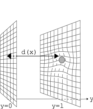
Figure 1: Radion as a distance between two branes.

We place the branes at $y=0$ ($A$-brane) and $y=l$ ($B$-brane) in this coordinate system. The proper distance between the two branes with fixed $x$ coordinates can be written as

$$d(x)=\int_{0}^{l}e^{\phi(y,x)}dy\ .$$ (5)

Hence, we call $\phi$ the radion. In this coordinate system, the 5-dimensional Einstein equations become

$$e^{-\phi}(e^{-\phi}K^{\mu}_{\ \nu})_{,y}-(e^{-\phi}K)(e^{-\phi}K^{\mu}_{\ \nu})+{\mathop{R^{\mu}_{\ \nu}}^{(4)}}-\nabla^{\mu}\nabla_{\nu}\phi-\nabla^{\mu}\phi\nabla_{\nu}\phi$$

$$\qquad=-{4\over l^{2}}\delta^{\mu}_{\nu}+\kappa^{2}\left({1\over 3}\delta^{\mu}_{\nu}\sigma_{A}+T^{A\mu}_{\quad\nu}-{1\over 3}\delta^{\mu}_{\nu}T^{A}\right)e^{-\phi}\delta(y)+\kappa^{2}\left({1\over 3}\delta^{\mu}_{\nu}\sigma_{B}+\tilde{T}^{B\mu}_{\quad\nu}-{1\over 3}\delta^{\mu}_{\nu}\tilde{T}^{B}\right)e^{-\phi}\delta(y-l)\ ,$$ (6)

$$e^{-\phi}(e^{-\phi}K)_{,y}-(e^{-\phi}K^{\alpha\beta})(e^{-\phi}K_{\alpha\beta})-\nabla^{\alpha}\nabla_{\alpha}\phi-\nabla^{\alpha}\phi\nabla_{\alpha}\phi$$

$$\qquad=-{4\over l^{2}}-{\kappa^{2}\over 3}\left(-4\sigma_{A}+T^{A}\right)e^{-\phi}\delta(y)-{\kappa^{2}\over 3}\left(-4\sigma_{B}+\tilde{T}^{B}\right)e^{-\phi}\delta(y-l)\ ,$$ (7)

$$\nabla_{\nu}(e^{-\phi}K_{\mu}^{\ \nu})-\nabla_{\mu}(e^{-\phi}K)=0\ ,$$ (8)

where $\mathop{R^{\mu}_{\ \nu}}^{(4)}$ is the curvature on the brane and $\nabla_{\mu}$ denotes the covariant derivative with respect to the metric $g_{\mu\nu}$. And we introduced the tensor $K_{\mu\nu}=-g_{\mu\nu,y}/2$ for convenience. One can read off the junction condition from the above equations as

$$e^{-\phi}\left[K^{\mu}_{\nu}-\delta^{\mu}_{\nu}K\right]|_{y=0} = {\kappa^{2}\over 2}\left(-\sigma_{A}\delta^{\mu}_{\nu}+T^{A\mu}_{\quad\nu}\right)\ ,$$ (9)

$$e^{-\phi}\left[K^{\mu}_{\nu}-\delta^{\mu}_{\nu}K\right]|_{y=l} = -{\kappa^{2}\over 2}\left(-\sigma_{B}\delta^{\mu}_{\nu}+\tilde{T}^{B\mu}_{\quad\nu}\right)\ ,$$ (10)

where $K^{\mu}_{\nu}=g^{\mu\alpha}K_{\alpha\nu}$ and the fact that we are considering a $Z_{2}$ symmetric spacetime is used. Decompose the extrinsic curvature into the traceless part and the trace part

$$e^{-\phi}K_{\mu\nu}=\Sigma_{\mu\nu}+{1\over 4}g_{\mu\nu}Q\ ,\quad Q=-e^{-\phi}{\partial\over\partial y}\log\sqrt{-g}\ .$$ (11)

Then, off the brane, we obtain the basic equations;

$$e^{-\phi}\Sigma^{\mu}_{\ \nu,y}-Q\Sigma^{\mu}_{\ \nu}=-\left[\mathop{R^{\mu}_{\ \nu}}^{(4)}-{1\over 4}\delta^{\mu}_{\nu}\mathop{R}^{(4)}-\nabla^{\mu}\nabla_{\nu}\phi-\nabla^{\mu}\phi\nabla_{\nu}\phi+{1\over 4}\delta^{\mu}_{\nu}\left(\nabla^{\alpha}\nabla_{\alpha}\phi+\nabla^{\alpha}\phi\nabla_{\alpha}\phi\right)\right]\ ,$$ (12)

$${3\over 4}Q^{2}-\Sigma^{\alpha}_{\ \beta}\Sigma^{\beta}_{\ \alpha}=\left[\mathop{R}^{(4)}\right]+{12\over l^{2}}\ ,$$ (13)

$$e^{-\phi}Q_{,y}-{1\over 4}Q^{2}-\Sigma^{\alpha\beta}\Sigma_{\alpha\beta}=\nabla^{\alpha}\nabla_{\alpha}\phi+\nabla^{\alpha}\phi\nabla_{\alpha}\phi-{4\over l^{2}}\ ,$$ (14)

$$\nabla_{\lambda}\Sigma_{\mu}^{\ \lambda}-{3\over 4}\nabla_{\mu}Q=0\ .$$ (15)

And the junction conditions are

$$\left[\Sigma^{\mu}_{\nu}-{3\over 4}\delta^{\mu}_{\nu}Q\right]\Bigg{|}_{y=0} = {\kappa^{2}\over 2}(-\sigma_{A}\delta^{\mu}_{\nu}+T^{A\mu}_{\quad\nu})\ ,$$ (16)

$$\left[\Sigma^{\mu}_{\nu}-{3\over 4}\delta^{\mu}_{\nu}Q\right]\Bigg{|}_{y=l} = -{\kappa^{2}\over 2}(-\sigma_{B}\delta^{\mu}_{\nu}+\tilde{T}^{B\mu}_{\quad\nu})\ .$$ (17)

The problem now is separated into two parts. First, we must solve the bulk equations of motion with the Dirichlet boundary condition at the A-brane, $g_{\mu\nu}(y=0,x^{\mu})=h_{\mu\nu}(x^{\mu})$. Then, the junction condition is imposed at each brane. As the junction conditions constrain the induced metrics on both branes, they naturally give rise to the effective equations of motion for the gravity on the branes.

II.2 Low Energy Expansion Scheme

Unfortunately, it is a formidable task to solve the 5-dimensional Einstein equations exactly. However, notice that typically the length scale of the internal space is $l\ll 0.1$ mm. On the other hand, usual astrophysical and cosmological phenomena take place at scales much larger than this scale. Then we need only the low energy effective theory to analyze the variety of problems, for example, the formation of a black hole, the propagation of gravitational waves, the evolution of cosmological perturbations, and so on. It should be stressed that the low energy does not necessarily implies weak gravity on the branes.

Along the normal coordinate $y$, the metric varies with the characteristic length scale $l$; $g_{\mu\nu,y}\sim g_{\mu\nu}/l$. Denote the characteristic length scale of the curvature on the brane as $L$. Then we have $R\sim g_{\mu\nu}/L^{2}$. For reader’s reference, let us take $l=1$ mm, for example. Then, the relations in the RS1 model

$$\kappa^{2}\sigma_{A}={6\over l}\ ,\qquad{\kappa^{2}\over l}=8\pi G_{N}$$ (18)

give $\kappa^{2}\sim(10^{8}{\rm GeV})^{-3}$ and $|\sigma_{i}|\sim 1{\rm TeV}^{4}$.

In this paper, we will consider the low energy regime in the sense that the energy density of the matter, $\rho_{i}$, on a brane is smaller than the brane tension, i.e., $\rho_{i}/|\sigma_{i}|\ll 1$. In this regime, a simple dimensional analysis,

$${\rho_{i}\over|\sigma_{i}|}\sim{l\over\kappa^{2}|\sigma_{i}|}\,{\kappa^{2}\rho_{i}\over l}\sim({l\over L})^{2}\ll 1$$ (19)

implies that the curvature on the brane can be neglected compared with the extrinsic curvature at low energies. Thus, the Anti-Newtonian or gradient expansion method used in the cosmological context tomita is applicable to our problem.

Our iteration scheme is to write the metric $g_{\mu\nu}$ as a sum of local tensors built out of the induced metric on the brane, with the number of derivatives increasing with the order of iteration, that is, $O((l/L)^{2n})$, $n=0,1,2,\cdots$. Hence, we seek the metric as a perturbative series

$$g_{\mu\nu}(y,x^{\mu})=a^{2}(y,x)\left[h_{\mu\nu}(x^{\mu})+g^{(1)}_{\mu\nu}(y,x^{\mu})+g^{(2)}_{\mu\nu}(y,x^{\mu})+\cdots\right]\ ,$$ (20)

$$g^{(n)}_{\mu\nu}(y=0,x^{\mu})=0\ ,\quad n=1,2,3,...$$ (21)

where the factor $a^{2}(y,x)$ is extracted because of the reason explained later and we put the Dirichlet boundary condition $g_{\mu\nu}(y=0,x)=h_{\mu\nu}(x)$ at the $A$-brane. We do not need to know the geometry of the $B$-brane when we focus on the effective equations on the $A$-brane. In other words, from the viewpoint on the $A$-brane, the junction condition at the $B$-brane simply gives the boundary condition for the bulk geometry. Other quantities are also expanded as

$$\Sigma^{\mu}_{\ \nu}=\Sigma^{(0)\mu}_{\quad\ \nu}+\Sigma^{(1)\mu}_{\quad\ \nu}+\Sigma^{(2)\mu}_{\quad\ \nu}+\cdots\ .$$ (22)

In Appendix A, we illustrate our method using a simple scalar field example to clarify the relation of the low energy expansion with the zero mode and Kaluza-Klein modes in the linearized theory.

III Background Geometry

As we can ignore the matter at the lowest order, we obtain the vacuum brane. Namely, we have an almost flat brane compared with the curvature scale of the bulk space-time. At the 0-th order, we can neglect the curvature term. Then, we have

$$e^{-\phi}\Sigma^{(0)\mu}_{\quad\ \nu,y}-Q^{(0)}\Sigma^{(0)\mu}_{\quad\ \nu}=0\ ,$$ (23)

$${3\over 4}Q^{(0)2}-\Sigma^{(0)\alpha}_{\quad\ \beta}\Sigma^{(0)\beta}_{\quad\ \alpha}={12\over l^{2}}\ ,$$ (24)

$$e^{-\phi}Q^{(0)}_{,y}-{1\over 4}Q^{(0)2}-\Sigma^{(0)\alpha\beta}\Sigma^{(0)}_{\alpha\beta}=-{4\over l^{2}}\ ,$$ (25)

$$\nabla_{\lambda}\Sigma^{(0)\ \lambda}_{\quad\ \mu}-{3\over 4}\nabla_{\mu}Q^{(0)}=0\ .$$ (26)

The junction condition is

$$\left[\Sigma^{(0)\mu}_{\quad\ \nu}-{3\over 4}\delta^{\mu}_{\nu}Q^{(0)}\right]\Bigg{|}_{y=0} = -{\kappa^{2}\over 2}\sigma_{A}\delta^{\mu}_{\nu}\ ,$$ (27)

$$\left[\Sigma^{(0)\mu}_{\quad\ \nu}-{3\over 4}\delta^{\mu}_{\nu}Q^{(0)}\right]\Bigg{|}_{y=l} = {\kappa^{2}\over 2}\sigma_{B}\delta^{\mu}_{\nu}\ .$$ (28)

Using Eq. (11), Eq. (23) can be readily integrated,

$$\Sigma^{(0)\mu}_{\quad\ \nu}={C^{\mu}_{\ \nu}(x^{\mu})\over\sqrt{-g}}\ ,\qquad C^{\mu}_{\ \mu}=0\ ,$$ (29)

where $C^{\mu}_{\ \nu}$ is a “constant” of integration. This term is not allowed to exist because of the junction conditions (27) and (28). Then, it is easy to solve the remaining equations. The result is

$$\Sigma^{(0)\mu}_{\quad\ \nu}=0\ ,\qquad Q^{(0)}={4\over l}\ .$$ (30)

Using the definition

$$K^{(0)}_{\mu\nu}=-{1\over 2}{\partial\over\partial y}g^{(0)}_{\mu\nu}=\frac{1}{l}e^{\phi}g^{(0)}_{\mu\nu}\ ,$$ (31)

we get the 0-th order metric as

$$ds^{2}=e^{2\phi(y,x)}dy^{2}+a^{2}(y,x)h_{\mu\nu}(x^{\mu})dx^{\mu}dx^{\nu}\ ,\qquad a(y,x)=\exp\left[-{1\over l}\int^{y}_{0}dye^{\phi(y,x)}\right]\ ,$$ (32)

where the tensor $h_{\mu\nu}$ is the induced metric on the positive tension brane. Note that the metric derived by Charmousis et al., $e^{\phi}=1+2f(x)e^{2y/l}/l$, is consistent with this solution CR . To proceed further, we take the coordinate system to be $\phi(y,x)=\phi(x)$. Then, we have $a(y,x)=\exp[-ye^{\phi}/l]$. Though this choice of the coordinate system is generally possible at least locally, there may be a global obstruction. However, as we show below, we can consistently get non-trivial solutions. Moreover, we explicitly demonstrate the validity of our choice at the level of linear theory in Appendix B.

Given the 0-th order solution, junction conditions (27) and (28) lead to the well known relations

$$\kappa^{2}\sigma_{A}=\frac{6}{l}\ ,\quad\kappa^{2}\sigma_{B}=-\frac{6}{l}\ .$$ (33)

Note that $\phi(x)$ and $h_{\mu\nu}(x)$ are arbitrary functions of $x$ at the 0-th order.

IV Holographic Quasi-Scalar-Tensor Gravity

IV.1 Bulk Geometry

The next order solution is obtained by taking into account the terms neglected at the 0-th order. It is at this order that the effect of matter comes in. At the 1-st order, Eqs. (12-15) become

$$e^{-\phi}\Sigma^{(1)\mu}_{\quad\ \nu,y}-{4\over l}\Sigma^{(1)\mu}_{\quad\ \nu}=-\left[\mathop{R^{\mu}_{\ \nu}}^{(4)}-\nabla^{\mu}\nabla_{\nu}\phi-\nabla^{\mu}\phi\nabla_{\nu}\phi\right]^{(1)}_{\rm traceless}\ ,$$ (34)

$${6\over l}Q^{(1)}=\left[\mathop{R}^{(4)}\right]^{(1)}\ ,$$ (35)

$$e^{-\phi}Q^{(1)}_{,y}-{2\over l}Q^{(1)}=\left[\nabla^{\alpha}\nabla_{\alpha}\phi+\nabla^{\alpha}\phi\nabla_{\alpha}\phi\right]^{(1)}\ ,$$ (36)

$$\nabla_{\lambda}\Sigma_{\quad\mu}^{(1)\ \lambda}-{3\over 4}\nabla_{\mu}Q^{(1)}=0\ ,$$ (37)

where the subscript “traceless” represents the traceless part of the quantity in the square brackets. The junction conditions are given by

$$\left[\Sigma^{(1)\mu}_{\quad\ \nu}-{3\over 4}\delta^{\mu}_{\nu}Q^{(1)}\right]\Bigg{|}_{y=0} = {\kappa^{2}\over 2}T^{A\mu}_{\quad\nu}\ ,$$ (38)

$$\left[\Sigma^{(1)\mu}_{\quad\ \nu}-{3\over 4}\delta^{\mu}_{\nu}Q^{(1)}\right]\Bigg{|}_{y=l} = -{\kappa^{2}\over 2}\tilde{T}^{B\mu}_{\quad\nu}\ ,$$ (39)

where the superscript $(1)$ represents the order of the gradient expansion. Here, $[R^{(4)\mu}_{\quad\ \nu}]^{(1)}$ means the Ricci tensor of $a^{2}h_{\mu\nu}$. Note that now $a=\exp[-ye^{\phi}/l]$. It is convenient to introduce the Ricci tensor of $h_{\mu\nu}$, denoted by $R^{\mu}_{\nu}(h)$, and express $[R^{(4)\mu}_{\quad\ \nu}]^{(1)}$ in terms of $R^{\mu}_{\nu}$ and $\phi$;

$$\left[\mathop{R^{\mu}_{\ \nu}}^{(4)}(g)\right]^{(1)}={1\over a^{2}}\left[R^{\mu}_{\ \nu}(h)+2{y\over l}e^{\phi}\left(\phi^{|\mu}_{\ |\nu}+\phi^{|\mu}\phi_{|\nu}\right)+\delta^{\mu}_{\nu}{y\over l}e^{\phi}\left(\phi^{|\alpha}_{\ |\alpha}+\phi^{|\alpha}\phi_{|\alpha}\right)+2{y^{2}\over l^{2}}e^{2\phi}\phi^{|\mu}\phi_{|\nu}-2\delta^{\mu}_{\nu}{y^{2}\over l^{2}}e^{2\phi}\phi^{|\alpha}\phi_{|\alpha}\right]\ ,$$ (40)

where $|$ denotes the covariant derivative with respect to $h_{\mu\nu}$. Similarly it is convenient to express the second derivatives of $\phi$ as

$$\left[\nabla^{\mu}\nabla_{\nu}\phi\right]^{(1)}={1\over a^{2}}\left[\phi^{|\mu}_{\ |\nu}+2{y\over l}e^{\phi}\phi^{|\mu}\phi_{|\nu}-{y\over l}e^{\phi}\delta^{\mu}_{\nu}\phi^{|\alpha}\phi_{|\alpha}\right].$$ (41)

Substituting the trace of Eq. (40) into the right-hand side of Eq. (35), we obtain

$$Q^{(1)}={l\over a^{2}}\left[{1\over 6}R(h)+{ye^{\phi}\over l}\left(\phi^{|\alpha}_{\ |\alpha}+\phi^{|\alpha}\phi_{|\alpha}\right)-{y^{2}e^{2\phi}\over l^{2}}\phi^{|\alpha}\phi_{|\alpha}\right]\ .$$ (42)

Note that Eq. (36) is trivially satisfied now. Hereafter, we omit the argument of the curvature for simplicity. Substituting Eqs. (40) and (41) into Eq. (34) and integrating it, we obtain the traceless part of the extrinsic curvature as

$$\Sigma^{(1)\mu}_{\quad\nu}={l\over a^{2}}\left[{1\over 2}\left(R^{\mu}_{\ \nu}-{1\over 4}\delta^{\mu}_{\nu}R\right)+{ye^{\phi}\over l}\left(\phi^{|\mu}_{\ |\nu}-{1\over 4}\delta^{\mu}_{\nu}\phi^{|\alpha}_{\ |\alpha}\right)+({y^{2}e^{2\phi}\over l^{2}}+{ye^{\phi}\over l})\left(\phi^{|\mu}\phi_{|\nu}-{1\over 4}\delta^{\mu}_{\nu}\phi^{|\alpha}\phi_{|\alpha}\right)\right]+{\chi^{\mu}_{\ \nu}(x)\over a^{4}}\ ,$$ (43)

where $\chi^{\mu}_{\nu}$ is an integration constant with the property $\chi^{\mu}_{\ \mu}=0$. And $\chi^{\mu}_{\nu}$ must be transverse $\chi^{\mu}_{\ \nu|\mu}=0$ in order to satisfy Eq. (37). The definition (11) gives

$$-\frac{1}{2}e^{-\phi}g^{(0)\alpha\mu}\frac{\partial}{\partial y}g^{(1)}_{\alpha\nu}=\Sigma^{(1)\mu}_{\quad\nu}+\frac{1}{4}\delta^{\mu}_{\nu}Q^{(1)}\ .$$ (44)

Integrating Eq. (44), we obtain the metric in the bulk:

$$g^{(1)}_{\mu\nu} = -{l^{2}\over 2}\left({1\over a^{2}}-1\right)(R_{\mu\nu}-{1\over 6}h_{\mu\nu}R)+{l^{2}\over 2}\left({1\over a^{2}}-1-{2ye^{\phi}\over l}{1\over a^{2}}\right)\left(\phi_{|\mu\nu}+{1\over 2}h_{\mu\nu}\phi^{|\alpha}\phi_{|\alpha}\right)$$ (45)

$$\quad-{y^{2}e^{2\phi}\over a^{2}}\left(\phi_{|\mu}\phi_{|\nu}-{1\over 2}h_{\mu\nu}\phi^{|\alpha}\phi_{|\alpha}\right)-{l\over 2}\left({1\over a^{4}}-1\right)\chi_{\mu\nu}\ ,$$

where we have imposed the boundary condition, $g^{(1)}_{\mu\nu}(y=0,x^{\mu})=0$. From these results, one can calculate the Weyl tensor as

$$C_{y\mu y\nu}={2\chi_{\mu\nu}\over la^{4}}\ .$$ (46)

Hence, the term of $\chi_{\mu\nu}$ is essentially the Weyl tensor at this order. Note that we have obtained the bulk metric in terms of $\phi(x)$, $h_{\mu\nu}(x)$ and $\chi_{\mu\nu}(x)$.

IV.2 Quasi-Scalar-Tensor Gravity

We shall deduce the equations for $\phi(x),\ h_{\mu\nu}(x)$ and $\chi_{\mu\nu}(x)$ from junction conditions. Using Eqs. (42) and (43), one gets the junction conditions. The junction condition at the $A$-brane is written as

$${l\over 2}G^{\mu}_{\ \nu}(h)+\chi^{\mu}_{\ \nu}={\kappa^{2}\over 2}T^{A\mu}_{\quad\ \nu}\ .$$ (47)

This equation is nothing but the Einstein equations with the generalized dark radiation $\chi_{\mu\nu}$. It should be noted that $\chi_{\mu\nu}$ is undetermined at this level, exhibiting the non-local nature of Eq. (47).

The junction condition at the $B$-brane is given by

$${l\over 2\Omega^{2}}G^{\mu}_{\ \nu}+{le^{\phi}\over\Omega^{2}}\left(\phi^{|\mu}_{\ |\nu}-\delta^{\mu}_{\nu}\phi^{|\alpha}_{\ |\alpha}+\phi^{|\mu}\phi_{|\nu}-\delta^{\mu}_{\nu}\phi^{|\alpha}\phi_{|\alpha}\right)+{le^{2\phi}\over\Omega^{2}}\left(\phi^{|\mu}\phi_{|\nu}+{1\over 2}\delta^{\mu}_{\nu}\phi^{|\alpha}\phi_{|\alpha}\right)+{\chi^{\mu}_{\ \nu}\over\Omega^{4}}=-{\kappa^{2}\over 2\Omega^{2}}T^{B\mu}_{\quad\nu}\ ,$$ (48)

where $\Omega(x)=a(y=l,x)=\exp[-e^{\phi}]$. Here, the index of $T^{B\mu}_{\quad\ \nu}$ is the energy momentum tensor with the index raised by the induced metric $h_{\mu\nu}$ on the $A$-brane, while $\tilde{T}^{B\mu}_{\quad\ \nu}$ is the one raised by the induced metric on the $B$-brane. At the present order, we have the following relations,

$$T^{B}_{\mu\nu}=\tilde{T}^{B}_{\mu\nu}\ ,\ T^{B\mu}_{\quad\nu}=\Omega^{2}\tilde{T}^{B\mu}_{\quad\nu}\ .$$ (49)

To reveal the role of the radion field, we must write Eq. (48) using the induced metric on the $B$-brane $g^{B{\rm brane}}_{\mu\nu}=\Omega^{2}(h_{\mu\nu}+g^{(1)}_{\mu\nu})\equiv f_{\mu\nu}+\Omega^{2}g^{(1)}_{\mu\nu}$. At this order, the Ricci tensor $R^{\mu}_{\nu}$ of the induced metric on the $B$-brane is equal to that of $f_{\mu\nu}$. Using this fact, we rewrite Eq. (48) to obtain the effective equations on the $B$-brane,

$${l\over 2}G^{\mu}_{\ \nu}(f)+{\chi^{\mu}_{\ \nu}\over\Omega^{4}}=-{\kappa^{2}\over 2}\tilde{T}^{B\mu}_{\quad\nu}\ .$$ (50)

Again, we have the non-conventional (non-local) Einstein equations as in the case of the $A$-brane.

Although Eqs. (47) and (50) are non-local individually, with undetermined $\chi_{\mu\nu}$, one can combine both equations to reduce them to local equations for each brane. This happens to be possible since $\chi_{\mu\nu}$ appears only algebraically; one can easily eliminate $\chi_{\mu\nu}$ from Eqs. (47) and (48). Defining a new field $\Psi=1-\Omega^{2}$, we find

$$G^{\mu}_{\ \nu}(h)={\kappa^{2}\over l\Psi}T^{A\mu}_{\quad\ \nu}+{\kappa^{2}(1-\Psi)\over l\Psi}T^{B\mu}_{\quad\ \nu}+{1\over\Psi}\left(\Psi^{|\mu}_{\ |\nu}-\delta^{\mu}_{\nu}\Psi^{|\alpha}_{\ |\alpha}\right)+{\omega(\Psi)\over\Psi^{2}}\left(\Psi^{|\mu}\Psi_{|\nu}-{1\over 2}\delta^{\mu}_{\nu}\Psi^{|\alpha}\Psi_{|\alpha}\right)\ ,$$ (51)

where the coupling function $\omega(\Psi)$ takes the following form:

$$\omega(\Psi)={3\over 2}{\Psi\over 1-\Psi}\ .$$ (52)

We can also determine $\chi^{\mu}_{\nu}$ by eliminating $G^{\mu}_{\nu}$ from Eqs. (47) and (48). Then,

$$\chi^{\mu}_{\ \nu}=-{\kappa^{2}(1-\Psi)\over 2\Psi}\left(T^{A\mu}_{\quad\nu}+T^{B\mu}_{\quad\nu}\right)-{l\over 2\Psi}\left[\left(\Psi^{|\mu}_{\ |\nu}-\delta^{\mu}_{\nu}\Psi^{|\alpha}_{\ |\alpha}\right)+{\omega(\Psi)\over\Psi}\left(\Psi^{|\mu}\Psi_{|\nu}-{1\over 2}\delta^{\mu}_{\nu}\Psi^{|\alpha}\Psi_{|\alpha}\right)\right]\ .$$ (53)

The condition $\chi^{\mu}_{\ \mu}=0$ gives rise to the field equation for $\Psi$:

$$\Box\Psi={\kappa^{2}\over l}{T^{A}+T^{B}\over 2\omega+3}-{1\over 2\omega+3}{d\omega\over d\Psi}\Psi^{|\mu}\Psi_{|\mu}\ ,$$ (54)

where we have used the explicit form of $\omega(\Psi)$. This equation tells us that the trace part of the energy momentum tensor determines the radion field and hence the relative bending of the brane. And $\chi_{\mu\nu}$ is determined by the traceless part of the right-hand side of Eq. (53). Remarkably, $\chi_{\mu\nu}$ is now a secondary entity.

Eqs. (51) and (54) are the basic equations to be used in cosmological or astrophysical contexts when the characteristic energy density is less than $|\sigma_{i}|$. Notice that the conservation law with respect to the metric $h_{\mu\nu}$ reads

$$T^{A\mu}_{\quad\ \nu|\mu}=0\ ,\quad T^{B\mu}_{\quad\ \nu|\mu}={\Psi_{|\mu}\over 1-\Psi}T^{B\mu}_{\quad\ \nu}-{1\over 2}{\Psi_{|\nu}\over 1-\Psi}T^{B}\ .$$ (55)

In contrast to the usual scalar-tensor gravity, this theory couples with two kinds of matter, namely, the matters on both positive and negative tension branes, with different effective gravitational coupling constants. For this reason, we call this theory the quasi-scalar-tensor gravity. Thus, the (non-local) Einstein equations (47) with the generalized dark radiation has transformed into the (local) quasi-scalar-tensor gravity (51) with the coupling function $\omega(\Psi)$.

IV.3 Effective Action

Let us consider an effective action for $h_{\mu\nu}(x)$ and $\phi(x)$. If one wants to calculate the quantum fluctuations in the inflationary scenario, for example, one needs the action to determine the magnitudes of them. The action have to be derived from the original 5-dimensional action by substituting the solution of the equations of motion in the bulk and integrating out over the bulk coordinate. We shall start with the following action:

$$S = {1\over 2\kappa^{2}}\int d^{5}x\sqrt{-g}\left[{\cal R}+{12\over l^{2}}\right]+{2\over\kappa^{2}}\int d^{4}x\sqrt{-h}Q^{A}-{2\over\kappa^{2}}\int d^{4}x\sqrt{-f}Q^{B}$$ (56)

$$-{6\over\kappa^{2}l}\int d^{4}x\sqrt{-h}+{6\over\kappa^{2}l}\int d^{4}x\sqrt{-f}+\int d^{4}x\sqrt{-h}{\cal L}^{A}+\int d^{4}x\sqrt{-f}{\cal L}^{B}\ ,$$

where we have taken into account the boundary term, the so-called Gibbons-Hawking term instead of introducing delta-function singularities in the curvature. The factor 2 in the Gibbons-Hawking term comes from the $Z_{2}$ symmetry of this space-time. As we substitute the solution of the bulk equations of motion, we can use the the equation ${\cal R}=-20/l^{2}$ which holds in the bulk. It should be stressed that the bulk metric is solved without using junction conditions and is expressed in terms of $\phi$, $h_{\mu\nu}$ and $\chi_{\mu\nu}$. That is why we can get the effective action on the brane by the simple substitution of the solution. Now, up to the first order, we obtain

$$S = -{8\over\kappa^{2}l^{2}}\int d^{4}x\sqrt{-h}\int_{0}^{le^{\phi}}dza^{4}\left[1+{1\over 2}h^{\mu\nu}g^{(1)}_{\mu\nu}\right]+{2\over\kappa^{2}}\int d^{4}x\sqrt{-h}\left[{4\over l}+{l\over 6}R\right]$$ (57)

$$\quad-{2\over\kappa^{2}}\int d^{4}x\sqrt{-h}\Omega^{4}\left[1+{1\over 2}h^{\mu\nu}g^{(1)}_{\mu\nu}\right]\left[{4\over l}+{l\over 6\Omega^{2}}R+{le^{\phi}\over\Omega^{2}}\left(\Box\phi+\phi^{|\alpha}\phi_{|\alpha}\right)-{le^{2\phi}\over\Omega^{2}}\phi^{|\alpha}\phi_{|\alpha}\right]$$

$$\quad-{6\over\kappa^{2}l}\int d^{4}x\sqrt{-h}+{6\over\kappa^{2}l}\int d^{4}x\sqrt{-h}\Omega^{4}\left[1+{1\over 2}h^{\mu\nu}g^{(1)}_{\mu\nu}\right]+\int d^{4}x\sqrt{-h}{\cal L}^{A}+\int d^{4}x\sqrt{-h}\Omega^{4}{\cal L}^{B}\ .$$

Using Eq. (45) and the definition $\Psi=1-\Omega^{2}$, we finally have the action:

$$S={l\over 2\kappa^{2}}\int d^{4}x\sqrt{-h}\left[\Psi R-{\omega(\Psi)\over\Psi}\Psi^{|\alpha}\Psi_{|\alpha}\right]+\int d^{4}x\sqrt{-h}{\cal L}^{A}+\int d^{4}x\sqrt{-h}\left(1-\Psi\right)^{2}{\cal L}^{B}\ .$$ (58)

This is a complete derivation of the action with the correct normalization which is important for quantization of the theory.

Here, it should be noted that $\chi^{\mu}_{\nu}$ which appeared in $g^{(1)}_{\mu\nu}$ is a non-local quantity. In fact, eliminating $\Psi$ from Eq. (53) by solving Eq. (54) yields a non-local expression of $\chi^{\mu}_{\nu}$. If we substitute this non-local expression into Eq. (47), we will obtain a non-local theory. Conversely, one can see that introducing the radion disentangles the non-locality in the non-conventional Einstein equations (47) and yields the quasi-scalar-tensor gravity given by Eqs. (51) and (54). This important point is more transparent in the derivation of the effective action. Indeed, the non-local part $\chi^{\mu}_{\nu}$ disappears because of the traceless nature $\chi^{\mu}_{\mu}=0$. A similar mechanism is discussed by Gen and Sasaki gen in the context of the linear theory.

IV.4 Holographic Brane Gravity

We have obtained the 4-dimensional quasi-scalar-tensor gravity from the 5-dimensional action. The bulk metric corresponding to the 4-dimensional effective theory is given by

$$g_{\mu\nu}=(1-\Psi)^{y/l}\left[h_{\mu\nu}(x)+g^{(1)}_{\mu\nu}(h_{\mu\nu},\Psi,T^{A}_{\mu\nu},T^{B}_{\mu\nu},y)\right]\ ,$$ (59)

where $\chi_{\mu\nu}$ in Eq. (45) is eliminated by using Eq. (53). Here, the $y$-dependence of $g^{(1)}_{\mu\nu}$ is explicitly known. Thus the bulk metric is completely determined by the energy momentum tensors on both branes and the radion and the induced metric on the $A$-brane. Therefore, once the 4-dimensional solution of the quasi-scalar-tensor gravity is given, one can reconstruct the bulk geometry from these data. The quasi-scalar-tensor gravity works as holograms at the low energy. In this sense, one can call the quasi-scalar-tensor gravity the holographic brane gravity. Eq. (59) gives a holographic picture of the brane world. Recalling that the radion specifies the position of the second brane, the radion can be interpreted as a kind of “phase” in the holographic picture of the brane world.

IV.5 Effective Theory on $B$-brane

For completeness, we shall derive the effective equations of motion on the $B$-brane. To do so, let us simply reverse the role of the $A$-brane and that of the $B$-brane. Substituting $h_{\mu\nu}=\Omega^{-2}f_{\mu\nu}$ into the junction conditions yields

$${l\over 2}G^{\mu}_{\ \nu}(f)+{\chi^{\mu}_{\ \nu}\over\Omega^{4}}=-{\kappa^{2}\over 2}T^{B\mu}_{\ \nu}$$ (60)

and

$${l\Omega^{2}\over 2}G^{\mu}_{\ \nu}+l\Omega^{2}\left((\log\Omega)^{;\mu}_{\ ;\nu}-\delta^{\mu}_{\nu}(\log\Omega)^{;\alpha}_{;\alpha}+(\log\Omega)^{;\mu}(\log\Omega)_{;\nu}+{1\over 2}\delta^{\mu}_{\nu}(\log\Omega)^{;\alpha}(\log\Omega)_{;\alpha}\right)+\chi^{\mu}_{\ \nu}={\kappa^{2}\Omega^{2}\over 2}T^{A\mu}_{\ \nu}\ ,$$ (61)

where ; denotes the covariant derivative with respect to the metric $f_{\mu\nu}$. Thus, defining $\Phi=\Omega^{-2}-1$, we obtain the effective equation on the $B$-brane:

$$G^{\mu}_{\ \nu}(f)={\kappa^{2}\over l\Phi}T^{B\mu}_{\quad\ \nu}+{\kappa^{2}(1+\Phi)\over l\Phi}T^{A\mu}_{\quad\ \nu}+{1\over\Phi}\left(\Phi^{;\mu}_{\ ;\nu}-\delta^{\mu}_{\nu}\Phi^{;\alpha}_{\ ;\alpha}\right)+{\omega(\Phi)\over\Phi^{2}}\left(\Phi^{;\mu}\Phi_{;\nu}-{1\over 2}\delta^{\mu}_{\nu}\Phi^{;\alpha}\Phi_{;\alpha}\right)\ ,$$ (62)

where

$$\omega(\Phi)=-{3\over 2}{\Phi\over 1+\Phi}\ .$$ (63)

The equations of motion for the radion becomes

$$\Box\Phi={\kappa^{2}\over l}{T^{A}+T^{B}\over 2\omega+3}-{1\over 2\omega+3}{d\omega\over d\Phi}\Phi^{;\mu}\Phi_{;\mu}\ .$$ (64)

Thus, we have shown that the gravity on the negative tension brane is described by the quasi-scalar-tensor gravity with a coupling function $\omega(\Phi)=-3\Phi/2(1+\Phi)$.

It should be noted that the dynamics on both branes are not independent. We know the gravity on the $B$-brane once we know that on the $A$-brane, and vice versa. The transformation rules are

$$\Phi = {\Psi\over 1-\Psi}\ ,$$ (65)

$$g^{B{\rm brane}}_{\mu\nu} = (1-\Psi)\left[h_{\mu\nu}+g^{(1)}_{\mu\nu}\left(h_{\mu\nu},\Psi,T^{A}_{\mu\nu},T^{B}_{\mu\nu},\ y=l\right)\right]\ .$$ (66)

This relation is useful when we consider concrete applications.

V Kaluza-Klein corrections

As explained in Appendix A, our analysis so far to the first order in the gradient expansion corresponds to the zero-mode truncation in the language of the linearized theory. Although it is obscure to use the word “Kaluza-Klein corrections” in the non-linear theory, we shall call their non-linear counterpart simply as Kaluza-Klein corrections in this paper.

In principle, we can continue our analysis up to a desired order using the following recursive formulas:

$$\Sigma^{(n)\mu}_{\quad\ \nu}=-{1\over a^{4}}\int dya^{4}\left\{\left[\mathop{R^{\mu}_{\ \nu}}^{(4)}-\nabla^{\mu}\nabla_{\nu}\phi-\nabla^{\mu}\phi\nabla_{\nu}\phi\right]^{(n)}_{\rm traceless\ part}-\sum_{p=1}^{n-1}Q^{(p)}\Sigma^{(n-p)\mu}_{\quad\quad\nu}\right\}\ ,$$ (67)

$$Q^{(n)}={l\over 6}\sum_{p=1}^{n-1}\left[-{3\over 4}Q^{(p)}Q^{(n-p)}+\Sigma^{(p)\alpha}_{\quad\ \beta}\Sigma^{(n-p)\beta}_{\quad\quad\alpha}+[\mathop{R}^{(4)}]^{(n)}\right],$$ (68)

$$Q^{(n)}_{,y}-{2\over l}Q^{(n)}=\sum_{p=1}^{n-1}\left\{{1\over 4}Q^{(p)}Q^{(n-p)}+\Sigma^{(p)\alpha\beta}\Sigma^{(n-p)}_{\alpha\beta}\right\}+\left[\nabla^{\alpha}\nabla_{\alpha}\phi+\nabla^{\alpha}\phi\nabla_{\alpha}\phi\right]^{(n)}\ ,$$ (69)

$$\Sigma_{\mu\quad\ |\lambda}^{(n)\ \lambda}-{3\over 4}Q^{(n)}_{|\mu}+\sum_{p=1}^{n-1}\left\{\Gamma^{(p)\alpha}_{\lambda\alpha}\Sigma^{(n-p)\lambda}_{\quad\quad\mu}-\Gamma^{(p)\lambda}_{\alpha\mu}\Sigma^{(n-p)\alpha}_{\quad\quad\lambda}\right\}=0\ .$$ (70)

These equations give a solution as an infinite sum. The existence of the infinite series is a manifestation of the non-locality of the brane model mukoh .

To get the effective equations of motion with second order corrections using the above formula is straightforward. However, carrying out the calculation is laborious and the resultant expression is too long to write down. As for the linear theory, we will obtain the explicit effective equations of motion with Kaluza-Klein corrections in Appendix B. Here, we will only sketch how the Kaluza-Klein corrections appear using an easy method.

Although we need the explicit $y$-dependence of the bulk to obtain the action, as long as we are interested only in the effective equations on the brane, we do not have to solve the bulk explicitly. The reason is as follows. We can write down the non-local Einstein equations corresponding to Eqs. (47) and (50) without knowing the bulk geometry. Then since we know how the non-local term, i.e., the generalized dark radiation term behaves in the bulk, we may eliminate it just as in the 1-st order case.

The non-local Einstein equations on the branes are kanno

$$G^{(4)}_{\mu\nu}(h) = -{2\over l}\left(\chi_{\mu\nu}+t_{\mu\nu}\right)+{\kappa^{2}\over l}T^{A}_{\mu\nu}-{l^{2}\over 2}{\cal S}_{\mu\nu}-{l^{2}\over 12}\left(RR_{\mu\nu}-{1\over 2}h_{\mu\nu}R^{2}+{3\over 4}h_{\mu\nu}R^{\alpha}_{\beta}R^{\beta}_{\alpha}\right)$$ (71)

$$+{l\over 2}\left[\chi^{\alpha}_{\ \mu|\nu\alpha}+\chi^{\alpha}_{\ \nu|\mu\alpha}-\chi_{\mu\nu|\alpha}^{\quad|\alpha}\right]-l\chi_{\mu\alpha}R^{\alpha}_{\ \nu}+{l\over 6}R\chi_{\mu\nu}-{1\over 4}h_{\mu\nu}\chi^{\alpha}_{\beta}\chi^{\beta}_{\alpha}$$

$$G^{(4)}_{\mu\nu}(g^{B{\rm brane}}) = -{2\over l\Omega^{4}}\left(\chi_{\mu\nu}+t_{\mu\nu}\right)-{\kappa^{2}\over l}T^{B}_{\mu\nu}-l^{2}\left(1+{\Omega^{2}\over 2}\right){\cal S}_{\mu\nu}-{l^{2}\over 12}\Omega^{2}\left(RR_{\mu\nu}-{3\over 2}g^{B{\rm brane}}_{\mu\nu}R^{\alpha}_{\beta}R^{\beta}_{\alpha}\right)$$ (72)

$$+{l\over 4}\left(1+{1\over\Omega^{4}}\right)\left[\chi^{\alpha}_{\ \mu;\nu\alpha}+\chi^{\alpha}_{\ \nu;\mu\alpha}-\chi_{\mu\nu;\alpha}^{\quad;\alpha}\right]-{l\over 2}\left(1+{1\over\Omega^{4}}\right)\left(\chi_{\mu\alpha}R^{\alpha}_{\ \nu}-{1\over 4}g^{B{\rm brane}}_{\mu\nu}\chi_{\alpha\beta}R^{\alpha\beta}\right)+{l\over 6\Omega^{4}}R\chi_{\mu\nu}$$

$$-{3\over 4}g^{B{\rm brane}}_{\mu\nu}\left[{l^{2}\over 4}\left(R^{\alpha}_{\beta}R^{\beta}_{\alpha}-{2\over 9}R^{2}\right)+{l\over 2\Omega^{4}}\chi^{\alpha}_{\beta}R^{\beta}_{\alpha}-{l\over 6}\chi^{\alpha}_{\beta}R^{\beta}_{\alpha}+{1\over 3\Omega^{8}}\chi^{\alpha}_{\beta}\chi^{\beta}_{\alpha}\right]\ .$$

where $t_{\mu\nu}$ is an integration constant at the 2-nd order and we have defined the quantity

$${\cal S}^{\mu}_{\ \nu} = R^{\mu}_{\ \alpha}R^{\alpha}_{\ \nu}-{1\over 3}RR^{\mu}_{\ \nu}-{1\over 4}\delta^{\mu}_{\nu}(R^{\alpha}_{\ \beta}R^{\beta}_{\ \alpha}-{1\over 3}R^{2})$$ (73)

$$\qquad-{1\over 2}\left(R^{\alpha\mu}_{\ \ |\nu\alpha}+R^{\alpha\ |\mu}_{\ \nu\ \ |\alpha}-{2\over 3}R^{|\mu}_{\ |\nu}-\Box R^{\mu}_{\ \nu}+{1\over 6}\delta^{\mu}_{\nu}\Box R\right)\ .$$

Here, ; represents the covariant derivative with respect to $f_{\mu\nu}$ and all of the curvatures in Eq. (71) are calculated from $g^{B{\rm brane}}_{\mu\nu}$. What we should do is to eliminate $t_{\mu\nu}$ from Eqs. (71) and (72) and substitute the relation $g^{B{\rm brane}}_{\mu\nu}=\Omega^{2}[h_{\mu\nu}+g^{(1)}_{\mu\nu}]$ into the resulting equation. Then we obtain a higher derivative but local theory on the brane.

Noticeably, the same is true for all higher order corrections. Thus, one can infer that the radion disentangles the non-locality in the system to all orders at the expense of introducing higher derivative terms.

VI Conclusion

We have developed a method to deduce the low energy effective theory for the two-brane system. The 5-dimensional equations of motion in the bulk is solved using a low energy expansion method. This allows us, through the junction conditions, to deduce the effective equations of motion for the gravity on the brane. As a result, we have shown that the gravity on the brane world is described by a quasi-scalar-tensor theory with a specific coupling function $\omega(\Psi)=3\Psi/2(1-\Psi)$ on the positive tension brane and $\omega(\Phi)=-3\Phi/2(1+\Phi)$ on the negative tension brane, where $\Psi$ and $\Phi$ are Brans-Dicke-like scalars on the positive and negative tension branes, respectively. In contrast to the usual scalar-tensor theory, the quasi-scalar-tensor theory couples with matters on both branes but with different effective gravitational coupling constants. In particular, the radion disguised as the scalar fields $\Psi$ and $\Phi$ couples with the sum of the traces of the energy momentum tensor on both branes. Moreover, we have derived the effective action by substituting the solution of the bulk equations of motion into the original action. This direct method determines the normalization of the effective action which is indispensable for quantizing the theory.

In the process of derivation of the effective equations of motion, we have clarified how the quasi-scalar tensor gravity emerges from Einstein’s theory with the generalized dark radiation term described by $\chi_{\mu\nu}$. A brane can feel the non-local effect of the bulk geometry only through $\chi_{\mu\nu}$ irrespective of the existence of another brane. This is the picture that the Einstein equations with the generalized dark radiation tells us. Then, what is the role of the radion? In order to make the connection between the radion and $\chi_{\mu\nu}$, we have to know the bulk geometry. In the case of a single brane, $\chi_{\mu\nu}$ is determined by the boundary conditions at the Cauchy horizon. If we require that the geometry is asymptotically Anti-deSitter there, then $\chi_{\mu\nu}$ must vanish wiseman2 . In the two-brane case, we have no asymptotic region, instead we have the second brane in the bulk. The radion determines the location of the second brane where the junction conditions are imposed. The junction conditions give $\chi_{\mu\nu}$ as a function of the energy momentum tensor and the radion. The resultant equation is nothing but the holographic quasi-scalar-tensor gravity. Thus, the difference between the Einstein equations with the generalized dark radiation and the quasi-scalar-tensor gravity is just superficial. The radion has converted the non-local non-conventional Einstein equations to the local quasi-scalar-tensor gravity.

We have also given a systematic method to calculate the corrections due to Kaluza-Klein massive modes. It is conjectured that all of the non-locality arising from the integration is disentangled by the radion in the two brane system. We have also emphasized the holographic aspect of our result. It turns out that the effect of the bulk gravity on the low energy physics in the brane world can be described solely in the 4-dimensional language. Conversely, the bulk geometry can be reconstructed from the knowledge of the 4-dimensional data. In this sense, the quasi-scalar-tensor gravity we have found in this paper works as holograms and hence can be called the holographic brane gravity.

Let us discuss an implication of our results. Cosmology is usually formulated on the basis of local field theory. However, the superstring theory suggests non-local field theories are ubiquitous. Though a non-local field theory is not easy to treat properly, the holographic description opens a new possibility to study cosmology with non-local terms. The brane world cosmology can be regarded as a realization of a non-local field theoretic approach to cosmology. In the single brane picture, the non-local terms due to the integration constant appear kanno . Furthermore, there are infinite series of higher derivative terms in the low energy expansion scheme. This is also a manifestation of the non-locality of the brane world gravity kanno ; mukoh . In the two brane system, there also exist the above two types of non-locality. Intriguingly, the radion has disentangled the non-locality of the homogeneous solutions and led to the quasi-scalar-tensor gravity. Hence, the quasi-scalar tensor theory is a non-local theory disguised as a local theory. In fact, integrating out the scalar field yields a non-local field theory. In addition, the non-locality due to the Kaluza-Klein type corrections remains as an infinite series in the low energy expansion even in the two brane system. Cosmology with non-local fields from this point of view deserves further investigation.

As we have succeeded to obtain the effective action for the non-linear brane gravity, various problems can be now investigated. The two brane inflation is under investigation using our method sugumi . Astrophysical applications such as gravitational waves from binary stars are also intriguing. Extension of our formalism to more general models which include bulk scalars or vector fields might be interesting.

Appendix A Scalar field Example

In order to illustrate the method used in the main text, we examine a toy model in this appendix. Let us consider a massless scalar field $\phi$ in the background

$$ds^{2}=dy^{2}+\exp[-2{y\over l}]\eta_{\mu\nu}dx^{\mu}dx^{\nu}\ ,$$ (74)

where the branes are located at $y=0$ and $y=d$. The equation of motion for $\phi$ with a source on the branes becomes

$$\Box^{(5)}\phi=e^{4y/l}\partial_{y}\left[e^{-4y/l}\partial_{y}\phi\right]+e^{2y/l}\Box\phi=J^{A}(x)\delta(y)+J^{B}(x)\delta(y-d)\ .$$ (75)

From this equation, one can deduce the junction conditions

$$\partial_{y}\phi|_{y=0} = {1\over 2}J^{A}(x)\ ,$$ (76)

$$\partial_{y}\phi|_{y=d} = -{1\over 2}J^{B}(x)\ .$$ (77)

Let us focus on the $A$-brane at $y=0$ and put

$$\phi(y=0,x)=\phi_{0}(x)\ .$$ (78)

The Green function with the Neumann boundary condition is easily calculated as

$$\Delta_{5}(0,x;0,x^{\prime}) = \int{d^{4}p\over(2\pi)^{4}}\exp[ip\cdot(x-x^{\prime})]{1\over q}{J_{1}(qle^{d/l})H^{(1)}_{2}(ql)-J_{2}(ql)H^{(1)}_{1}(qle^{d/l})\over J_{1}(qle^{d/l})H^{(1)}_{1}(ql)-J_{1}(ql)H^{(1)}_{1}(qle^{d/l})}$$ (79)

$$= \int{d^{4}p\over(2\pi)^{4}}\exp[ip\cdot(x-x^{\prime})]{2\over q^{2}l(1-e^{-2d/l})}\left[1+q^{2}l^{2}\left({3\over 8}-{1\over 8}e^{-2d/l}-{1\over 2(1-e^{-2d/l})}{d\over l}\right)+\cdots\right]\ ,$$

and

$$\Delta_{5}(0,x;d,x^{\prime}) = -{2ie^{d/l}\over\pi l}\int{d^{4}p\over(2\pi)^{4}}\exp[ip\cdot(x-x^{\prime})]{1\over q^{2}}{1\over J_{1}(qle^{d/l})H^{(1)}_{1}(ql)-J_{1}(ql)H^{(1)}_{1}(qle^{d/l})}$$ (80)

$$= \int{d^{4}p\over(2\pi)^{4}}\exp[ip\cdot(x-x^{\prime})]{2\over q^{2}l(1-e^{-2d/l})}\left[1+q^{2}l^{2}\left({1\over 8}+{1\over 8}e^{2d/l}-{1\over 2(1-e^{-2d/l})}{d\over l}\right)+\cdots\right]\ ,$$

where $q^{2}=-\eta_{\mu\nu}p^{\mu}p^{\nu}$. Thus, the standard Green function method gives the solution for Eq. (75) as

$$\phi_{0}(x)={1\over 2}\int d^{4}x^{\prime}\Delta_{5}(0,x;0,x^{\prime})J^{A}(x^{\prime})+{1\over 2}\int d^{4}x^{\prime}e^{-4d/l}\Delta_{5}(0,x;d,x^{\prime})J^{B}(x^{\prime})\ .$$ (81)

This gives

$$\Box\phi_{0}(x) = {1\over 2}\int d^{4}x^{\prime}\Box\Delta_{5}(0,x;0,x^{\prime})J^{A}(x^{\prime})+{1\over 2}\int d^{4}x^{\prime}e^{-4d/l}\Box\Delta_{5}(0,x;d,x^{\prime})J^{B}(x^{\prime})$$ (82)

$$= {1\over l(1-e^{-2d/l})}J^{A}(x)+{e^{-4d/l}\over l(1-e^{-2d/l})}e^{-4d/l}J^{B}(x)$$

$$\quad+{1\over l(1-e^{-2d/l})}\left[{3\over 8}-{1\over 8}e^{-2d/l}-{1\over 2(1-e^{-2d/l})}{d\over l}\right]l^{2}\Box J^{A}(x)$$

$$\quad+{e^{-4d/l}\over l(1-e^{-2d/l})}e^{-4d/l}\left[{1\over 8}+{1\over 8}e^{2d/l}-{1\over 2(1-e^{-2d/l})}{d\over l}\right]l^{2}\Box J^{B}(x)+\cdots\ .$$

Note that the first two terms come from the zero mode and the rest are Kaluza-Klein corrections. Now, we shall compare the above result, Eq. (82), with our method.

A.1 0-th order

At the 0-th order, we ignore gradients on the brane, then we get

$$e^{4y/l}\partial_{y}\left[e^{-4y/l}\partial_{y}\phi^{(0)}\right]=0\ .$$ (83)

The solution of Eq. (83) is given by

$$\phi^{(0)}=\phi_{0}+e^{4y/l}\psi_{0}\ .$$ (84)

However, as we are regarding the source terms as the first order quantities, the junction conditions (76) and (77) imply $\psi_{0}=0$. Hence, we simply obtain $\phi^{(0)}=\phi_{0}$.

A.2 1-st order

At the first order, we must solve

$$e^{4y/l}\partial_{y}\left[e^{-4y/l}\partial_{y}\phi^{(1)}\right]=-e^{2y/l}\Box\phi_{0}(x)\ .$$ (85)

The result is

$$\phi^{(1)}={l^{2}\over 4}e^{2y/l}\Box\phi_{0}+{l\over 4}e^{4y/l}C(x)+D(x)$$ (86)

where $C$ and $D$ are homogeneous solutions. The junction conditions (76) and (77) become

$$\partial_{y}\phi|_{y=0} = {l\over 2}\Box\phi_{0}+C={1\over 2}J^{A}(x)\ ,$$ (87)

$$\partial_{y}\phi|_{y=d} = {l\over 2}e^{2d/l}\Box\phi_{0}+Ce^{4d/l}=-{1\over 2}J^{B}(x)\ .$$ (88)

Eliminating $C$ from these equations, we obtain

$$\Box\phi_{0}={1\over l(1-e^{-2d/l})}J^{A}+{e^{-4d/l}\over l(1-e^{-2d/l})}J^{B}\ .$$ (89)

This agrees with the zero-mode part of Eq. (82). Thus our method to the first order corresponds to the zero-mode truncation when linearized. The homogeneous part is also determined as

$$C(x)={1\over 2(1-e^{2d/l})}\left[J^{A}+e^{-2d/l}J^{B}\right]\ .$$ (90)

A.3 2-nd order

At the 2-nd order, we have

$$e^{4y/l}\partial_{y}\left[e^{-4y/l}\partial_{y}\phi^{(2)}\right]=-e^{2y/l}\Box\phi^{(1)}(x)\ .$$ (91)

This Eq. (91) can be integrated as

$$\partial_{y}\phi^{(2)}=-{l^{2}\over 4}\left(ye^{4y/l}+{l\over 2}e^{2y/l}\right)\Box^{2}\phi_{0}-{l^{2}\over 8}(e^{6y/l}+e^{2y/l})\Box C(x)+e^{4y/l}D(x)\ .$$ (92)

Hence, the junction conditions (76) and (77) yield

$${l\over 2}\Box\phi_{0}+C(x)-{l^{3}\over 8}\Box^{2}\phi_{0}-{l^{2}\over 4}\Box C(x)+D(x)={1\over 2}J^{A}(x)\ ,$$ (93)

$${l\over 2}e^{2y/l}\Box\phi_{0}+C(x)e^{4y/l}-{l^{2}\over 4}(de^{4y/l}+{l\over 2}e^{2y/l})\Box^{2}\phi_{0}-{l^{2}\over 8}(e^{6y/l}+e^{2y/l})\Box C(x)+e^{4y/l}D(x)=-{1\over 2}J^{B}(x)\ .$$ (94)

Combining both Eqs. (93) and (94), we get

$$\Box\phi_{0}={1\over l(1-e^{-2d/l})}\left[J^{A}+e^{-4d/l}J^{B}\right]+\left[{l^{2}\over 4}-{ld\over 2}{1\over(1-e^{-2d/l})}\right]\Box^{2}\phi_{0}-{l\over 4}e^{2d/l}\left[1-e^{-2d/l}\right]\Box C\ .$$ (95)

Substituting Eqs. (89) and (90) into the right-hand side of Eq. (95) yields Eq. (82). Thus, we have shown that the 2-nd order equations in our method correspond to taking into account the Kaluza-Klein corrections when the equations are linearized.

Appendix B Linearized Gravity

Let us now turn to the case of our interest, that is, the linearized gravity. In the linearized gravity, following the method in GKR , the solution is explicitly given in terms of the scalar Neumann Green function $\Delta_{5}$ in Eqs. (79) and (80);

$$\bar{h}_{\mu\nu}^{A}(x^{\mu}) = -\kappa^{2}\int d^{4}x^{\prime}\Delta_{5}(0,x^{\mu};0,x^{\mu^{\prime}})\left[T_{\mu\nu}^{A}(x^{\prime})-\frac{1}{6}\eta_{\mu\nu}T^{A}(x^{\prime})\right]$$ (96)

$$-\frac{1}{3}\frac{\kappa^{2}}{l}\eta_{\mu\nu}\int d^{4}x^{\prime}\Delta_{4}(x^{\mu},x^{\mu^{\prime}})T^{A}(x^{\prime})$$

$$-\kappa^{2}\int d^{4}x^{\prime}e^{-2d/l}\Delta_{5}(0,x^{\mu};d,x^{\mu^{\prime}})\left[T_{\mu\nu}^{B}(x^{\prime})-\frac{1}{6}\eta_{\mu\nu}T^{B}(x^{\prime})\right]\ ,$$

where $\bar{h}_{\mu\nu}^{A}$ is the small fluctuation in the metric on the $A$-brane. Applying $\Box$ to this equation and expanding $\Delta_{5}$ as Eqs. (79) and (80), we obtain

$$\Box\bar{h}_{\mu\nu}^{A} = -\frac{2\kappa^{2}}{l}\frac{1}{1-e^{-2d/l}}\left(\stackrel{{\scriptstyle A}}{{T_{\mu\nu}}}+e^{-2d/l}\stackrel{{\scriptstyle B}}{{T_{\mu\nu}}}\right)+\frac{1}{3}\frac{\kappa^{2}}{l}\frac{e^{-2d/l}}{1-e^{-2d/l}}\eta^{\mu}_{\nu}\left(\stackrel{{\scriptstyle A}}{{T}}+\stackrel{{\scriptstyle B}}{{T}}\right)$$ (97)

$$-2\frac{\kappa^{2}}{l}\frac{1}{1-e^{-2d/l}}\left[\frac{3}{8}-\frac{1}{8}e^{-2d/l}-\frac{d/l}{2(1-e^{-2d/l})}\right]l^{2}\Box\left(\stackrel{{\scriptstyle A}}{{T_{\mu\nu}}}-\frac{1}{6}\eta_{\mu\nu}\stackrel{{\scriptstyle A}}{{T}}\right)$$

$$-2\frac{\kappa^{2}}{l}\frac{e^{-2d/l}}{1-e^{-2d/l}}\left[\frac{1}{8}+\frac{1}{8}e^{2d/l}-\frac{d/l}{2(1-e^{-2d/l})}\right]l^{2}\Box\left(\stackrel{{\scriptstyle B}}{{T_{\mu\nu}}}-\frac{1}{6}\eta_{\mu\nu}\stackrel{{\scriptstyle B}}{{T}}\right)\ .$$

This may be regarded as the effective Einstein equations corrected to $O((\frac{l}{L})^{4})$. Now we demonstrate that our low-energy expansion scheme leads to the linearized quasi-Brans-Dicke gravity. Then we will show that our method correctly reproduces Eq. (97).

Our solution for the bulk metric is

$$ds^{2}=e^{2\phi(y,x)}dy^{2}+\exp\left[-{2\over l}\int dye^{\phi(y,x)}\right]h_{\mu\nu}(x^{\mu})dx^{\mu}dx^{\nu}\ .$$ (98)

Here, two branes are located at $y=0$ and $y=l$. We will assume that $\phi(y,x^{\mu})\equiv\phi(x^{\mu})$ for simplicity. After some obvious changes of variables and rescalings of coordinates, small fluctuations in the metric can be represented as

$$ds^{2}=(1+2\delta\phi)dy^{2}+e^{-\frac{2}{l}y}\left(\eta_{\mu\nu}+h_{\mu\nu}(x^{\mu})-\frac{2y}{l}\eta_{\mu\nu}\delta\phi(x^{\mu})\right)dx^{\mu}dx^{\nu}\ ,$$ (99)

thus

$$\stackrel{{\scriptstyle(0)}}{{\delta g_{\mu\nu}}}(x,y)=a^{2}\left[h_{\mu\nu}(x)-\frac{2y}{l}\eta_{\mu\nu}\delta\phi(x)\right],\quad a=e^{-\frac{y}{l}}\ ,$$ (100)

where $h_{\mu\nu}$ and $\delta\phi$ represent tensor and scalar fluctuations, respectively. Now the two branes are located at $y=0$ and $y=d$, because of the relation $e^{\phi}=d/l$. Decomposing the extrinsic curvature into the traceless part and the trace part, the small fluctuations of each part are

$$\Sigma^{\mu}_{\nu}=\delta\Sigma^{\mu}_{\nu},\quad Q=\frac{4}{l}+\delta Q\ .$$ (101)

Here we used our results in Eq. (30). The equations off the brane, Eqs. (12-15), are linearized to become

$$\delta\Sigma^{\mu}_{\ \nu,y}-\frac{4}{l}\delta\Sigma^{\mu}_{\ \nu}=-\left[R^{\mu}_{\ \nu}-{1\over 4}\delta^{\mu}_{\nu}R-\nabla^{\mu}\nabla_{\nu}\delta\phi+{1\over 4}\delta^{\mu}_{\nu}\nabla^{\alpha}\nabla_{\alpha}\delta\phi\right]\ ,$$ (102)

$$\delta Q=\frac{l}{6}\left[R\right]\ ,$$ (103)

$$\delta Q_{,y}-{2\over l}\delta Q=\nabla^{\alpha}\nabla_{\alpha}\delta\phi\ ,$$ (104)

$$\nabla_{\lambda}\delta\Sigma_{\mu}^{\ \lambda}-{3\over 4}\nabla_{\mu}\delta Q=0\ .$$ (105)

The junction conditions become

$$\left[\delta\Sigma^{\mu}_{\ \nu}-\frac{3}{4}\delta^{\mu}_{\nu}\delta Q\right]\Bigg{|}_{y=0} = \frac{\kappa^{2}}{2}\stackrel{{\scriptstyle A}}{{T^{\mu}_{\ \nu}}}\ ,$$ (106)

$$\left[\delta\Sigma^{\mu}_{\ \nu}-\frac{3}{4}\delta^{\mu}_{\nu}\delta Q\right]\Bigg{|}_{y=d} = -\frac{\kappa^{2}}{2}\stackrel{{\scriptstyle B}}{{\tilde{T}^{\mu}_{\ \nu}}}\ .$$ (107)

We now work with our low-energy iteration scheme. The goal is to construct the metric fluctuation as

$$\delta g_{\mu\nu}(x,y)=a^{2}\left[h_{\mu\nu}(x)-\frac{2y}{l}\eta_{\mu\nu}\delta\phi(x)+\stackrel{{\scriptstyle(1)}}{{\delta g_{\mu\nu}}}(x,y)+\stackrel{{\scriptstyle(2)}}{{\delta g_{\mu\nu}}}(x,y)+\cdots\right].\quad$$ (108)

B.1 1-st order

The solution at the 1-st order is

$$\stackrel{{\scriptstyle(1)}}{{\delta Q}} = \frac{l}{6a^{2}}R(h)+\frac{y}{a^{2}}\Box\delta\phi\ ,$$ (109)

$$\stackrel{{\scriptstyle(1)}}{{\delta\Sigma^{\mu}_{\ \nu}}} = \frac{l}{2a^{2}}\left(R^{\mu}_{\ \nu}-\frac{1}{4}\delta^{\mu}_{\nu}R\right)+\frac{y}{a^{2}}\left(\delta\phi^{|\mu}_{\ |\nu}-\frac{1}{4}\delta^{\mu}_{\nu}\Box\delta\phi\right)+\frac{\chi^{\mu}_{\ \nu}}{a^{4}},\quad\chi^{\mu}_{\ \mu}=0\ ,$$ (110)

$$\stackrel{{\scriptstyle(1)}}{{\delta K^{\mu}_{\ \nu}}} = \frac{l}{2a^{2}}\left(R^{\mu}_{\nu}-\frac{1}{6}\delta^{\mu}_{\ \nu}R\right)+\frac{y}{a^{2}}\delta\phi^{|\mu}_{\ |\nu}+\frac{\chi^{\mu}_{\ \nu}}{a^{4}}\ ,$$ (111)

$$\stackrel{{\scriptstyle(1)}}{{\delta g_{\mu\nu}}} = -\frac{l^{2}}{2}\left(\frac{1}{a^{2}}-1\right)\left(R_{\mu\nu}-\frac{1}{6}\eta_{\mu\nu}R\right)-\left(\frac{ly}{a^{2}}-\frac{l^{2}}{2a^{2}}+\frac{l^{2}}{2}\right)\delta\phi_{|\mu\nu}-\frac{l}{2}\left(\frac{1}{a^{4}}-1\right)\chi_{\mu\nu}\ .$$ (112)

From Eq. (105), we obtain the constraint $\chi^{\mu}_{\ \nu|\mu}=0$ for the homogeneous solution. The junction conditions are

$$\left[\stackrel{{\scriptstyle(1)}}{{\delta\Sigma^{\mu}_{\ \nu}}}-\frac{3}{4}\delta^{\mu}_{\nu}\stackrel{{\scriptstyle(1)}}{{\delta Q}}\right]\Bigg{|}_{y=0} = \frac{l}{2}G^{\mu}_{\ \nu}+\chi^{\mu}_{\ \nu}=\frac{\kappa^{2}}{2}\stackrel{{\scriptstyle A}}{{T^{\mu}_{\ \nu}}}\ ,$$ (113)

$$\left[\stackrel{{\scriptstyle(1)}}{{\delta\Sigma^{\mu}_{\ \nu}}}-\frac{3}{4}\delta^{\mu}_{\nu}\stackrel{{\scriptstyle(1)}}{{\delta Q}}\right]\Bigg{|}_{y=d} = \frac{l}{2\Omega^{2}}G^{\mu}_{\ \nu}+\frac{l}{\Omega^{2}}\left(\delta\phi^{|\mu}_{\ |\nu}-\delta^{\mu}_{\nu}\Box\delta\phi\right)\ +\frac{\chi^{\mu}_{\ \nu}}{\Omega^{4}}=-\frac{\kappa^{2}}{2\Omega^{2}}\stackrel{{\scriptstyle B}}{{T^{\mu}_{\ \nu}}}\ .$$ (114)

Here, we used the relation (49) between $\stackrel{{\scriptstyle B}}{{\tilde{T}^{\mu}_{\ \nu}}}$ and $\stackrel{{\scriptstyle B}}{{T^{\mu}_{\ \nu}}}$. The homogeneous solution $\chi^{\mu}_{\ \nu}$ can be eliminated from Eqs. (113) and (114) to yield

$$G^{\mu}_{\ \nu}=\frac{\kappa^{2}}{l}\frac{1}{1-\Omega^{2}}\left(\stackrel{{\scriptstyle A}}{{T^{\mu}_{\ \nu}}}+\Omega^{2}\stackrel{{\scriptstyle B}}{{T^{\mu}_{\ \nu}}}\right)+\frac{2\Omega^{2}}{1-\Omega^{2}}\left(\delta\phi^{|\mu}_{\ |\nu}-\delta^{\mu}_{\nu}\Box\delta\phi\right)\ .$$ (115)

We now introduce a linearized version of the field $\Psi$ introduced in Eq. (51) by $\Psi=(1-\Omega^{2})+2\Omega^{2}\delta\phi\equiv\Psi_{0}+\delta\Psi$. The linearized effective equations can then be written as

$$G^{\mu}_{\ \nu}=\frac{\kappa^{2}}{l\Psi_{0}}\left(\stackrel{{\scriptstyle A}}{{T^{\mu}_{\ \nu}}}+(1-\Psi_{0})\stackrel{{\scriptstyle B}}{{T^{\mu}_{\ \nu}}}\right)+\frac{1}{\Psi_{0}}\left(\delta\Psi^{|\mu}_{\ |\nu}-\delta^{\mu}_{\nu}\Box\delta\Psi\right)\ .$$ (116)

Eqs. (106) and (107) determine the homogeneous solution, $\chi^{\mu}_{\ \nu}$, as

$$\chi^{\mu}_{\nu}=-\frac{\kappa^{2}}{2}\frac{1-\Psi_{0}}{\Psi_{0}}\left(\stackrel{{\scriptstyle A}}{{T^{\mu}_{\ \nu}}}+\stackrel{{\scriptstyle B}}{{T^{\mu}_{\ \nu}}}\right)-\frac{l}{2\Psi_{0}}\left(\delta\Psi^{|\mu}_{\ |\nu}-\delta^{\mu}_{\nu}\Box\delta\Psi\right)\ .$$ (117)

The traceless condition of $\chi^{\mu}_{\ \nu}$ leads to

$$\Box\delta\Psi=\frac{\kappa^{2}}{l}\frac{\stackrel{{\scriptstyle A}}{{T}}+\stackrel{{\scriptstyle B}}{{T}}}{2\omega+3}\ .$$ (118)

Thus we found the fact that linearizing our method leads to the “linearized quasi-Brans-Dicke gravity” with the Brans-Dicke parameter,

$$\omega=\frac{3}{2}\left(\frac{1}{\Omega^{2}}-1\right)=\frac{3}{2}\left(e^{2d/l}-1\right)\ .$$ (119)

By linearizing $G^{\mu}_{\ \nu}$ in Eq. (115) and defining

$$\bar{h}_{\mu\nu}=h_{\mu\nu}-\frac{1}{2}\eta_{\mu\nu}h\ ,$$ (120)

one gets

$$\frac{1}{2}\left(\bar{h}^{\alpha\mu}_{\quad|\nu\alpha}+\bar{h}^{\alpha\ |\mu}_{\ \nu\ |\alpha}-\Box\bar{h}^{\mu}_{\ \nu}-\delta^{\mu}_{\nu}\bar{h}_{\alpha\beta}^{\quad|\alpha\beta}\right)=\frac{2\Omega^{2}}{1-\Omega^{2}}\left(\delta\phi^{|\mu}_{\ |\nu}-\delta^{\mu}_{\nu}\Box\delta\phi\right)+\frac{\kappa^{2}}{l}\frac{1}{1-\Omega^{2}}\left(\stackrel{{\scriptstyle A}}{{T^{\mu}_{\ \nu}}}+\Omega^{2}\stackrel{{\scriptstyle B}}{{T^{\mu}_{\ \nu}}}\right)\ .$$ (121)

Note that $h^{\mu}_{\ \nu}(x)$ is the fluctuation of the induced metric on the $A$-brane located at $y=0$. The gauge freedom can be used to set

$$\bar{h}^{\alpha\mu}_{\quad|\alpha}=\frac{2\Omega^{2}}{1-\Omega^{2}}\delta\phi^{|\mu}\ ,$$ (122)

and then Eq. (121) becomes

$$\Box\bar{h}^{\mu}_{\ \nu}=-\frac{2\kappa^{2}}{l}\frac{1}{1-\Omega^{2}}\left(\stackrel{{\scriptstyle A}}{{T^{\mu}_{\ \nu}}}+\Omega^{2}\stackrel{{\scriptstyle B}}{{T^{\mu}_{\ \nu}}}\right)+\frac{\kappa^{2}}{3l}\frac{\Omega^{2}}{1-\Omega^{2}}\delta^{\mu}_{\nu}\left(\stackrel{{\scriptstyle A}}{{T}}+\stackrel{{\scriptstyle B}}{{T}}\right)\ .$$ (123)

This is in agreement with the leading order term in Eq. (97) and of course is the same as the one derived by Garriga and Tanaka GT .

B.2 2-nd order

Next we compute the 2-nd order solution. The basic equations become

$$\stackrel{{\scriptstyle(2)}}{{\delta\Sigma^{\mu}_{\ \nu,y}}}-\frac{4}{l}\stackrel{{\scriptstyle(2)}}{{\delta\Sigma^{\mu}_{\ \nu}}}=-\left[R^{\mu}_{\ \nu}-{1\over 4}\delta^{\mu}_{\nu}R\right]^{(2)}\ ,$$ (124)

$$\stackrel{{\scriptstyle(2)}}{{\delta Q}}=\frac{l}{6}\left[R\right]^{(2)}\ ,$$ (125)

$$\stackrel{{\scriptstyle(2)}}{{\delta Q_{,y}}}-{2\over l}\stackrel{{\scriptstyle(2)}}{{\delta Q}}=0\ ,$$ (126)

$$\nabla_{\lambda}\stackrel{{\scriptstyle(2)}}{{\delta\Sigma_{\mu}^{\ \lambda}}}-{3\over 4}\nabla_{\mu}\stackrel{{\scriptstyle(2)}}{{\delta Q}}=0\ .$$ (127)

The junction conditions are

$$\left[\stackrel{{\scriptstyle(2)}}{{\delta\Sigma^{\mu}_{\ \nu}}}-\frac{3}{4}\delta^{\mu}_{\nu}\stackrel{{\scriptstyle(2)}}{{\delta Q}}\right]\Bigg{|}_{y=0} = \frac{\kappa^{2}}{2}\stackrel{{\scriptstyle A(2)}}{{T^{\mu}_{\ \nu}}}\ ,$$ (128)

$$\left[\stackrel{{\scriptstyle(2)}}{{\delta\Sigma^{\mu}_{\ \nu}}}-\frac{3}{4}\delta^{\mu}_{\nu}\stackrel{{\scriptstyle(2)}}{{\delta Q}}\right]\Bigg{|}_{y=d} = -\frac{\kappa^{2}}{2\Omega^{2}}\stackrel{{\scriptstyle B(2)}}{{T^{\mu}_{\ \nu}}}\ .$$ (129)

From Eqs. (124) and (125), the solution is

$$\stackrel{{\scriptstyle(2)}}{{\delta Q}}=0\ ,$$ (130)

and

$$\stackrel{{\scriptstyle(2)}}{{\delta\Sigma^{\mu}_{\ \nu}}}=\frac{l^{2}}{4}\left(\frac{y}{a^{4}}+\frac{l}{2a^{2}}\right){\cal S}^{\mu}_{\ \nu}-\frac{l^{2}}{8}\left(\frac{1}{a^{6}}+\frac{1}{a^{2}}\right)\Box\chi^{\mu}_{\ \nu}+\frac{C^{\mu}_{\ \nu}}{a^{4}},\quad C^{\mu}_{\ \mu}=0\ .$$ (131)

Here we have introduced the tensor ${\cal S}^{\mu}_{\nu}$,

$${\cal S}^{\mu}_{\ \nu}=\frac{1}{3}R^{|\mu}_{\ |\nu}-\Box R^{\mu}_{\nu}+\frac{1}{6}\delta^{\mu}_{\ \nu}\Box R,$$ (132)

with the properties ${\cal S}^{\mu}_{\ \nu|\mu}={\cal S}^{\mu}_{\ \mu}=0$.

Eq. (126) is trivially satisfied by $\stackrel{{\scriptstyle(2)}}{{\delta Q}}$ in Eq. (130). To satisfy Eq. (127), the homogeneous solution in $\stackrel{{\scriptstyle(2)}}{{\delta\Sigma^{\mu}_{\ \nu}}}$ is constrained as $C^{\mu}_{\ \nu|\mu}=0$. The junction conditions (128) and (129) then give

$$\frac{l^{3}}{8}{\cal S}^{\mu}_{\ \nu}-\frac{l^{2}}{4}\Box\chi^{\mu}_{\ \nu}+C^{\mu}_{\ \nu}=\frac{\kappa^{2}}{2}\stackrel{{\scriptstyle A(2)}}{{T^{\mu}_{\ \nu}}}\ ,$$ (133)

$$\frac{l^{2}}{4}\left(\frac{d}{\Omega^{4}}+\frac{l}{2\Omega^{2}}\right){\cal S}^{\mu}_{\ \nu}-\frac{l^{2}}{8}\left(\frac{1}{\Omega^{6}}+\frac{1}{\Omega^{2}}\right)\Box\chi^{\mu}_{\ \nu}+\frac{C^{\mu}_{\ \nu}}{\Omega^{4}}=-\frac{\kappa^{2}}{2\Omega^{2}}\stackrel{{\scriptstyle B(2)}}{{T^{\mu}_{\ \nu}}}\ .$$ (134)

By combining Eqs. (133) and (134) with the junction conditions at the first order, we obtain the following equations:

$$\frac{l}{2}G^{\mu}_{\ \nu}+\chi^{\mu}_{\ \nu}+\frac{l^{3}}{8}{\cal S}^{\mu}_{\ \nu}-\frac{l^{2}}{4}\Box\chi^{\mu}_{\ \nu}+C^{\mu}_{\ \nu}=\frac{\kappa^{2}}{2}\stackrel{{\scriptstyle A}}{{T^{\mu}_{\ \nu}}}\ ,$$ (135)

$$\frac{l}{2}G^{\mu}_{\ \nu}+\frac{\chi^{\mu}_{\ \nu}}{\Omega^{2}}+\frac{l^{2}}{4}\left(\frac{d}{\Omega^{2}}+\frac{l}{2}\right){\cal S}^{\mu}_{\ \nu}-\frac{l^{2}}{8}\left(\frac{1}{\Omega^{4}}+1\right)\Box\chi^{\mu}_{\ \nu}+l\left(\delta\phi^{|\mu}_{\ |\nu}-\delta^{\mu}_{\nu}\Box\delta\phi\right)+\frac{C^{\mu}_{\ \nu}}{\Omega^{2}}=-\frac{\kappa^{2}}{2}\stackrel{{\scriptstyle B}}{{T^{\mu}_{\ \nu}}}\ .$$ (136)

Eliminating $C^{\mu}_{\ \nu}$ from the above two equations, we obtain the effective 4-dimensional theory of gravity with correction terms;

$$G^{\mu}_{\ \nu}=\frac{\kappa^{2}}{l}\frac{1}{1-\Omega^{2}}\left(\stackrel{{\scriptstyle A}}{{T^{\mu}_{\ \nu}}}+\Omega^{2}\stackrel{{\scriptstyle B}}{{T^{\mu}_{\ \nu}}}\right)+\frac{2\Omega^{2}}{1-\Omega^{2}}\left(\delta\phi^{|\mu}_{\ |\nu}-\delta^{\mu}_{\nu}\Box\delta\phi\right)+\frac{l^{2}}{2(1-\Omega^{2})}\left(\frac{d}{l}-\frac{1-\Omega^{2}}{2}\right){\cal S}^{\mu}_{\ \nu}-\frac{l}{4}\frac{1-\Omega^{2}}{\Omega^{2}}\Box\chi^{\mu}_{\ \nu}\ .$$ (137)

If we rewrite this equation using $\Psi$, we get

$$G^{\mu}_{\ \nu}=\frac{\kappa^{2}}{l\Psi_{0}}\left(\stackrel{{\scriptstyle A}}{{T^{\mu}_{\ \nu}}}+(1-\Psi_{0})\stackrel{{\scriptstyle B}}{{T^{\mu}_{\ \nu}}}\right)+\frac{1}{\Psi_{0}}\left(\delta\Psi^{|\mu}_{\ |\nu}-\delta^{\mu}_{\nu}\Box\delta\Psi\right)+\frac{l^{2}}{2\Psi_{0}}\left(\frac{d}{l}-\frac{\Psi_{0}}{2}\right){\cal S}^{\mu}_{\ \nu}-\frac{l}{4}\frac{\Psi_{0}}{1-\Psi_{0}}\Box\chi^{\mu}_{\ \nu}\ .$$ (138)

Note that $\chi^{\mu}_{\ \nu}$, given by the traceless part of Eq. (117), satisfies the transverse-traceless condition. Thus we have obtained the lenearized quasi-Brans-Dicke theory with Kaluza-Klein corrections. Using $\bar{h}_{\mu\nu}$ defined by Eq. (120), Eq. (137) leads to

$$\frac{1}{2}\left(\bar{h}^{\alpha\mu}_{\quad|\nu\alpha}+\bar{h}^{\alpha\ |\mu}_{\ \nu\ |\alpha}-\Box\bar{h}^{\mu}_{\ \nu}-\delta^{\mu}_{\nu}\bar{h}_{\alpha\beta}^{\quad|\alpha\beta}\right)$$

$$\quad=\frac{\kappa^{2}}{l}\frac{1}{1-\Omega^{2}}\left(\stackrel{{\scriptstyle A}}{{T^{\mu}_{\ \nu}}}+\Omega^{2}\stackrel{{\scriptstyle B}}{{T^{\mu}_{\ \nu}}}\right)+\frac{2\Omega^{2}}{1-\Omega^{2}}\left(\delta\phi^{|\mu}_{\ |\nu}-\delta^{\mu}_{\nu}\Box\delta\phi\right)$$

$$\quad+\frac{l^{2}}{2(1-\Omega^{2})}\left(\frac{d}{l}-\frac{1-\Omega^{2}}{2}\right)\left(\frac{1}{3}\bar{h}^{\alpha\beta\quad|\mu}_{\quad|\alpha\beta\ |\nu}+\frac{1}{6}\Box\bar{h}^{|\mu}_{\ |\nu}-\frac{1}{2}\Box\bar{h}^{\mu\alpha}_{\quad|\nu\alpha}-\frac{1}{2}\Box\bar{h}^{\alpha\ |\mu}_{\ |\nu\ |\alpha}+\frac{1}{2}\Box^{2}\bar{h}^{\mu}_{\ \nu}+\frac{1}{6}\delta^{\mu}_{\nu}\Box\bar{h}_{\alpha\beta}^{\quad|\alpha\beta}-\frac{1}{6}\delta^{\mu}_{\nu}\Box^{2}\bar{h}\right)$$

$$\quad+\frac{l}{4}\frac{1-\Omega^{2}}{\Omega^{2}}\left[\frac{l\Omega^{2}}{1-\Omega^{2}}\left(\Box\delta\phi^{|\mu}_{\ |\nu}-\delta^{\mu}_{\nu}\Box^{2}\delta\phi\right)-\frac{\kappa^{2}}{2}\frac{\Omega^{2}}{1-\Omega^{2}}\Box\left(\stackrel{{\scriptstyle A}}{{T^{\mu}_{\ \nu}}}+\stackrel{{\scriptstyle B}}{{T^{\mu}_{\ \nu}}}\right)\right]\ .$$ (139)

Imposing the gauge condition,

$$\bar{h}^{\alpha\mu}_{\quad|\alpha}=\frac{2\Omega^{2}}{1-\Omega^{2}}\delta\phi^{|\mu}-\left[\frac{4l^{2}}{3}\frac{\Omega^{2}}{1-\Omega^{2}}\left(\frac{d/l}{2(1-\Omega^{2})}-\frac{1}{4}\right)-\frac{l^{2}}{4}\right]\Box\delta\phi^{|\mu}+\frac{l^{2}}{6}\left[\frac{d/l}{2(1-\Omega^{2})}-\frac{1}{4}\right]\Box\bar{h}^{|\mu}\ ,$$ (140)

we get the following equation,

$$\Box\bar{h}^{\mu}_{\ \nu} = -\frac{2\kappa^{2}}{l}\frac{1}{1-\Omega^{2}}\left(\stackrel{{\scriptstyle A}}{{T^{\mu}_{\ \nu}}}+\Omega^{2}\stackrel{{\scriptstyle B}}{{T^{\mu}_{\ \nu}}}\right)+\frac{\kappa^{2}}{3l}\frac{\Omega^{2}}{1-\Omega^{2}}\delta^{\mu}_{\nu}\left(\stackrel{{\scriptstyle A}}{{T}}+\stackrel{{\scriptstyle B}}{{T}}\right)$$ (141)

$$-\frac{2l\kappa^{2}}{1-\Omega^{2}}\left[\frac{3}{8}-\frac{1}{8}\Omega^{2}-\frac{d/l}{2(1-\Omega^{2})}\right]\Box\left(\stackrel{{\scriptstyle A}}{{T^{\mu}_{\ \nu}}}-\frac{1}{6}\delta^{\mu}_{\nu}\stackrel{{\scriptstyle A}}{{T}}\right)$$

$$-\frac{2l\kappa^{2}\Omega^{2}}{1-\Omega^{2}}\left[\frac{1}{8}+\frac{1}{8}\frac{1}{\Omega^{2}}-\frac{d/l}{2(1-\Omega^{2})}\right]\Box\left(\stackrel{{\scriptstyle B}}{{T^{\mu}_{\ \nu}}}-\frac{1}{6}\delta^{\mu}_{\nu}\stackrel{{\scriptstyle B}}{{T}}\right)\ .$$

This result coincides with the result of the standard linear theory given in Eq. (97).

References

-
(1)
L. Randall and R. Sundrum, Phys. Rev. Lett. 83, 4690 (1999);
L. Randall and R. Sundrum, Phys. Rev. Lett. 83, 3370 (1999). -
(2)
N. Kaloper, Phys. Rev. D60, 123506 (1999);
K. Koyama, J. Soda, Phys. Lett. B483, 432 (2000);
S. Kobayashi, K. Koyama and J.Soda, Phys. Rev. D65, 064014 (2002);
H. A. Chamblin and H. S. Reall, Nucl Phys. B562, 133 (1999). -
(3)
P. Kraus, JHEP 9912, (1999) 011;
S. Mukohyama, Phys. Lett. B473, 241 (2000);
P. Binétruy, C. Deffayet, U. Ellwanger, D. Langlois, Phys.Lett. B477, 285 (2000);
D. Ida, JHEP 0009, 014 (2000);
E. Flanagan, S. Tye, and I. Wasserman, Phys. Rev. D62, (2000) 024011. -
(4)
K. Koyama, J. Soda, Phys. Rev. D62, 123502 (2000);
S. Mukohyama, Phys. Rev. D62, 084015 (2000);
H. Kodama, A. Ishibashi, O. Seto, Phys. Rev. D62, 064022 (2000);
C. van de Bruck, M. Dorca, R.H. Brandenberger, A. Lukas, Phys. Rev. D62, 123515 (2000);
D. Langlois, Phys. Rev D62, 126012 (2000);
R. Maartens, Phys. Rev D62, 084023 (2000);
N. Deruelle, T. Dolezel, J. Katz, Phys. Rev D63, 083513 (2001);
K. Koyama, J. Soda, Phys. Rev. D65, 023514 (2002);
D Langlois, R Maartens, M Sasaki, D Wands, Phys.Rev. D63, 084009 (2001);
B. Leong, P. Dunsby, A. Challinor and A. Lasenby, Phys. Rev. D65, 104012. (2002). - (5) S. Giddings, E. Katz and L. Randall, JHEP 0003, 023 (2000).
- (6) J. Garriga. and T. Tanaka, Phys. Rev. Lett. 84, 2778 (2000).
- (7) C. Charmousis, R. Gregory, V. A. Rubakov, Phys. Rev. D62 (2000) 067505.
-
(8)
U. Gen and M. Sasaki, Prog. Theor. Phys. 105 (2001) 591.
U. Gen and M. Sasaki, gr-qc/0201031. -
(9)
P. Binetruy, C. Deffayet, D. Langlois, Nucl. Phys. B615 (2001), 219;
T. Chiba, Phys. Rev. D62 (2000) 021502;
Z. Chacko and P. Fox, Phys. Rev. D64 (2001) 024015;
D. Langlois and L. Sorbo, hep-th/0203036;
A. Das and A. Mitov, hep-th/0203205;
H. Kudoh and T. Tanaka, hep-th/0112013;
A. O. Barvinsky, Phys. Rev. D65 (2002) 062003. -
(10)
K. Koyama, gr-qc/0204047;
J. M. Cline and H. Firouzjahi, Phys.Lett. B495 (2000) 271;
U. Ellwanger, hep-th/0001126. - (11) T. Wiseman, hep-th/0201127.
- (12) S. Kanno and J. Soda, hep-th/0205188.
- (13) T. Shiromizu, K. Maeda, M. Sasaki, Phys. Rev. D62, 024012 (2000).
-
(14)
K. Tomita, Prog. Theor. Phys. 54, 730 (1975);
G. L. Comer, N. Deruelle, D. Langlois, and J. Parry, Phys. Rev. D49, 2759 (1994);
D. S. Salopek and J. M. Stewart, Phys. Rev. D47, 3235 (1993);
J. Soda, H. Ishihara, and O. Iguchi, Prog. Theor. Phys. 94, 781 (1995). - (15) S. Mukohyama, hep-th/0104185; hep-th/0112205.
-
(16)
N. Deruelle and J. Katz, Phys.Rev. D64 (2001) 083515;
T. Wiseman, hep-th/0111057;
R. Emparan, A. Fabbri and N. Kaloper, hep-th/0206155. - (17) S. Kanno and J. Soda, work in progress.