hep-ph/0207014 DFPD-02/TH/16

Symmetry Breaking
for Bosonic Systems on Orbifolds

Carla Biggio 

Dipartimento di Fisica ‘G. Galilei’, Università di Padova and

INFN, Sezione di Padova, Via Marzolo 8, I-35131 Padua, Italy

Ferruccio Feruglio 

Dipartimento di Fisica ‘G. Galilei’, Università di Padova and

INFN, Sezione di Padova, Via Marzolo 8, I-35131 Padua, Italy

We discuss a general class of boundary conditions for bosons living in an extra spatial dimension compactified on $S^{1}/Z_{2}$. Discontinuities for both fields and their first derivatives are allowed at the orbifold fixed points. We analyze examples with free scalar fields and interacting gauge vector bosons, deriving the mass spectrum, that depends on a combination of the twist and the jumps. We discuss how the same physical system can be characterized by different boundary conditions, related by local field redefinitions that turn a twist into a jump or vice-versa. When the description is in term of discontinuous fields, appropriate lagrangian terms should be localized at the orbifold fixed points.

1. Introduction

Field theoretical models defined in more than 4 space-time dimensions have recently received a considerable attention. They often occur in suitable limits of more fundamental theories, such as string theories, that naturally requires extra spatial dimensions, or in the so-called “deconstruction” [1] when a four dimensional field theory simulates an extra dimensional behaviour. In the presence of compact extra dimensions a special role is played by orbifolds [2], since they provide a simple theoretical framework to describe, at low energies, four-dimensional chiral fermions. The great interest in compact extra dimensions arises also from specific mechanisms of symmetry breaking, which have no counterpart in four dimensional (4D) theories. Symmetry breaking from Wilson lines [3], from non trivial boundary conditions [4] or from orbifold projection may find relevant applications when discussing the breaking of the electroweak symmetry [5, 6], of supersymmetry [6, 7, 8, 9] and of grand unified symmetries [10, 11, 12, 13, 14].

In this paper we will discuss the spectrum of 5D bosonic theories with the extra dimension compactified on the orbifold $S^{1}/Z_{2}$. We will adopt a general class of boundary conditions on the fields and their first derivatives, and we will analyze the corresponding mass spectrum. When dealing with the orbifold $S^{1}/Z_{2}$, the boundary conditions are fully specified not only by the periodicity of the field variables, as in the case of the circle $S^{1}$, but also by the possible jumps of the fields across the orbifold fixed points. These jumps are forbidden on manifolds, where the fields are required to be smooth everywhere, but are possible on orbifolds at the singular points, provided the physical properties of the system remain well defined. This possibility, which has been recently studied for fermions in 5 dimensions [15], will be extensively discussed here in section 2. We will proceed in sections 3, 4 and 5 to describe in detail several examples, involving scalar fields and gauge vector bosons. In all these examples the mass spectrum depends on a combination of the twist (defining the field periodicity) and the jumps occurring at the two orbifold fixed points.

In the examples discussed here, the discontinuities of the field variables, allowed by the orbifold construction, have no intrinsic physical meaning. Indeed, they can always be removed by means of a local field redefinition (possibly combined with a discrete translation), that does not change the physics and leads to an equivalent description in terms of smooth field variables. These smooth fields are characterized by a new twist that embodies the overall effect of the original twist and jumps [15].

Discontinuous fields are a natural ingredient of many orbifold compactifications that have been discussed in the literature. Indeed, they are strictly related to lagrangian terms that are localized at the orbifold fixed points. Whenever a quadratic term is localized at a point in the extra dimension, the equations of motion, integrated in a small region across that point, lead to discontinuous fields. On the other hand, localized lagrangian terms are an important aspect of orbifold constructions. Even when the starting theory has no such terms, they are generated by the renormalization procedure via loop corrections [16]. They are relevant in the discussion of the gauge anomalies of orbifold theories [17]. They also occur in many phenomenological constructions [5, 6, 7, 8, 9, 10, 11, 12, 13, 14]. In the last section of this paper we discuss, for bosonic systems, the form of these localized terms that arise from our generalized boundary conditions. We will show that, despite their highly singular behaviour, after appropriate regularization, they are needed for the consistency of the theory.

In summary, we analyze the properties of a class of bosonic systems with an extra dimension compactified on $S^{1}/Z_{2}$. These systems can be equally described by smooth or by discontinuous fields. The physics is independent from the choice of variables. When discontinuous fields are used, the lagrangian contains terms localized at the orbifold fixed points and the spectrum depends on parameters that specify both the twist and the jumps of the fields. When smooth fields are adopted, there is no ‘brane’ action and the spectrum depends on a new overall twist.

2. Boundary conditions for bosonic fields on $S^{1}/Z_{2}$

We consider a generic 5-dimensional (5D) theory compactified on the orbifold $S^{1}/Z_{2}$, with space-time coordinates $x^{M}\equiv(x^{m},y)$ and metric $\eta^{MN}=diag(-1,+1,+1,+1,+1)$. We can represent the orbifold on the whole real axis, provided we identify points related by a translation $T$ and a reflection $Z_{2}$, which, in a suitable coordinate system, are given by:

$$T: y\to y+2\pi R$$

$$Z_{2}: y\to-y~{}~{}~{},$$ (1)

where $R$ is the radius of $S^{1}$. We introduce a set of $n$ real 5D bosonic fields $\Phi(x,y)$, which we classify in representations of the 4D Lorentz group. We define the $(T,Z_{2})$ transformations of the fields by

$$\Phi(y+2\pi R) = U_{\beta}~{}\Phi(y)$$

$$\Phi(-y) = Z~{}\Phi(y)~{}~{}~{}~{}~{},$$ (2)

where $U_{\beta}$ and $Z$ are constant orthogonal matrices and $Z$ has the property $Z^{2}=1$. It is not restrictive for us to take a basis in which $Z$ is diagonal, $Z=diag\,(1,\ldots,1,-1,\ldots,-1)$.

We look for boundary conditions on the fields $\Phi(x,y)$ and their derivatives, in the general class

$$\left(\begin{array}[]{c}\Phi\\ \partial_{y}\Phi\end{array}\right)(\gamma^{+})=V_{\gamma}~{}\left(\begin{array}[]{c}\Phi\\ \partial_{y}\Phi\end{array}\right)(\gamma^{-})~{}~{}~{},$$ (3)

where $\gamma=(0,\pi,\beta)$, $\gamma^{\pm}=(0^{\pm},\pi R^{\pm},y^{\pm})$, and $V_{\gamma}$ are constant $2n$ by $2n$ matrices. We have defined $0^{\pm}\equiv\pm\xi$, $\pi R^{\pm}\equiv\pi R\pm\xi$, $y^{-}\equiv y_{0}$ and $y^{+}\equiv y_{0}+2\pi R$. Here $\xi$ is a small positive parameter and $y_{0}$ is a generic point of the $y$-axis, for convenience chosen between $-\pi R+\xi$ and $-\xi$. We observe that eq. (2) implies a specific form for the matrix $V_{\beta}$ in (3). For the time being we keep a generic expression for $V_{\beta}$, as well as for $V_{0,\pi}$.

We will now constrain the matrices $V_{\gamma}$, by imposing certain consistency requirements on our theory. The spectrum of the theory is determined by the eigenmodes of the differential operator $-\partial^{2}_{y}$. In order to deal with a good quantum mechanical system, we first demand that the operator $-\partial^{2}_{y}$ is self-adjoint with respect to the scalar product:

$$\langle\Psi|\Phi\rangle=\int_{y^{-}}^{0^{-}}dy~{}\Psi^{T}(y)\Phi(y)+\int_{0^{+}}^{\pi R^{-}}dy~{}\Psi^{T}(y)\Phi(y)+\int_{\pi R^{+}}^{y^{+}}dy~{}\Psi^{T}(y)\Phi(y)~{}~{}~{}~{}~{},$$ (4)

where the limit $\xi\to 0$ is understood. If we consider the matrix element $\langle\Psi|\left(-\partial^{2}_{y}\Phi\right)\rangle$ and we perform a partial integration we obtain:

$$\langle\Psi|\left(-\partial^{2}_{y}\Phi\right)\rangle = \langle\left(-\partial^{2}_{y}\Psi\right)|\Phi\rangle+$$ (5)

$$+ \left[\Psi^{T}(y)\partial_{y}\Phi(y)-\partial_{y}\Psi^{T}(y)\Phi(y)\right]^{0^{+}}_{0^{-}}+~{}~{}~{}$$

$$+ \left[\Psi^{T}(y)\partial_{y}\Phi(y)-\partial_{y}\Psi^{T}(y)\Phi(y)\right]^{\pi R^{+}}_{\pi R^{-}}+~{}~{}~{}$$

$$+ \left[\Psi^{T}(y)\partial_{y}\Phi(y)-\partial_{y}\Psi^{T}(y)\Phi(y)\right]^{y^{-}}_{y^{+}}~{}~{}~{}~{}~{},$$

where $[f(y)]^{a}_{b}=f(a)-f(b)$. A necessary condition for the self-adjointness of the operator $-\partial^{2}_{y}$ is that the three square brackets vanish. However this is not sufficient, in general. To guarantee self-adjointness, the domain of the operator $-\partial^{2}_{y}$ should coincide with the domain of its adjoint. In other words, we should impose conditions on $\Phi(y)$ and its first derivative in such a way that the vanishing of the unwanted contributions implies precisely the same conditions on $\Psi(y)$ and its first derivative.

It is easy to show that, in the class of boundary conditions (3), this happens when

$$V_{\gamma}J~{}V_{\gamma}^{T}=J~{}~{}~{}~{}~{}~{}~{}~{}~{}~{}~{}\gamma\in(0,\pi,\beta)~{}~{}~{},$$ (6)

where $J\equiv i\sigma^{2}$ is the symplectic form in the space $(\Phi,\partial_{y}\Phi)$. Eq. (6) restricts $V_{\gamma}$ in the symplectic group $Sp(2n)$. The simplest possibility is offered by $V_{\gamma}=1$, for $\gamma=(0,\pi,\beta)$. In this case $U_{\beta}=1$, the fields are periodic and continuous across the orbifold fixed points. When $V_{\beta}\neq 1$, the field variables are not periodic and we have a twist. Such boundary conditions are characteristic of the conventional Scherk-Schwarz mechanism [4]. When $V_{0}$ or $V_{\pi}$ differs from unity, the fields or their derivatives are not continuous across the fixed points and we have jumps. Therefore, in close analogy with the fermionic case, we find that the boundary conditions for bosons allow for both twist and jumps [15]. At variance with the fermionic case, twist and jumps can also affect the first derivative of the field variables. Moreover, the self-adjointness alone does not forbid boundary conditions that mix the fields and their $y$-derivatives. For instance, if we have a single real scalar field $\varphi(y)$, and we parametrize the generic 2 by 2 matrix $V_{\gamma}$ as:

$$V_{\gamma}=\left(\begin{array}[]{cc}A_{\gamma}&B_{\gamma}\\ C_{\gamma}&D_{\gamma}\end{array}\right)~{}~{}~{},$$ (7)

the condition (6) reduces to $\det V_{\gamma}=1$, as expected since $Sp(2)$ and $SL(2,R)$ are isomorphic. If $B_{\gamma}$ and $C_{\gamma}$ are not both vanishing, the boundary conditions will mix $\varphi$ and $\partial_{y}\varphi$.

While the field variables and their first derivative may have twist and jumps, we should require that physical quantities remain periodic and continuous across the orbifold fixed points. This poses a further restriction on the matrices $V_{\gamma}$. If the theory is invariant under global transformations of a group G, we can satisfy this requirement by asking that the matrices $V_{\gamma}$ are in a $2n$-dimensional representation of G. The choice of scalar product made in (4) does not allow to consider symmetry transformations of the 5D theory that mix fields and $y$-derivatives. Moreover, it is not restrictive to consider orthogonal representations of G on the space of real fields $\Phi$. In this case, the solution to eq. (6) reads

$$V_{\gamma}=\left(\begin{array}[]{cc}U_{\gamma}&0\\ 0&U_{\gamma}\end{array}\right)~{}~{}~{}~{}~{}~{}~{}~{}~{}~{}~{}~{}~{}~{}~{}~{}U_{\gamma}\in{\rm G}~{}~{}~{},$$ (8)

where $U_{\gamma}$ is in an orthogonal $n$-dimensional representation of G.

Finally, we should take into account consistency conditions among the twist, the jumps and the orbifold projection. If we combine a translation $T$ with a reflection $Z_{2}$, from the definition (1) it immediately follows that $T~{}Z_{2}~{}T=Z_{2}$ and we ask that this relation is faithfully represented by the operators $U_{\beta}$ and $Z$ [8, 18, 19]. An analogous relation is also obtained if we combine a jump with a reflection [15]. Finally, each of the two possible jumps should commute with the translation $T$. We thus have:

$$U_{\gamma}~{}Z~{}U_{\gamma} = Z~{}~{}~{}~{}~{}~{}~{}~{}~{}~{}~{}~{}~{}~{}~{}~{}~{}\gamma\in(0,\pi,\beta)~{}~{}~{},$$

$$\left[U_{0},U_{\beta}\right] = 0~{}~{}~{},$$

$$\left[U_{\pi},U_{\beta}\right] = 0~{}~{}~{}.$$ (9)

If $[Z,U_{\gamma}]=0$, then $U_{\gamma}^{2}=1$ and twist and/or jumps have eigenvalues $\pm 1$. In particular, if also $U_{0}$ and $U_{\pi}$ commute, there is a basis where they are all diagonal with elements $\pm 1$. In this special case the boundary conditions do not involve any continuous parameter. However $U_{0}$ and $U_{\pi}$ should not necessarily commute. We will discuss an example in section 4. When $[Z,U_{\gamma}]\neq 0$ or when $[U_{0},U_{\pi}]\neq 0$, continuous parameters can appear in $U_{\gamma}$.

In summary, the allowed boundary conditions on $\Phi(y)$ are specified in eq. (3), with the matrices $V_{\gamma}$ satisfying the requirements (8,9).

3. One scalar field

It is instructive to analyze in detail the case of a single massless scalar field $\varphi(x,y)$, of definite parity, $Z=+1$ to begin with. We start by writing the equations of motion for $\varphi$

$$-\partial^{2}_{y}\varphi=m^{2}\varphi~{}~{}~{},$$ (10)

in each region $y_{q}<y<y_{q+1}$ of the real line, where $y_{q}\equiv q\pi R$ and $q\in Z$. We have defined the mass $m$ through the 4D equation $\partial^{2}\varphi=m^{2}\varphi$. The solutions of these equations can be glued by exploiting the boundary conditions $V_{0}$ and $V_{\pi}$, imposed at $y=y_{2q}$ and $y=y_{2q+1}$, respectively. Finally, the spectrum and the eigenfunctions are obtained by requiring that the solutions have the twist described by $V_{\beta}$.

The equation of motion remains invariant if we multiply $\varphi$ by $\pm 1$, so that the group G of global symmetries is a parity (to be distinguished from the orbifold symmetry $Z_{2}$ that acts also on the $y$ coordinate). We have $V_{\gamma}=\pm 1$. For instance, we are allowed to consider either periodic or antiperiodic fields. We start by analyzing the case of no jumps, $V_{0}=V_{\pi}=+1$. The solutions of the equations of motion, up to an arbitrary $x$-dependent factor, are

$$\varphi_{1}(y)=\cos my~{}~{}~{}~{}~{}~{}~{}~{}m~{}R=\left\{\begin{array}[]{ccc}n&&V_{\beta}=+1\\ n+\displaystyle\frac{1}{2}&&V_{\beta}=-1\end{array}\right.~{}~{}~{},$$ (11)

and $n$ is a non-negative integer. It is interesting to compare the result for $V_{\beta}=-1$ with that obtained by assuming a jump in $y=0$: $(V_{0},V_{\pi},V_{\beta})=(-1,+1,+1)$. We find

$$\varphi_{2}(y)=\epsilon(y/2)~{}\sin my~{}~{}~{}~{}~{}~{}~{}m~{}R=n+\frac{1}{2}~{}~{}~{}.$$ (12)

where $\epsilon(y)$ is the sign function on $S^{1}$.

Table 1: Eigenvalues and eigenfunctions of $-\partial^{2}_{y}$, for even fields $\varphi_{k}$ $(k=1,2,3,4)$ and odd fields $\varphi_{k}$ $(k=5,6,7,8)$. The spectrum is given in terms of the non-negative integer $n$.

$(V_{0},V_{\pi},V_{\beta})$	$m~{}R$	eigenfunctions	$\varphi(0)$	$\varphi(\pi R)$
$(+,+,+)$	$n\geq 0$	$\varphi_{1}(y)=\cos my$	$\neq 0$	$\neq 0$
	$n>0$	$\varphi_{5}(y)=\sin my$	$0$	$0$
$(-,+,-)$	$n>0$	$\varphi_{2}(y)=\epsilon(y/2)~{}\sin my$	$0$	$0$
	$n\geq 0$	$\varphi_{6}(y)=\epsilon(y/2)~{}\cos my$	${\tt jump}$	$\neq 0$
$(+,-,-)$	$n\geq 0$	$\varphi_{3}(y)=\epsilon(y/2+\pi R/2)\cos my$	$\neq 0$	jump
	$n>0$	$\varphi_{7}(y)=\epsilon(y/2+\pi R/2)\sin my$	$0$	0
$(-,-,+)$	$n>0$	$\varphi_{4}(y)=\epsilon(y)~{}\sin my$	$0$	$0$
	$n\geq 0$	$\varphi_{8}(y)=\epsilon(y)~{}\cos my$	jump	jump
$(+,+,-)$	$n+1/2$	$\varphi_{1}(y)=\cos my$	$\neq 0$	$0$
	$n+1/2$	$\varphi_{5}(y)=\sin my$	$0$	$\neq 0$
$(-,+,+)$	$n+1/2$	$\varphi_{2}(y)=\epsilon(y/2)~{}\sin my$	$0$	$\neq 0$
	$n+1/2$	$\varphi_{6}(y)=\epsilon(y/2)~{}\cos my$	jump	$0$
$(+,-,+)$	$n+1/2$	$\varphi_{3}(y)=\epsilon(y/2+\pi R/2)\cos my$	$\neq 0$	0
	$n+1/2$	$\varphi_{7}(y)=\epsilon(y/2+\pi R/2)\sin my$	$0$	jump
$(-,-,-)$	$n+1/2$	$\varphi_{4}(y)=\epsilon(y)~{}\sin my$	$0$	${\tt jump}$
	$n+1/2$	$\varphi_{8}(y)=\epsilon(y)~{}\cos my$	${\tt jump}$	0

The eigenfunctions (11) and (12) for $m=1/(2R)$ are compared in the third row of fig. 1. We observe that $V_{0}=+1$ implies $\partial_{y}\varphi=0$ at $y=0$, that is Neumann boundary conditions. Instead, if we take $V_{0}=-1$, the even field $\varphi$ should vanish at $y=0$ as for a Dirichelet boundary condition, and this produces a cusp at $y=0$. Despite this difference, the two eigenfunctions are closely related. If compared in the region $0<y<\pi R$, they look the same, up to an exchange between the two walls at $y=0$ and $y=\pi R$. They both vanish at one of the two walls and they have the same non-vanishing value at the other wall, with the same profile in between.

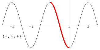
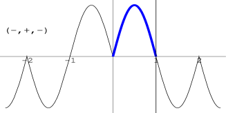
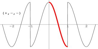
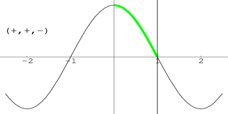
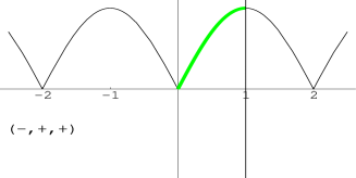
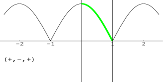
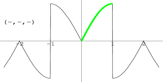
Figure 1: Eigenfunctions of $-\partial^{2}_{y}$, for a real even field $\varphi(y)$, versus $y/(\pi R)$. For each boundary condition, labelled by ($V_{0},V_{\pi},V_{\beta}$), the eigenfunction corresponding to the lightest non-vanishing mode is displayed.

Indeed, the two cases are related by a coordinate transformation and a field redefinition:

$$\varphi_{2}(y)=\epsilon(y/2)~{}\varphi_{1}(y+\pi R)~{}~{}~{}.$$ (13)

If $\varphi_{1}(y)$ is even, continuous and antiperiodic, it is easy to see that the function $\varphi_{2}(y)$ defined in (13) is even, periodic and has a cusp in $y=y_{2q}$, where it vanishes. The equations of motion are not affected by the translation $y\to y+\pi R$, which simply exchanges the boundary conditions at $y=y_{2q}$ and $y=y_{2q+1}$. Moreover, the physical properties of a quantum mechanical system are invariant under a local field redefinition. Therefore the two systems related by eq. (13) are equivalent.

In table 1 we collect spectrum and eigenvalues for all possible cases that are allowed by an even or odd field $\varphi$. We have found it useful to express the solutions in terms of the sign function, which specifies the singularities of the system. Indeed, $\epsilon(y/2)$ is singular in $y=y_{2q}$, $\epsilon(y/2+\pi R/2)$ in $y=y_{2q+1}$ and $\epsilon(y)$ in all $y=y_{q}$. The correct parity of the solutions is guaranteed by the properties of $\epsilon(y)$. Also the periodicity can be easily determined from the fact that $\epsilon(y)$ is periodic, whereas $\epsilon(y/2)$ and $\epsilon(y/2+\pi R/2)$ are antiperiodic.

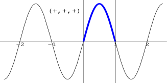
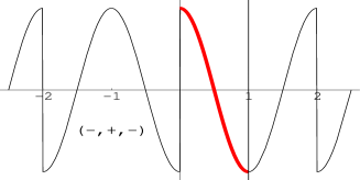
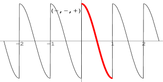
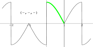
Figure 2: Eigenfunctions of $-\partial^{2}_{y}$, for a real odd field $\varphi(y)$, versus $y/(\pi R)$. For each boundary condition, labelled by ($V_{0},V_{\pi},V_{\beta}$), the eigenfunction corresponding to the lightest non-vanishing mode is displayed.

There are three types of spectra: first, the ordinary Kaluza-Klein tower $n/R$ that includes a zero mode; second, an identical spectrum with the absence of the zero mode and, finally, the Kaluza-Klein tower shifted by $1/2R$. All systems that possess the same spectrum can be related by field redefinitions that can be easily derived from table 1. The only non-trivial transformation, applying only to the case of semi-integer spectrum, is the one in (13). For semi-integer spectrum, all $\varphi_{k}$ $(k=1,...8)$ are related. For integer and non-negative spectrum, we have maps among $\varphi_{1}$, $\varphi_{3}$, $\varphi_{6}$ and $\varphi_{8}$. For strictly positive integer spectrum, $\varphi_{2}$, $\varphi_{4}$, $\varphi_{5}$ and $\varphi_{7}$ are related. Thanks to these relations, we can always go from a description in terms of discontinuous field variables to a descriptions by the smooth fields $\varphi_{1}(y)$ or $\varphi_{5}(y)$. Also, as can be seen from figs. 1 and 2, the behavior in the vicinity of the fixed points is the same for all the eigenfunctions representing the same type of spectrum, up to a possible exchange between the two fixed points. In the presence of a single real field $\varphi$ the parity $Z$ does not seem to have an absolute physical meaning. We find that there are equivalent physical systems with opposite $Z$ parities for $\varphi$.

In conclusion, there are less physically inequivalent systems than independent boundary conditions, at least for free theories. There are different boundary conditions that lead to the same spectra and the corresponding systems are related by field redefinitions. The parameter $V_{0}\cdot V_{\pi}\cdot V_{\beta}$ is equal in equivalent systems. When $V_{0}\cdot V_{\pi}\cdot V_{\beta}=+1$, $m~{}R$ is integer whereas for $V_{0}\cdot V_{\pi}\cdot V_{\beta}=-1$, $m~{}R$ is semi-integer.

4. More scalar fields

Several scalar fields lead to the possibility of exploiting continuous global symmetries to characterize boundary conditions. As an example, we consider here the case of a 5D complex scalar field $\varphi(y)\equiv(\varphi_{1}(y)+i~{}\varphi_{2}(y))/\sqrt{2}$. Its equation of motion:

$$-\partial^{2}_{y}\varphi=m^{2}\varphi~{}~{}~{},$$ (14)

is invariant under global O(2) transformations, acting on $(\varphi_{1},\varphi_{2})$.

We first discuss the case where $Z=diag(+1,-1)$ in the basis $(\varphi_{1},\varphi_{2})$. In this case we can take:

$$U_{\gamma}=\left(\begin{array}[]{cc}\cos\theta_{\gamma}&\sin\theta_{\gamma}\\ -\sin\theta_{\gamma}&\cos\theta_{\gamma}\end{array}\right)~{}~{}~{},$$ (15)

which is a symmetry of the theory and satisfies (9). In general, we can choose three independent angles $\theta_{\gamma}=(\beta,\delta_{0},\delta_{\pi})$ for the twist and the two jumps at $y=0,\pi R$ respectively. The solution of the equation of motion subjected to these boundary conditions can be obtained by the same method used in section 3. We find:

$$\varphi(y)=e^{\displaystyle i(my-\alpha(y))}~{}~{}~{},$$ (16)

where

$$m=\frac{n}{R}-\frac{(\beta-\delta_{0}-\delta_{\pi})}{2\pi R}~{}~{}~{}~{}~{}~{}~{}~{}~{}~{}(n\in Z)~{}~{}~{},$$ (17)

and

$$\alpha(y)=\frac{\delta_{0}-\delta_{\pi}}{4}~{}\epsilon(y)+\frac{\delta_{0}+\delta_{\pi}}{4}~{}\eta(y)~{}~{}~{}.$$ (18)

The function $\eta(y)$ is the ‘staircase’ function

$$\eta(y)=2q+1~{}~{}~{}~{}~{}~{}~{}~{}~{}y_{q}<y<y_{q+1}~{}~{}~{}~{}~{}~{}~{}~{}~{}~{}(q\in Z)~{}~{}~{}.$$ (19)

The function $\alpha(y)$ is flat everywhere but at $y=y_{q}$, where it jumps, leading to the desired behavior of the solution at the fixed points. It satisfies $\alpha(y+2\pi R)=\alpha(y)+\delta_{0}+\delta_{\pi}$, thus contributing to the overall twist $\beta$ of $\varphi(y)$ by the amount $\delta_{0}+\delta_{\pi}$. This explains why the shift of the spectrum with respect to the Kaluza-Klein levels is given by $\beta-\delta_{0}-\delta_{\pi}$ and not by $\beta$ as in the conventional Scherk-Schwarz mechanism.

When $\beta-\delta_{0}-\delta_{\pi}=0~{}~{}~{}({\rm mod}~{}2\pi)$, the masses are $n/R$ and we can order all massive modes in pairs. Indeed each physical non-vanishing mass $|m|=|n|/R$ $(n\neq 0)$ corresponds to two independent eigenfunctions. For instance, when $\beta=\delta_{0}=\delta_{\pi}=0$, we have $\varphi_{\pm}^{n}=\exp(\pm iny/R)$. This infinite series of degenerate 4D doublets can be interpreted as a consequence of the $O(2)$ symmetry, which is unbroken. A non-vanishing shift of the Kaluza-Klein levels induces an explicit breaking of the $O(2)$ symmetry. The order parameter is $\beta-\delta_{0}-\delta_{\pi}$ $({\rm mod}~{}2\pi)$. When $\beta-\delta_{0}-\delta_{\pi}$ is non-vanishing (and not a multiple of $2\pi$), the eigenfunctions of the massive modes are no longer paired, each of them corresponding now to a different physical mass. As for the case of a single real field, different boundary conditions may lead to the same spectrum. For instance, it is possible that $O(2)$ remains unbroken, despite the existence of non-trivial boundary conditions, if twist and jumps are such that the combination $\beta-\delta_{0}-\delta_{\pi}$ vanishes mod $2\pi$. Moreover, starting from a generic system with both twist $\beta$ and jumps $\delta_{0,\pi}$ different from zero, we can always move to an equivalent ‘smooth’ theory where the jumps vanish and the twist $\beta^{c}$ of the new scalar field $\varphi^{c}(y)$ is given by $\beta-\delta_{0}-\delta_{\pi}$. The map between the two systems is given by:

$$\varphi^{c}(y)=e^{\displaystyle{i\alpha(y)}}\varphi(y)~{}~{}~{}.$$ (20)

The multiplicative factor $e^{\displaystyle{i\alpha(y)}}$ removes the discontinuities from $\varphi(y)$ and add a twist $-\delta_{0}-\delta_{\pi}$ to the wave function.

Another interesting case is that of $Z$ proportional to the identity. If we assign the same $Z$ parity to the real components $\varphi_{1,2}(y)$, then $U_{\gamma}$ commutes with $Z$ and the condition (9) implies that its eigenvalues are $\pm 1$. If also $[U_{0},U_{\pi}]=0$, then it is not restrictive to go to a field basis where all $U_{\gamma}$ are diagonal, with elements $\pm 1$. This would lead to a discussion qualitatively close to that of section 3, where twist and jumps were quantized. A new feature occurs if $[U_{0},U_{\pi}]\neq 0$. Consider as an example $Z=U_{\beta}=diag(+1,+1)$ in the basis $(\varphi_{1},\varphi_{2})$. A consistent choice for $U_{0}$ and $U_{\pi}$ is:

$$U_{0}=\left(\begin{array}[]{cc}\cos\delta_{0}&-\sin\delta_{0}\\ -\sin\delta_{0}&-\cos\delta_{0}\end{array}\right)~{}~{}~{},~{}~{}~{}~{}~{}~{}~{}~{}~{}U_{\pi}=\left(\begin{array}[]{cc}1&0\\ 0&-1\end{array}\right)~{}~{}~{}.$$ (21)

Notice that the $O(2)$ matrices $U_{0}$ and $U_{\pi}$ square to 1, as required by the condition (9). The solutions of the equations of motion are:

$$\phi_{1}(y) = \cos(my-\alpha^{\prime}(y))$$

$$\phi_{2}(y) = \epsilon(y)\sin(my-\alpha^{\prime}(y))~{}~{}~{},$$ (22)

where

$$m=\frac{n}{R}+\frac{\delta_{0}}{2\pi R}~{}~{}~{}~{}~{}~{}~{}~{}~{}~{}(n\in Z)~{}~{}~{},$$ (23)

and

$$\alpha^{\prime}(y)=\frac{\delta_{0}}{4}~{}\left(\epsilon(y)+\eta(y)\right)~{}~{}~{}.$$ (24)

It is interesting to note that this choice of boundary conditions leads to a theory that is physically equivalent to that studied at the beginning of this section, where the fields $\varphi_{1}$ and $\varphi_{2}$ had opposite parity. We can go back to that system and consider the case of periodic fields with a jump at $y=0$: $Z=diag(+1,-1)$, $U_{\pi}=U_{\beta}=1$ and $U_{0}$ as in (15) with $\theta_{0}=\delta_{0}$. If we now perform the field redefinition:

$$\varphi_{1}(y)\to\varphi_{1}(y)~{}~{}~{},~{}~{}~{}~{}~{}~{}~{}~{}~{}~{}~{}\varphi_{2}(y)\to\epsilon(y)~{}\varphi_{2}(y)~{}~{}~{},$$ (25)

the new field variables are both even and periodic and their jumps are those given in (21). It is easy to see that also the solutions (16) are mapped into (22). Moreover, it will be now possible to describe the theory defined by the jumps (21) in terms of smooth field variables, characterized by a certain twist.

This correspondence provides another example of equivalent systems, despite a different assignment of the orbifold parity. The presence of discontinuous fields is a generic feature of field theories on orbifolds. The present discussion suggests that at least in some cases these discontinuities may not have any physical significance, being only related to a particular and not compelling choice of field variables.

5. Gauge vector bosons

Our generalized boundary conditions can be exploited to spontaneously break the gauge invariance of a 5D system. This is well-known as far as the twist is concerned. A non-trivial twist induces a shift in the Kaluza-Klein levels. This lifts the zero modes of the gauge vector bosons and the gauge symmetry, from a 4D point of view, is broken [3, 4]. As we have seen in the previous sections, also the discontinuities of the fields and their first derivatives have a similar effect on the spectrum and we may expect that, in the context of a gauge theory, they lead to spontaneous breaking of the 4D gauge invariance. To analyze these aspects, we focus on a 5D gauge theory defined on our orbifold and based on the gauge group SU(2).

Not all $Z_{2}$ parity assignments for the gauge fields $A^{a}_{M}(x,y)$ $(a=1,2,3)$, $(M=\mu,5)$, $(\mu=0,1,2,3)$ are now possible. The gauge invariance imposes several restrictions. First of all, the action of $Z_{2}$ on the 4D vector bosons $A^{a}_{\mu}$ should be compatible with the algebra of gauge group. In other words, we should embed $Z_{2}$ into the automorphism algebra of the gauge group [13]. For SU(2) this leaves two possibilities: either all $A^{a}_{\mu}$ are even, or two of them are odd and one is even. Furthermore, a well-defined parity for the field strength implies that the parity of $A^{a}_{5}$ should be opposite to that of $A^{a}_{\mu}$. In the basis $(A^{1}_{\mu},A^{2}_{\mu},A^{3}_{\mu})$, up to a re-labelling of the 3 gauge fields, we can consider:

$$({\rm A})~{}~{}~{}~{}~{}~{}~{}~{}~{}~{}~{}~{}~{}Z = diag(+1,+1,+1)$$

$$({\rm B})~{}~{}~{}~{}~{}~{}~{}~{}~{}~{}~{}~{}~{}Z = diag(-1,-1,+1)~{}~{}~{}.$$ (26)

The boundary conditions on the $A^{a}_{\mu}$ are specified by 3 by 3 matrices $U_{\gamma}$ that satisfy the consistency relation (9) and leave the SU(2) algebra invariant [8, 13]. This last requirement can be fulfilled by requiring that $U_{\gamma}$ is an SU(2) global transformation that acts on $(A^{1}_{\mu},A^{2}_{\mu},A^{3}_{\mu})$ in the adjoint representation. Finally, to preserve gauge invariance, the boundary conditions on the scalar fields $A^{a}_{5}$ should be the same as those on the corresponding 4D vector bosons. This can be seen by asking that the various components of the field strength $F^{a}_{MN}$ possess well-defined boundary conditions.

For instance, in the case (A) where all fields $A^{a}_{\mu}$ have even $Z_{2}$ parity, a consistent assignment is [11]:

$$U_{\beta}=diag(-1,-1,+1)~{}~{}~{},~{}~{}~{}~{}~{}~{}~{}~{}~{}~{}U_{0}=U_{\pi}=diag(+1,+1,+1)~{}~{}~{}.$$ (27)

In the gauge $\partial^{M}A^{a}_{M}=0$, the 5D equation of motion read:

$$-\partial^{2}_{y}A^{a}_{M}=m^{2}A^{a}_{M}~{}~{}~{}.$$ (28)

The solutions with the appropriate boundary conditions are:

$$A^{a}_{\mu}(x,y)=A^{a(n_{a})}_{\mu}(x)\cos m_{a}y~{}~{}~{}~{}~{}~{}m_{1,2}R=n_{1,2}+\frac{1}{2}~{}~{}~{}~{}~{}~{}m_{3}R=n_{3}~{}~{}~{},$$ (29)

where $n_{1,2,3}$ are non-negative integers. The only zero mode of the system is $A^{3(0)}_{\mu}(x)$ and, from a 4D point of view the original gauge symmetry is broken down to the U(1) associated to this massless gauge vector boson. The breaking of the 5D SU(2) gauge symmetry is spontaneous and each mode in (29), but $A^{3(0)}_{\mu}(x)$, becomes massive via an Higgs mechanism. The unphysical Goldstone bosons are the modes of the fields $A^{a}_{5}(x,y)$, which are all absorbed by the corresponding massive vector bosons. On the wall at $y=0$ all the gauge fields and the parameters of the gauge transformations are non-vanishing. Here all the constraints coming from the full 5D gauge invariance are effective. Instead, on the wall at $y=\pi R$, only $A^{3}_{\mu}(x,y)$ and the corresponding gauge parameter are different from zero. Therefore the effective symmetry at the fixed point $y=\pi R$ is the U(1) related to the 4D gauge boson $A^{3}_{\mu}(x,\pi R)$. This kind of setup where the gauge symmetry is broken by twisted orbifold boundary conditions and the two fixed points are characterized by two different effective 4D symmetries has recently received lot of attention, for its successful application in the context of grand unified theories [11, 12, 13, 14].

It is interesting to note that the same physical system discussed above can be described by using periodic field variables, with discontinuities at the fixed points. This is achieved, for instance, by means of the boundary conditions

$$U_{\beta}=U_{0}=diag(+1,+1,+1)~{}~{}~{},~{}~{}~{}~{}~{}~{}~{}~{}~{}~{}U_{\pi}=diag(-1,-1,+1)~{}~{}~{}.$$ (30)

The solutions to the equations of motion (28) are:

$$A^{a}_{\mu}(x,y) = A^{a(n_{a})}_{\mu}(x)~{}\epsilon(y/2+\pi R/2)\cos m_{a}y~{}~{}~{}~{}~{}~{}m_{a}R=n_{a}+\frac{1}{2}~{}~{}~{}~{}~{}~{}~{}~{}~{}~{}(a=1,2)$$

$$A^{3}_{\mu}(x,y) = A^{3(n_{3})}_{\mu}(x)\cos m_{3}y~{}~{}~{}~{}~{}~{}~{}~{}~{}~{}~{}~{}~{}~{}~{}m_{3}R=n_{3}~{}~{}~{},$$ (31)

where $n_{1,2,3}$ are non-negative integers. The new solutions $A^{1,2}_{\mu}$ have cusps at $y=y_{2q+1}$, as the profiles denoted by $(+,-,+)$ in fig. 1. The two descriptions are related by the field redefinition:

$$A^{a}_{\mu}(x,y)~{}\to~{}\epsilon(y/2+\pi R/2)~{}A^{a}_{\mu}(x,y)~{}~{}~{}~{}~{}~{}(a=1,2)~{}~{}~{}.$$ (32)

In the previous example the boundary conditions $U_{\gamma}$ commute among themselves and with the parity $Z$. As a consequence the rank of the gauge group SU(2) is conserved in the symmetry breaking. We can lower the rank by assuming $[U_{\gamma},Z]\neq 0$ [13, 14]. As an example, we consider the parity (B) of eq. (26) and boundary conditions described by:

$$U_{\gamma}=e^{\displaystyle\theta_{\gamma}T^{2}}~{}~{}~{}~{}~{}~{}~{}T^{2}=\left(\begin{array}[]{ccc}0&0&1\\ 0&0&0\\ -1&0&0\end{array}\right)~{}~{}~{},$$ (33)

in the basis $(A^{1}_{\mu},A^{2}_{\mu},A^{3}_{\mu})$. We allow, at the same time, for a twist $\theta_{\beta}\equiv\beta$ and two jumps $\theta_{0(\pi)}\equiv\delta_{0}(\delta_{\pi})$. The matrices $U_{\gamma}$ are block diagonal and do not mix the index 2 with the indices (1,3). Thus the boundary conditions are trivial for the odd field $A^{2}_{\mu}$ and its derivative. Non-trivial boundary conditions involve the fields $A^{1}_{\mu}$ and $A^{3}_{\mu}$. By solving the equations (28), we obtain:

$$A^{1}_{\mu}(x,y) = A^{(n)}_{\mu}(x)~{}\sin(my-\alpha(y))$$

$$A^{2}_{\mu}(x,y) = A^{2(n_{2})}_{\mu}(x)~{}\sin m_{2}y~{}~{}~{}~{}~{}~{}~{}~{}~{}~{}~{}~{}~{}~{}~{}~{}~{}~{}~{}~{}~{}~{}~{}m_{2}R=n_{2}~{}~{}~{}~{}$$

$$A^{3}_{\mu}(x,y) = A^{(n)}_{\mu}(x)~{}\cos(my-\alpha(y))~{}~{}~{}~{}~{}~{}~{}~{}~{}~{}~{}~{}~{}~{}~{}~{}mR=n-\frac{\beta-\delta_{0}-\delta_{\pi}}{2\pi}~{}~{}~{},$$ (34)

where $n\in Z$, $n_{2}$ is a positive integer and the function $\alpha(y)$ has been defined in eqs. (18) and (19). If $\beta-\delta_{0}-\delta_{\pi}=0$ (mod $2\pi$), we have a zero mode $A^{(0)}_{\mu}(x)$ and the gauge symmetry is spontaneously broken down to U(1), as in the previously discussed examples. When $\beta-\delta_{0}-\delta_{\pi}\neq 0$ (mod $2\pi$), there are no zero modes and SU(2) is completely broken. We can go continuously from this phase to the phase where a U(1) survives, by changing the twist and/or the jump parameters. We may thus have a situation where U(1) is broken by a very small amount, compared to the scale $1/R$ that characterizes the SU(2) breaking. The U(1) breaking order parameter is the combination $\beta-\delta_{0}-\delta_{\pi}$. The same physical system is described by a double infinity of boundary conditions, those that reproduce the same order parameter. All these descriptions are equivalent and are related by field redefinitions. In the class of all equivalent theories one of them is described by continuous fields $A^{a~{}c}_{\mu}(x,y)$. We go from the generic theory described in terms of $(\beta,\delta_{0},\delta_{\pi})$ to that characterized by $(\beta^{c}\equiv\beta-\delta_{0}-\delta_{\pi},\delta^{c}_{0}\equiv 0,\delta^{c}_{\pi}\equiv 0)$, via the field transformation:

$$\left(\begin{array}[]{c}A^{1~{}c}_{\mu}\\ A^{3~{}c}_{\mu}\end{array}\right)=\left(\begin{array}[]{cc}\cos\alpha(y)&-\sin\alpha(y)\\ \sin\alpha(y)&\cos\alpha(y)\\ \end{array}\right)\left(\begin{array}[]{c}A^{1}_{\mu}\\ A^{3}_{\mu}\end{array}\right)~{}~{}~{}.$$ (35)

6. Brane action for bosonic system

In the previous sections we showed the equivalence between bosonic systems characterized by discontinuous fields and ‘smooth’ systems in which fields are continuous but twisted. For each pair of systems characterized by the same mass spectrum we were able to find a local field redefinition, plus a possible discrete translation, mapping the mass eigenfunctions of one system into those of the other system. Here we would like to further explore the relation between smooth and discontinuous systems by showing that the field discontinuities are strictly related to lagrangian terms localized at the fixed points.

We begin by discussing the case of one real scalar field. To fix the ideas we focus on the equivalence between the cases $(+,+,-)$ and $(+,-,+)$ with $Z=1$ of table 1. The other cases can be discussed along similar lines. We denote by $\varphi^{c}$ the continuous field $(+,+,-)$ with twist $U_{\beta}=-1$ and by $\varphi$ the periodic field $(+,-,+)$ that has a jump $U_{\pi}=-1$. If we start from the Lagrangian $\mathcal{L}$ for the boson $\varphi^{c}$

$$\mathcal{L}(\varphi^{c},\partial\varphi^{c})=-\frac{1}{2}\partial_{M}\varphi^{c}\partial^{M}\varphi^{c}~{}~{}~{},$$ (36)

and we perform the field redefinition:

$$\varphi^{c}(y)=\chi(y)\varphi(y)~{}~{}~{}~{}~{}~{}~{}~{}\chi(y)\equiv\epsilon(y/2+\pi R/2)~{}~{}~{},$$ (37)

we obtain an expression in terms of discontinuous fields and their derivatives, from which it is difficult to derive the correct equation of motion for the system. Indeed the new lagrangian is highly singular and the naive use of the variational principle, which is tailored on continuous functions and smooth functionals, would lead to inconsistent results. In order to avoid these problems we regularize $\chi(y)$ by means of a smooth function $\chi_{\lambda}(y)$ ($\lambda>0$) which reproduces $\chi(y)$ in the limit $\lambda\to 0$. By performing the substitution:

$$\varphi^{c}(y)=\chi_{\lambda}(y)~{}\varphi(y)~{}~{}~{},$$ (38)

we obtain

$$\mathcal{L}(\varphi^{c},\partial\varphi^{c})=-\frac{1}{2}\chi_{\lambda}^{2}\partial_{M}\varphi\partial^{M}\varphi-\chi_{\lambda}\chi_{\lambda}^{\prime}\varphi\partial_{y}\varphi-\frac{1}{2}\chi_{\lambda}^{\prime 2}\varphi^{2}~{}~{}~{}.$$ (39)

Since the field $\varphi(y)$ is periodic, we can work in the interval $0\leq y\leq 2\pi R$. In the limit $\lambda\to 0$, we find:

$$\mathcal{L}(\varphi^{c},\partial\varphi^{c})=-\frac{1}{2}\chi^{2}\partial_{M}\varphi\partial^{M}\varphi+2\chi~{}\delta_{\pi R}~{}\varphi\partial_{y}\varphi-2\delta_{\pi R}^{2}~{}\varphi^{2}~{}~{}~{}~{}~{}~{}~{}~{}~{}y\in[0,2\pi]~{}~{}~{},$$ (40)

with $\delta_{y_{0}}\equiv\delta(y-y_{0})$.

The action contains quadratic terms for the field $\varphi(y)$ that are localized at $y=\pi R$. However these terms are quite singular and, strictly speaking, are mathematically ill-defined even as distributions. For this reason we derive the equation of motion for $\varphi(y)$ using the regularized action, eq. (39), from which we get:

$$\chi_{\lambda}\left(\chi_{\lambda}\partial_{y}^{2}\varphi+2~{}\chi_{\lambda}^{\prime}\partial_{y}\varphi+\chi_{\lambda}^{\prime\prime}\varphi+\chi_{\lambda}m^{2}\varphi\right)=0~{}~{}~{},$$ (41)

where we identified $\partial_{\mu}\partial^{\mu}\varphi$ with $m^{2}\varphi$. The term in brackets should vanish everywhere, since it is continuous and we can choose $\chi_{\lambda}(y)$ different from zero everywhere except at one point between 0 and $2\pi R$. If we finally take the limit $\lambda\to 0$ we obtain the equation of motion for the discontinuous fields:

$$\chi\partial_{y}^{2}\varphi-4\delta_{\pi R}\partial_{y}\varphi-2\delta_{\pi R}^{\prime}\varphi+\chi~{}m^{2}\varphi=0~{}~{}~{}.$$ (42)

Away from the point $y=\pi R$ this equation reduces to the equation of motion for continuous fields: terms with delta functions disappear and we can divide by $\chi(y)$. We obtain:

$$\partial_{y}^{2}\varphi+m^{2}\varphi=0~{}~{}~{}.$$ (43)

Moreover, by integrating eq. (42) and its primitive around $y=\pi R$, we find:

$$\begin{array}[]{l}\varphi(\pi R+\xi)=-\varphi(\pi R-\xi)\\ \varphi^{\prime}(\pi R+\xi)=-\varphi^{\prime}(\pi R-\xi)~{}~{}~{},\end{array}$$ (44)

which are just the expected jumps.

There is another possibility to derive the correct equation of motion from a singular action, beyond that of adopting a convenient regularization. We illustrate this procedure in the case of one complex scalar field $\varphi(y)$. The basic idea is to use a set of field variables such that their infinitesimal variations, implied by the action principle, are continuous functions of $y$. The action principle requires that the variation of the action $S$, assumed to be a smooth functional of $\varphi$ and $\partial\varphi$, vanishes for infinitesimal variations of the fields from the classical trajectory:

$$\delta S=\int d^{4}x~{}dy~{}\frac{\delta\mathcal{L}}{\delta\varphi}~{}\delta\varphi=0~{}~{}~{}.$$ (45)

If the system is described by discontinuous fields, in general we cannot demonstrate that $\delta\mathcal{L}/\delta\varphi$ vanishes at the singular points, since multiplication/division by discontinuous functions like $\delta\varphi$ is known to produce inequivalent equalities. An exception is the case of fields whose generic variation $\delta\varphi$ is a continuous function, despite the discontinuities of $\varphi$. In this case the action principle leads directly to the usual equation of motion.

We consider as an example the case discussed at the beginning of section 4. Real and imaginary components of $\varphi$ are respectively even and odd functions of $y$ and we have boundary conditions specified by the matrices $U_{\gamma}$ in eq. (15). In particular, the discontinuities of $\varphi_{i}$ $(i=1,2)$ and its $y$-derivative across 0 and $\pi R$ are given by:

$$\left(\begin{array}[]{c}\varphi_{1(2)}\\ \partial_{y}\varphi_{1(2)}\end{array}\right)(\gamma^{+})-\left(\begin{array}[]{c}\varphi_{1(2)}\\ \partial_{y}\varphi_{1(2)}\end{array}\right)(\gamma^{-})=(-)2\tan\frac{\delta_{\gamma}}{2}\left(\begin{array}[]{c}\varphi_{2(1)}\\ \partial_{y}\varphi_{2(1)}\end{array}\right)(\gamma)~{}~{}~{},$$ (46)

where $\gamma$ stands for $0$ or $\pi R$, $\gamma^{+(-)}$ denotes $0^{+(-)}$ or $\pi R^{+(-)}$ and

$$\left(\begin{array}[]{c}\varphi_{1(2)}\\ \partial_{y}\varphi_{1(2)}\end{array}\right)(\gamma)\equiv\frac{1}{2}\left[\left(\begin{array}[]{c}\varphi_{1(2)}\\ \partial_{y}\varphi_{1(2)}\end{array}\right)(\gamma^{+})+\left(\begin{array}[]{c}\varphi_{1(2)}\\ \partial_{y}\varphi_{1(2)}\end{array}\right)(\gamma^{-})\right]~{}~{}~{}.$$ (47)

¿From this we see that a generic variation of $\varphi_{2}$ is discontinuous. The jump of $\delta\varphi_{2}$ across $0$ or $\pi R$ is proportional to the value of $\delta\varphi_{1}$ at that point, which in general is not zero. However we can move to a new set of real fields $\theta$ and $\rho$:

$$\varphi=\rho~{}e^{i\theta}~{}~{}~{},$$ (48)

whose discontinuities from eq. (46) read:

$$\left(\begin{array}[]{c}\rho\\ \partial_{y}\rho\end{array}\right)(\gamma^{+})=\left(\begin{array}[]{c}\rho\\ \partial_{y}\rho\end{array}\right)(\gamma^{-})~{}~{}~{}~{}~{}~{}~{}~{}~{}~{}\left(\begin{array}[]{c}\theta\\ \partial_{y}\theta\end{array}\right)(\gamma^{+})-\left(\begin{array}[]{c}\theta\\ \partial_{y}\theta\end{array}\right)(\gamma^{-})=\left(\begin{array}[]{c}\delta_{\gamma}\\ 0\end{array}\right)~{}~{}~{}.$$ (49)

The discontinuity of $\theta$ at each fixed point is a constant, independent from the value of $\varphi$ at that point. As a consequence, the infinitesimal variation $\delta\theta$ relevant to the action principle is continuous everywhere, including the points $y=0$ and $y=\pi R$. We can derive the action for $(\rho,\theta)$, by starting from the Lagrangian expressed in terms of $\varphi^{c}\equiv\rho\exp[i(\theta+\alpha)]$, where the function $\alpha$ has been defined in eq. (18):

$$\mathcal{L}(\varphi^{c},\partial\varphi^{c})=-\partial_{M}\varphi^{c{\dagger}}\partial^{M}\varphi^{c}~{}~{}~{}.$$ (50)

In terms of $\rho$ and $\theta$ we have:

$$\mathcal{L}(\rho,\partial\rho,\theta,\partial\theta)=-\partial_{M}\rho\ \partial^{M}\rho-\rho^{2}\partial_{M}(\theta+\alpha)\ \partial^{M}(\theta+\alpha)~{}~{}~{}.$$ (51)

The Lagrangian now contains singular terms, localized at the fixed points. The equations of motions, derived from the variational principle, read:

$$\left\{\begin{array}[]{l}\partial_{M}\partial^{M}\rho-\rho\ \partial_{M}(\theta+\alpha)\ \partial^{M}(\theta+\alpha)=0\\ \partial_{M}[\rho^{2}\partial^{M}(\theta+\alpha)]=0\end{array}\right.~{}~{}~{}.$$ (52)

In the bulk $\alpha$ is constant and drops from the previous equations, which then become identical to the equations for the continuous field $\varphi^{c}$, in polar coordinates. Moreover, by integrating eq. (52) around the fixed points and by recalling the properties of the function $\alpha$, we reproduce precisely the jumps of eq. (49). The same results can be obtained by introducing a regularization for $\alpha$.

In the previous examples we have dealt with free theories. It is interesting to examine what happens when interactions are turned on. This is the case of non-abelian gauge theories. The presence of derivative interactions and discontinuous fields allows in principle localized interaction terms, that would provide a non-trivial extension of the framework considered up to now. To investigate this point we start from the 5D SU(2) Yang-Mills theory defined by $Z=diag(+1,+1,+1)$ and by the boundary conditions in eq. (27):

$$U_{\beta}=diag(-1,-1,+1)~{}~{}~{},~{}~{}~{}~{}~{}~{}~{}~{}~{}~{}U_{0}=U_{\pi}=diag(+1,+1,+1)~{}~{}~{}.$$ (53)

No jumps are present and the overall lagrangian is given only by the ‘bulk’ term:

$$\mathcal{L}=-\frac{1}{4}F^{a}_{MN}F^{aMN}~{}~{}~{}.$$ (54)

It is particularly convenient to discuss the physics in the unitary gauge, where all the would-be Goldstone bosons, eaten up by the massive Kaluza-Klein modes, vanish:

$$A_{5}^{a}(x,y)\equiv 0~{}~{}~{}~{}~{}~{}~{}(a=1,2,3)~{}~{}~{}.$$ (55)

In this gauge $F^{a}_{5\mu}\equiv\partial_{y}A^{a}_{\mu}$ and the lagrangian (54) reads:

$$\mathcal{L}=-\frac{1}{4}F^{a}_{\mu\nu}F^{a\mu\nu}-\frac{1}{2}\partial_{y}A^{a}_{\mu}\partial_{y}A^{a\mu}~{}~{}~{}.$$ (56)

To discuss the case of discontinuous gauge vector bosons, such as those associated to the boundary conditions:

$$U_{\beta}=U_{0}=diag(+1,+1,+1)~{}~{}~{},~{}~{}~{}~{}~{}~{}~{}~{}~{}~{}U_{\pi}=diag(-1,-1,+1)~{}~{}~{},$$ (57)

we can simply perform the field redefinition:

$$A^{\hat{a}}_{M}(x,y)~{}\to~{}\chi_{\lambda}(y)~{}A^{\hat{a}}_{M}(x,y)~{}~{}~{}~{}~{}~{}({\hat{a}}=1,2)~{}~{}~{},$$ (58)

where the function $\chi_{\lambda}(y)$ represents a regularized version of $\epsilon(y/2+\pi R/2)$. Such redefinition maps the twisted, smooth fields obeying (53) into periodic variables, discontinuous at $y=\pi R$, as specified in (57). Notice that this redefinition does not change the gauge condition (55). If we plug the transformation (58) into the lagrangian (56), we obtain the lagrangian for the system characterized by boundary conditions (57). We stress that, since the field redefinition (58) is local, the physics remains the same: the two systems are completely equivalent. The S-matrix elements computed with the two lagrangians are identical and, of course, this equivalence includes the non-trivial non-abelian interactions. Our aim here is only to understand how the physics, in particular the non-abelian interactions, are described by the new, discontinuous variables.

From eq. (56) we can already conclude that no localized non-abelian interaction terms arise from the field redefinition (58), in the unitary gauge. Indeed, the only term containing a $y$ derivative is quadratic, and, after the substitution (58), we will obtain terms analogous to those discussed in (39) for the case of a single scalar field. We find:

$$\mathcal{L} = -\frac{1}{4}\tilde{F}^{3}_{\mu\nu}\tilde{F}^{3\mu\nu}-\frac{1}{2}\partial_{y}A^{3}_{\mu}\partial_{y}A^{3\mu}+$$ (59)

$$+ \frac{1}{2}\chi_{\lambda}^{2}f^{3\hat{b}\hat{c}}A^{\hat{b}}_{\mu}A^{\hat{c}}_{\nu}\tilde{F}^{3\mu\nu}-\frac{1}{4}\chi_{\lambda}^{4}f^{3\hat{b}\hat{c}}f^{3\hat{d}\hat{e}}A^{\hat{b}}_{\mu}A^{\hat{c}}_{\nu}A^{\hat{d}\mu}A^{\hat{e}\nu}-$$

$$- \frac{1}{4}\chi_{\lambda}^{2}F^{\hat{a}}_{\mu\nu}F^{\hat{a}\mu\nu}-\frac{1}{2}\chi_{\lambda}^{2}\partial_{y}A^{\hat{a}}_{\mu}\partial_{y}A^{{\hat{a}}\mu}-$$

$$- \frac{1}{2}~{}\chi_{\lambda}^{\prime 2}~{}A^{\hat{a}}_{\mu}A^{\hat{a}\mu}-\chi_{\lambda}\chi_{\lambda}^{\prime}~{}A^{\hat{a}\mu}~{}\partial_{5}A^{\hat{a}}_{\mu}~{}~{}~{},$$

where $\tilde{F}^{3}_{\mu\nu}=\partial_{\mu}A^{3}_{\nu}-\partial_{\nu}A^{3}_{\mu}$, $f^{abc}$ are the structure constants of SU(2) and the indices $\hat{a},\hat{b},...$ run over 1,2. In the limit $\lambda\to 0$, the non-abelian interactions are formally unchanged, whereas the last line represents a set of localized quadratic terms. As discussed in the case of a real scalar field, such terms guarantee, via the equations of motion, that the fields obey the new boundary conditions (57). In a general gauge, interactions term localized at $y=\pi R$ are present, but they involve non-physical would-be Goldstone bosons.

To summarize, when going from a smooth to a discontinuous description of the same physical system, singular terms are generated in the lagrangian. In our free theory examples as well in the non-abelian case we have quadratic terms localized at the orbifold fixed point. Despite their highly singular behaviour, these terms are necessary for a consistent description of the system. Indeed they encode the discontinuities of the adopted field variables, which can be reproduced via the classical equation of motion, after appropriate regularization or through a careful application of the standard variational principle. Conversely, when localized terms for bulk fields are present in the 5D lagrangian, as for many phenomenological models currently discussed in the literature, the field variables are affected by discontinuities. These can be derived by analyzing the regularized equation of motion and can be crucial to discuss important physical properties of the system, such as its mass spectrum. In some case we can find a field redefinition that eliminate the discontinuities and provide a smooth description of the system.

7. Conclusion

Symmetries and their realizations are central to our understanding of particle interactions. The possibility of extending the present framework into a unified and more fundamental picture relies mostly on a realistic and consistent description of the breaking of viable symmetry candidates such as supersymmetry or grand unified symmetry.

In this respect conventional 4D field theories often appear to be quite limited. For example, it is well-known that a satisfactory 4D grand unified theory requires a rather baroque Higgs sector, to overcome the long standing problem of doublet-triplet splitting and the more recent one raised by the experimental bounds on the proton lifetime [20]. The study of field theories with extra, compactified dimensions proved to be extremely fruitful for the new possibilities offered for symmetry breaking. One of the most interesting mechanism for symmetry breaking, having no counterpart in four dimension, is that related to coordinate dependent-compactification, originally proposed by Scherk and Schwarz. The lagrangian is invariant under a certain group of transformations, which, however, are not preserved by the boundary conditions obeyed by the fields. The extension of the Scherk-Schwarz proposal to the case of orbifold compactifications has revealed several subtleties. The twist defining the boundary conditions should obey certain consistency conditions and the field variables are allowed to possess discontinuities at the orbifold fixed points, or, saying it differently, bulk fields are allowed to have lagrangian terms localized at the fixed points.

In this paper we have given a systematic discussion of bosonic fields on an extra dimension compactified on $S^{1}/Z_{2}$. We were motivated by the following questions. What kind of boundary conditions can be assigned to the fields? We have seen that the orbifold constructions allows to introduce jumps for both fields and first derivatives, characterized by certain unitary transformations. How are the boundary conditions related to the mass spectrum? We found that the mass spectrum depends on a combination of twist and jumps. Does a given physical system correspond to a unique choice of boundary conditions or can different boundary conditions give rise to the same physics? We found that there are local field redefinitions that relate different boundary conditions, turning a jump into a twist or vice-versa. Therefore, within the examples explored, an entire class of boundary conditions corresponds to the same physical system. In particular we found that, within this class, it is always possible to move to smooth field variables, where all the relevant information is encoded in the twist. When using this set of field variables, the lagrangian has only a ‘bulk’ term. As expected, localized and highly singular terms are present and actually needed when a description in terms of discontinuous variables is adopted. At least within the class of models explored here, such a description is not compulsory and the localization of the corresponding lagrangian terms has no intrinsic physical meaning.

Acknowledgements We would like to thank A. Torrielli for useful discussions and J. Bagger and F. Zwirner for discussions, suggestions and for their participation in the early stage of this work. C.B. and F.F. are partially supported by the European Programs HPRN-CT-2000-00148 and HPRN-CT-2000-00149.

References

- [1] N. Arkani-Hamed, A.G. Cohen and H. Georgi, Phys. Rev. Lett. 86 (2001) 4757; C. T. Hill, S. Pokorski and J. Wang, Phys. Rev. D 64 (2001) 105005.
- [2] L.J. Dixon, J.A. Harvey, C. Vafa and E. Witten, Nucl. Phys. B 261 (1985) 678 and Nucl. Phys. B 274 (1986) 285.
- [3] Y. Hosotani, Phys. Lett. B 126 (1983) 309 and Ann. of Phys. 190 (1989) 233.
- [4] J. Scherk and J.H. Schwarz, Nucl. Phys. B 153 (1979) 61 and Phys. Lett. B 82 (1979) 60; see also P. Fayet, Phys. Lett. B 159 (1985) 121 and Nucl. Phys. B263 (1986) 249.
- [5] L. J. Hall and C. F. Kolda, Phys. Lett. B 459 (1999) 213; H. C. Cheng, B. A. Dobrescu and C. T. Hill, Nucl. Phys. B 589 (2000) 249; H. C. Cheng, Int. J. Mod. Phys. A 16S1C (2001) 937; D. Dominici, Phys. Lett. B 500 (2001) 183; N. Arkani-Hamed, L. J. Hall, Y. Nomura, D. R. Smith and N. Weiner, Nucl. Phys. B 605, 81 (2001); H. C. Cheng, C. T. Hill and J. Wang, Phys. Rev. D 64, 095003 (2001); N. Arkani-Hamed, A. G. Cohen and H. Georgi, Phys. Lett. B 513 (2001) 232; N. Weiner, hep-ph/0106021; A. Masiero, C. A. Scrucca, M. Serone and L. Silvestrini, Phys. Rev. Lett. 87, 251601 (2001); M. Quiros, J. Phys. G 27, 2497 (2001).
- [6] A. Delgado, A. Pomarol and M. Quiros, Phys. Rev. D 60, 095008 (1999); R. Barbieri, L. J. Hall and Y. Nomura, Phys. Rev. D 63 (2001) 105007; A. Delgado and M. Quiros, Nucl. Phys. B 607 (2001) 99; V. Di Clemente, S. F. King and D. A. Rayner, Nucl. Phys. B 617 (2001) 71; R. Barbieri, G. Marandella and M. Papucci, hep-ph/0205280.
- [7] P. Candelas, G. T. Horowitz, A. Strominger and E. Witten, Nucl. Phys. B 258 (1985) 46; I. Antoniadis, C. Munoz and M. Quiros, Nucl. Phys. B 397 (1993) 515; C. Bachas, hep-th/9503030; K. Benakli, Phys. Lett. B 386 (1996) 106; I. Antoniadis, E. Dudas and A. Sagnotti, Nucl. Phys. B 544 (1999) 469; I. Antoniadis, S. Dimopoulos, A. Pomarol and M. Quiros, Nucl. Phys. B 544 (1999) 503; M. Sakamoto, M. Tachibana and K. Takenaga, Phys. Lett. B 458 (1999) 231; D. E. Kaplan, G. D. Kribs and M. Schmaltz, Phys. Rev. D 62 (2000) 035010; N. Arkani-Hamed, L. J. Hall, D. R. Smith and N. Weiner, Phys. Rev. D 63 (2001) 056003; D. E. Kaplan and T. M. Tait, JHEP 0006 (2000) 020; T. Kobayashi and K. Yoshioka, Phys. Rev. Lett. 85 (2000) 5527; M. Chaichian, A. B. Kobakhidze and M. Tsulaia, Phys. Lett. B 505 (2001) 222; D. Marti and A. Pomarol, Phys. Rev. D 64 (2001) 105025; N. Maru, N. Sakai, Y. Sakamura and R. Sugisaka, Nucl. Phys. B 616 (2001) 47; J. Bagger, F. Feruglio and F. Zwirner, JHEP 0202 (2002) 010; K. A. Meissner, H. P. Nilles and M. Olechowski, hep-th/0205166.
- [8] R. Barbieri, L. J. Hall and Y. Nomura, Nucl. Phys. B 624 (2002) 63.
- [9] See also: P. Horava and E. Witten, Nucl. Phys. B 460 (1996) 506 and Nucl. Phys. B 475 (1996) 94; P. Horava, Phys. Rev. D 54 (1996) 7561; I. Antoniadis and M. Quiros, Nucl. Phys. B 505 (1997) 109; Z. Lalak and S. Thomas, Nucl. Phys. B 515 (1998) 55; A. Lukas, B. A. Ovrut and D. Waldram, Phys. Rev. D 57 (1998) 7529 and JHEP 9904 (1999) 009; E. A. Mirabelli and M. E. Peskin, Phys. Rev. D 58, 065002 (1998); J. R. Ellis, Z. Lalak, S. Pokorski and W. Pokorski, Nucl. Phys. B 540 (1999) 149; K. A. Meissner, H. P. Nilles and M. Olechowski, Nucl. Phys. B 561 (1999) 30; A. Falkowski, Z. Lalak and S. Pokorski, Nucl. Phys. B 613 (2001) 189; T. Gherghetta and A. Riotto, Nucl. Phys. B 623 (2002) 97; G. von Gersdorff, M. Quiros and A. Riotto, hep-th/0204041.
- [10] E. Witten, Nucl. Phys. B 258 (1985) 75.
- [11] Y. Kawamura, Prog. Theor. Phys. 105 (2001) 999.
- [12] G. Altarelli and F. Feruglio, Phys. Lett. B 511 (2001) 257; L. J. Hall and Y. Nomura, Phys. Rev. D 64 (2001) 055003; A. Hebecker and J. March-Russell, Nucl. Phys. B 613 (2001) 3; R. Barbieri, L. J. Hall and Y. Nomura, hep-ph/0106190; T. j. Li, Phys. Lett. B 520 (2001) 377; C. Csaki, G. D. Kribs and J. Terning, Phys. Rev. D 65 (2002) 015004; H. C. Cheng, K. T. Matchev and J. Wang, Phys. Lett. B 521 (2001) 308; N. Haba, T. Kondo, Y. Shimizu, T. Suzuki and K. Ukai, Prog. Theor. Phys. 106 (2001) 1247; T. Asaka, W. Buchmuller and L. Covi, Phys. Lett. B 523 (2001) 199; L. J. Hall, Y. Nomura, T. Okui and D. R. Smith, Phys. Rev. D 65 (2002) 035008; T. j. Li, Nucl. Phys. B 619 (2001) 75; R. Dermisek and A. Mafi, Phys. Rev. D 65 (2002) 055002; T. Watari and T. Yanagida, Phys. Lett. B 519 (2001) 164; Y. Nomura, Phys. Rev. D 65 (2002) 085036; G. Bhattacharyya and K. Sridhar, hep-ph/0111345; C. S. Huang, J. Jiang, T. j. Li and W. Liao, Phys. Lett. B 530 (2002) 218; E. Witten, hep-ph/0201018; A. Hebecker and J. March-Russell, hep-ph/0204037; T. Asaka, W. Buchmuller and L. Covi, hep-ph/0204358; S. M. Barr and I. Dorsner, hep-ph/0205088; C. Biggio, hep-ph/0205142.
- [13] A. Hebecker and J. March-Russell, Nucl. Phys. B 625 (2002) 128.
- [14] L. J. Hall, H. Murayama and Y. Nomura, hep-th/0107245.
- [15] J. A. Bagger, F. Feruglio and F. Zwirner, Phys. Rev. Lett. 88 (2002) 101601.
- [16] H. Georgi, A. K. Grant and G. Hailu, Phys. Lett. B 506 (2001) 207; R. Contino, L. Pilo, R. Rattazzi and E. Trincherini, Nucl. Phys. B 622 (2002) 227; D. M. Ghilencea, S. Groot Nibbelink and H. P. Nilles, Nucl. Phys. B 619 (2001) 385; R. Barbieri, L. J. Hall and Y. Nomura, hep-ph/0110102; G. von Gersdorff, N. Irges and M. Quiros, hep-th/0204223; D. Marti and A. Pomarol, hep-ph/0205034.
- [17] N. Arkani-Hamed, A. G. Cohen and H. Georgi, Phys. Lett. B 516 (2001) 395; C. A. Scrucca, M. Serone, L. Silvestrini and F. Zwirner, Phys. Lett. B 525 (2002) 169; L. Pilo and A. Riotto, hep-th/0202144; R. Barbieri, R. Contino, P. Creminelli, R. Rattazzi and C. A. Scrucca, hep-th/0203039; S. Groot Nibbelink, H. P. Nilles and M. Olechowski, hep-th/0205012.
- [18] S. Ferrara, C. Kounnas and M. Porrati, Phys. Lett. B 206, 25 (1988); C. Kounnas and M. Porrati, Nucl. Phys. B 310, 355 (1988); S. Ferrara, C. Kounnas, M. Porrati and F. Zwirner, Nucl. Phys. B 318, 75 (1989).
- [19] M. Porrati and F. Zwirner, Nucl. Phys. B 326, 162 (1989); E. Dudas and C. Grojean, Nucl. Phys. B 507, 553 (1997); I. Antoniadis and M. Quiros, Nucl. Phys. B 505, 109 (1997) and Phys. Lett. B 416, 327 (1998); A. Pomarol and M. Quiros, Phys. Lett. B 438 (1998) 255.
- [20] See, for instance: G. Altarelli, F. Feruglio and I. Masina, JHEP 0011 (2000) 040.