UMTG–238

TBA boundary flows in the tricritical Ising field theory
Rafael I. Nepomechie and Changrim Ahn

Boundary $S$ matrices for the boundary tricritical Ising field theory (TIM), both with and without supersymmetry, have previously been proposed. Here we provide support for these $S$ matrices by showing that the corresponding boundary entropies are consistent with the expected boundary flows. We develop the fusion procedure for boundary RSOS models, with which we derive exact inversion identities for the TIM. We confirm the TBA description of nonsupersymmetric boundary flows of Lesage et al., and we obtain corresponding descriptions of supersymmetric boundary flows.

1 Introduction

A well-known (but nevertheless, remarkable) feature of integrable quantum field theories in $1+1$ dimensions is that their exact bulk [1] and boundary [2] scattering matrices can be found. However, such results are generally not obtained in a systematic way from the action; rather, one often relies on general principles (factorizability, unitarity, crossing, bootstrap, etc.) and educated guesses about symmetry, mass spectrum, etc. A case in point is the tricritical Ising field theory – i.e., the tricritical Ising conformal field theory (CFT) [3, 4, 5] perturbed by the $\Phi_{(1\,,3)}$ operator [6]. We shall refer to this field theory as the “tricritical Ising model ” or TIM for short. The bulk $S$ matrix was proposed in [7], and boundary $S$ matrices were proposed in [8, 9]. This field theory has several notable properties, which render it a very attractive toy model: it is unitary; it is supersymmetric; and it is one of the simplest examples of a model of massive kinks, whose scattering matrices are of RSOS [10, 11] type. Moreover, the bulk and boundary soliton $S$ matrices [12, 13] of the $N=1$ supersymmetric sine-Gordon model [14, 15] contain the corresponding TIM $S$ matrices as one of the factors.

A thermodynamic Bethe Ansatz (TBA) analysis [16] can provide a nontrivial check on a given bulk [17, 18] or boundary [19, 20, 21] scattering matrix. Indeed, the $S$ matrices serve as the input of the “TBA machinery,” whose output consists of certain data (central charge [3, 4], boundary entropy [22, 23]) which characterizes the corresponding CFT. For the TIM, a TBA check of the proposed bulk $S$ matrix [7] was performed in [18].

One of the principal aims of this paper is to perform an analogous TBA check of the boundary $S$ matrices which have been proposed in [8, 9]. Such an analysis is technically nontrivial, since neither the bulk nor boundary $S$ matrices are diagonal. As in the bulk case [18], the key step is the derivation of an exact inversion identity which is obeyed by an appropriate transfer matrix. For the boundary case considered here, the transfer matrix is of the “double-row” type [24].

A second aim of this paper is to develop the techniques for deriving the necessary inversion identity. We do this in an extended appendix, building on earlier work on fusion for vertex [25, 26, 27] and RSOS [28, 29, 30] models. The main idea is to formulate an RSOS open-chain fusion formula, and to show that the TIM fused transfer matrix is proportional to the identity matrix.

A third aim of this paper is to derive TBA descriptions of TIM massless boundary flows. Let us recall [22, 8, 9] that the tricritical Ising CFT has a discrete set of (super) conformal boundary conditions. Boundary perturbations can lead to flows among these boundary conditions [8, 31, 32, 33, 34, 9]. A TBA description of the nonsupersymmetric flows was proposed in [31] on the basis of an analogy with the Kondo problem. Here we give a derivation of that TBA result, as well as the results for supersymmetric flows not considered in [31], directly from the TIM scattering theory. (An alternative approach based on a lattice formulation of the TIM is considered in [34]. However, it seems that this approach cannot generate the boundary entropies.)

The outline of this article is as follows. In Sec. 2, we review the bulk and boundary $S$ matrices [7, 8, 9] which will serve as inputs for our TBA calculation. There are two boundary $S$ matrices that are not supersymmetric; and there are two boundary $S$ matrices which do have supersymmetry, which we call NS and R. We also briefly review the classification of (super) conformal boundary conditions, certain pairs of which are connected by boundary flows. In Sec. 3, we carry out the first step of the TBA program, which consists of constructing the so-called Yang matrix [35] and relating it to a commuting transfer matrix. For the problem at hand, we require a boundary RSOS version of the Yang matrix, which is an interesting generalization of the known case of periodic boundary conditions. In Sec. 4, we use an exact inversion identity to determine the eigenvalues of the transfer matrix in terms of roots of certain Bethe Ansatz equations. We restrict our attention here to the NS case. In Sec. 5 we use these results to derive the TBA equations and boundary entropy. Moreover, we find massless scaling limits which correspond to boundary flows, both for the NS case and the nonsupersymmetric cases. In Sec. 6 we briefly discuss the R case, which is closely related (in fact, dual) to the NS case. Our conclusions are presented in Sec. 7. In an Appendix, we give a brief account of the fusion procedure for RSOS models with boundary, and provide the derivation of the TIM inversion identity.

2 TIM scattering theory

We briefly review in this Section some pertinent results on the TIM scattering theory. We first define the bulk model as a perturbed bulk CFT, and give the bulk $S$ matrix [7]. We then enumerate the possible (super) conformal boundary conditions, and give the boundary $S$ matrices which have been proposed [8, 9] to describe certain perturbations of some of these boundary conditions. Two of the boundary $S$ matrices do not have supersymmetry, and two of them do. Many of the notations used in this paper are introduced in this Section.

2.1 Bulk

The bulk TIM is defined by the “action” [7]

$$A=A_{{\cal M}(4/5)}+\lambda\int_{-\infty}^{\infty}dy\int_{-\infty}^{\infty}dx\ \Phi_{({3\over 5}\,,{3\over 5})}(x\,,y)\,,\qquad\lambda<0\,,$$ (2.1)

where $A_{{\cal M}(4/5)}$ is the action for the tricritical Ising CFT (i.e., the minimal unitary model ${\cal M}(4/5)$ with central charge $c={7\over 10}$), and $\Phi_{({3\over 5}\,,{3\over 5})}$ is the spinless $(1\,,3)$ primary field of this CFT with dimensions $({3\over 5}\,,{3\over 5})$. Moreover, $\lambda$ is a bulk parameter with dimension length${}^{-{4\over 5}}$. We restrict our attention to the case $\lambda<0$, for which there is a three-fold vacuum degeneracy, and the spectrum consists of massive (mass $m>0$) kinks $K_{a\,,b}(\theta)$ that separate neighboring vacua, $a\,,b\in\{-1\,,0\,,1\}$ with $|a-b|=1$. Multi-kink states

$$K_{a_{1}\,,b_{1}}(\theta_{1})\ K_{a_{2}\,,b_{2}}(\theta_{2})\ldots$$

must obey the adjacency conditions $b_{1}=a_{2}\,,$ etc.

The two-kink $S$ matrix $S_{a\ b}^{c\ d}(\theta)$ is defined by the relation (see Figure 1)

$$K_{a\,,c}(\theta_{1})\ K_{c\,,b}(\theta_{2})=\sum_{d}S_{a\ b}^{c\ d}(\theta_{1}-\theta_{2})\ K_{a\,,d}(\theta_{2})\ K_{d\,,b}(\theta_{1}).$$ (2.2)

Figure 1: Bulk $S$ matrix $S_{a\ b}^{c\ d}(\theta_{1}-\theta_{2})$.

The nonzero matrix elements are given by [7, 18]

$$S_{0\ 0}^{\sigma\ \sigma^{\prime}}(\theta) = e^{-i\gamma\theta}\sigma(\theta)\ \bar{S}_{0\ 0}^{\sigma\ \sigma^{\prime}}(\theta)\,,$$

$$S_{\sigma\ \sigma^{\prime}}^{0\ 0}(\theta) = e^{i\gamma\theta}\sigma(\theta)\ \bar{S}_{\sigma\ \sigma^{\prime}}^{0\ 0}(\theta)\,,$$ (2.3)

where $\sigma\,,\sigma^{\prime}\in\{-1\,,+1\}$, $\gamma={1\over 2\pi}\ln 2$, and the “reduced” matrix elements $\bar{S}_{a\ b}^{c\ d}(\theta)$ are given by

$$\bar{S}_{0\ 0}^{\sigma\ \sigma}(\theta) = \cosh{\theta\over 4}\,,\qquad\qquad\qquad\bar{S}_{0\ \ 0}^{\sigma\ -\sigma}(\theta)=-i\sinh{\theta\over 4}\,,$$

$$\bar{S}_{\sigma\ \sigma}^{0\ 0}(\theta) = \sqrt{2}\cosh{1\over 4}(\theta-i\pi)\,,\qquad\bar{S}_{\sigma\ -\sigma}^{0\ \ 0}(\theta)=\sqrt{2}\cosh{1\over 4}(\theta+i\pi)\,.$$ (2.4)

Finally, $\sigma(\theta)$ is a function which obeys

$$\sigma(\theta)=\sigma(i\pi-\theta)\,,\qquad\sigma(\theta)\ \sigma(-\theta)={1\over\cosh{\theta\over 2}}\,,$$ (2.5)

and has no poles in the physical strip $0\leq\Im m\ \theta<\pi$. A useful integral representation for this function is

$$\sigma(\theta)={-i\over\sqrt{2}\sinh({1\over 4}(\theta-i\pi))}\exp\left(i\int_{0}^{\infty}{dt\over t}{\sin({\theta t\over\pi})\sinh({3t\over 2})\over\sinh(2t)\cosh({t\over 2})}\right)\,.$$ (2.6)

This is a “reduction” of the well-known integral representation for the factor $U(\theta)$ of the sine-Gordon $S$ matrix [1] with ${8\pi\over\gamma^{\prime}}={1\over 4}$.

Zamolodchikov has shown in [7] that this $S$ matrix “commutes” with supersymmetry charges $Q$ and $\bar{Q}$, which obey the $N=1$ supersymmetry algebra with topological charge. The $S$ matrix also commutes with the spin-reversal operator $\Gamma$, which is defined by

$$\Gamma\ K_{a_{1}\,,a_{2}}(\theta_{1})\ K_{a_{2}\,,a_{3}}(\theta_{2})\ldots K_{a_{N}\,,a_{N+1}}(\theta_{N})$$ (2.7)

$$=K_{-a_{1}\,,-a_{2}}(\theta_{1})\ K_{-a_{2}\,,-a_{3}}(\theta_{2})\ldots K_{-a_{N}\,,-a_{N+1}}(\theta_{N})\,.$$

Further properties of the $S$ matrix are listed in Appendix A.

2.2 Boundary

Although the three vacua $-1\,,0\,,+1$ are degenerate in the bulk, these vacua do not necessarily remain degenerate at the boundary. Chim [8] has identified the six conformal boundary conditions (CBC) [22] of the tricritical Ising CFT as follows: for the boundary conditions $(-)\,,(0)\,,(+)$, the order parameter is fixed at the boundary to the vacua $-1\,,0\,,+1$, respectively. For the boundary condition $(-0)$, the vacua $-1$ and $0$ are degenerate at the boundary; hence, the order parameter at the boundary may be in either of these two vacua. Similarly, for the boundary condition $(0+)$, the $0$ and $+1$ vacua are degenerate at the boundary. Finally, for the boundary condition $(d)$, all three vacua $-1\,,0\,,+1$ are degenerate at the boundary (as well as in the bulk); i.e., the order parameter at the boundary may be in any of the three vacua. The corresponding $g$ factors [23] are given by [8]

$$g_{(d)} = \sqrt{2}\eta^{2}C\,,\qquad g_{(-0)}=g_{(0+)}=\eta^{2}C\,,$$

$$g_{(0)} = \sqrt{2}C\,,\qquad g_{(-)}=g_{(+)}=C\,,$$ (2.8)

where

$$C=\sqrt{{\sin{\pi\over 5}}\over{\sqrt{5}}}\,,\qquad\eta=\sqrt{{\sin{{2\pi}\over 5}}\over{\sin{\pi\over 5}}}\,.$$ (2.9)

It is argued in [9] that the conformal boundary conditions $(-)\&(+)$, $(-0)\&(0+)$, $(0)$ and $(d)$ are in fact superconformal. Notice that the first two of these superconformal boundary conditions correspond to superpositions of “pure” Cardy states.

We shall consider separately integrable perturbations of both conformal and superconformal boundary conditions, resulting in models without and with supersymmetry, respectively. We assume [8] that also in the perturbed theory the boundary can have (at most) three possible states, corresponding to the three different vacua, which are created by the boundary operator $B_{a}$ with $a\in\{-1\,,0\,,1\}$. Multi-kink states have the form

$$K_{a_{1}\,,a_{2}}(\theta_{1})\ K_{a_{2}\,,a_{3}}(\theta_{2})\ldots K_{a_{N}\,,a}(\theta_{N})\ B_{a}\,.$$

The kink boundary $S$ matrix $R\!\begin{array}[]{l}{\ \ \scriptstyle{c}}\\ {\scriptstyle{a}}\\ {\ \ \scriptstyle{b}}\end{array}(\theta)$ is defined by the relation (see Figure 2)

$$K_{a\,,b}(\theta)\ B_{b}=\sum_{c}R\!\begin{array}[]{l}{\ \ \scriptstyle{c}}\\ {\scriptstyle{a}}\\ {\ \ \scriptstyle{b}}\end{array}(\theta)\ K_{a\,,c}(-\theta)\ B_{c}\,.$$ (2.13)

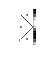
Figure 2: Boundary $S$ matrix $R\!\begin{array}[]{l}{\ \ \scriptstyle{c}}\\ {\scriptstyle{a}}\\ {\ \ \scriptstyle{b}}\end{array}(\theta)$.

2.2.1 Non-supersymmetric cases

Chim [8] has considered the TIM on the half-line $x\leq 0$ corresponding to an integrable perturbation of the CBC $(-0)$. The model is defined by the action

$$A = A_{{\cal M}(4/5)+(-0)}+\lambda\int_{-\infty}^{\infty}dy\int_{-\infty}^{0}dx\ \Phi_{({3\over 5}\,,{3\over 5})}(x\,,y)$$ (2.14)

$$- h\int_{-\infty}^{\infty}dy\ \phi_{({3\over 5})\,,(-0)}(y)\,,\qquad\lambda<0\,.$$

The last term is the boundary perturbation. It involves the boundary primary field $\phi_{({3\over 5})\,,(-0)}$ with dimension $\Delta_{(1\,,3)}={3\over 5}$ which acts on the CBC $(-0)$. Moreover, $h$ is a boundary parameter which has dimensions length${}^{-{2\over 5}}$.

The boundary $S$ matrix which has been proposed [8] for this model has the following nonzero matrix elements

$$R\!\begin{array}[]{l}{\ \ \scriptstyle{-1}}\\ {\scriptstyle{0}}\\ {\ \ \scriptstyle{-1}}\end{array}(\theta\,,\xi) = P(\theta\,,\xi)\ \bar{R}\!\begin{array}[]{l}{\ \ \scriptstyle{-1}}\\ {\scriptstyle{0}}\\ {\ \ \scriptstyle{-1}}\end{array}(\theta\,,\xi)\,,$$ (2.21)

$$R\!\begin{array}[]{l}{\ \ \scriptstyle{0}}\\ {\scriptstyle{\sigma}}\\ {\ \ \scriptstyle{0}}\end{array}(\theta\,,\xi) = M(\theta\,,\xi)\ \bar{R}\!\begin{array}[]{l}{\ \ \scriptstyle{0}}\\ {\scriptstyle{\sigma}}\\ {\ \ \scriptstyle{0}}\end{array}(\theta\,,\xi)\,,$$ (2.28)

where the reduced matrix elements $\bar{R}\!\begin{array}[]{l}{\ \ \scriptstyle{c}}\\ {\scriptstyle{a}}\\ {\ \ \scriptstyle{b}}\end{array}(\theta\,,\xi)$ are given by

$$\bar{R}\!\begin{array}[]{l}{\ \ \scriptstyle{-1}}\\ {\scriptstyle{0}}\\ {\ \ \scriptstyle{-1}}\end{array}(\theta\,,\xi) = 1\,,$$ (2.32)

$$\bar{R}\!\begin{array}[]{l}{\ \ \scriptstyle{\ 0}}\\ {\scriptstyle{\pm 1}}\\ {\ \ \scriptstyle{\ 0}}\end{array}(\theta\,,\xi) = \cos{\xi\over 2}\pm i\sinh{\theta\over 2}\,.$$ (2.36)

The parameter $\xi$ is related in some way to the boundary parameter $h$ appearing in the action (2.14). The function $P(\theta\,,\xi)$ is given by

$$P(\theta\,,\xi)=P^{CDD}(\theta\,,\xi)\ P_{min}(\theta)\,,$$ (2.37)

where $P^{CDD}(\theta\,,\xi)$ is the CDD factor

$$P^{CDD}(\theta\,,\xi)={\sin\xi-i\sinh\theta\over\sin\xi+i\sinh\theta}\,,$$ (2.38)

which has a pole at $\theta=i\xi$, and $P_{min}(\theta)$ is the minimal solution of the equations

$$P_{min}(\theta)P_{min}(-\theta)=1\,,\quad P_{min}({i\pi\over 2}-\theta)=\sqrt{2}e^{2i\gamma\theta}\cosh({\theta\over 2}-{i\pi\over 4})\sigma(2\theta)P_{min}({i\pi\over 2}+\theta)\,,$$ (2.39)

with no poles in the physical strip $0\leq\Im m\ \theta<{\pi\over 2}$. We find that it has the integral representation

$$P_{min}(\theta)=\exp i\left(-\gamma\theta+{1\over 8}\int_{0}^{\infty}{dt\over t}{\sin({2\theta t\over\pi})\over\cosh^{2}t\cosh^{2}{t\over 2}}\right)\,.$$ (2.40)

Finally, the function $M(\theta\,,\xi)$ is given by

$$M(\theta\,,\xi)=e^{2i\gamma\theta}\sigma(\theta-i\xi)\ \sigma(\theta+i\xi)\ P(\theta\,,\xi)\,.$$ (2.41)

There is a similar model corresponding to a perturbation of the CBC $(0+)$. The boundary $S$ matrix for this case is the same as the one given above, except that $R\!\begin{array}[]{l}{\ \ \scriptstyle{-1}}\\ {\scriptstyle{0}}\\ {\ \ \scriptstyle{-1}}\end{array}(\theta\,,\xi)=0$, and

$$R\!\begin{array}[]{l}{\ \ \scriptstyle{1}}\\ {\scriptstyle{0}}\\ {\ \ \scriptstyle{1}}\end{array}(\theta\,,\xi)=P(\theta\,,\xi)\ \bar{R}\!\begin{array}[]{l}{\ \ \scriptstyle{1}}\\ {\scriptstyle{0}}\\ {\ \ \scriptstyle{1}}\end{array}(\theta\,,\xi)\,,$$ (2.48)

with $\bar{R}\!\begin{array}[]{l}{\ \ \scriptstyle{1}}\\ {\scriptstyle{0}}\\ {\ \ \scriptstyle{1}}\end{array}(\theta\,,\xi)=1$. Neither of these two models has supersymmetry.

2.2.2 Supersymmetric cases

Supersymmetric perturbations of the tricritical Ising boundary CFT with two different superconformal boundary conditions (namely, $(-0)\&(0+)$ and $(d)$) are considered in [9]. We refer to these two cases as NS and R, respectively, since these are the sectors to which the corresponding boundary states belong.

NS case

The NS case corresponds to a perturbation of the boundary condition $(-0)\&(0+)$, with action

$$A = A_{{\cal M}(4/5)+(-0)\&(0+)}+\lambda\int_{-\infty}^{\infty}dy\int_{-\infty}^{0}dx\ \Phi_{({3\over 5}\,,{3\over 5})}(x\,,y)$$ (2.49)

$$- h\int_{-\infty}^{\infty}dy\ \left(\phi_{({3\over 5})\,,(-0)}(y)-\phi_{({3\over 5})\,,(0+)}(y)\right)\,,\qquad\lambda<0\,.$$

The proposed boundary $S$ matrix is the “direct sum” of the boundary $S$ matrices given in Sec. 2.2.1 for the perturbations of $(-0)$ and $(0+)$. That is, the nonzero matrix elements are given by

$$R\!\begin{array}[]{l}{\ \ \scriptstyle{\sigma}}\\ {\scriptstyle{0}}\\ {\ \ \scriptstyle{\sigma}}\end{array}(\theta\,,\xi) = P(\theta\,,\xi)\ \bar{R}\!\begin{array}[]{l}{\ \ \scriptstyle{\sigma}}\\ {\scriptstyle{0}}\\ {\ \ \scriptstyle{\sigma}}\end{array}(\theta\,,\xi)\,,$$ (2.56)

$$R\!\begin{array}[]{l}{\ \ \scriptstyle{0}}\\ {\scriptstyle{\sigma}}\\ {\ \ \scriptstyle{0}}\end{array}(\theta\,,\xi) = M(\theta\,,\xi)\ \bar{R}\!\begin{array}[]{l}{\ \ \scriptstyle{0}}\\ {\scriptstyle{\sigma}}\\ {\ \ \scriptstyle{0}}\end{array}(\theta\,,\xi)\,,$$ (2.63)

where

$$\bar{R}\!\begin{array}[]{l}{\ \ \scriptstyle{\sigma}}\\ {\scriptstyle{0}}\\ {\ \ \scriptstyle{\sigma}}\end{array}(\theta\,,\xi) = 1\,,$$ (2.67)

$$\bar{R}\!\begin{array}[]{l}{\ \ \scriptstyle{\ 0}}\\ {\scriptstyle{\pm 1}}\\ {\ \ \scriptstyle{\ 0}}\end{array}(\theta\,,\xi) = \cos{\xi\over 2}\pm i\sinh{\theta\over 2}\,,$$ (2.71)

and the functions $P(\theta\,,\xi)$ and $M(\theta\,,\xi)$ are given by Eqs. (2.37) and (2.41), respectively. This boundary $S$ matrix “commutes” with the supersymmetry charge

$$\hat{Q}=Q+\bar{Q}+2\cos({\xi\over 2})\sqrt{m}\ \Gamma\,,$$ (2.72)

where $\Gamma$ is the spin-reversal operator (2.7).

R case

For the R case, which corresponds to a perturbation of the boundary condition $(d)$, the action is given by the image of (2.49) under duality transformation. The proposed boundary $S$ matrix has the following nonzero matrix elements

$$R\!\begin{array}[]{l}{\ \ \scriptstyle{\sigma}}\\ {\scriptstyle{0}}\\ {\ \ \scriptstyle{\sigma}}\end{array}(\theta\,,\xi) = N(\theta\,,\xi)\ \bar{R}\!\begin{array}[]{l}{\ \ \scriptstyle{\sigma}}\\ {\scriptstyle{0}}\\ {\ \ \scriptstyle{\sigma}}\end{array}(\theta\,,\xi)\,,$$ (2.79)

$$R\!\begin{array}[]{l}{\ \ \scriptstyle{-\sigma}}\\ {\scriptstyle{0}}\\ {\ \ \scriptstyle{\ \sigma}}\end{array}(\theta\,,\xi) = N(\theta\,,\xi)\ \bar{R}\!\begin{array}[]{l}{\ \ \scriptstyle{-\sigma}}\\ {\scriptstyle{0}}\\ {\ \ \scriptstyle{\ \sigma}}\end{array}(\theta\,,\xi)\,,$$ (2.86)

$$R\!\begin{array}[]{l}{\ \ \scriptstyle{0}}\\ {\scriptstyle{\sigma}}\\ {\ \ \scriptstyle{0}}\end{array}(\theta\,,\xi) = R(\theta\,,\xi)\ \bar{R}\!\begin{array}[]{l}{\ \ \scriptstyle{0}}\\ {\scriptstyle{\sigma}}\\ {\ \ \scriptstyle{0}}\end{array}(\theta\,,\xi)\,,$$ (2.93)

where the reduced matrix elements $\bar{R}\!\begin{array}[]{l}{\ \ \scriptstyle{c}}\\ {\scriptstyle{a}}\\ {\ \ \scriptstyle{b}}\end{array}(\theta\,,\xi)$ are given by

$$\bar{R}\!\begin{array}[]{l}{\ \ \scriptstyle{\sigma}}\\ {\scriptstyle{0}}\\ {\ \ \scriptstyle{\sigma}}\end{array}(\theta\,,\xi) = \cos{\xi\over 2}\,,$$ (2.97)

$$\bar{R}\!\begin{array}[]{l}{\ \ \scriptstyle{-1}}\\ {\scriptstyle{0}}\\ {\ \ \scriptstyle{+1}}\end{array}(\theta\,,\xi) = -ir\sinh{\theta\over 2}\,,\qquad\bar{R}\!\begin{array}[]{l}{\ \ \scriptstyle{+1}}\\ {\scriptstyle{0}}\\ {\ \ \scriptstyle{-1}}\end{array}(\theta\,,\xi)=-{i\over r}\sinh{\theta\over 2}\,,$$ (2.104)

$$\bar{R}\!\begin{array}[]{l}{\ \ \scriptstyle{0}}\\ {\scriptstyle{\sigma}}\\ {\ \ \scriptstyle{0}}\end{array}(\theta\,,\xi) = 1\,,$$ (2.108)

and $r$ is a parameter which presumably is related in some way to the boundary parameter $h$, as is $\xi$. Moreover, the functions $N(\theta\,,\xi)$ and $R(\theta\,,\xi)$ are given by

$$N(\theta\,,\xi) = e^{-2i\gamma\theta}M(\theta\,,\xi)\,,$$

$$R(\theta\,,\xi) = e^{2i\gamma\theta}P(\theta\,,\xi)\,.$$ (2.109)

This boundary $S$ matrix “commutes” with the supersymmetry charge

$$\hat{Q}=Q-\bar{Q}+{4ir\over 1-r^{2}}\cos({\xi\over 2})\sqrt{m}\ \Gamma\,.$$ (2.110)

In contrast to the NS case, here the matrix $R\!\begin{array}[]{l}{\ \ \scriptstyle{c}}\\ {\scriptstyle{a}}\\ {\ \ \scriptstyle{b}}\end{array}(\theta\,,\xi)$ does not vanish for $b\neq c$; i.e., it is not “diagonal.”

The parameter $r$ can be set to unity by an appropriate gauge transformation [2] of the kink operators, which corresponds to adding a total derivative term to the boundary action that restores spin-reversal symmetry. This limiting case, for which the supersymmetry charge (2.110) reduces to $\Gamma$, was considered earlier in [8].

3 Yang matrix and transfer matrix

The first step of the TBA program is to formulate the “Yang matrix” [35] and relate it to an appropriate commuting transfer matrix. Since it is not obvious how to do this for the case of boundaries, we begin by reviewing the case [18] of periodic boundary conditions.

3.1 Closed-chain transfer matrix

Following [18], we consider $N$ kinks of mass $m$ with real rapidities $\theta_{1}\,,\ldots\,,\theta_{N}$ and two-kink $S$ matrix $S_{a\ b}^{c\ d}(\theta)$ in a periodic box of length $L>>{1\over m}$. We impose the periodicity condition

$$e^{iLm\sinh\theta_{1}}K_{a_{1}\,,a_{2}}(\theta_{1})K_{a_{2}\,,a_{3}}(\theta_{2})\ldots K_{a_{N-1}\,,a_{N}}(\theta_{N-1})K_{a_{N}\,,a_{1}}(\theta_{N})$$ (3.1)

$$=K_{a_{2}\,,a_{3}}(\theta_{2})\ldots K_{a_{N}\,,a_{1}}(\theta_{N})K_{a_{1}\,,a_{2}}(\theta_{1})\,.$$

Commuting the kink operator $K_{a_{1}\,,a_{2}}(\theta_{1})$ on the LHS past the others using the relation (2.2), we obtain

$$e^{iLm\sinh\theta_{1}}\sum_{d_{2}\,,\ldots\,,d_{N}}\Big{\{}S_{a_{1}\ a_{3}}^{a_{2}\ d_{2}}(\theta_{1}-\theta_{2})S_{d_{2}\ a_{4}}^{a_{3}\ d_{3}}(\theta_{1}-\theta_{3})\ldots S_{d_{N-2}\ a_{N}}^{a_{N-1}\ d_{N-1}}(\theta_{1}-\theta_{N-1})S_{d_{N-1}\ a_{1}}^{a_{N}\ \ d_{N}}(\theta_{1}-\theta_{N})$$

$$K_{a_{1}\,,d_{2}}(\theta_{2})K_{d_{2}\,,d_{3}}(\theta_{3})\ldots K_{a_{N-1}\,,d_{N}}(\theta_{N})K_{d_{N}\,,a_{1}}(\theta_{1})\Big{\}}=K_{a_{2}\,,a_{3}}(\theta_{2})\ldots K_{a_{N}\,,a_{1}}(\theta_{N})K_{a_{1}\,,a_{2}}(\theta_{1})\,.$$

Multiplying both sides by the “wavefunction” $\Psi^{a_{1}\ldots a_{N}}$, summing over $a_{1}\,,\ldots\,,a_{N}$, and relabeling indices appropriately, we obtain the Yang equation for kink 1

$$e^{iLm\sinh\theta_{1}}\sum_{a^{\prime}_{1}\,,\ldots\,,a^{\prime}_{N}}Y_{(1)\ a^{\prime}_{1}\ldots a^{\prime}_{N}}^{\ \ \ a_{1}\ldots a_{N}}\ \Psi^{a^{\prime}_{1}\ldots a^{\prime}_{N}}=\Psi^{a_{1}\ldots a_{N}}\,,$$ (3.3)

where $Y_{(1)}$ is the Yang matrix

$$Y_{(1)\ a^{\prime}_{1}\ldots a^{\prime}_{N}}^{\ \ \ a_{1}\ldots a_{N}}=\delta^{a_{2}}_{a^{\prime}_{1}}S_{a_{2}\ a^{\prime}_{3}}^{a^{\prime}_{2}\ a_{3}}(\theta_{1}-\theta_{2})S_{a_{3}\ a^{\prime}_{4}}^{a^{\prime}_{3}\ a_{4}}(\theta_{1}-\theta_{3})\ldots S_{a_{N-1}\ a^{\prime}_{N}}^{a^{\prime}_{N-1}\ a_{N}}(\theta_{1}-\theta_{N-1})S_{a_{N}\ a_{2}}^{a^{\prime}_{N}\ a_{1}}(\theta_{1}-\theta_{N})\,.$$ (3.4)

There are similar equations, and corresponding matrices $Y_{(k)}$, for the other kinks $k=2\,,3\,,\ldots\,,N$.

The objective is to diagonalize $Y_{(k)}$. The key to this problem is to relate $Y_{(k)}$ to an inhomogeneous closed-chain transfer matrix, for which there are well-developed diagonalization techniques. To this end, we consider the transfer matrix

$$\tau_{a^{\prime}_{1}\ldots a^{\prime}_{N}}^{a_{1}\ldots a_{N}}(\theta|\theta_{1}\,,\ldots\,,\theta_{N})=S_{a_{1}\ a^{\prime}_{2}}^{a^{\prime}_{1}\ a_{2}}(\theta-\theta_{1})S_{a_{2}\ a^{\prime}_{3}}^{a^{\prime}_{2}\ a_{3}}(\theta-\theta_{2})\ldots S_{a_{N-1}\ a^{\prime}_{N}}^{a^{\prime}_{N-1}\ a_{N}}(\theta-\theta_{N-1})S_{a_{N}\ a^{\prime}_{1}}^{a^{\prime}_{N}\ a_{1}}(\theta-\theta_{N})\,,$$ (3.5)

with inhomogeneities $\theta_{1}\,,\ldots\,,\theta_{N}$. Because the $S$ matrix satisfies the Yang-Baxter equation (A.5), the transfer matrix commutes for different values of $\theta$

$$\left[\tau(\theta|\theta_{1}\,,\ldots\,,\theta_{N})\,,\tau(\theta^{\prime}|\theta_{1}\,,\ldots\,,\theta_{N})\right]=0\,.$$ (3.6)

Let us now evaluate this transfer matrix at $\theta=\theta_{1}$. Using the fact that the $S$ matrix at zero rapidity is given by (A.6), we immediately obtain $\tau(\theta_{1}|\theta_{1}\,,\ldots\,,\theta_{N})=Y_{(1)}$. In general, we have

$$Y_{(k)}=\tau(\theta_{k}|\theta_{1}\,,\ldots\,,\theta_{N})\,,\qquad k=1\,,\ldots\,,N\,.$$ (3.7)

This is the sought-after relation. In order to diagonalize the Yang matrices $Y_{(k)}$, it suffices to diagonalize the commuting closed-chain transfer matrix $\tau(\theta|\theta_{1}\,,\ldots\,,\theta_{N})$. That calculation, as well as the corresponding bulk TBA analysis, is described for the TIM in [18].

3.2 Open-chain transfer matrix

We turn now to the case with boundaries, which is our primary interest here. We therefore consider $N$ kinks of mass $m$ with real, positive rapidities $\theta_{1}\,,\ldots\,,\theta_{N}$ in an interval of length $L>>{1\over m}$, with bulk $S$ matrix $S_{a\ b}^{c\ d}(\theta)$ and boundary $S$ matrix $R\!\begin{array}[]{l}{\ \ \scriptstyle{c}}\\ {\scriptstyle{a}}\\ {\ \ \scriptstyle{b}}\end{array}(\theta\,,\xi)$. In analogy with (3.1), we propose the formal relation

$$e^{2iLm\sinh\theta_{1}}B_{a_{1}}^{+}\ K_{a_{1}\,,a_{2}}(\theta_{1})K_{a_{2}\,,a_{3}}(\theta_{2})\ldots K_{a_{N-1}\,,a_{N}}(\theta_{N-1})K_{a_{N}\,,a_{N+1}}(\theta_{N})\ B_{a_{N+1}}^{-}$$ (3.8)

$$=B_{a_{1}}^{+}\ K_{a_{1}\,,a_{2}}(\theta_{1})K_{a_{2}\,,a_{3}}(\theta_{2})\ldots K_{a_{N-1}\,,a_{N}}(\theta_{N-1})K_{a_{N}\,,a_{N+1}}(\theta_{N})\ B_{a_{N+1}}^{-}\,,$$

where now there are two boundary operators $B_{a}^{\pm}$ corresponding to the left and right boundaries, with (cf, Eq. (2.13))

$$K_{a\,,b}(\theta)\ B_{b}^{-} = \sum_{c}R\!\begin{array}[]{l}{\ \ \scriptstyle{c}}\\ {\scriptstyle{a}}\\ {\ \ \scriptstyle{b}}\end{array}(\theta\,,\xi_{-})\ K_{a\,,c}(-\theta)\ B_{c}^{-}\,,$$ (3.12)

$$B_{b}^{+}\ K_{b\,,a}(\theta) = \sum_{c}B_{c}^{+}\ K_{c\,,a}(-\theta)\ R\!\begin{array}[]{l}{\ \ \scriptstyle{c}}\\ {\scriptstyle{a}}\\ {\ \ \scriptstyle{b}}\end{array}(-\theta\,,\xi_{+})\,.$$ (3.16)

Note that for each boundary operator $B_{a}^{\pm}$ there is a corresponding boundary parameter $\xi_{\pm}$. By moving the kink operator with rapidity $\theta_{1}$ on the LHS of (3.8) to the far right using (2.2), reflecting it from the right boundary using (3.12), moving it to the far left using again (2.2), and finally reflecting it from the left boundary using (3.16), we arrive at the Yang equation for kink 1

$$e^{2iLm\sinh\theta_{1}}\sum_{a^{\prime}_{1}\,,\ldots\,,a^{\prime}_{N+1}}Y_{(1)\ a^{\prime}_{1}\ldots a^{\prime}_{N+1}}^{\ \ \ a_{1}\ldots a_{N+1}}\ \Psi^{a^{\prime}_{1}\ldots a^{\prime}_{N+1}}=\Psi^{a_{1}\ldots a_{N+1}}\,,$$ (3.17)

where the Yang matrix $Y_{(1)}$ is given by

$$Y_{(1)\ a^{\prime}_{1}\ldots a^{\prime}_{N+1}}^{\ \ \ a_{1}\ldots a_{N+1}} = \sum_{d_{2}\,,\ldots\,,d_{N}}\Big{\{}R\!\begin{array}[]{l}{\ \ \scriptstyle{a_{1}}}\\ {\scriptstyle{a_{2}}}\\ {\ \ \scriptstyle{a^{\prime}_{1}}}\end{array}(\theta_{1}\,,\xi_{+})\ S_{a^{\prime}_{1}\ a^{\prime}_{3}}^{a^{\prime}_{2}\ d_{2}}(\theta_{1}-\theta_{2})\ldots S_{d_{N-1}\ a^{\prime}_{N+1}}^{a^{\prime}_{N}\ \ \ d_{N}}(\theta_{1}-\theta_{N})$$ (3.21)

$$\times R\!\begin{array}[]{l}{\ \ \scriptstyle{a_{N+1}}}\\ {\scriptstyle{d_{N}}}\\ {\ \ \scriptstyle{a^{\prime}_{N+1}}}\end{array}(\theta_{1}\,,\xi_{-})\ S_{d_{N-1}\ a_{N+1}}^{d_{N}\ \ \ a_{N}}(\theta_{1}+\theta_{N})\ldots S_{a^{\prime}_{1}\ a_{3}}^{d_{2}\ a_{2}}(\theta_{1}+\theta_{2})\Big{\}}\,.$$ (3.25)

There are similar matrices $Y_{(k)}$ for the other kinks. In analogy with the case of periodic boundary conditions, the key to diagonalizing the Yang matrix is to relate it to an inhomogeneous open-chain transfer matrix

$$t_{a^{\prime}_{1}\ldots a^{\prime}_{N+1}}^{a_{1}\ldots a_{N+1}}(\theta|\theta_{1}\,,\ldots\,,\theta_{N}) = \sum_{a^{\prime\prime}_{1}\,,\ldots\,,a^{\prime\prime}_{N+1}}\Big{\{}R\!\begin{array}[]{l}{\ \ \scriptstyle{a_{1}}}\\ {\scriptstyle{a^{\prime\prime}_{1}}}\\ {\ \ \scriptstyle{a^{\prime}_{1}}}\end{array}(i\pi-\theta\,,\xi_{+})\ S_{a^{\prime\prime}_{1}\ a^{\prime}_{2}}^{a^{\prime}_{1}\ a^{\prime\prime}_{2}}(\theta-\theta_{1})\ldots S_{a^{\prime\prime}_{N}\ a^{\prime}_{N+1}}^{a^{\prime}_{N}\ a^{\prime\prime}_{N+1}}(\theta-\theta_{N})$$ (3.29)

$$\times R\!\begin{array}[]{l}{\ \ \scriptstyle{\ a_{N+1}}}\\ {\scriptstyle{a^{\prime\prime}_{N+1}}}\\ {\ \ \scriptstyle{\ a^{\prime}_{N+1}}}\end{array}(\theta\,,\xi_{-})\ S_{a^{\prime\prime}_{N}\ a_{N+1}}^{a^{\prime\prime}_{N+1}\ a_{N}}(\theta+\theta_{N})\ldots S_{a^{\prime\prime}_{1}\ a_{2}}^{a^{\prime\prime}_{2}\ a_{1}}(\theta+\theta_{1})\Big{\}}\,,$$ (3.33)

which commutes for different values of $\theta$

$$\left[t(\theta|\theta_{1}\,,\ldots\,,\theta_{N})\,,t(\theta^{\prime}|\theta_{1}\,,\ldots\,,\theta_{N})\right]=0\,.$$ (3.34)

The transfer matrix (3.33) is an RSOS version [13, 29, 30] of the Sklyanin [24] vertex-type transfer matrix. Using the relations (A.6), (A.21) and (A.2), one can show that

$$Y_{(k)}=t(\theta_{k}|\theta_{1}\,,\ldots\,,\theta_{N})\,,\qquad k=1\,,\ldots\,,N\,.$$ (3.35)

Hence, in order to diagonalize the Yang matrices $Y_{(k)}$, it suffices to diagonalize the open-chain transfer matrix $t(\theta|\theta_{1}\,,\ldots\,,\theta_{N})$. Indeed, let $\Psi(\theta_{1}\,,\ldots\,,\theta_{N})$ be an eigenvector of the transfer matrix with corresponding eigenvalue $\Lambda(\theta|\theta_{1}\,,\ldots\,,\theta_{N})$,

$$t(\theta|\theta_{1}\,,\ldots\,,\theta_{N})\ \Psi(\theta_{1}\,,\ldots\,,\theta_{N})=\Lambda(\theta|\theta_{1}\,,\ldots\,,\theta_{N})\ \Psi(\theta_{1}\,,\ldots\,,\theta_{N})\,.$$ (3.36)

The eigenvector is independent of $\theta$ by virtue of the commutativity property (3.34). With the help of the result (3.35), the Yang equation (3.17) implies

$$e^{2iLm\sinh\theta_{k}}\Lambda(\theta_{k}|\theta_{1}\,,\ldots\,,\theta_{N})=1\,,\qquad k=1\,,\ldots\,,N\,.$$ (3.37)

4 Inversion identity and transfer-matrix eigenvalues: NS case

We turn now to the problem of determining the eigenvalues of the inhomogeneous open-chain transfer matrix (3.33). As for the closed chain [18], our approach is to derive an exact inversion identity. For definiteness, we treat here the NS case. (See Sec. 2.2.2.) The results for the R case, which are closely related to those for the NS case, are presented in Sec. 6.

Instead of working with the full (“dressed”) transfer matrix (3.33), it is convenient (see Footnote 6 below) to work instead with the reduced (“bare”) transfer matrix $\bar{t}$, which is constructed from the reduced bulk and boundary $S$ matrices,

$$\bar{t}_{a^{\prime}_{1}\ldots a^{\prime}_{N+1}}^{a_{1}\ldots a_{N+1}}(\theta|\theta_{1}\,,\ldots\,,\theta_{N}) = \sum_{a^{\prime\prime}_{1}\,,\ldots\,,a^{\prime\prime}_{N+1}}\Big{\{}\bar{R}\!\begin{array}[]{l}{\ \ \scriptstyle{a_{1}}}\\ {\scriptstyle{a^{\prime\prime}_{1}}}\\ {\ \ \scriptstyle{a^{\prime}_{1}}}\end{array}(i\pi-\theta\,,\xi_{+})\ \bar{S}_{a^{\prime\prime}_{1}\ a^{\prime}_{2}}^{a^{\prime}_{1}\ a^{\prime\prime}_{2}}(\theta-\theta_{1})\ldots\bar{S}_{a^{\prime\prime}_{N}\ a^{\prime}_{N+1}}^{a^{\prime}_{N}\ a^{\prime\prime}_{N+1}}(\theta-\theta_{N})$$ (4.4)

$$\times \bar{R}\!\begin{array}[]{l}{\ \ \scriptstyle{\ a_{N+1}}}\\ {\scriptstyle{a^{\prime\prime}_{N+1}}}\\ {\ \ \scriptstyle{\ a^{\prime}_{N+1}}}\end{array}(\theta\,,\xi_{-})\ \bar{S}_{a^{\prime\prime}_{N}\ a_{N+1}}^{a^{\prime\prime}_{N+1}\ a_{N}}(\theta+\theta_{N})\ldots\bar{S}_{a^{\prime\prime}_{1}\ a_{2}}^{a^{\prime\prime}_{2}\ a_{1}}(\theta+\theta_{1})\Big{\}}\,.$$ (4.8)

It is also convenient to define the following four “sectors”:

$$N=\mbox{ even }-\mbox{ Sector }I : a_{1}\,,a^{\prime}_{1}\,,a_{N+1}\,,a^{\prime}_{N+1}\in\{-1\,,+1\}\,,$$

$$N=\mbox{ even }-\mbox{ Sector }II : a_{1}=a^{\prime}_{1}=a_{N+1}=a^{\prime}_{N+1}=0\,,$$

$$N=\mbox{ odd }-\mbox{ Sector }I : a_{1}\,,a^{\prime}_{1}\in\{-1\,,+1\}\,,\qquad a_{N+1}=a^{\prime}_{N+1}=0\,,$$

$$N=\mbox{ odd }-\mbox{ Sector }II : a_{1}=a^{\prime}_{1}=0\,,\qquad a_{N+1}\,,a^{\prime}_{N+1}\in\{-1\,,+1\}\,.$$ (4.9)

The nonzero matrix elements of the transfer matrix lie exclusively in these sectors. For a given parity of $N$ (i.e., even or odd), the transfer matrix decomposes into two blocks along the diagonal corresponding to sectors I and II. For the NS case (2.63), (2.71), the relation between the full transfer matrix and the reduced transfer matrix is given by

$$t^{(\alpha)}(\theta|\theta_{1}\,,\ldots\,,\theta_{N})=w^{(\alpha)}(\theta)\ \bar{t}^{(\alpha)}(\theta|\theta_{1}\,,\ldots\,,\theta_{N})\,,$$ (4.10)

where $\alpha$ runs over the four sectors (4.9), and $w^{(\alpha)}(\theta)$ is given by

$$w^{(\alpha)}(\theta)=\prod_{j=1}^{N}\sigma(\theta-\theta_{j})\sigma(\theta+\theta_{j})\times\left\{\begin{array}[]{l}P(i\pi-\theta\,,\xi_{+})\ P(\theta\,,\xi_{-})\\ M(i\pi-\theta\,,\xi_{+})\ M(\theta\,,\xi_{-})\\ e^{-2i\gamma\theta}P(i\pi-\theta\,,\xi_{+})\ M(\theta\,,\xi_{-})\\ e^{2i\gamma\theta}M(i\pi-\theta\,,\xi_{+})\ P(\theta\,,\xi_{-})\end{array}\right.\,,$$ (4.15)

respectively. The latter can be brought to the form

$$w^{(\alpha)}(\theta)={1\over\sigma(2\theta)\cosh{\theta\over 2}}\prod_{j=1}^{N}\sigma(\theta-\theta_{j})\sigma(\theta+\theta_{j})\times\left\{\begin{array}[]{l}e^{2i\gamma\theta}P(\theta\,,\xi_{+})\ P(\theta\,,\xi_{-})\\ {1\over 2}e^{-2i\gamma\theta}M(\theta\,,\xi_{+})\ M(\theta\,,\xi_{-})\\ P(\theta\,,\xi_{+})\ M(\theta\,,\xi_{-})\\ {1\over 2}M(\theta\,,\xi_{+})\ P(\theta\,,\xi_{-})\end{array}\right.$$ (4.20)

with the help of the crossing properties (2.5), (2.39).

Using the fusion procedure, we show in Appendix B that the reduced transfer matrix obeys the inversion identity

$$\bar{t}^{(\alpha)}(\theta|\theta_{1}\,,\ldots\,,\theta_{N})\ \bar{t}^{(\alpha)}(\theta+i\pi|\theta_{1}\,,\ldots\,,\theta_{N})=f^{(\alpha)}(\theta)\ \mathbb{I}^{(\alpha)}\,,$$ (4.21)

where $\alpha$ runs over the four sectors (4.9), and $f^{(\alpha)}(\theta)$ is given by

$$f^{(\alpha)}(\theta) = {1\over\cosh\theta}\Big{[}f^{(\alpha)}_{+}(\theta)\cosh^{2}{\theta\over 2}\prod_{j=1}^{N}\cosh({1\over 2}(\theta-\theta_{j}))\cosh({1\over 2}(\theta+\theta_{j}))$$ (4.22)

$$+ f^{(\alpha)}_{-}(\theta)\sinh^{2}{\theta\over 2}\prod_{j=1}^{N}\sinh({1\over 2}(\theta-\theta_{j}))\sinh({1\over 2}(\theta+\theta_{j}))\Big{]}\,,$$

where

$$f^{(\alpha)}_{\pm}(\theta)=\left\{\begin{array}[]{c}1\\ (\cosh\theta\pm\cos\xi_{-})(\cosh\theta\pm\cos\xi_{+})\\ {1\over 2}(\cosh\theta\pm\cos\xi_{-})\\ 2(\cosh\theta\pm\cos\xi_{+})\end{array}\right.\,,$$ (4.27)

respectively. This inversion identity is one of the main results of this paper. We have checked it explicitly up to $N=4$.

In addition to the inversion identity, we can establish certain further properties of the transfer matrix which are needed to determine its eigenvalues. Namely, periodicity

$$\bar{t}(\theta+2i\pi|\theta_{1}\,,\ldots\,,\theta_{N})=\bar{t}(\theta|\theta_{1}\,,\ldots\,,\theta_{N})\,,$$ (4.28)

crossing

$$\bar{t}(i\pi-\theta|\theta_{1}\,,\ldots\,,\theta_{N})=\bar{t}(\theta|\theta_{1}\,,\ldots\,,\theta_{N})\,,$$ (4.29)

and asymptotic behavior for large $\theta$

$$\bar{t}^{(\alpha)}(\theta|\theta_{1}\,,\ldots\,,\theta_{N})\sim z^{(\alpha)}(\theta)\ \mathbb{I}^{(\alpha)}\quad\mbox{ for }\quad\theta\rightarrow\infty\,,$$ (4.30)

where $\alpha$ runs over the four sectors (4.9), and $z^{(\alpha)}$ is given by

$$z^{(\alpha)}(\theta)=\left\{\begin{array}[]{l}\left(-{ie^{\theta}\over 4}\right)^{N\over 2}(\delta_{a_{1}\,,a_{N+1}}-\delta_{a_{1}\,,-a_{N+1}})\\ 2\left(-{ie^{\theta}\over 4}\right)^{{N\over 2}+1}\\ \left(-{ie^{\theta}\over 4}\right)^{N+1\over 2}(\delta_{a_{1}\,,-1}-\delta_{a_{1}\,,1})\\ 2\left(-{ie^{\theta}\over 4}\right)^{N+1\over 2}(\delta_{a_{N+1}\,,-1}-\delta_{a_{N+1}\,,1})\end{array}\right.\,,$$ (4.35)

respectively.

Acting with the above relations on an eigenvector $\Psi(\theta_{1}\,,\ldots\,,\theta_{N})$ of the (reduced) transfer matrix

$$\bar{t}(\theta|\theta_{1}\,,\ldots\,,\theta_{N})\ \Psi(\theta_{1}\,,\ldots\,,\theta_{N})=\bar{\Lambda}(\theta|\theta_{1}\,,\ldots\,,\theta_{N})\ \Psi(\theta_{1}\,,\ldots\,,\theta_{N})\,,$$ (4.36)

we obtain corresponding relations for the eigenvalues $\bar{\Lambda}^{(\alpha)}(\theta|\theta_{1}\,,\ldots\,,\theta_{N})$ in the various sectors,

$$\bar{\Lambda}^{(\alpha)}(\theta|\theta_{1}\,,\ldots\,,\theta_{N})\ \bar{\Lambda}^{(\alpha)}(\theta+i\pi|\theta_{1}\,,\ldots\,,\theta_{N}) = f^{(\alpha)}(\theta)\,,$$ (4.37)

$$\bar{\Lambda}^{(\alpha)}(\theta+2i\pi|\theta_{1}\,,\ldots\,,\theta_{N}) = \bar{\Lambda}^{(\alpha)}(\theta|\theta_{1}\,,\ldots\,,\theta_{N})\,,$$ (4.38)

$$\bar{\Lambda}^{(\alpha)}(i\pi-\theta|\theta_{1}\,,\ldots\,,\theta_{N}) = \bar{\Lambda}^{(\alpha)}(\theta|\theta_{1}\,,\ldots\,,\theta_{N})\,,$$ (4.39)

$$\bar{\Lambda}^{(\alpha)}(\theta|\theta_{1}\,,\ldots\,,\theta_{N}) \sim z^{(\alpha)}(\theta)\quad\mbox{ for }\quad\theta\rightarrow\infty\,.$$ (4.40)

The periodicity, crossing and asymptotic behavior requirements of the eigenvalues (4.38) - (4.40) are fulfilled by the Ansatz

$$\bar{\Lambda}^{(\alpha)}(\theta|\theta_{1}\,,\ldots\,,\theta_{N})=c^{(\alpha)}\prod_{j=1}^{d^{(\alpha)}}(-i)\sinh({1\over 2}(\theta-u_{j}))\cosh({1\over 2}(\theta+u_{j}))\,,$$ (4.41)

where $c^{(\alpha)}$ and $d^{(\alpha)}$ are given by

$$c^{(\alpha)}=\left\{\begin{array}[]{c}\pm 1\\ 2\\ \pm 1\\ \pm 2\end{array}\right.\,,\qquad d^{(\alpha)}=\left\{\begin{array}[]{c}{N\over 2}\\ {N\over 2}+1\\ {N+1\over 2}\\ {N+1\over 2}\end{array}\right.\,,$$ (4.50)

respectively. The parameters $\{u_{j}\}$ appearing in the Ansatz (4.41) are evidently roots of the eigenvalues, $\bar{\Lambda}^{(\alpha)}(u_{j}|\theta_{1}\,,\ldots\,,\theta_{N})=0$. It follows from the inversion identity (4.37) that $\{u_{j}\}$ are also roots of the function $f^{(\alpha)}(\theta)$, i.e., $f^{(\alpha)}(u_{j})=0$. We conclude from (4.22) that $\{u_{j}\}$ are solutions of the set of equations

$$-{f^{(\alpha)}_{-}(u_{j})\over f^{(\alpha)}_{+}(u_{j})}{\sinh^{2}{u_{j}\over 2}\over\cosh^{2}{u_{j}\over 2}}\prod_{k=1}^{N}{\sinh({1\over 2}(u_{j}-\theta_{k}))\over\cosh({1\over 2}(u_{j}-\theta_{k}))}{\sinh({1\over 2}(u_{j}+\theta_{k}))\over\cosh({1\over 2}(u_{j}+\theta_{k}))}=1\,,\qquad j=1\,,\ldots\,,d^{(\alpha)}\,,$$ (4.51)

to which we refer as “Bethe Ansatz” equations.

The periodicity property (4.38) implies that we can restrict the roots $u_{j}$ of $\bar{\Lambda}^{(\alpha)}(\theta)$ to the interval

$$-\pi<\Im m\ u_{j}\leq\pi\,.$$ (4.52)

We now demonstrate that all the roots $u_{j}$ have the form $x_{j}\pm{i\pi\over 2}$ with $x_{j}$ real. Indeed, we observe that $f^{(\alpha)}(\theta)$ has the properties

$$\left[f^{(\alpha)}(\theta)\right]^{*}=f^{(\alpha)}(\theta^{*})\,,\qquad f^{(\alpha)}(\theta\mp i\pi)=f^{(\alpha)}(\theta)\,,$$ (4.53)

where ^∗ denotes complex conjugation. These two properties imply that if $u_{j}$ is a root of $f^{(\alpha)}(\theta)$, then so are $u_{j}^{*}$ and $u_{j}\mp i\pi$, respectively. Since $u_{j}^{*}\neq u_{j}$, then $u_{j}^{*}=u_{j}\mp i\pi$. Hence, $\Im m\ u_{j}=\pm{i\pi\over 2}$.

In view of the above, we set

$$u_{j}=x_{j}+{i\pi\over 2}\epsilon_{j}\,,$$ (4.54)

with $x_{j}$ real and $\epsilon_{j}=\pm 1$. The eigenvalues (4.41) are specified by $\{x_{j}\,,\epsilon_{j}\}\,,\quad j=1\,,\ldots\,,d^{(\alpha)}$, similarly to the bulk case [18]. Hence, we can rewrite the expression for the eigenvalues as

$$\bar{\Lambda}^{(\alpha)}(\theta|\theta_{1}\,,\ldots\,,\theta_{N})=c^{(\alpha)}\prod_{j=1}^{d^{(\alpha)}}\lambda^{(1)}_{\epsilon_{j}}(\theta-x_{j})\ \lambda^{(2)}_{\epsilon_{j}}(\theta+x_{j})\,,$$ (4.55)

where

$$\lambda^{(1)}_{\epsilon}(\theta)=\sinh{1\over 2}(\theta-{i\pi\over 2}\epsilon)\,,\qquad\lambda^{(2)}_{\epsilon}(\theta)=-i\cosh{1\over 2}(\theta+{i\pi\over 2}\epsilon)\,.$$ (4.56)

Moreover, we can rewrite the Bethe Ansatz equations (4.51) in terms of $x_{j}$ (they do not depend on $\epsilon_{j}$) as

$${\cal Q}^{(\alpha)}(x_{j}\,,\xi_{\pm}){\sinh^{2}({x_{j}\over 2}-{i\pi\over 4})\over\sinh^{2}({x_{j}\over 2}+{i\pi\over 4})}\prod_{k=1}^{N}\left[-{\sinh({x_{j}-\theta_{k}\over 2}-{i\pi\over 4})\over\sinh({x_{j}-\theta_{k}\over 2}+{i\pi\over 4})}{\sinh({x_{j}+\theta_{k}\over 2}-{i\pi\over 4})\over\sinh({x_{j}+\theta_{k}\over 2}+{i\pi\over 4})}\right]=1\,,$$

$$j=1\,,\ldots\,,d^{(\alpha)}\,,$$ (4.57)

where

$${\cal Q}^{(\alpha)}(x_{j}\,,\xi_{\pm})=\left\{\begin{array}[]{c}1\\ Q(x_{j}\,,\xi_{-})\ Q(x_{j}\,,\xi_{+})\\ Q(x_{j}\,,\xi_{-})\\ Q(x_{j}\,,\xi_{+})\end{array}\right.\,,$$ (4.62)

and

$$Q(x\,,\xi)={\sinh x-i\cos\xi\over\sinh x+i\cos\xi}\,.$$ (4.63)

(As always, $\alpha$ runs over the four sectors (4.9).) Notice that (4.57) is invariant under $x_{j}\mapsto-x_{j}$. Moreover, following [37, 38], we assume that the root $x_{j}=0$ corresponds to an eigenvector with zero norm. Hence, we restrict to solutions with $x_{j}>0$.

To summarize this Section, the eigenvalues (3.36) of the full transfer matrix for the NS case of the TIM are given by

$$\Lambda^{(\alpha)}(\theta|\theta_{1}\,,\ldots\,,\theta_{N})=w^{(\alpha)}(\theta)\ \bar{\Lambda}^{(\alpha)}(\theta|\theta_{1}\,,\ldots\,,\theta_{N})\,,$$ (4.64)

where $w^{(\alpha)}(\theta)$ is given by (4.20), $\bar{\Lambda}^{(\alpha)}(\theta|\theta_{1}\,,\ldots\,,\theta_{N})$ is given by (4.55), and $\{x_{j}\}$ are positive solutions of the Bethe Ansatz equations (4.57).

5 TBA analysis

Having obtained the eigenvalues of the transfer matrix and the Bethe Ansatz equations, we can proceed to the derivation of the corresponding TBA equations and boundary entropy. Following [2, 19] we consider the partition function $Z_{+-}$ of the system on a cylinder of length $L$ and circumference $R$ with left/right boundary conditions denoted by $\pm$. It is given by

$$Z_{+-} = \mathop{\rm tr}\nolimits e^{-RH_{+-}}=e^{-RF}$$ (5.1)

$$= \langle B_{+}|e^{-LH_{P}}|B_{-}\rangle$$

$$\approx \langle B_{+}|0\rangle\langle 0|B_{-}\rangle e^{-LE_{0}}\qquad\mbox{ for }L\rightarrow\infty\,.$$

In the first line, Euclidean time evolves along the circumference of the cylinder, and $H_{+-}$ is the Hamiltonian for the system with spatial boundary conditions $\pm$. In the second line, time evolves parallel to the axis of the cylinder, $H_{P}$ is the Hamiltonian for the system with periodic boundary conditions, and $|B_{\pm}\rangle$ are boundary states which encode initial/final (temporal) conditions. In the third line, we consider the limit $L\rightarrow\infty$; the state $|0\rangle$ is the ground state of $H_{P}$, and $E_{0}$ is the corresponding eigenvalue. The quantity $\ln\langle B_{+}|0\rangle\langle 0|B_{-}\rangle$ is the sought-after boundary entropy [23, 19]. Taking the logarithm of the above expressions for the partition function, one obtains

$$-RF\approx-LE_{0}+\ln\langle B_{+}|0\rangle\langle 0|B_{-}\rangle\,.$$ (5.2)

Whereas the free energy $F$ has a leading contribution which is of order $L$, we seek here the subleading correction which is of order $1$.

5.1 Thermodynamic limit

We proceed to compute $F$ using the TBA approach [16]-[21]. To this end, we introduce the densities $P_{\pm}(\theta)$ of “magnons”, i.e., of real Bethe Ansatz roots $\{x_{j}\}$ with $\epsilon_{j}=\pm 1$, respectively; and also the densities $\rho_{1}(\theta)$ and $\tilde{\rho}(\theta)$ of particles $\{\theta_{k}\}$ and holes, respectively. Computing the imaginary part of the logarithmic derivative of the “magnonic” Bethe Ansatz equations (4.57), we obtain

$$P_{+}(\theta)+P_{-}(\theta) = {1\over 2\pi}\int_{0}^{\infty}d\theta^{\prime}\ \rho_{1}(\theta^{\prime})\left[\Phi(\theta-\theta^{\prime})+\Phi(\theta+\theta^{\prime})\right]$$ (5.3)

$$+ {1\over 2\pi L}\left[\Phi(\theta)+\Psi_{\xi_{+}}(\theta)+\Psi_{\xi_{-}}(\theta)\right]\,,$$

where

$$\Phi(\theta) = {\partial\over\partial\theta}\Im m\ \ln\left({\sinh({\theta\over 2}-{i\pi\over 4})\over\sinh({\theta\over 2}+{i\pi\over 4})}\right)={1\over\cosh\theta}\,,$$

$$\Psi_{\xi}(\theta) = {\partial\over\partial\theta}\Im m\ \ln Q(\theta\,,\xi)={4\cos\xi\cosh\theta\over\cos 2\xi+\cosh 2\theta}\,.$$ (5.4)

In the final equality, we have used the expression (4.63) for $Q(\theta\,,\xi)$, and we have assumed that $\xi$ is real. We present here the results for $N=$ even - Sector II, from which the results for the other sectors (see (4.62)) can be read off by inspection. Defining $\rho_{1}(\theta)$ for negative values of $\theta$ to be equal to $\rho_{1}(|\theta|)$, we obtain the final form

$$P_{+}(\theta)+P_{-}(\theta)={1\over 2\pi}\left(\rho_{1}*\Phi\right)(\theta)+{1\over 2\pi L}\left[\Phi(\theta)+\Psi_{\xi_{+}}(\theta)+\Psi_{\xi_{-}}(\theta)\right]\,,$$ (5.5)

where $*$ denotes convolution

$$\left(f*g\right)(\theta)=\int_{-\infty}^{\infty}d\theta^{\prime}\ f(\theta-\theta^{\prime})g(\theta^{\prime})\,.$$ (5.6)

Computing the imaginary part of the logarithmic derivative of the Yang equation (3.37) using the result (4.64) for the eigenvalue, we obtain (again for $N=$ even - Sector II)

$$\rho_{1}(\theta) + \tilde{\rho}(\theta)={1\over 2\pi}\Big{\{}2m\cosh\theta+\int_{0}^{\infty}d\theta^{\prime}\ \rho_{1}(\theta^{\prime})\left[\Phi_{\sigma}(\theta-\theta^{\prime})+\Phi_{\sigma}(\theta+\theta^{\prime})\right]$$ (5.7)

$$+ \int_{0}^{\infty}d\theta^{\prime}\ \Big{[}P_{+}(\theta^{\prime})\left(\Phi^{(1)}_{+}(\theta-\theta^{\prime})+\Phi_{+}^{(2)}(\theta+\theta^{\prime})\right)+P_{-}(\theta^{\prime})\left(\Phi^{(1)}_{-}(\theta-\theta^{\prime})+\Phi_{-}^{(2)}(\theta+\theta^{\prime})\right)\Big{]}$$

$$+ {1\over L}\left[-2\gamma-\Phi_{\sigma}(\theta)-2\Phi_{\sigma}(2\theta)+{\partial\over\partial\theta}\Im m\ \ln M(\theta\,,\xi_{+})+{\partial\over\partial\theta}\Im m\ \ln M(\theta\,,\xi_{-})\right]\Big{\}}\,,$$

where

$$\Phi_{\sigma}(\theta) = {\partial\over\partial\theta}\Im m\ \ln\sigma(\theta)={1\over 8}\int_{-\infty}^{\infty}dk\ {e^{ik\theta}\over\cosh^{2}{\pi k\over 2}}={\theta\over 2\pi\sinh\theta}\,,$$

$$\Phi_{\pm}^{(l)}(\theta) = {\partial\over\partial\theta}\Im m\ \ln\lambda^{(l)}_{\pm}(\theta)\,,\quad l=1\,,2\,,$$ (5.8)

and $\lambda^{(l)}_{\pm}(\theta)$ are introduced in (4.56). Using the facts $\Phi_{\pm}^{(1)}(\theta)=\Phi_{\pm}^{(2)}(\theta)=\pm{1\over 2}\Phi(\theta)$, and defining $P_{\pm}(\theta)$ for negative values of $\theta$ to be equal to $P_{\pm}(|\theta|)$, we obtain

$$\rho_{1}(\theta) + \tilde{\rho}(\theta)={m\over\pi}\cosh\theta+{1\over 2\pi}\left(\rho_{1}*\Phi_{\sigma}\right)(\theta)+{1\over 4\pi}\left((P_{+}-P_{-})*\Phi\right)(\theta)$$ (5.9)

$$+ {1\over 2\pi L}\left[-2\gamma-\Phi_{\sigma}(\theta)-2\Phi_{\sigma}(2\theta)+{\partial\over\partial\theta}\Im m\ \ln M(\theta\,,\xi_{+})+{\partial\over\partial\theta}\Im m\ \ln M(\theta\,,\xi_{-})\right]\,.$$

Using (5.5) to eliminate $P_{-}$, and (2.37), (2.41) to separate the various factors in $M(\theta\,,\xi)$, we obtain

$$\rho_{1}(\theta)+\tilde{\rho}(\theta) = {m\over\pi}\cosh\theta+{1\over 2\pi}P_{+}*\Phi+{1\over 2\pi}\rho_{1}*\left(\Phi_{\sigma}-{1\over 4\pi}\Phi*\Phi\right)$$

$$+ {1\over 2\pi L}\Bigg{[}2\left({\partial\over\partial\theta}\Im m\ \ln P_{min}(\theta)-\Phi_{\sigma}(2\theta)-\Phi_{\sigma}(\theta)+\gamma\right)+\left(\Phi_{\sigma}-{1\over 4\pi}\Phi*\Phi\right)$$

$$+ \left(\Phi_{\sigma}(\theta-i\xi_{+})+\Phi_{\sigma}(\theta+i\xi_{+})-{1\over 4\pi}\Psi_{\xi_{+}}*\Phi\right)$$

$$+ \left(\Phi_{\sigma}(\theta-i\xi_{-})+\Phi_{\sigma}(\theta+i\xi_{-})-{1\over 4\pi}\Psi_{\xi_{-}}*\Phi\right)$$

$$+ {\partial\over\partial\theta}\Im m\ \ln P^{CDD}(\theta\,,\xi_{+})+{\partial\over\partial\theta}\Im m\ \ln P^{CDD}(\theta\,,\xi_{-})\Bigg{]}\,.$$

Using the identity [18]

$$\Phi_{\sigma}(\theta)-{1\over 4\pi}\left(\Phi*\Phi\right)(\theta)=0\,,$$ (5.11)

as well as the identities

$$\Phi_{\sigma}(\theta-i\xi)+\Phi_{\sigma}(\theta+i\xi)-{1\over 4\pi}\left(\Psi_{\xi}*\Phi\right)(\theta) = 0\,,$$

$${\partial\over\partial\theta}\Im m\ \ln P_{min}(\theta)-\Phi_{\sigma}(2\theta)-\Phi_{\sigma}(\theta)+\gamma = -{1\over 4}\Phi(\theta)\,,$$ (5.12)

we arrive at the final simple result

$$\rho_{1}(\theta)+\tilde{\rho}(\theta)={m\over\pi}\cosh\theta+{1\over 2\pi}\left(P_{+}*\Phi\right)(\theta)+{1\over 2\pi L}\Bigg{[}-{1\over 2}\Phi(\theta)+\kappa_{\xi_{+}}(\theta)+\kappa_{\xi_{-}}(\theta)\Bigg{]}\,,$$ (5.13)

where

$$\kappa_{\xi}(\theta)={\partial\over\partial\theta}\Im m\ \ln P^{CDD}(\theta\,,\xi)={4\sin\xi\cosh\theta\over\cos 2\xi-\cosh 2\theta}\,.$$ (5.14)

The result (5.13) holds in fact for all four sectors.

The thermodynamic limit of the magnonic Bethe Ansatz equations and the Yang equations, given by (5.5) and (5.13), respectively, are the main results of this subsection.

5.2 TBA equations and boundary entropy

The free energy $F$ is given by

$$F=E-TS\,,$$ (5.15)

where the temperature is $T={1\over R}$, the energy $E$ is

$$E=\sum_{k=1}^{N}m\cosh\theta_{k}={L\over 2}\int_{-\infty}^{\infty}d\theta\ \rho_{1}(\theta)m\cosh\theta\,,$$ (5.16)

and the entropy $S$ is [16, 18]

$$S = {L\over 2}\int_{-\infty}^{\infty}d\theta\ \Big{\{}(\rho_{1}+\tilde{\rho})\ln(\rho_{1}+\tilde{\rho})-\rho_{1}\ln\rho_{1}-\tilde{\rho}\ln\tilde{\rho}$$ (5.17)

$$+ (P_{+}+P_{-})\ln(P_{+}+P_{-})-P_{+}\ln P_{+}-P_{-}\ln P_{-}\Big{\}}\,.$$

Extremizing the free energy $(\delta F=0)$ subject to the constraints

$$\delta P_{-}=-\delta P_{+}+{1\over 2\pi}\delta\rho_{1}*\Phi\,,\qquad\delta\tilde{\rho}=-\delta\rho_{1}+{1\over 2\pi}\delta P_{+}*\Phi\,,$$ (5.18)

(which follow from Eqs. (5.5), (5.13), respectively) we obtain a set of TBA equations which is the same as for the case of periodic boundary conditions [18]

$$\mathfrak{r}\cosh\theta = \epsilon_{1}(\theta)+{1\over 2\pi}\left(\Phi*L_{2}\right)(\theta)\,,$$

$$0 = \epsilon_{2}(\theta)+{1\over 2\pi}\left(\Phi*L_{1}\right)(\theta)\,,$$ (5.19)

where

$$L_{i}(\theta) = \ln\left(1+e^{-\epsilon_{i}(\theta)}\right)\,,\qquad\mathfrak{r}=mR\,,$$

$$\epsilon_{1} = \ln\left({\tilde{\rho}\over\rho_{1}}\right)\,,\qquad\epsilon_{2}=\ln\left({P_{-}\over P_{+}}\right)\,.$$ (5.20)

We next evaluate $F$ using also the constraints (5.5), (5.13) and the TBA equations. From the boundary (order $1$) contribution, we obtain (see Eq. (5.2)) the boundary entropy

$$\ln\langle B_{+}|0\rangle\langle 0|B_{-}\rangle = {1\over 4\pi}\int_{-\infty}^{\infty}d\theta\ \Big{\{}\left[-{1\over 2}\Phi(\theta)+\kappa_{\xi_{+}}(\theta)+\kappa_{\xi_{-}}(\theta)\right]L_{1}(\theta)$$ (5.26)

$$+ \left[\Phi(\theta)+\Psi_{\xi_{+}}(\theta)+\Psi_{\xi_{-}}(\theta)\right]L_{2}(\theta)\Big{\}}\,.$$

In particular, the dependence of the boundary entropy of a single boundary on the boundary parameter $\xi$ is given by

$$\ln g(\xi)={1\over 4\pi}\int_{-\infty}^{\infty}d\theta\ \left[\kappa_{\xi}(\theta)\ L_{1}(\theta)+\Psi_{\xi}(\theta)\ L_{2}(\theta)\right]\,,$$ (5.27)

where the kernels $\kappa_{\xi}(\theta)$ and $\Psi_{\xi}(\theta)$ are given in Eqs. (5.14) and (5.4), respectively. This expression for the boundary entropy for the NS case of the TIM is another of the main results of this paper.

5.3 Massless boundary flows

We now consider the case of massless boundary flow. That is, we consider the bulk massless scaling limit

$$m=\mu n\,,\qquad\theta=\hat{\theta}\mp\ln\frac{n}{2}\,,\qquad n\rightarrow 0\,,$$ (5.28)

where $\mu$ and $\hat{\theta}$ are finite, which implies $E=\mu e^{\pm\hat{\theta}}$, $P=\pm\mu e^{\pm\hat{\theta}}$. There are two nontrivial scaling limits of the boundary parameter, which we consider in turn. As we shall see, these two limits correspond to the boundary flows $(-0)\&(0+)\rightarrow(-)\&(+)$ and $(-0)\&(0+)\rightarrow 2(0)$, respectively.

5.3.1 The boundary flow $(-0)\&(0+)\rightarrow(-)\&(+)$

Let us first consider the scaling limit

$$\xi=-\frac{\pi}{2}+i(\theta_{B}-\ln\frac{n}{2})\,,\qquad n\rightarrow 0\,,$$ (5.29)

where the boundary scale $\theta_{B}$ is finite. For the sign $-$ in the limit (5.28), the CDD factor has a nontrivial limit

$$P^{CDD}(\theta\,,\xi)\rightarrow-{i\sinh({\hat{\theta}-\theta_{B}\over 2}-{i\pi\over 4})\over\sinh({\hat{\theta}-\theta_{B}\over 2}+{i\pi\over 4})}\,,$$ (5.30)

and therefore, so does the corresponding kernel (5.14)

$$\kappa_{\xi}(\theta)\rightarrow\Phi(\hat{\theta}-\theta_{B})\,.$$ (5.31)

On the other hand, the factor $Q(\theta\,,\xi)$ (4.63) becomes real in this limit; hence, the corresponding kernel $\Psi_{\xi}(\theta)$ (5.4) vanishes. The result (5.27) for the boundary entropy therefore implies

$$\ln g={2\over 4\pi}\int_{-\infty}^{\infty}d\hat{\theta}\ \Phi(\hat{\theta}-\theta_{B})\ \hat{L}_{1}(\hat{\theta})\,,$$ (5.32)

where $\hat{\epsilon}_{i}(\hat{\theta})\equiv\epsilon_{i}(\hat{\theta}-\ln\frac{n}{2})$, and $\hat{L}_{i}(\hat{\theta})=\ln(1+e^{-\hat{\epsilon}_{i}(\hat{\theta})})$. The factor of 2 appearing in (5.32) accounts for the contribution from the sign $+$ in the limit (5.28), corresponding to the fact that right-movers and left-movers give equal contributions to the boundary entropy. In the UV limit $\theta_{B}\rightarrow-\infty$, the integrand is nonvanishing for $\hat{\theta}\rightarrow-\infty$; similarly, the IR limit $\theta_{B}\rightarrow\infty$ requires $\hat{\theta}\rightarrow\infty$. Using the results $\hat{L}_{1}(-\infty)=\ln\left({1\over 2}(3+\sqrt{5})\right)$, $\hat{L}_{1}(\infty)=0$ which follow from the TBA Eqs. (5.19), we conclude from (5.32) that

$${g^{UV}\over g^{IR}}={1\over 2}(1+\sqrt{5})\,.$$ (5.33)

This is precisely the ratio of $g$ factors corresponding to the boundary flow $(-0)\&(0+)\rightarrow(-)\&(+)$, as follows from (2.8),

$${g_{(-0)\&(0+)}\over g_{(-)\&(+)}}=\eta^{2}={1\over 2}(1+\sqrt{5})\,.$$ (5.34)

A plot of $\ln g$ in (5.27) as a function of the boundary scaling parameter $\theta_{B}$ defined in (5.29) with finite $n$ for various values of $\mathfrak{r}$ is given in Fig. LABEL:flow. Observe that for $\mathfrak{r}<<1$, the correct conformal boundary entropy is reproduced. As $\mathfrak{r}$ increases, one can see that the entropy deviates from the conformal field theory value. Indeed, for $\mathfrak{r}\rightarrow 1$, the entropy approaches zero, as expected for a massive theory.

Figure 3: flow

One might wonder how there can be a flow to the boundary condition $(-)\&(+)$ in the $N=$ even - Sector II, for which the boundary “spins” are fixed to 0 (see (4.9)). Our explanation is that there are boundary bound states with spins $\pm 1$, corresponding to the pole at $\hat{\theta}=\theta_{0}\equiv\theta_{B}-{i\pi\over 2}$ in the CDD factor. (See Figure 4.)

Figure 4: Boundary bound state pole.

5.3.2 The boundary flow $(-0)\&(0+)\rightarrow 2(0)$

Let us now consider instead the scaling limit

$$\xi=i(\theta_{B}-\ln\frac{n}{2})\,,\qquad n\rightarrow 0\,,$$ (5.35)

with $\theta_{B}$ finite. Taking again the sign $-$ in the limit (5.28), the factor $P^{CDD}(\theta\,,\xi)$ becomes real, and so the corresponding kernel $\kappa_{\xi}(\theta)$ vanishes. However,

$$Q(\theta\,,\xi)\rightarrow{i\sinh({\hat{\theta}-\theta_{B}\over 2}-{i\pi\over 4})\over\sinh({\hat{\theta}-\theta_{B}\over 2}+{i\pi\over 4})}\,,$$ (5.36)

and therefore

$$\Psi_{\xi}(\theta)\rightarrow\Phi(\hat{\theta}-\theta_{B})\,.$$ (5.37)

The result (5.27) for the boundary entropy now implies

$$\ln g={2\over 4\pi}\int_{-\infty}^{\infty}d\hat{\theta}\ \Phi(\hat{\theta}-\theta_{B})\ \hat{L}_{2}(\hat{\theta})\,.$$ (5.38)

Using the results $\hat{L}_{2}(-\infty)=\ln\left({1\over 2}(3+\sqrt{5})\right)$, $\hat{L}_{2}(\infty)=\ln 2$, we obtain

$${g^{UV}\over g^{IR}}={1\over 2}\sqrt{3+\sqrt{5}}\,.$$ (5.39)

This is the ratio of $g$ factors corresponding to the boundary flow $(-0)\&(0+)\rightarrow 2(0)$, since

$${g_{(-0)\&(0+)}\over g_{2(0)}}={\eta^{2}\over\sqrt{2}}={1\over 2}\sqrt{3+\sqrt{5}}\,.$$ (5.40)

5.3.3 Nonsupersymmetric flows

The analysis presented so far in Secs. 4 and 5 has been restricted to the NS case of the TIM, for which the boundary $S$ matrix is given by (2.63), (2.71). However, the results for the cases without supersymmetry can now be obtained with no additional effort.

For definiteness, let us now consider the nonsupersymmetric boundary $S$ matrix (2.28)-(2.41). The corresponding inversion identity is again given by (4.21)-(4.27), except the sectors are now given by

$$N=\mbox{ even }-\mbox{ Sector }I : a_{1}=a^{\prime}_{1}=a_{N+1}=a^{\prime}_{N+1}=-1\,,$$

$$N=\mbox{ even }-\mbox{ Sector }II : a_{1}=a^{\prime}_{1}=a_{N+1}=a^{\prime}_{N+1}=0\,,$$

$$N=\mbox{ odd }-\mbox{ Sector }I : a_{1}=a^{\prime}_{1}=-1\,,\qquad a_{N+1}=a^{\prime}_{N+1}=0\,,$$

$$N=\mbox{ odd }-\mbox{ Sector }II : a_{1}=a^{\prime}_{1}=0\,,\qquad a_{N+1}=a^{\prime}_{N+1}=-1\,.$$ (5.41)

That is, the sectors are restrictions of those in the NS case (4.9). In particular, the $N=$ even - Sector II is identical to the one for the NS case. Hence, the TBA equations and boundary entropy are the same as before (5.19), (5.27). Moreover, the two massless scaling limits give the same results (5.32), (5.38). However, the interpretation of these scaling limits is different from the interpretation in the NS case: the first scaling limit now corresponds to the boundary flow $(-0)\rightarrow(-)$, while the second scaling limit now corresponds to the boundary flow $(-0)\rightarrow(0)$. That both interpretations are possible is due to the coincidence in the ratio of $g$ factors [9],

$${g_{(-0)\&(0+)}\over g_{(-)\&(+)}}={g_{(-0)}\over g_{(-)}}\,,\qquad{g_{(-0)\&(0+)}\over g_{2(0)}}={g_{(-0)}\over g_{(0)}}\,.$$ (5.42)

The TBA results (5.32), (5.38) for these flows coincide with those obtained in [31] on the basis of an analogy with the Kondo problem.

6 R case

We now consider the R case of the TIM, for which the boundary $S$ matrix is given by (2.93)-(2.109). Remarkably, the results are closely related (in fact, dual) to those for the NS case. Indeed, let us define the four sectors as before (4.9). The relation between the full and reduced transfer matrices is again given by (4.10), except $w^{(\alpha)}(\theta)$ is now given by

$$w^{(\alpha)}(\theta)=\prod_{j=1}^{N}\sigma(\theta-\theta_{j})\sigma(\theta+\theta_{j})\times\left\{\begin{array}[]{l}N(i\pi-\theta\,,\xi_{+})\ N(\theta\,,\xi_{-})\\ R(i\pi-\theta\,,\xi_{+})\ R(\theta\,,\xi_{-})\\ e^{-2i\gamma\theta}N(i\pi-\theta\,,\xi_{+})\ R(\theta\,,\xi_{-})\\ e^{2i\gamma\theta}R(i\pi-\theta\,,\xi_{+})\ N(\theta\,,\xi_{-})\end{array}\right.\,.$$ (6.5)

The inversion identity is again given by (4.21), (4.22), except $f^{(\alpha)}_{\pm}(\theta)$ is now given by

$$f^{(\alpha)}_{\pm}(\theta)=\left\{\begin{array}[]{c}{1\over 4}(\cosh\theta\pm\cos\xi_{-})(\cosh\theta\pm\cos\xi_{+})\\ 4\\ {1\over 2}(\cosh\theta\pm\cos\xi_{+})\\ 2(\cosh\theta\pm\cos\xi_{-})\end{array}\right.\,.$$ (6.10)

The periodicity and crossing properties of the reduced transfer matrix are the same as before (4.28), (4.29). In contrast to the NS case, the reduced transfer matrix now becomes an anti-diagonal (rather than diagonal) matrix for $\theta\rightarrow\infty$. Nevertheless, the asymptotic values of the eigenvalues are again given by (4.40), except $z^{(\alpha)}$ is now given by

$$z^{(\alpha)}(\theta)=\left\{\begin{array}[]{l}\pm\left(-{ie^{\theta}\over 4}\right)^{{N\over 2}+1}\\ \pm 2\left(-{ie^{\theta}\over 4}\right)^{N\over 2}\\ \pm\left(-{ie^{\theta}\over 4}\right)^{N+1\over 2}\\ \pm 2\left(-{ie^{\theta}\over 4}\right)^{N+1\over 2}\end{array}\right.\,.$$ (6.15)

A suitable Ansatz for the eigenvalues is again given by (4.41), except $c^{(\alpha)}$ and $d^{(\alpha)}$ are now given by

$$c^{(\alpha)}=\left\{\begin{array}[]{c}\pm 1\\ \pm 2\\ \pm 1\\ \pm 2\end{array}\right.\,,\qquad d^{(\alpha)}=\left\{\begin{array}[]{c}{N\over 2}+1\\ {N\over 2}\\ {N+1\over 2}\\ {N+1\over 2}\end{array}\right.\,,$$ (6.24)

respectively. The Bethe Ansatz equations are therefore again given by (4.51), with the new $f^{(\alpha)}_{\pm}(\theta)$ given in (6.10). Comparing with the old $f^{(\alpha)}_{\pm}(\theta)$ given in (4.27), we conclude that the Bethe Ansatz equations for the R case exactly coincide with those for the NS case, except the sectors I and II are interchanged (for both $N=$ even and $N=$ odd)! We remark that the eigenvalues do not depend on the parameter $r$ which appears in the boundary $S$ matrix.

It is now straightforward to repeat the TBA analysis. For $N=$ even - Sector I, we obtain the same constraint equations (5.5), (5.13), and therefore the same TBA equations (5.19) and boundary entropy (5.27). The result (5.32) for the first massless scaling limit can now be interpreted as the boundary flow $(d)\rightarrow(0)$, since

$${g_{(d)}\over g_{(0)}}=\eta^{2}={1\over 2}(1+\sqrt{5})\,,$$ (6.25)

as follows from (2.8). Similarly, the result (5.38) for the second massless scaling limit can now be interpreted as the boundary flow $(d)\rightarrow(-)\&(+)$, since

$${g_{(d)}\over g_{(-)\&(+)}}={\eta^{2}\over\sqrt{2}}={1\over 2}\sqrt{3+\sqrt{5}}\,.$$ (6.26)

7 Conclusion

We have achieved the principal goals set out in the Introduction:

• We have provided support for the proposed TIM boundary $S$ matrices [8, 9] by showing that the corresponding boundary entropies (5.27), (5.32), (5.38) are consistent with boundary flows (both supersymmetric (5.34), (5.40), (6.25), (6.26) and nonsupersymmetric (5.42)) which were expected on other grounds [8, 31, 32, 33, 34, 9].

• We have developed in Appendix B analytical tools for RSOS models with boundary, which we have used to derive exact inversion identities for the TIM. (See (4.21)-(4.27) and (6.10) for the supersymmetric cases, and (5.41) for the nonsupersymmetric case.)

• Our TBA descriptions of boundary flows have been derived directly from the TIM scattering theory. The fact that we have reproduced the TBA description of the nonsupersymmetric flows given by Lesage et al. [31] provides support for their approach based on an analogy with the Kondo problem. The TBA descriptions of the supersymmetric boundary flows are new.

It would be interesting to see if the approach presented here can also be used to investigate massless flow in the bulk [31]. Moreover, we expect that it should be possible to generalize this approach to more complicated models, such as the RSOS_n models with $n>3$ [18, 31], and coset models [41, 42].

Appendix A Properties of $S$ matrices

We collect here some important properties which are satisfied by the TIM bulk and boundary $S$ matrices.

A.1 Bulk $S$ matrix

The bulk $S$ matrix (2.3) - (2.6) has the following symmetries in its indices

$$S_{a\ b}^{c\ d}(\theta)=S_{b\ a}^{c\ d}(\theta)=S_{a\ b}^{d\ c}(\theta)\,.$$ (A.1)

It also satisfies the crossing relation

$$S_{a\ b}^{c\ d}(\theta)=S_{c\ d}^{a\ b}(i\pi-\theta)$$ (A.2)

and the unitarity relation

$$\sum_{d}S_{a\ b}^{c\ d}(\theta)\ S_{a\ b}^{d\ c^{\prime}}(-\theta)=\delta_{c\ c^{\prime}}A_{a\ c}\ A_{b\ c}\,,$$ (A.3)

where $A_{a\ b}$ is the so-called adjacency matrix (see e.g. [29])

$$A_{a\ b}=\delta_{a\,,b-1}+\delta_{a\,,b+1}\,.$$ (A.4)

Moreover, it satisfies the Yang-Baxter (star-triangle) equation

$$\sum_{g}S_{a\ c}^{b\ g}(\theta_{1}-\theta_{2})\ S_{g\ d}^{c\ e}(\theta_{1}-\theta_{3})\ S_{a\ e}^{g\ f}(\theta_{2}-\theta_{3})$$ (A.5)

$$= \sum_{g}S_{b\ d}^{c\ g}(\theta_{2}-\theta_{3})\ S_{a\ g}^{b\ f}(\theta_{1}-\theta_{3})\ S_{f\ d}^{g\ e}(\theta_{1}-\theta_{2})\,.$$

Finally, we note that the bulk $S$ matrix at zero rapidity is given by

$$S_{a\ b}^{c\ d}(0)=\delta_{c\,,d}A_{a\ c}\ A_{b\ d}\,.$$ (A.6)

A.2 Boundary $S$ matrix

The non-supersymmetric boundary $S$ matrix (2.28)-(2.41) obeys the unitarity relation

$$\sum_{c}R\!\begin{array}[]{l}{\ \ \scriptstyle{c}}\\ {\scriptstyle{a}}\\ {\ \ \scriptstyle{b}}\end{array}(\theta)\ R\!\begin{array}[]{l}{\ \ \scriptstyle{d}}\\ {\scriptstyle{a}}\\ {\ \ \scriptstyle{c}}\end{array}(-\theta)=\delta_{b\,,d}\ A_{a\ b}\ B_{d}\,,$$ (A.13)

where here $B_{d}$ equals $1$ if $d$ is an allowed state of the boundary and equals zero otherwise; hence, it is given by

$$B_{d}=\delta_{d\,,-1}+\delta_{d\,,0}\,.$$ (A.14)

This $S$ matrix also obeys the boundary crossing-unitarity relation [2]

$$R\!\begin{array}[]{l}{\ \ \scriptstyle{a}}\\ {\scriptstyle{b}}\\ {\ \ \scriptstyle{c}}\end{array}({i\pi\over 2}-\theta)=\sum_{d}S_{a\ c}^{b\ d}(2\theta)\ R\!\begin{array}[]{l}{\ \ \scriptstyle{a}}\\ {\scriptstyle{d}}\\ {\ \ \scriptstyle{c}}\end{array}({i\pi\over 2}+\theta)\,,$$ (A.21)

as well as the boundary Yang-Baxter equation [8, 13, 29, 30, 39]

$$\sum_{f\,,g}S_{a\ c}^{b\ g}(\theta_{1}-\theta_{2})\ R\!\begin{array}[]{l}{\ \ \scriptstyle{f}}\\ {\scriptstyle{g}}\\ {\ \ \scriptstyle{c}}\end{array}(\theta_{1})\ S_{a\ f}^{g\ d}(\theta_{1}+\theta_{2})\ R\!\begin{array}[]{l}{\ \ \scriptstyle{e}}\\ {\scriptstyle{d}}\\ {\ \ \scriptstyle{f}}\end{array}(\theta_{2})$$ (A.28)

$$= \sum_{f\,,g}R\!\begin{array}[]{l}{\ \ \scriptstyle{g}}\\ {\scriptstyle{b}}\\ {\ \ \scriptstyle{c}}\end{array}(\theta_{2})\ S_{a\ g}^{b\ f}(\theta_{1}+\theta_{2})\ R\!\begin{array}[]{l}{\ \ \scriptstyle{e}}\\ {\scriptstyle{f}}\\ {\ \ \scriptstyle{g}}\end{array}(\theta_{1})\ S_{a\ e}^{f\ d}(\theta_{1}-\theta_{2})\,.$$ (A.35)

The supersymmetric boundary $S$ matrices described in Sec. 2.2.2 obey the unitarity condition (A.13) with $B_{d}=1$, and also (A.21), (A.35).

Appendix B Fusion procedure for RSOS models with boundary

The fusion procedure was developed for bulk vertex models in [25, 26], and was adapted to bulk RSOS models in [28]. The fusion procedure was extended to vertex models with boundary in [27], but this work has been adapted only in part to the RSOS case [29, 30]. In particular, the useful notions of projectors and quantum determinants have not been explicitly implemented in [29, 30]. For this reason, and also to make this paper self-contained, we give here a brief summary of the fusion procedure for RSOS models with boundary, and provide the derivation of the TIM inversion identity. However, our treatment is not completely general. In particular, to avoid complications which are not necessary for the TIM, we restrict to $S$ matrices with the symmetries (A.1).

We remind the reader that a bar over a quantity (e.g., $\bar{S}$) denotes that it is “reduced,” and a tilde over a quantity (e.g., $\tilde{S}$) denotes that it is “fused.”

B.1 Projectors

We shall carry out the fusion procedure by exploiting the fact that the reduced bulk $S$ matrix degenerates into the projector $P_{\ \ \ a\ b}^{-\ c\ d}$ for some value of the rapidity, which for the TIM is $\theta=-i\pi$,

$$\bar{S}_{a\ b}^{c\ d}(-i\pi)=\sqrt{2}\ P_{\ \ \ a\ b}^{-\ c\ d}\,.$$ (B.1)

For the TIM, $P_{\ \ \ a\ b}^{-\ c\ d}$ has the matrix elements

$$P_{\ \ \ 0\ 0}^{-\ \sigma\ \sigma^{\prime}} = {1\over 2}(\delta_{\sigma\,,\sigma^{\prime}}-\delta_{\sigma\,,-\sigma^{\prime}})\,,$$

$$P_{\ \ \ \sigma\ \sigma^{\prime}}^{-\ 0\ 0} = \delta_{\sigma\,,-\sigma^{\prime}}\,,$$ (B.2)

where as usual $\sigma\,,\sigma^{\prime}\in\{-1\,,+1\}$. We define the projector $P_{\ \ \ a\ b}^{+\ c\ d}$ by

$$P_{\ \ \ a\ b}^{+\ c\ d}=\mathbb{I}_{a\ b}^{c\ d}-P_{\ \ \ a\ b}^{-\ c\ d}\,,$$ (B.3)

where $\mathbb{I}_{a\ b}^{c\ d}$ is the “adjacency-inclusive” identity matrix,

$$\mathbb{I}_{a\ b}^{c\ d}=\delta_{c\,,d}A_{a\ c}\ A_{b\ d}\,.$$ (B.4)

For the TIM, $P_{\ \ \ a\ b}^{+\ c\ d}$ has the matrix elements

$$P_{\ \ \ 0\ 0}^{+\ \sigma\ \sigma^{\prime}} = {1\over 2}(\delta_{\sigma\,,\sigma^{\prime}}+\delta_{\sigma\,,-\sigma^{\prime}})={1\over 2}\,,$$

$$P_{\ \ \ \sigma\ \sigma^{\prime}}^{+\ 0\ 0} = \delta_{\sigma\,,\sigma^{\prime}}\,.$$ (B.5)

These projectors have the important properties

$$\sum_{c^{\prime}}P_{\ \ \ a\ b}^{-\ c\ c^{\prime}}\ P_{\ \ \ a\ b}^{-\ c^{\prime}\ d} = P_{\ \ \ a\ b}^{-\ c\ d}\,,\qquad\sum_{c^{\prime}}P_{\ \ \ a\ b}^{+\ c\ c^{\prime}}\ P_{\ \ \ a\ b}^{+\ c^{\prime}\ d}=P_{\ \ \ a\ b}^{+\ c\ d}\,,$$

$$\sum_{c^{\prime}}P_{\ \ \ a\ b}^{-\ c\ c^{\prime}}\ P_{\ \ \ a\ b}^{+\ c^{\prime}\ d} = 0\,.$$ (B.6)

B.2 Fused bulk $S$ matrices

We derive a bulk “fusion identity” from a degeneration of the Yang-Baxter equation. That is, in (A.5) we set $\theta_{1}=\theta$, $\theta_{2}=\theta+i\pi$, $\theta_{3}=0$, use the degeneration result (B.1), and contract on the right of both sides with the projector $P^{+}$ to obtain

$$\sum_{f\,,g}P_{\ \ \ a\ c}^{-\ b\ g}\ \bar{S}_{g\ d}^{c\ f}(\theta)\ \bar{S}_{a\ f}^{g\ j}(\theta+i\pi)\ P_{\ \ \ j\ d}^{+\ f\ k}=0\,.$$ (B.7)

This identity can be used to show that the “fused” $S$ matrix (which can be read off from (B.7) by replacing the projector $P^{-}$ with $P^{+}$, and which is represented by Figure 5),

$${\tilde{\bar{S}}}\!\begin{array}[]{c}{\scriptstyle{c\ j}}\\ {\scriptstyle{b\ k}}\\ {\scriptstyle{a\ d}}\end{array}(\theta)=\sum_{f\,,g}P_{\ \ \ a\ c}^{+\ b\ g}\ \bar{S}_{g\ d}^{c\ f}(\theta)\ \bar{S}_{a\ f}^{g\ j}(\theta+i\pi)\ P_{\ \ \ j\ d}^{+\ f\ k}$$ (B.11)

Figure 5: Fused bulk $S$ matrix ${\tilde{\bar{S}}}\!\begin{array}[]{c}{\scriptstyle{c\ j}}\\ {\scriptstyle{b\ k}}\\ {\scriptstyle{a\ d}}\end{array}(\theta_{1}-\theta_{2})$.

satisfies the generalized Yang-Baxter equation

$$\sum_{f\,,g}{\tilde{\bar{S}}}\!\begin{array}[]{c}{\scriptstyle{b\ f}}\\ {\scriptstyle{k\ g}}\\ {\scriptstyle{a\ c}}\end{array}(\theta_{1}-\theta_{2})\ {\tilde{\bar{S}}}\!\begin{array}[]{c}{\scriptstyle{c\ m}}\\ {\scriptstyle{g\ l}}\\ {\scriptstyle{f\ d}}\end{array}(\theta_{1}-\theta_{3})\ \bar{S}_{a\ m}^{f\ j}(\theta_{2}-\theta_{3})$$ (B.18)

$$= \sum_{f\,,g}\bar{S}_{b\ d}^{c\ f}(\theta_{2}-\theta_{3})\ {\tilde{\bar{S}}}\!\begin{array}[]{c}{\scriptstyle{b\ j}}\\ {\scriptstyle{k\ g}}\\ {\scriptstyle{a\ f}}\end{array}(\theta_{1}-\theta_{3})\ {\tilde{\bar{S}}}\!\begin{array}[]{c}{\scriptstyle{f\ m}}\\ {\scriptstyle{g\ l}}\\ {\scriptstyle{j\ d}}\end{array}(\theta_{1}-\theta_{2})\,.$$ (B.25)

For the TIM, the nonzero matrix elements of $\tilde{\bar{S}}$ are given by

$${\tilde{\bar{S}}}\!\begin{array}[]{c}{\scriptstyle{\sigma\ 0}}\\ {\scriptstyle{0\ \sigma^{\prime}}}\\ {\scriptstyle{\sigma\ 0}}\end{array}(\theta)={\tilde{\bar{S}}}\!\begin{array}[]{c}{\scriptstyle{0\ \sigma}}\\ {\scriptstyle{\sigma^{\prime}\ 0}}\\ {\scriptstyle{0\ \sigma}}\end{array}(\theta)={1\over\sqrt{2}}\cosh{\theta\over 2}\,.$$ (B.32)

From a second degeneration of the Yang-Baxter equation (A.5) with $\theta_{2}-\theta_{3}=-i\pi$, we obtain a second fused $S$ matrix (see Figure 6)

$$\tilde{\bar{S}}^{\prime b\ k\ d}_{a\ c\ j}(\theta)=\sum_{f\,,g}P_{\ \ \ b\ d}^{+\ c\ g}\ \bar{S}_{a\ g}^{b\ f}(\theta-i\pi)\ \bar{S}_{f\ d}^{g\ j}(\theta)\ P_{\ \ \ a\ j}^{+\ f\ k}\,,$$ (B.33)

Figure 6: Fused bulk $S$ matrix $\tilde{\bar{S}}^{\prime b\ k\ d}_{a\ c\ j}(\theta_{1}-\theta_{2})$.

which obeys

$$\sum_{f\,,g}\tilde{\bar{S}}^{\prime b\ g\ c}_{a\ k\ f}(\theta_{1}-\theta_{2})\ \bar{S}_{f\ d}^{c\ m}(\theta_{1}-\theta_{3})\ {\tilde{\bar{S}}}\!\begin{array}[]{c}{\scriptstyle{f\ j}}\\ {\scriptstyle{g\ l}}\\ {\scriptstyle{a\ m}}\end{array}(\theta_{2}-\theta_{3})$$ (B.37)

$$= \sum_{f\,,g}{\tilde{\bar{S}}}\!\begin{array}[]{c}{\scriptstyle{c\ f}}\\ {\scriptstyle{k\ g}}\\ {\scriptstyle{b\ d}}\end{array}(\theta_{2}-\theta_{3})\ \bar{S}_{a\ f}^{b\ j}(\theta_{1}-\theta_{3})\ \tilde{\bar{S}}^{\prime f\ l\ d}_{j\ g\ m}(\theta_{1}-\theta_{2})\,.$$ (B.41)

For the TIM, the nonzero matrix elements of $\tilde{\bar{S}}^{\prime}$ are given by

$$\tilde{\bar{S}}^{\prime 0\ 0\ 0}_{\sigma\ \sigma^{\prime}\ \sigma}(\theta)=\tilde{\bar{S}}^{\prime\sigma\ \sigma^{\prime}\ \sigma}_{0\ 0\ 0}(\theta)={1\over\sqrt{2}}\cosh{\theta\over 2}\,.$$ (B.42)

B.3 Fused boundary $S$ matrix

Following [27], we obtain a boundary fusion identity from the degeneration of the boundary Yang-Baxter equation (A.35) with $\theta_{1}-\theta_{2}=-i\pi$,

$$\sum_{d\,,f\,,g}P_{\ \ \ a\ c}^{-\ b\ g}\ \bar{R}\!\begin{array}[]{l}{\ \ \scriptstyle{f}}\\ {\scriptstyle{g}}\\ {\ \ \scriptstyle{c}}\end{array}(\theta)\ \bar{S}_{a\ f}^{g\ d}(2\theta+i\pi)\ \bar{R}\!\begin{array}[]{l}{\ \ \scriptstyle{k}}\\ {\scriptstyle{d}}\\ {\ \ \scriptstyle{f}}\end{array}(\theta+i\pi)\ P_{\ \ \ a\ k}^{+\ d\ j}=0\,.$$ (B.49)

This identity can be used to show that the “fused” $R$ matrix (which can be read off from (B.49) by replacing the projector $P^{-}$ with $P^{+}$, and which is represented by Figure 7),

$${\tilde{\bar{R}}}\!\begin{array}[]{l}{\scriptstyle{\ \ j\ k}}\\ {\scriptstyle{a}}\\ {\scriptstyle{\ \ b\ c}}\end{array}(\theta)=\sum_{d\,,f\,,g}P_{\ \ \ a\ c}^{+\ b\ g}\ \bar{R}\!\begin{array}[]{l}{\ \ \scriptstyle{f}}\\ {\scriptstyle{g}}\\ {\ \ \scriptstyle{c}}\end{array}(\theta)\ \bar{S}_{a\ f}^{g\ d}(2\theta+i\pi)\ \bar{R}\!\begin{array}[]{l}{\ \ \scriptstyle{k}}\\ {\scriptstyle{d}}\\ {\ \ \scriptstyle{f}}\end{array}(\theta+i\pi)\ P_{\ \ \ a\ k}^{+\ d\ j}$$ (B.59)

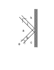
Figure 7: Fused boundary $S$ matrix ${\tilde{\bar{R}}}\!\begin{array}[]{l}{\scriptstyle{\ \ j\ k}}\\ {\scriptstyle{a}}\\ {\scriptstyle{\ \ b\ c}}\end{array}(\theta)$.

satisfies the generalized boundary Yang-Baxter equation

$$\sum_{f\,,g\,,h\,,i}\tilde{\bar{S}}^{\prime a\ h\ c}_{d\ b\ g}(\theta_{1}-\theta_{2})\ \bar{R}\!\begin{array}[]{l}{\ \ \scriptstyle{f}}\\ {\scriptstyle{g}}\\ {\ \ \scriptstyle{c}}\end{array}(\theta_{1})\ {\tilde{\bar{S}}}\!\begin{array}[]{c}{\scriptstyle{g\ e}}\\ {\scriptstyle{h\ i}}\\ {\scriptstyle{d\ f}}\end{array}(\theta_{1}+\theta_{2})\ {\tilde{\bar{R}}}\!\begin{array}[]{l}{\scriptstyle{\ \ j\ k}}\\ {\scriptstyle{e}}\\ {\scriptstyle{\ \ i\ f}}\end{array}(\theta_{2})$$ (B.69)

$$= \sum_{f\,,g\,,h\,,i}{\tilde{\bar{R}}}\!\begin{array}[]{l}{\scriptstyle{\ \ i\ g}}\\ {\scriptstyle{a}}\\ {\scriptstyle{\ \ b\ c}}\end{array}(\theta_{2})\tilde{\bar{S}}^{\prime a\ h\ g}_{d\ i\ f}(\theta_{1}+\theta_{2}+i\pi)\ \bar{R}\!\begin{array}[]{l}{\ \ \scriptstyle{k}}\\ {\scriptstyle{f}}\\ {\ \ \scriptstyle{g}}\end{array}(\theta_{1})\ {\tilde{\bar{S}}}\!\begin{array}[]{c}{\scriptstyle{f\ e}}\\ {\scriptstyle{h\ j}}\\ {\scriptstyle{d\ k}}\end{array}(\theta_{1}-\theta_{2}-i\pi)\,.$$ (B.79)

The shifts in the arguments of the fused bulk $S$ matrices on the RHS should be noted. As an example, for the $NS$ case of the TIM, the nonzero matrix elements of $\tilde{\bar{R}}$ are given by

$${\tilde{\bar{R}}}\!\begin{array}[]{l}{\scriptstyle{\ \ 0\ \sigma}}\\ {\scriptstyle{\sigma}}\\ {\scriptstyle{\ \ 0\ \sigma}}\end{array}(\theta\,,\xi)=\sqrt{2}\cosh{\theta\over 2}\,,\qquad{\tilde{\bar{R}}}\!\begin{array}[]{l}{\scriptstyle{\ \ \sigma\ 0}}\\ {\scriptstyle{0}}\\ {\scriptstyle{\ \ \sigma^{\prime}\ 0}}\end{array}(\theta\,,\xi)={1\over 2\sqrt{2}}(\cosh\theta+\cos\xi)\cosh{\theta\over 2}\,.$$ (B.86)

B.4 Fused transfer matrix

Before attempting to construct the fused transfer matrix, it is instructive to first review the construction of the fundamental transfer matrix. To this end, we set

$$\bar{t}_{a^{\prime}_{1}\ldots a^{\prime}_{N+1}}^{a_{1}\ldots a_{N+1}}(\theta|\theta_{1}\,,\ldots\,,\theta_{N})=\sum_{a^{\prime\prime}_{1}}\bar{R}^{+}\!\begin{array}[]{l}{\scriptstyle{a_{1}}}\\ {\ \ \scriptstyle{a^{\prime\prime}_{1}}}\\ {\scriptstyle{a^{\prime}_{1}}}\end{array}(\theta-i\pi\,,\xi_{+})\ \bar{\cal T}\!\begin{array}[]{c}{\scriptstyle{a_{1}\ldots a_{N+1}}}\\ {\scriptstyle{a^{\prime\prime}_{1}}}\\ {\scriptstyle{a^{\prime}_{1}\ldots a^{\prime}_{N+1}}}\end{array}(\theta|\theta_{1}\,,\ldots\,,\theta_{N})\,,$$ (B.93)

where $\bar{\cal T}$ is defined by

$$\bar{\cal T}\!\begin{array}[]{c}{\scriptstyle{a_{1}\ldots a_{N+1}}}\\ {\scriptstyle{a^{\prime\prime}_{1}}}\\ {\scriptstyle{a^{\prime}_{1}\ldots a^{\prime}_{N+1}}}\end{array}(\theta|\theta_{1}\,,\ldots\,,\theta_{N}) = \sum_{a^{\prime\prime}_{2}\,,\ldots\,,a^{\prime\prime}_{N+1}}\Big{\{}\bar{T}\!\begin{array}[]{c}{\scriptstyle{a^{\prime\prime}_{1}\ldots a^{\prime\prime}_{N+1}}}\\ {\scriptstyle{a^{\prime}_{1}\ldots a^{\prime}_{N+1}}}\end{array}(\theta|\theta_{1}\,,\ldots\,,\theta_{N})\ \bar{R}\!\begin{array}[]{l}{\ \ \scriptstyle{\ a_{N+1}}}\\ {\scriptstyle{a^{\prime\prime}_{N+1}}}\\ {\ \ \scriptstyle{\ a^{\prime}_{N+1}}}\end{array}(\theta\,,\xi_{-})$$ (B.102)

$$\times \hat{\bar{T}}\!\begin{array}[]{c}{\scriptstyle{a_{1}\ldots a_{N+1}}}\\ {\scriptstyle{a^{\prime\prime}_{1}\ldots a^{\prime\prime}_{N+1}}}\end{array}(\theta|\theta_{1}\,,\ldots\,,\theta_{N})\Big{\}}\,,$$ (B.105)

and the monodromy matrices $\bar{T}$ and $\hat{\bar{T}}$ are given by

$$\bar{T}\!\begin{array}[]{c}{\scriptstyle{a_{1}\ldots a_{N+1}}}\\ {\scriptstyle{a^{\prime}_{1}\ldots a^{\prime}_{N+1}}}\end{array}(\theta|\theta_{1}\,,\ldots\,,\theta_{N}) = S_{a_{1}\ a^{\prime}_{2}}^{a^{\prime}_{1}\ a_{2}}(\theta-\theta_{1})\ldots S_{a_{N}\ a^{\prime}_{N+1}}^{a^{\prime}_{N}\ a_{N+1}}(\theta-\theta_{N})\,,$$ (B.108)

$$\hat{\bar{T}}\!\begin{array}[]{c}{\scriptstyle{a_{1}\ldots a_{N+1}}}\\ {\scriptstyle{a^{\prime}_{1}\ldots a^{\prime}_{N+1}}}\end{array}(\theta|\theta_{1}\,,\ldots\,,\theta_{N}) = S_{a^{\prime}_{N}\ a_{N+1}}^{a^{\prime}_{N+1}\ a_{N}}(\theta+\theta_{N})\ldots S_{a^{\prime}_{1}\ a_{2}}^{a^{\prime}_{2}\ a_{1}}(\theta+\theta_{1})\,.$$ (B.111)

The boundary matrix $\bar{R}$ in (B.105) is assumed to obey the boundary Yang-Baxter equation (A.35), which implies that $\bar{\cal T}$ obeys

$$\sum_{c_{1}\,,b_{1}\,,\ldots\,,b_{N+1}}\bar{S}^{e\ c_{1}}_{a^{\prime\prime}_{1}\ a^{\prime}_{1}}(\theta_{1}-\theta_{2})\ \bar{\cal T}\!\begin{array}[]{c}{\scriptstyle{b_{1}\ldots b_{N+1}}}\\ {\scriptstyle{c_{1}}}\\ {\scriptstyle{a^{\prime}_{1}\ldots a^{\prime}_{N+1}}}\end{array}(\theta_{1})\ \bar{S}^{c_{1}\ d_{1}}_{a^{\prime\prime}_{1}\ b_{1}}(\theta_{1}+\theta_{2})\ \bar{\cal T}\!\begin{array}[]{c}{\scriptstyle{a_{1}\ldots a_{N+1}}}\\ {\scriptstyle{d_{1}}}\\ {\scriptstyle{b_{1}\ldots b_{N+1}}}\end{array}(\theta_{2})$$ (B.118)

$$= \sum_{c_{1}\,,b_{1}\,,\ldots\,,b_{N+1}}\bar{\cal T}\!\begin{array}[]{c}{\scriptstyle{b_{1}\ldots b_{N+1}}}\\ {\scriptstyle{e}}\\ {\scriptstyle{a^{\prime}_{1}\ldots a^{\prime}_{N+1}}}\end{array}(\theta_{2})\ \bar{S}^{e\ c_{1}}_{a^{\prime\prime}_{1}\ b_{1}}(\theta_{1}+\theta_{2})\ \bar{\cal T}\!\begin{array}[]{c}{\scriptstyle{a_{1}\ldots a_{N+1}}}\\ {\scriptstyle{c_{1}}}\\ {\scriptstyle{b_{1}\ldots b_{N+1}}}\end{array}(\theta_{1})\ \bar{S}^{c_{1}\ d_{1}}_{a^{\prime\prime}_{1}\ a_{1}}(\theta_{1}-\theta_{2})\,.$$ (B.125)

However, the matrix $\bar{R}^{+}$ in (B.93) is not yet specified. Indeed, following Sklyanin [24], the requirement that the transfer matrix obey the commutativity property (3.34) determines the relation which $\bar{R}^{+}$ should satisfy. In this way, we find (using also the properties (A.1)-(A.3)) that

$$\bar{R}^{+}\!\begin{array}[]{l}{\scriptstyle{c}}\\ {\ \ \scriptstyle{a}}\\ {\scriptstyle{b}}\end{array}(\theta\,,\xi_{+})=\bar{R}\!\begin{array}[]{l}{\ \ \scriptstyle{c}}\\ {\scriptstyle{a}}\\ {\ \ \scriptstyle{b}}\end{array}(-\theta\,,\xi_{+})\,,$$ (B.132)

where $\bar{R}\!\begin{array}[]{l}{\ \ \scriptstyle{c}}\\ {\scriptstyle{a}}\\ {\ \ \scriptstyle{b}}\end{array}(\theta\,,\xi)$ obeys (A.35). The result (B.93), (B.132) coincides with the expression (3.33) for the (reduced) fundamental open-chain transfer matrix .

We follow a similar strategy to construct the fused transfer matrix $\tilde{\bar{t}}$. We set

$$\tilde{\bar{t}}_{a^{\prime}_{1}\ldots a^{\prime}_{N+1}}^{a_{1}\ldots a_{N+1}}(\theta|\theta_{1}\,,\ldots\,,\theta_{N})=\sum_{a^{\prime\prime}_{1}\,,b^{\prime\prime}_{1}\,,c^{\prime\prime}_{1}}{\tilde{\bar{R}}^{+}}\!\begin{array}[]{r}{\scriptstyle{a_{1}\ c^{\prime\prime}_{1}}}\\ {\scriptstyle{\quad a^{\prime\prime}_{1}}}\\ {\scriptstyle{a^{\prime}_{1}\ b^{\prime\prime}_{1}}}\end{array}(\theta-i\pi\,,\xi_{+})\ \tilde{\bar{\cal T}}\!\begin{array}[]{c}{\scriptstyle{a_{1}\ldots a_{N+1}}}\\ {\scriptstyle{a^{\prime\prime}_{1}\,,b^{\prime\prime}_{1}\,,c^{\prime\prime}_{1}}}\\ {\scriptstyle{a^{\prime}_{1}\ldots a^{\prime}_{N+1}}}\end{array}(\theta|\theta_{1}\,,\ldots\,,\theta_{N})\,,$$ (B.139)

where $\tilde{\bar{\cal T}}$ is defined by

$$\tilde{\bar{\cal T}}\!\begin{array}[]{c}{\scriptstyle{a_{1}\ldots a_{N+1}}}\\ {\scriptstyle{a^{\prime\prime}_{1}\,,b^{\prime\prime}_{1}\,,c^{\prime\prime}_{1}}}\\ {\scriptstyle{a^{\prime}_{1}\ldots a^{\prime}_{N+1}}}\end{array}(\theta|\theta_{1}\,,\ldots\,,\theta_{N})=\sum_{a^{\prime\prime}_{2}\,,\ldots\,,a^{\prime\prime}_{N+1}\,,\atop b^{\prime\prime}_{N+1}\,,c^{\prime\prime}_{N+1}}\Big{\{}\tilde{\bar{T}}\!\begin{array}[]{c}{\scriptstyle{a^{\prime\prime}_{1}\ldots a^{\prime\prime}_{N+1}}}\\ {\scriptstyle{b^{\prime\prime}_{1}\,,b^{\prime\prime}_{N+1}}}\\ {\scriptstyle{a^{\prime}_{1}\ldots a^{\prime}_{N+1}}}\end{array}(\theta|\theta_{1}\,,\ldots\,,\theta_{N})$$ (B.146)

$$\times {\tilde{\bar{R}}}\!\begin{array}[]{l}{\scriptstyle{\ \ \ c^{\prime\prime}_{N+1}\ a_{N+1}}}\\ {\scriptstyle{a^{\prime\prime}_{N+1}}}\\ {\scriptstyle{\ \ \ b^{\prime\prime}_{N+1}\ a^{\prime}_{N+1}}}\end{array}(\theta\,,\xi_{-})\ \tilde{\hat{\bar{T}}}\!\begin{array}[]{c}{\scriptstyle{a_{1}\ldots a_{N+1}}}\\ {\scriptstyle{c^{\prime\prime}_{1}\,,c^{\prime\prime}_{N+1}}}\\ {\scriptstyle{a^{\prime\prime}_{1}\ldots a^{\prime\prime}_{N+1}}}\end{array}(\theta+i\pi|\theta_{1}\,,\ldots\,,\theta_{N})\Big{\}}\,,$$ (B.153)

where the fused monodromy matrices $\tilde{\bar{T}}$ and $\tilde{\hat{\bar{T}}}$ are given by

$$\tilde{\bar{T}}\!\begin{array}[]{c}{\scriptstyle{a_{1}\ldots a_{N+1}}}\\ {\scriptstyle{b_{1}\,,b_{N+1}}}\\ {\scriptstyle{a^{\prime}_{1}\ldots a^{\prime}_{N+1}}}\end{array}(\theta|\theta_{1}\,,\ldots\,,\theta_{N}) = \sum_{b_{2}\,,\ldots\,,b_{N}}{\tilde{\bar{S}}}\!\begin{array}[]{c}{\scriptstyle{a^{\prime}_{1}\ a_{2}}}\\ {\scriptstyle{b_{1}\ b_{2}}}\\ {\scriptstyle{a_{1}\ a^{\prime}_{2}}}\end{array}(\theta-\theta_{1})\ldots{\tilde{\bar{S}}}\!\begin{array}[]{c}{\scriptstyle{a^{\prime}_{N}\ a_{N+1}}}\\ {\scriptstyle{b_{N}\ b_{N+1}}}\\ {\scriptstyle{a_{N}\ a^{\prime}_{N+1}}}\end{array}(\theta-\theta_{N})\,,$$ (B.163)

$$\tilde{\hat{\bar{T}}}\!\begin{array}[]{c}{\scriptstyle{a_{1}\ldots a_{N+1}}}\\ {\scriptstyle{b_{1}\,,b_{N+1}}}\\ {\scriptstyle{a^{\prime}_{1}\ldots a^{\prime}_{N+1}}}\end{array}(\theta|\theta_{1}\,,\ldots\,,\theta_{N}) = \sum_{b_{2}\,,\ldots\,,b_{N}}\tilde{\bar{S}}^{\prime a^{\prime}_{N+1}\ b_{N}\ a_{N+1}}_{a^{\prime}_{N}\ b_{N+1}\ a_{N}}(\theta+\theta_{N})\ldots\tilde{\bar{S}}^{\prime a^{\prime}_{2}\ b_{1}\ a_{2}}_{a^{\prime}_{1}\ b_{2}\ a_{1}}(\theta+\theta_{1})\,.$$ (B.167)

We determine the relation obeyed by $\tilde{\bar{R}}^{+}$ from the requirement that the fused transfer matrix (B.139) commute with the fundamental transfer matrix (B.93), (B.132),

$$\left[t(\theta|\theta_{1}\,,\ldots\,,\theta_{N})\,,\tilde{\bar{t}}(\theta^{\prime}|\theta_{1}\,,\ldots\,,\theta_{N})\right]=0\,.$$ (B.168)

With the help of the relation obeyed by $\tilde{\bar{\cal T}}$

$$\sum_{g\,,h\,,i\,,\atop a^{\prime}_{1}\,,\ldots\,,a^{\prime}_{N+1}}\tilde{\bar{S}}^{\prime a\ h\ a_{1}}_{d\ b\ g}(\theta_{1}-\theta_{2})\ \bar{\cal T}\!\begin{array}[]{c}{\scriptstyle{a^{\prime}_{1}\ldots a^{\prime}_{N+1}}}\\ {\scriptstyle{g}}\\ {\scriptstyle{a_{1}\ldots a_{N+1}}}\end{array}(\theta_{1})\ {\tilde{\bar{S}}}\!\begin{array}[]{c}{\scriptstyle{g\ e}}\\ {\scriptstyle{h\ i}}\\ {\scriptstyle{d\ a^{\prime}_{1}}}\end{array}(\theta_{1}+\theta_{2})\ \tilde{\bar{\cal T}}\!\begin{array}[]{c}{\scriptstyle{b_{1}\ldots b_{N+1}}}\\ {\scriptstyle{e\,,i\,,j}}\\ {\scriptstyle{a^{\prime}_{1}\ldots a^{\prime}_{N+1}}}\end{array}(\theta_{2})$$ (B.178)

$$= \sum_{g\,,h\,,i\,,\atop a^{\prime}_{1}\,,\ldots\,,a^{\prime}_{N+1}}\tilde{\bar{\cal T}}\!\begin{array}[]{c}{\scriptstyle{a^{\prime}_{1}\ldots a^{\prime}_{N+1}}}\\ {\scriptstyle{a\,,b\,,i}}\\ {\scriptstyle{a_{1}\ldots a_{N+1}}}\end{array}(\theta_{2})\ \tilde{\bar{S}}^{\prime a\ h\ a^{\prime}_{1}}_{d\ i\ f}(\theta_{1}+\theta_{2}+i\pi)\ \bar{\cal T}\!\begin{array}[]{c}{\scriptstyle{b_{1}\ldots b_{N+1}}}\\ {\scriptstyle{f}}\\ {\scriptstyle{a^{\prime}_{1}\ldots a^{\prime}_{N+1}}}\end{array}(\theta_{1})\ {\tilde{\bar{S}}}\!\begin{array}[]{c}{\scriptstyle{f\ e}}\\ {\scriptstyle{h\ j}}\\ {\scriptstyle{d\ b_{1}}}\end{array}(\theta_{1}-\theta_{2}-i\pi)\,,$$ (B.188)

we obtain the following equation for $\tilde{\bar{R}}^{+}$

$$\sum_{b\,,d\,,f\,,g}{\tilde{\bar{S}}}\!\begin{array}[]{c}{\scriptstyle{g\ k}}\\ {\scriptstyle{f\ l}}\\ {\scriptstyle{j\ m}}\end{array}(\theta_{2}-\theta_{1})\ \bar{R}^{+}\!\begin{array}[]{l}{\scriptstyle{d}}\\ {\ \ \scriptstyle{g}}\\ {\scriptstyle{m}}\end{array}(\theta_{1}-i\pi\,,\xi_{+})\ \tilde{\bar{S}}^{\prime a\ f\ d}_{j\ b\ g}(-\theta_{1}-\theta_{2}+2i\pi)\ {\tilde{\bar{R}}^{+}}\!\begin{array}[]{r}{\scriptstyle{e\ c}}\\ {\scriptstyle{\quad a}}\\ {\scriptstyle{d\ b}}\end{array}(\theta_{2}-i\pi\,,\xi_{+})$$ (B.199)

$$= \sum_{b\,,d\,,f\,,g}{\tilde{\bar{R}}^{+}}\!\begin{array}[]{r}{\scriptstyle{d\ b}}\\ {\scriptstyle{\quad k}}\\ {\scriptstyle{m\ l}}\end{array}(\theta_{2}-i\pi\,,\xi_{+})\ {\tilde{\bar{S}}}\!\begin{array}[]{c}{\scriptstyle{g\ k}}\\ {\scriptstyle{f\ b}}\\ {\scriptstyle{j\ d}}\end{array}(-\theta_{1}-\theta_{2}+i\pi)\ \bar{R}^{+}\!\begin{array}[]{l}{\scriptstyle{e}}\\ {\ \ \scriptstyle{g}}\\ {\scriptstyle{d}}\end{array}(\theta_{1}-i\pi\,,\xi_{+})\ \tilde{\bar{S}}^{\prime a\ f\ e}_{j\ c\ g}(\theta_{2}-\theta_{1}+i\pi)\ \,.$$ (B.209)

That is, this relation guarantees the commutativity (B.168). This relation is satisfied by

$${\tilde{\bar{R}}^{+}}\!\begin{array}[]{r}{\scriptstyle{k\ j}}\\ {\scriptstyle{\quad a}}\\ {\scriptstyle{c\ b}}\end{array}(\theta-i\pi\,,\xi_{+})=\sum_{d\,,f\,,g}P_{\ \ \ c\ a}^{+\ b\ g}\ \bar{R}\!\begin{array}[]{l}{\ \ \scriptstyle{f}}\\ {\scriptstyle{g}}\\ {\ \ \scriptstyle{c}}\end{array}(i\pi-\theta\,,\xi_{+})\ \bar{S}_{f\ a}^{g\ d}(-2\theta+i\pi)\ \bar{R}\!\begin{array}[]{l}{\ \ \scriptstyle{k}}\\ {\scriptstyle{d}}\\ {\ \ \scriptstyle{f}}\end{array}(-\theta\,,\xi_{+})\ P_{\ \ \ k\ a}^{+\ d\ j}\,.$$ (B.220)

(B.221)

For the $NS$ case of the TIM, the nonzero matrix elements of $\tilde{\bar{R}}^{+}$ are given by

$${\tilde{\bar{R}}^{+}}\!\begin{array}[]{r}{\scriptstyle{\sigma\ 0}}\\ {\scriptstyle{\quad\sigma}}\\ {\scriptstyle{\sigma\ 0}}\end{array}(\theta-i\pi\,,\xi_{+}) = \sqrt{2}\cosh{\theta\over 2}\,,$$ (B.225)

$${\tilde{\bar{R}}^{+}}\!\begin{array}[]{r}{\scriptstyle{0\ \sigma}}\\ {\scriptstyle{\quad 0}}\\ {\scriptstyle{0\ \sigma^{\prime}}}\end{array}(\theta-i\pi\,,\xi_{+}) = {1\over 2\sqrt{2}}(\cosh\theta+\cos\xi_{+})\cosh{\theta\over 2}\,.$$ (B.229)

To summarize, the fused transfer matrix $\tilde{\bar{t}}$ is given by (B.139)-(B.167), where the fused matrices $\tilde{\bar{S}}$, $\tilde{\bar{S}}^{\prime}$, $\tilde{\bar{R}}$ and $\tilde{\bar{R}}^{+}$ are given by (B.11), (B.33), (B.59) and (B.221), respectively. For the $NS$ case of the TIM, the nonzero matrix elements of the fused transfer matrix are as follows: for $N=$ even,

$$\tilde{\bar{t}}^{\sigma_{1}\ 0\ \sigma_{2}\ \ldots\ 0\ \sigma_{{N\over 2}+1}}_{\sigma_{1}\ 0\ \sigma_{2}\ \ldots\ 0\ \sigma_{{N\over 2}+1}}(\theta|\theta_{1}\,,\ldots\,,\theta_{N}) = 2\cosh^{2}{\theta\over 2}\ (\prod\cosh)\,,$$ (B.230)

$$\tilde{\bar{t}}^{0\ \sigma_{1}\ 0\ \sigma_{2}\ldots\sigma_{N\over 2}\ 0}_{0\ \sigma_{1}\ 0\ \sigma_{2}\ldots\sigma_{N\over 2}\ 0}(\theta|\theta_{1}\,,\ldots\,,\theta_{N}) = {1\over 2}(\cosh\theta+\cos\xi_{+})(\cosh\theta+\cos\xi_{-})\cosh^{2}{\theta\over 2}\ (\prod\cosh)\,;$$

and for $N=$ odd,

$$\tilde{\bar{t}}^{\sigma_{1}\ 0\ \sigma_{2}\ldots\sigma_{N+1\over 2}\ 0}_{\sigma_{1}\ 0\ \sigma_{2}\ldots\sigma_{N+1\over 2}\ 0}(\theta|\theta_{1}\,,\ldots\,,\theta_{N}) = (\cosh\theta+\cos\xi_{-})\cosh^{2}{\theta\over 2}\ (\prod\cosh)\,,$$

$$\tilde{\bar{t}}^{0\ \sigma_{1}\ 0\ldots 0\ \sigma_{N+1\over 2}}_{0\ \sigma_{1}\ 0\ldots 0\ \sigma_{N+1\over 2}}(\theta|\theta_{1}\,,\ldots\,,\theta_{N}) = (\cosh\theta+\cos\xi_{+})\cosh^{2}{\theta\over 2}\ (\prod\cosh)\,,$$ (B.231)

where $(\prod\cosh)$ denotes

$$(\prod\cosh)=\prod_{j=1}^{N}\cosh({1\over 2}(\theta-\theta_{j}))\cosh({1\over 2}(\theta+\theta_{j}))\,.$$ (B.232)

As also discussed in Sec. 4, for a given a transfer matrix (either fundamental $\bar{t}_{a^{\prime}_{1}\ldots a^{\prime}_{N+1}}^{a_{1}\ldots a_{N+1}}$ or fused $\tilde{\bar{t}}_{a^{\prime}_{1}\ldots a^{\prime}_{N+1}}^{a_{1}\ldots a_{N+1}}$), it is convenient to define the following four “sectors”:

$$N=\mbox{ even }-\mbox{ Sector }I : a_{1}\,,a^{\prime}_{1}\,,a_{N+1}\,,a^{\prime}_{N+1}\in\{-1\,,+1\}\,,$$

$$N=\mbox{ even }-\mbox{ Sector }II : a_{1}=a^{\prime}_{1}=a_{N+1}=a^{\prime}_{N+1}=0\,,$$

$$N=\mbox{ odd }-\mbox{ Sector }I : a_{1}\,,a^{\prime}_{1}\in\{-1\,,+1\}\,,\qquad a_{N+1}=a^{\prime}_{N+1}=0\,,$$

$$N=\mbox{ odd }-\mbox{ Sector }II : a_{1}=a^{\prime}_{1}=0\,,\qquad a_{N+1}\,,a^{\prime}_{N+1}\in\{-1\,,+1\}\,.$$ (B.233)

The results (B.230), (B.231) show that, within each sector, the fused transfer matrix is proportional to the adjacency-inclusive identity matrix,

$$\tilde{\bar{t}}^{(\alpha)}(\theta|\theta_{1}\,,\ldots\,,\theta_{N})=g^{(\alpha)}(\theta)\ \mathbb{I}^{(\alpha)}\,,$$ (B.234)

where $\alpha$ runs over the four sectors (B.233), and $g^{(\alpha)}(\theta)$ is given by

$$g^{(\alpha)}(\theta)=\cosh^{2}{\theta\over 2}\prod_{j=1}^{N}\cosh({1\over 2}(\theta-\theta_{j}))\cosh({1\over 2}(\theta+\theta_{j}))\times\left\{\begin{array}[]{c}2\\ {1\over 2}(\cosh\theta+\cos\xi_{+})(\cosh\theta+\cos\xi_{-})\\ (\cosh\theta+\cos\xi_{-})\\ (\cosh\theta+\cos\xi_{+})\end{array}\right.\,,$$ (B.239)

respectively. This is a nontrivial property of the TIM. The supersymmetric sinh-Gordon model enjoys [21] a similar property.

B.5 Fusion formula and quantum determinants

We now derive the important “fusion formula,” from which the TIM inversion identity is obtained. To this end, we first note that $\tilde{\bar{\cal T}}$ (B.153) can be expressed as the fusion of the corresponding fundamental quantities $\bar{\cal T}$ (B.105),

$$\tilde{\bar{\cal T}}\!\begin{array}[]{c}{\scriptstyle{a_{1}\ldots a_{N+1}}}\\ {\scriptstyle{a^{\prime\prime}_{1}\,,b^{\prime\prime}_{1}\,,c^{\prime\prime}_{1}}}\\ {\scriptstyle{a^{\prime}_{1}\ldots a^{\prime}_{N+1}}}\end{array}(\theta|\theta_{1}\,,\ldots\,,\theta_{N}) = \sum_{b_{1}\,,\ldots\,,b_{N+1}\,,\atop f_{1}\,,g_{1}}\Big{\{}P_{\ \ \ a^{\prime\prime}_{1}\ a^{\prime}_{1}}^{+\ b^{\prime\prime}_{1}\ f_{1}}\ \bar{\cal T}\!\begin{array}[]{c}{\scriptstyle{b_{1}\ldots b_{N+1}}}\\ {\scriptstyle{f_{1}}}\\ {\scriptstyle{a^{\prime}_{1}\ldots a^{\prime}_{N+1}}}\end{array}(\theta|\theta_{1}\,,\ldots\,,\theta_{N})\ \bar{S}^{f_{1}\ g_{1}}_{a^{\prime\prime}_{1}\ b_{1}}(2\theta+i\pi)$$ (B.246)

$$\times \bar{\cal T}\!\begin{array}[]{c}{\scriptstyle{a_{1}\ldots a_{N+1}}}\\ {\scriptstyle{g_{1}}}\\ {\scriptstyle{b_{1}\ldots b_{N+1}}}\end{array}(\theta+i\pi|\theta_{1}\,,\ldots\,,\theta_{N})\ P_{\ \ \ a_{1}\ a^{\prime\prime}_{1}}^{+\ g_{1}\ c^{\prime\prime}_{1}}\Big{\}}\,.$$ (B.250)

We next observe that the reduced bulk $S$ matrix obeys

$$\sum_{c}\bar{S}^{a\ b}_{c\ d}(i\pi-2\theta)\ \bar{S}^{a\ b}_{c\ d^{\prime}}(i\pi+2\theta)=\delta_{d\,,d^{\prime}}\zeta_{d}(\theta)A_{a\ d}A_{b\ d}\,,$$ (B.251)

where, for the TIM, the scalar factor $\zeta_{d}(\theta)$ is given by

$$\zeta_{0}(\theta)={1\over 2}\cosh\theta\,,\qquad\zeta_{\pm 1}(\theta)=2\cosh\theta\,.$$ (B.252)

Using also Eqs. (B.221) and (B.125), we obtain the desired fusion formula

$$\tilde{\bar{t}}^{a_{1}\ldots a_{N+1}}_{a^{\prime}_{1}\ldots a^{\prime}_{N+1}}(\theta)=\zeta_{a^{\prime}_{1}}(\theta)\sum_{a^{\prime\prime}_{1}\,,\ldots\,,a^{\prime\prime}_{N}}{\bar{t}}_{a^{\prime}_{1}\ldots a^{\prime}_{N}}^{a^{\prime\prime}_{1}\ldots a^{\prime\prime}_{N}}(\theta)\ {\bar{t}}_{a^{\prime\prime}_{1}\ldots a^{\prime\prime}_{N}}^{a_{1}\ldots a_{N}}(\theta+i\pi)-\bar{\Delta}^{a_{1}\ldots a_{N+1}}_{a^{\prime}_{1}\ldots a^{\prime}_{N+1}}(\theta)\,,$$ (B.253)

where the quantum determinant [40, 26] $\bar{\Delta}(\theta)$ of the transfer matrix is given by

$$\bar{\Delta}^{a_{1}\ldots a_{N+1}}_{a^{\prime}_{1}\ldots a^{\prime}_{N+1}}(\theta) = \sum_{f_{1}\,,\ldots\,,f_{N+1}\,,\atop b\,,c\,,d\,,j\,,k}\Big{\{}\delta(\bar{R}^{+}(\theta\,,\xi_{+}))\!\begin{array}[]{r}{\scriptstyle{a_{1}\ d}}\\ {\scriptstyle{\quad f_{1}}}\\ {\scriptstyle{a^{\prime}_{1}\ c}}\end{array}\ \delta(\bar{R}(\theta\,,\xi_{-}))\!\begin{array}[]{l}{\scriptstyle{\ \ j\ a_{N+1}}}\\ {\scriptstyle{f_{N+1}}}\\ {\scriptstyle{\ \ b\ a^{\prime}_{N+1}}}\end{array}\ P_{\ \ \ f_{1}\ a_{1}}^{-\ k\ \ d}$$ (B.260)

$$\times \delta(\bar{T}(\theta))^{c\ f_{1}\ldots f_{N+1}}_{b\ a^{\prime}_{1}\ldots a^{\prime}_{N+1}}\ \delta(\hat{\bar{T}}(\theta))^{k\ a_{1}\ldots a_{N+1}}_{j\ f_{1}\ldots f_{N+1}}\Big{\}}\,,$$ (B.261)

where the quantum determinants of the monodromy matrices are defined by

$$\delta(\bar{T}(\theta))^{c\ a_{1}\ldots a_{N+1}}_{b\ a^{\prime}_{1}\ldots a^{\prime}_{N+1}} = \sum_{b_{1}\,,\ldots\,,b_{N+1}}P_{\ \ \ a_{1}\ a^{\prime}_{1}}^{-\ c\ \ b_{1}}\ \bar{T}^{b_{1}\ldots b_{N+1}}_{a^{\prime}_{1}\ldots a^{\prime}_{N+1}}(\theta)\ \bar{T}^{a_{1}\ldots a_{N+1}}_{b_{1}\ldots b_{N+1}}(\theta+i\pi)\ P_{\ \ \ a_{N+1}\ a^{\prime}_{N+1}}^{-\ b_{N+1}\ b}\,,$$

$$\delta(\hat{\bar{T}}(\theta))^{c\ a_{1}\ldots a_{N+1}}_{b\ a^{\prime}_{1}\ldots a^{\prime}_{N+1}} = \sum_{b_{1}\,,\ldots\,,b_{N+1}}P_{\ \ \ a^{\prime}_{1}\ a_{1}}^{-\ c\ \ b_{1}}\ \hat{\bar{T}}^{b_{1}\ldots b_{N+1}}_{a^{\prime}_{1}\ldots a^{\prime}_{N+1}}(\theta)\ \hat{\bar{T}}^{a_{1}\ldots a_{N+1}}_{b_{1}\ldots b_{N+1}}(\theta+i\pi)\ P_{\ \ \ a^{\prime}_{N+1}\ a_{N+1}}^{-\ b\ \ \ \ b_{N+1}}\,,$$ (B.262)

and the quantum determinants of the boundary matrices are defined by

$$\delta(\bar{R}(\theta\,,\xi_{-}))\!\begin{array}[]{l}{\scriptstyle{\ \ j\ k}}\\ {\scriptstyle{a}}\\ {\scriptstyle{\ \ b\ c}}\end{array} = \sum_{d\,,f\,,g}P_{\ \ \ a\ c}^{-\ b\ g}\ \bar{R}\!\begin{array}[]{l}{\ \ \scriptstyle{f}}\\ {\scriptstyle{g}}\\ {\ \ \scriptstyle{c}}\end{array}(\theta)\ \bar{S}_{a\ f}^{g\ d}(2\theta+i\pi)\ \bar{R}\!\begin{array}[]{l}{\ \ \scriptstyle{k}}\\ {\scriptstyle{d}}\\ {\ \ \scriptstyle{f}}\end{array}(\theta+i\pi)\ P_{\ \ \ a\ k}^{-\ d\ j}\,,$$ (B.272)

$$\delta(\bar{R}^{+}(\theta\,,\xi_{+}))\!\begin{array}[]{r}{\scriptstyle{k\ j}}\\ {\scriptstyle{\quad a}}\\ {\scriptstyle{c\ b}}\end{array} = \sum_{d\,,f\,,g}P_{\ \ \ c\ a}^{-\ b\ g}\ \bar{R}\!\begin{array}[]{l}{\ \ \scriptstyle{f}}\\ {\scriptstyle{g}}\\ {\ \ \scriptstyle{c}}\end{array}(i\pi-\theta\,,\xi_{+})\ \bar{S}_{f\ a}^{g\ d}(-2\theta+i\pi)\ \bar{R}\!\begin{array}[]{l}{\ \ \scriptstyle{k}}\\ {\scriptstyle{d}}\\ {\ \ \scriptstyle{f}}\end{array}(-\theta\,,\xi_{+})\ P_{\ \ \ k\ a}^{-\ d\ j}\,.$$ (B.282)

We now proceed to evaluate the quantum determinants for the TIM. With the help of the identity

$$\sum_{f\,,g}P_{\ \ \ a\ c}^{-\ b\ g}\ \bar{S}_{g\ d}^{c\ f}(\theta)\ \bar{S}_{a\ f}^{g\ j}(\theta+i\pi)\ P_{\ \ \ j\ d}^{-\ f\ k}=i\sqrt{2}\sinh{\theta\over 2}\ P_{\ \ \ a\ c}^{-\ b\ j}\ P_{\ \ \ j\ d}^{-\ c\ k}\,,$$ (B.283)

we find that the quantum determinants of the monodromy matrices are given by

$$\delta(\bar{T}(\theta))^{c\ a_{1}\ldots a_{N+1}}_{b\ a^{\prime}_{1}\ldots a^{\prime}_{N+1}} = (i\sqrt{2}\sinh{\theta\over 2})^{N}\ P_{\ \ \ a_{1}\ a^{\prime}_{1}}^{-\ c\ \ a_{2}}\ P_{\ \ \ a_{2}\ a^{\prime}_{2}}^{-\ a^{\prime}_{1}\ \ a_{3}}\ldots P_{\ \ \ a_{N+1}\ a^{\prime}_{N+1}}^{-\ a^{\prime}_{N}\ \ \ \ b}\,,$$

$$\delta(\hat{\bar{T}}(\theta))^{c\ a_{1}\ldots a_{N+1}}_{b\ a^{\prime}_{1}\ldots a^{\prime}_{N+1}} = (i\sqrt{2}\sinh{\theta\over 2})^{N}\ P_{\ \ \ a_{1}\ a^{\prime}_{1}}^{-\ c\ \ a^{\prime}_{2}}\ P_{\ \ \ a_{2}\ a^{\prime}_{2}}^{-\ a_{1}\ \ a^{\prime}_{3}}\ldots P_{\ \ \ a_{N+1}\ a^{\prime}_{N+1}}^{-\ a_{N}\ \ \ \ b}\,.$$ (B.284)

Moreover, for the NS case, the quantum determinants of the boundary matrices have the following nonzero matrix elements

$$\delta(\bar{R}(\theta\,,\xi_{-}))\!\begin{array}[]{l}{\scriptstyle{\ \ \ \ 0\ \sigma}}\\ {\scriptstyle{-\sigma}}\\ {\scriptstyle{\ \ \ \ 0\ \sigma}}\end{array} = i\sqrt{2}\sinh{\theta\over 2}\,,$$ (B.288)

$$\delta(\bar{R}(\theta\,,\xi_{-}))\!\begin{array}[]{l}{\scriptstyle{\ \ \sigma\ 0}}\\ {\scriptstyle{0}}\\ {\scriptstyle{\ \ \sigma^{\prime}\ 0}}\end{array} = \pm{i\over 2\sqrt{2}}(\cos\xi_{-}-\cosh\theta)\sinh{\theta\over 2}\,,\qquad\sigma=\pm\sigma^{\prime}\,;$$ (B.292)

and

$$\delta(\bar{R}^{+}(\theta\,,\xi_{+}))\!\begin{array}[]{r}{\scriptstyle{\sigma\ 0}}\\ {\scriptstyle{\quad\ -\sigma}}\\ {\scriptstyle{\sigma\ 0}}\end{array} = -i\sqrt{2}\sinh{\theta\over 2}\,,$$ (B.296)

$$\delta(\bar{R}^{+}(\theta\,,\xi_{+}))\!\begin{array}[]{r}{\scriptstyle{0\ \sigma}}\\ {\scriptstyle{\quad\ 0}}\\ {\scriptstyle{0\ \sigma^{\prime}}}\end{array} = \pm{i\over 2\sqrt{2}}(\cosh\theta-\cos\xi_{+})\sinh{\theta\over 2}\,,\qquad\sigma=\pm\sigma^{\prime}\,.$$ (B.300)

We conclude that the quantum determinant $\bar{\Delta}(\theta)$ for the NS case of the TIM is given by

$$\bar{\Delta}^{(\alpha)}(\theta)=h^{(\alpha)}(\theta)\ \mathbb{I}^{(\alpha)}\,,$$ (B.301)

where $\alpha$ runs over the four sectors (B.233), and $h^{(\alpha)}(\theta)$ is given by

$$h^{(\alpha)}(\theta)=\sinh^{2}{\theta\over 2}\prod_{j=1}^{N}\sinh({1\over 2}(\theta-\theta_{j}))\sinh({1\over 2}(\theta+\theta_{j}))\times\left\{\begin{array}[]{c}2\\ {1\over 2}(\cosh\theta-\cos\xi_{+})(\cosh\theta-\cos\xi_{-})\\ (\cosh\theta-\cos\xi_{-})\\ (\cosh\theta-\cos\xi_{+})\end{array}\right.\,,$$ (B.306)

respectively. Substituting this result, together with the result (B.234), (B.239) into the fusion formula (B.253), we finally arrive at the inversion identity (4.21)-(4.27).

References

- [1] A.B. Zamolodchikov and Al.B. Zamolodchikov, Ann. Phys. 120 (1979) 253; A.B. Zamolodchikov, Sov. Sci. Rev. A2 (1980) 1.
- [2] S. Ghoshal and A.B. Zamolodchikov, Int. J. Mod. Phys. A9 (1994) 3841.
- [3] A.A. Belavin, A.M. Polyakov and A.B. Zamolodchikov, Nucl. Phys. B241 (1984) 333.
- [4] A.B. Zamolodchikov and Al.B. Zamolodchikov, Sov. Sci. Rev. A10 (1989) 269; P. Ginsparg, in Fields, Strings and Critical Phenomena (Elsevier Science Publishers B.V.: 1989); P. Di Francesco, P. Mathieu and D. Sénéchal, Conformal Field Theory (Springer: 1997).
- [5] E. Eichenherr, Phys. Lett. B 151 (1985) 26; M. Bershadsky, V. Knizhnik and M. Teitelman, Phys. Lett. B 151 (1985) 31; D. Friedan, Z. Qiu and S.H. Shenker, Phys. Lett. B 151 (1985) 37; A.B. Zamolodchikov and R.G. Pogosyan, Sov. J. Nucl. Phys. 47 (1988) 929; A.B. Zamolodchikov, Rev. Math. Phys. 1 (1990) 197.
- [6] A.B. Zamolodchikov, JETP Lett. 46 (1987) 160; Adv. Stud. Pure Math. 19 (1989) 641.
- [7] A.B. Zamolodchikov, “Fractional-spin integrals of motion in perturbed conformal field theory,” in Fields, Strings and Quantum Gravity, eds. H. Guo, Z. Qiu and H. Tye, (Gordon and Breach, 1989).
- [8] L. Chim, Int. J. Mod. Phys. A11 (1996) 4491.
- [9] R.I. Nepomechie, “Supersymmetry in the boundary tricritical Ising field theory,” hep-th/0203123.
- [10] R.J. Baxter, Exactly Solved Models in Statistical Mechanics (Academic Press, 1982).
- [11] G.E. Andrews, R.J. Baxter and P.J. Forrester, J. Stat. Phys. 35 (1984) 193.
- [12] C. Ahn, D. Bernard and A. LeClair, Nucl. Phys. B346 (1990) 409.
- [13] C. Ahn and W.M. Koo, Nucl. Phys. B468 (1996) 461; J. Phys. A29 (1996) 5845.
- [14] P. Di Vecchia and S. Ferrara, Nucl. Phys. B130 (1977) 93; J. Hruby, Nucl. Phys. B131 (1977) 275.
- [15] R.I. Nepomechie, Phys. Lett. B509 (2001) 183.
- [16] C.N. Yang and C.P. Yang, J. Math. Phys. 10 (1969) 1115.
- [17] Al.B. Zamolodchikov, Nucl. Phys. B342 (1990) 695.
- [18] Al.B. Zamolodchikov, Nucl. Phys. B358 (1991) 497.
- [19] A. LeClair, G. Mussardo, H. Saleur and S. Skorik, Nucl. Phys. B453 (1995) 581.
- [20] P. Dorey, I. Runkel, R. Tateo and G. Watts, Nucl. Phys. B578 (2000) 85.
- [21] C. Ahn and R.I. Nepomechie, Nucl. Phys. B586 (2000) 611.
- [22] J.L. Cardy, Nucl. Phys. B324 (1989) 581.
- [23] I. Affleck and A.W.W. Ludwig, Phys. Rev. Lett. 67 (1991) 161.
- [24] E.K. Sklyanin, J. Phys. A21 (1988) 2375.
- [25] M. Karowski, Nucl. Phys. B153 (1979) 244; P.P. Kulish, N.Yu. Reshetikhin and E.K. Sklyanin, Lett. Math. Phys. 5 (1981) 393.
- [26] P.P. Kulish and E.K. Sklyanin, Lecture Notes in Physics, Vol. 151, (Springer, 1982) 61.
- [27] L. Mezincescu and R.I. Nepomechie, J. Phys. A25 (1992) 2533.
- [28] E. Date, M. Jimbo, T. Miwa and M. Okado, Lett. Math. Phys. 12 (1986) 209; ibid. 14 (1987) 97; E. Date, M. Jimbo, A. Kuniba, T. Miwa and M. Okado, Nucl. Phys. B290 (1987) 231; Adv. Stud. Pure Math. 16 (1988) 17.
- [29] R.E. Behrend, P.A. Pearce, D.L. O’Brien, J. Stat. Phys. 84 (1996) 1.
- [30] Y.-K. Zhou, Nucl. Phys. B458 (1996) 504.
- [31] F. Lesage, H. Saleur and P. Simonetti, Phys. Lett. B427 (1998) 85.
- [32] I. Affleck, J. Phys. A33 (2000) 6473.
- [33] K. Graham, I. Runkel and G.M.T. Watts, “Renormalisation group flows of boundary theories,” hep-th/0010082.
- [34] G. Feverati, P.A. Pearce and F. Ravanini, Phys. Lett. B534 (2002) 216.
- [35] C.N. Yang, Phys. Rev. Lett. 19 (1967) 1312.
- [36] K. Graham, JHEP 0203 (2002) 028.
- [37] P. Fendley and H. Saleur, Nucl. Phys. B428 (1994) 681.
- [38] M. Grisaru, L. Mezincescu and R.I. Nepomechie, J. Phys. A28 (1995) 1027
- [39] I.V. Cherednik, Theor. Math. Phys. 61 (1984) 977.
- [40] A.G. Izergin and V.E. Korepin, Sov. Phys. Doklady 26 (1981) 653; Nucl. Phys. B205 (1982) 401.
- [41] Al.B. Zamolodchikov, Nucl. Phys. B366 (1991) 122.
- [42] C. Ahn and C. Rim, J. Phys. A32 (1999) 2509.