Rotational Symmetry Breaking in Multi-Matrix Models

Abstract

We consider a class of multi-matrix models with an action which is $O(D)$-invariant, where $D$ is the number of $N\times N$ Hermitian matrices $X_{\mu}$, $\mu=1,\ldots,D$. The action is a function of all the elementary symmetric functions of the matrix $T_{\mu\nu}=Tr(X_{\mu}X_{\nu})/N$. We address the issue whether the $O(D)$ symmetry is spontaneously broken when the size $N$ of the matrices goes to infinity. The phase diagram in the space of the parameters of the model reveals the existence of a critical boundary where the $O(D)$ symmetry is maximally broken.

Dedicated to the memory of João D. Correia

OUTP-02-29P

1 Introduction

Over the last twenty years several multi-matrix models have been considered for the description of a wide range of physical systems, from Statistical Physics to QCD or Quantum Gravity [1, 2, 3, 4]. Although an analytic solution is generally not as easy to achieve as for the single-matrix models, a remarkable number of successes and results have been obtained so far [5]. A general feature of one-matrix models is that they possess an internal global symmetry under some gauge group (e.g. $U(N)$ invariance, where $N$ is the size of the matrix) which determines much of the universal behaviour in the large $N$ limit. This global symmetry is present also in all the most relevant multi-matrix models (Ising model on random lattice [6, 7], the $Q$-state Potts model [8, 9, 10, 11, 12, 13], chain of matrices [14, 15, 16, 17, 18, 19], models for coloring problem [20, 21, 22, 23, 24], vertex models [25, 26, 27, 28, 29], the meander model [30, 31], the $O(n)$-model and some generalizations of it [32, 33, 34, 35, 36, 37, 38, 39, 40, 41], and several others [42, 43, 44, 45, 46, 47, 48, 49, 50]. The list is not complete). However, they do not usually have any further symmetry, except for the $O(n)$ model and its generalizations where the whole set of matrices transform as a $O(n)$ vector. The symmetry of these models is then $U(N)\times O(n)$. Recently a new class of multi-matrix models have been introduced in the framework of Superstring Theory and M-theory and the two main representative are the so-called IKKT-model [51, 52, 53] and the BFSS model [54]. They are proposed to be a non-perturbative definition of type IIB Superstring theory and M-Theory, respectively. In particular the IKKT-model is just one element of a bigger class of matrix models, called Super Yang-Mills Integrals (for an introduction see [55, 56, 57, 58]). The latter are characterized by carrying several (super)symmetries and they are obtained from the complete dimensional reduction of $D$-dimensional $SU(N)$ Super Yang-Mills theories. These integrals also might provide an effective tool for the calculation of the bulk Witten index of a supersymmetric quantum mechanics theory [59, 60, 61, 62, 63].

One consequence of having several symmetries is the existence of flat directions in the action of the model. They are potential sources of divergences when evaluating the integrals. The precise domain of existence of all the Yang-Mills Integrals with and without supersymmetry and for all the gauge groups, has been rigorously determined in [56, 57, 58] (after numerical and analytical studies for small gauge groups in [64, 65, 66, 67, 68], and for large gauge groups in [69, 70, 71, 72, 73, 74, 75]). The existence of such flat directions affects not only the convergence properties of the Super Yang-Mills integrals, but also the behaviour of all the correlation functions and of the spectral density asymptotics. During the last few years it has been claimed that the “rotational” $O(D)$ symmetry (where $D$ is the number of matrices) might be spontaneously broken in the large $N$ limit [76]. This issue has been analyzed in a series of analytical and numerical studies [69, 70, 71, 72, 73, 74, 77, 78, 79, 80, 81] and a possible mechanism for having such a spontaneous symmetry breaking has been proposed in [77, 78, 79].

The basic idea relies on the fact that these integrals contain fermionic degrees of freedom (i.e. matrices with Grassmannian entries) in such a way that the action is a complex number in general. However the action is a real number for lower-dimensional “degenerate” configurations (i.e. when the matrices are linearly dependent). Therefore, when summing over all possible configurations in the partition function the rapid oscillations of the complex action might enhance lower dimensional configurations in the large $N$ limit. In order to shed light on this mechanism, a class of simplified fermionic multi-matrix models having a complex action (and the same $O(D)\times U(N)$ symmetry) has been studied in [79]. In that case, the symmetry breaking actually occurs, and it is shown to be a consequence of the fact that the action is complex. Also, the results in [80] give indications of a spontaneous symmetry breaking in the IKKT-model. However, the actual mechanism for having such a behaviour (if confirmed) remains an open question.

In this paper we address the question of whether a complex action is necessary if there is to be a spontaneous breaking of the $O(D)$ symmetry at large $N$. The action of the Super-Yang Mills Integrals is complex in general but it also has flat directions. These two features have a quite different origin. The former is a consequence of the particular choice of the structure of the spinors together with the signature of the $D$-dimensional “space-time” in consideration. The latter arises because the action is made up of commutators or logarithms of fermionic determinants (or Pfaffians) (which are there ultimately as a consequence of having an highly symmetric theory). Since it happens that along the flat directions the action becomes real, it is not clear whether the spontaneous symmetry breaking is a consequence of the complexity of the action, or its flatness properties. A definite answer to this question would be given by a complete analytic solution of real-action models such as the Super Yang-Mills integral in four dimension, or its bosonic version (at any $D$) in which the fermions are suppressed. However only numerical simulations are available so far. The results of [82] suggest that there is no spontaneous symmetry breaking in the pure bosonic Yang-Mills integral. About the $4D$ Super Yang-Mills integral there has been some dispute [72, 74] whether there is symmetry breaking or not, and about which is the most reliable order parameter to use in that case (for a review see [83, 84]).

We decide then to focus our attention on building-up a multi-matrix model with a real positive semi-definite action made of standard Hermitian matrices (“bosonic”), but which allow a wide class of possible “degenerate” configurations. In this paper, we shall introduce a multi-matrix model sharing the same $O(D)\times U(N)$ symmetries, but with a real positive weights and without any Grassmannian degrees of freedom. This action allows many degenerate configurations and we will find that they can affect the symmetry of the model at large $N$. This fact is an indication that the exact mechanism which could be at the origin of a possible spontaneous symmetry breaking of rotational symmetries in Super Yang-Mills integrals deserves further studies.

The paper is organized as follows: in Section 2 we define our multi-matrix model. It is based on all the elementary symmetric functions of the eigenvalues of the two-point correlation matrix, and it is manifestly $O(D)$ invariant at finite $N$. The model contains a number of coupling constants which controls the rôle of the various elementary symmetric functions and the interaction among them. We study the behaviour of the model in the space of such parameters. In particular we solve the model in the simple and illuminating case where only two basic elementary symmetric functions are involved, i.e. the trace and the determinant. This case is simple enough for carrying explicit calculations at large $N$ by means of a saddle-point method. In Section 3 we consider the more general case where all the elementary symmetric functions are present. There we show how the model is stable under such a generalization and that the $O(D)$ symmetry of the system holds everywhere except on a critical boundary where the symmetry is maximally broken. Finally, Section 4 is devoted to our discussions and conclusions. For the sake of completeness, the appendix contains the calculation of a Jacobian we make use in Section 2.

2 The model

Let us consider a set of $N\times N$ Hermitian matrices $\{X_{\mu}\}$, $\mu=1,\ldots,D$. The corresponding two-point correlation matrix

$$T_{\mu\nu}\equiv\frac{1}{N}\mbox{Tr\,}(X_{\mu}X_{\nu})$$ (2.1)

is a $D\times D$ real symmetric positive semi-definite matrix, with eigenvalues $t_{1}\geq\cdots\geq t_{D}\geq 0$. From the definition (2.1) we see that if $X_{\mu}\to X_{\mu}^{\prime}=Q_{\mu\nu}X_{\nu}$ where $Q\in O(D)$, then $T$ transforms as $T^{\prime}=QTQ^{T}$. A straightforward consequence is that all the eigenvalues $t_{\mu}$ of $T$ are $O(D)$ invariant quantities. Moreover, the matrices $\{X_{\mu}\}$ are linearly dependent iff some of the eigenvalues $t_{\mu}$ of the correlation matrix $T_{\mu\nu}$ are identically zero. More precisely, a good indicator of the degree of non-degeneracy of the matrices $\{X_{\mu}\}$ is $r(T)\equiv rank(T)$, i.e. the number of non-zero eigenvalues of the matrix $T$. The most general action which is $O(D)$ invariant and is a function of the variables $t_{\mu}$ only, can be expressed in terms of the elementary symmetric functions $c_{k}$ of the variables $\{t_{\mu}\}$, $k=0,\ldots,D$. We recall here that the $k$-th order elementary symmetric function of the variables $\{t_{\mu}\}$ is defined as the products of $k$ distinct variables $t_{\mu}$

$$c_{k}=\sum_{\mu_{1}<\mu_{2}<\ldots<\mu_{k}}t_{\mu_{1}}t_{\mu_{2}}\ldots t_{\mu_{k}}\quad.$$ (2.2)

(we omit the explicit $t_{\mu}$-dependence of $c_{k}$). It is well known that the $c_{k}$ can be obtained from the expansion of the characteristic polynomial of the matrix $T$

$$C(z)\equiv\det({\mathbb{I}}_{D\times D}+zT)=c_{D}z^{D}+c_{D-1}z^{D-1}+\cdots+c_{0}\,.$$ (2.3)

All the $c_{k}$ are non-negative, as the matrix $T$ is positive semi-definite. In particular one has

$$c_{1}={\rm tr\,}T=\frac{1}{N}\sum_{\mu=1}^{D}\mbox{Tr\,}(X_{\mu}^{2})\,,\quad c_{D}=\det\left(\frac{1}{N}\mbox{Tr\,}X_{\mu}X_{\nu}\right)\,,$$

where we use the symbol “Tr” and “tr” to indicate the trace over $N\times N$ and $D\times D$ matrices, respectively.

The partition function we consider in this paper is

$${\cal Z}[\alpha]=\int\prod_{\mu=1}^{D}\mbox{d}X_{\mu}\,e^{-N\mbox{Tr\,}\sum_{\mu=1}^{D}X_{\mu}^{2}}\prod_{k=1}^{D}\left(c_{k}\right)^{\alpha_{k}N^{2}}\,,$$ (2.4)

where $\alpha_{k}$ are real parameters. Eq. (2.4) is manifestly $O(D)$ invariant. This symmetry is not to be confused with the usual $U(N)$ “internal” symmetry, which still holds for this model. In fact ${\cal Z}[\alpha]$ is invariant under $X_{\mu}\rightarrow UX_{\mu}U^{\dagger}$, for all $\mu$, with $U\in U(N)$. The region of existence of this model as a function of the real parameters $\alpha_{k}$ will be determined later in this Section. Here we just emphasize that the argument of the matrix-integrals is always real and positive semi-definite. Moreover, another feature of eq. (2.4) is the existence of “flat directions”. They correspond to configurations where the matrices $\{X_{\mu}\}$ are linearly dependent, i.e. such that some of the symmetric functions $c_{k}$ are identically zero. The convergence properties of the integral (2.4) for large values of the entries of the matrices are mainly guaranteed by the presence of the Gaussian weight, but not completely. In fact, the flat directions contain non-integrable singularities (with some analogy to the case of the Yang-Mills integrals [56, 57, 58]) when some of the parameters $\alpha_{k}$ are too negative. An exact bound in the space of the parameters $\{\alpha_{k}\}$ for the existence of eq. (2.4) is presented in eq. (3.5). At finite $N$ the average eigenvalues $\langle t_{\mu}\rangle$ of the matrix $T$ are all equal, because of the $O(D)$ invariance of eq. (2.4). However at large $N$ this may no longer be the case, and our aim is to see whether the $O(D)$ rotational symmetry of the model can be spontaneously broken when $N\rightarrow\infty$. In this context, we define also the dimensionality $d$ of a configuration of matrices $\{X_{\mu}\}$ as the number of non-vanishing eigenvalues of the average correlation matrix $\langle T\rangle$. Of course, at finite $N$ one always has $d=D$. A possible way for probing $O(D)$ symmetry breaking is to introduce an explicit symmetry breaking term before taking the large $N$ limit. We do this by modifying the Gaussian weight in eq. (2.4) $e^{-N\sum_{\mu}\mbox{Tr\,}(X_{\mu}^{2})}\to e^{-N\sum_{\mu}\lambda_{\mu}\mbox{Tr\,}(X_{\mu}^{2})}$, where the variables $0<\lambda_{1}<\lambda_{2}<\cdots<\lambda_{D}$ maximally break the $O(D)$ symmetry of the model (in analogy to [79]). After taking the large $N$ limit, we shall remove the symmetry breaking term by taking the limit $\lambda_{\mu}\to 1,\forall\mu$. If $\langle t_{\mu}\rangle\to 0$ for different directions $\mu$ then there is spontaneous symmetry breaking of the $O(D)$ symmetry.

We start with the simple case where $\alpha_{2}=\alpha_{3}=\cdots=\alpha_{D-1}=0$. The partition function reads

$${\cal Z}[\alpha,\Lambda]=\int\prod_{\mu=1}^{D}\mbox{d}X_{\mu}\,e^{-N\mbox{Tr\,}\sum_{\mu=1}^{D}\lambda_{\mu}X_{\mu}^{2}}\left({\rm tr\,}T\right)^{\alpha_{1}N^{2}}\left(\det T\right)^{\alpha_{D}N^{2}}$$ (2.5)

It is convenient to introduce the matrix $\Lambda=\delta_{\mu\nu}\lambda_{\mu}$, so that the partition function can be written as ${\cal Z}[\alpha,\Lambda]=\int\prod_{\mu=1}^{D}\mbox{d}X_{\mu}\,\exp(-N^{2}S_{0})$ where the action is

$$S_{0}[T,\alpha,\Lambda]={\rm tr\,}(\Lambda T)-\alpha_{1}\log{\rm tr\,}T-\alpha_{D}\log\det T\,.$$ (2.6)

The action $S_{0}$ depends on all the matrices $X_{\mu}$ only through the matrix $T$: it is therefore natural to change the integration measure from the multi-matrix variables $\{X_{\mu}\}$ to the single-matrix $\{T_{\mu\nu}\}$. When $N^{2}\geq D$ we have (see the Appendix A for details)

$${\cal Z}[\alpha,\Lambda]={\cal C}_{N,D}\int_{T\geq 0}\mbox{d}T\,e^{-N^{2}S[T,\alpha,\Lambda]+\frac{N^{2}-D-1}{2}\log(\det T)}\,,\quad{\cal C}_{N,D}=\frac{N^{\frac{DN^{2}}{2}}\pi^{\frac{D}{4}(2N^{2}-D+1)}}{2^{D\frac{N(N-1)}{2}}\prod_{k=1}^{D}\Gamma\left(\frac{N^{2}-k+1}{2}\right)}\,,$$ (2.7)

where the integral is over all the $D\times D$ real symmetric positive-definite matrices, the measure is $dT=\prod_{\mu\geq\nu}dT_{\mu\nu}$ and the Jacobian of the transformation is proportional to $\det(T)^{\frac{N^{2}-D-1}{2}}$. The partition function now has the proper form for the study of the large $N$ limit by means of the saddle-point (Laplace) method for the asymptotic expansions of multidimensional integrals. According to this method, the main contribution to the integral comes from a small neighborhood of the critical points, i.e. global minimum points in this case, of the action (we drop $1/N^{2}$ sub-leading terms)

$$S[T,\alpha,\Lambda]\equiv{\rm tr\,}T\Lambda-\alpha_{1}\log{\rm tr\,}T-\tilde{\alpha}_{D}\log\det T\,,$$ (2.8)

where $\tilde{\alpha}_{D}\equiv\alpha_{D}+1/2$. The minima of the function $S$ can be at the boundary of the integration region or at the interior of it. In the latter case the necessary stationarity conditions for having a minimum are (saddle-point equations)

$$\frac{\partial}{\partial_{T_{\mu\geq\nu}}}S[T,\alpha,\Lambda]=\lambda_{\mu}\delta_{\mu\nu}-\alpha_{1}\frac{\delta_{\mu\nu}}{{\rm tr\,}T}-\tilde{\alpha}_{D}(T^{-1})_{\nu\mu}=0\,,$$ (2.9)

for all $1\leq\nu\leq\mu\leq D$. Note that multiplying eq. (2.9) by $T$ and taking the trace gives ${\rm tr\,}(T\Lambda)=\alpha_{1}+D\tilde{\alpha}_{D}$. Since ${\rm tr\,}(T\Lambda)\geq 0$ we have to look for solutions of eq. (2.9) in the region of the parameters plane $\{\alpha_{1},\tilde{\alpha}_{D}\}$

$$\alpha_{1}\geq-D\tilde{\alpha}_{D}\,.$$ (2.10)

The condition (2.10) is actually a bound on the domain of existence of the model at large $N$. In fact as we have already announced, the integral in eq. (2.7) exists only when the parameters $\alpha_{k}$ satisfy suitable constraints, and eq. (2.10) is one of them. Namely, the integrand function in eq. (2.7) does not have singularities in the integration region, except perhaps at the integration boundaries. At large values of the entries of $T$ the integrand function is regular and integrable for any value of $\alpha_{k}$, being bounded by the exponential factor. However, the behaviour close to the origin can give non-integrable singularities. This fact is evident when passing to the eigenvalues $\{t_{\mu}\}$ of $T=OtO^{T}$. It yields

$${\cal Z}[\alpha,\Lambda]\sim\int_{0}^{\infty}\prod_{\mu=1}^{D}\mbox{d}t_{\mu}\left|\Delta(t)\right|\,\int_{O(D)}\mbox{d}O\,e^{-N^{2}{\rm tr\,}OtO^{T}\Lambda}\left(\sum_{\mu=1}^{D}t_{\mu}\right)^{\alpha_{1}N^{2}}\left(\prod_{\mu=1}^{D}t_{\mu}\right)^{\alpha_{D}N^{2}+\frac{N^{2}-D-1}{2}}\,,$$ (2.11)

where $\Delta(t)$ is the Vandermonde determinant $\prod_{\mu<\nu}^{D}(t_{\mu}-t_{\nu})$, $\int_{O(D)}$ is the integral over $D\times D$ orthogonal matrices, with Haar measure $\mbox{d}O$, $t$ is a diagonal matrix with diagonal elements $t_{1},\ldots,t_{D}$ and “$\sim$” means “up to a (irrelevant) proportionality constant”. From eq. (2.11) we see that, first, in order to have an integrable singularity at each of the $(D-1)$-dimensional boundary where only one $t_{\mu}=0$, it has to be

$$\alpha_{D}N^{2}+\frac{N^{2}-D-1}{2}>-1\,.$$ (2.12)

At large $N$ this condition simplifies to $\tilde{\alpha}_{D}=\alpha_{D}+1/2\geq 0$. Secondly, by rewriting the integral in eq. (2.11) from cartesian coordinates into multi-dimensional spherical coordinates, one has that the radial integration exists if and only if

$$(D-1)+\frac{D(D-1)}{2}+N^{2}\alpha_{1}+\left(\frac{N^{2}-D-1}{2}+N^{2}\alpha_{D}\right)D>-1\,.$$ (2.13)

Note that there are no contributions from the integral over the orthogonal group: in fact it is finite and regular in $t$, since it is an integral over a compact domain of an analytic function in its variables. At large $N$ the condition (2.13) is fulfilled by $\alpha_{1}+(\frac{1}{2}+\alpha_{D})D\geq 0$ which is precisely eq. (2.10). In summary, the region of existence of the model at large $N$ is

$${\cal D}\equiv\left\{\{\alpha_{k}\}:\alpha_{1}+D\tilde{\alpha}_{D}\geq 0\;\mathrm{and}\;\tilde{\alpha}_{D}\geq 0\right\}\,,$$ (2.14)

and it is depicted in figure 1. We point out that the model at large $N$ is well-defined and finite also on the boundaries of ${\cal D}$, i.e. ${\cal B}_{1}\equiv\{\tilde{\alpha}_{D}=0,\alpha_{1}>0\}$ and ${\cal B}_{0}\equiv\{\alpha_{1}=-D\tilde{\alpha}_{D},\tilde{\alpha}_{D}\geq 0\}$.

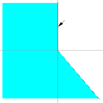
Figure 1: Phase diagram of the model in eq. (2.5). The shaded region is where the partition function is divergent. The wiggle line is the region where the model is one-dimensional. In the remaining region the model maintains the full $O(D)$ dimensionality.

If $\tilde{\alpha}_{D}>0$ then we see immediately that the global minima of $S$ in eq. (2.8) cannot be on the boundary of the integration region. Otherwise the matrix $T$ would have at least a zero eigenvalue, that is $\det T=0$, and there eq. (2.8) gives $S\to+\infty$. Therefore, in this case the critical points must be in the interior of the integration region. Let us then solve eq. (2.9) for $\tilde{\alpha}_{D}>0$. It is straightforward to see that any matrix $T$ which is a solution of eq. (2.9) has to be diagonal. Defining $T=\delta_{\mu\nu}t_{\mu}$ eq. (2.9) reads

$$t_{\mu}=\tilde{\alpha}_{D}\left(\lambda_{\mu}-\frac{\alpha_{1}}{{\rm tr\,}T}\right)^{-1}\,,\quad\mu=1,\ldots D\,.$$ (2.15)

This system of algebraic equations can be solved easily. First, by summing eq. (2.15) over $\mu$ we get an equation for $x\equiv{\rm tr\,}T/\alpha_{1}$,

$$\gamma\equiv\frac{\alpha_{1}}{\tilde{\alpha}_{D}}=\sum_{\mu=1}^{D}\frac{1}{\lambda_{\mu}x-1}\,,\quad x\equiv\frac{{\rm tr\,}T}{\alpha_{1}}\,.$$ (2.16)

For any given real $\gamma$ and $\Lambda$ eq. (2.16) is a rational algebraic equation with $D$ solutions in the variable $x$. All the solutions are real. In fact, by writing the real and imaginary part of $x=x^{\prime}+ix^{\prime\prime}$ and using the fact that $\gamma,\Lambda\in\mathbf{R}$, it yields $x^{\prime\prime}=0$. Among such $D$ real solutions, we have to pick up the ones that make $t_{\mu}\geq 0$ because $T$ has to be a positive semi-definite matrix. From eq. (2.15) we obtain that

$$\left\{\begin{array}[]{lcl}x=\frac{{\rm tr\,}T}{\alpha_{1}}>\frac{1}{\lambda_{1}}&{\rm for}&\alpha_{1}>0\\ &\\ x=\frac{{\rm tr\,}T}{\alpha_{1}}<\frac{1}{\lambda_{D}}&{\rm for}&\alpha_{1}<0\end{array}\right.\,,$$ (2.17)

which is satisfied by only one solution in each case. Namely, for $\alpha_{1}>0$ is $\gamma>0$ and the solution is the largest possible one (the one greater than $1/\lambda_{1}$) whereas for $\alpha_{1}<0$ is $\gamma<0$ and the solution is the one with $x<0$ (see figure 2).

Figure 2: Graphical representation of the r.h.s. of eq. (2.16) as a function of $x=\frac{{\rm tr\,}T}{\alpha_{1}}$. The circles indicate all the solutions. The black circles indicate the acceptable solutions.

For any given point $\{\alpha_{1},\alpha_{D}>0\}$ in the interior of the parameter space ${\cal D}$, if we remove the symmetry breaking terms by taking $\lambda_{\mu}\to 1\,\forall\mu$, then the (unique) solution of eq. (2.16) is $x=1+D/\gamma$, i.e. ${\rm tr\,}T=\alpha_{1}+\tilde{\alpha}_{D}D$. Inserting this value in eq. (2.15) we read that in the large $N$ limit all the eigenvalues are equal to $\langle t_{\mu}\rangle=\alpha_{1}/D+\tilde{\alpha}_{D}$. Hence, we conclude that in the region inside ${\cal D}$ with $\tilde{\alpha}_{D}\neq 0$ the model has a phase with dimensionality $d=D$ and the $O(D)$ symmetry is preserved, as expected. In such a phase, the free energy ${\cal F}=-\frac{1}{N^{2}}\log Z$ reads (with all $\lambda_{\mu}=1$)

$${\cal F}=\left(\alpha_{1}+D\tilde{\alpha}_{D}\right)\left[1-\log\left(\alpha_{1}+D\tilde{\alpha}_{D}\right)\right]+D\tilde{\alpha}_{D}\log D\,.$$ (2.18)

On the boundary ${\cal B}_{0}$ of ${\cal D}$ where $\alpha_{1}=-D\tilde{\alpha}_{D}$ the solution of eqs. (2.15) and (2.16) gives $T=0$. However, it would be wrong to conclude that the dimensionality is $d=0$ there, because actually in the limit $\tilde{\alpha}_{D}\to-\alpha_{1}/D$ one has $T\to 0$ with $d\to D$. That means that there is no spontaneous symmetry breaking on the boundary ${\cal B}_{0}$.

Let us consider now the final case of the boundary ${\cal B}_{1}$ where $\tilde{\alpha}_{D}\to 0^{+}$ first and $\lambda_{\mu}\to 1$ for all $\mu$ afterwards. In such a limit one must consider $\alpha_{1}>0$ in order to stay within the region ${\cal D}$, eq. (2.14), and therefore $\gamma\to+\infty$. According to eq. (2.16) and figure 2, this fact may occur only when $x\to 1/\lambda_{1}$. From eq. (2.15) we have

$$\lim_{\tilde{\alpha}_{D}\to 0^{+}}{\rm tr\,}T=\frac{\alpha_{1}}{\lambda_{1}}\quad\textrm{and }\quad t_{\mu}=\frac{\alpha_{1}}{\lambda_{1}}\delta_{\mu 1}\,.\\$$ (2.19)

In other words, only one eigenvalue of the matrix $T$ is not zero in this limit. Removing the symmetry breaking term by setting $\lambda_{1}\to 1$ leads to a dimensionality $d=1$, actually $\langle t_{\mu}\rangle=\alpha_{1}\delta_{\mu 1}$. That concludes our proof that the model in eq. (2.5) has a maximal spontaneous symmetry breaking of $O(D)$ symmetry whenever $\tilde{\alpha}_{D}\to 0^{+}$.

It is interesting to notice that we could have had considered directly the case $\tilde{\alpha}_{D}=0$ (and not just the limit $\tilde{\alpha}_{D}\to 0^{+}$), because there the model at large $N$ is well-defined. In fact, let $\tilde{\alpha}_{D}=0$ from the very beginning in eq. (2.8). Then, as the $\lambda_{\mu}$’s are all different each other, $S$ cannot have any minima in the interior of the integration domain (in other words, eq. (2.9) do not admit any solution). Hence, the global minimum must be on the boundaries of the integration region, where some $t_{\mu}$ is equal to zero. Analyzing by inspections all the hyperplanes which constitute the integration boundary, one finds that the global minimum is a point on the line $t_{2}=t_{3}=\ldots=t_{D},t_{1}>0$ and it is precisely at $t_{1}=\alpha_{1}/\lambda_{1}$. Substituting this value in eq. (2.8) gives the free energy for the phase ${\cal B}_{1}$

$${\cal F}=\alpha_{1}(1-\log\frac{\alpha_{1}}{\lambda_{1}})\,.$$ (2.20)

This expression (for $\lambda=1$) matches continuously with the free energy in the un-broken phase, eq. (2.18) for $\tilde{\alpha}_{D}\to 0^{+}$. By taking derivatives of the free energies with respect to $\lambda_{\mu}$ we can compute the correlation functions, in particular the average of the eigenvalues, and the susceptibility

$$\langle t_{\mu}\rangle=\left.\frac{\partial{\cal F}}{\partial\lambda_{\mu}}\right|_{\lambda=1}\,,\quad\chi_{\mu\nu}=\left.\frac{\partial^{2}{\cal F}}{\partial\lambda_{\mu}\partial\lambda_{\nu}}\right|_{\lambda=1}=-N^{2}\langle t_{\mu}t_{\nu}\rangle_{conn}\,.$$ (2.21)

In the broken phase ${\cal B}_{1}$, we get from eq. (2.20) and (2.21)

$$\langle t_{\mu}\rangle=\alpha_{1}\delta_{\mu 1}\,,\quad\chi_{\mu\nu}=-\alpha_{1}\delta_{1\mu}\delta_{1\nu}\,.$$ (2.22)

which is of course consistent with eq. (2.19). The computation of the same quantities in the un-broken phase requires the knowledge of an expression of the free energy as a function of $\lambda_{\mu}$ (i.e. eq. (2.18) is not useful for that). A general analytic expression seems not so easy to get since it needs the analytic solutions of the algebraic equation (2.16) in a closed form, which is known to be an impossible task when the degree of the equation is large. However, we can proceed as follows. We already know the pattern of symmetry breaking from eq. (2.19). Hence we can restrict to the case where $\lambda_{1}<\lambda_{2}=\cdots=\lambda_{D}$ without loosing in generality. In this case, eq. (2.16) is a second order algebraic equation which can be solved explicitly. We obtain then the free energy, its first and second derivatives w.r.t. $\lambda_{\mu}$ and in the limit $\lambda_{\mu}\to 1$ they are

$$\langle t_{\mu}\rangle=\frac{\alpha_{1}}{D}+\tilde{\alpha}_{D}\,,\quad\chi_{\mu\nu}=\frac{1}{\tilde{\alpha}_{D}D^{2}}\left(\frac{\alpha_{1}}{D}+\tilde{\alpha}_{D}\right)\times\left\{\begin{array}[]{ll}-\alpha_{1}(D-1)-\tilde{\alpha}_{D}D^{2}&\mathrm{if}\;\mu=\nu\\ \alpha_{1}&\mathrm{if}\;\mu\neq\nu\end{array}\right.\,.$$ (2.23)

Note that the susceptibility is divergent as $\sim 1/\tilde{\alpha}_{D}$ when $\tilde{\alpha}_{D}\to 0$ . The singular behaviour of the susceptibility is again a signal of a criticality at $\tilde{\alpha}_{D}=0$, where the rotational symmetry is actually maximally broken down to one dimension.

3 Generalization

Let us consider now the more general case eq. (2.4) where all the symmetric functions are allowed (and not only $c_{1}$ and $c_{D}$, i.e. the trace and the determinant, respectively). Again introducing the symmetry breaking term $\Lambda_{\mu\nu}=\lambda_{\mu}\delta_{\mu\nu}$, $0<\lambda_{1}<\lambda_{2}<\ldots<\lambda_{D}$, and following the same path of reasoning as in the previous paragraph, we have

$${\cal Z}[\alpha,\Lambda]={\cal C}_{N,D}\int_{T\geq 0}\mbox{d}Te^{-N^{2}S_{N}[T,\alpha,\Lambda]}\,,$$ (3.1)

where the generalized action at finite $N$ is now:

$$S_{N}[T,\alpha,\Lambda]\equiv{\rm tr\,}T\Lambda-\sum_{k=1}^{D}\tilde{\alpha}_{k}\log c_{k}+\frac{D+1}{2N^{2}}\log c_{D}\,,$$ (3.2)

and $\tilde{\alpha}_{k}\equiv\alpha_{k}+\frac{1}{2}\delta_{kD}$. Let us first determine the region of the parameter space $\{\tilde{\alpha}_{k}\}$ where the partition function eq. (3.1) exists. To that aim it is worthwhile to pass to the eigenvalues $t_{1},t_{2},\ldots,t_{D}$ of $T$ in the integral (3.1), as we did in eq. (2.11), thus obtaining a $D$-dimensional integral. The condition which prevents there being a singularity at the point where all the $t_{\mu}$’s are zero is

$$(D-1)+\frac{D(D-1)}{2}+N^{2}\left(\sum_{k=1}^{D}k\tilde{\alpha}_{k}-\frac{D(D+1)}{2N^{2}}\right)>-1$$ (3.3)

as one can see by passing to high-dimensional polar coordinates. More generally, the integrand function does not have singularities on the $p$-dimensional hyperplanes where $D-p$ of the variables $t_{\mu}$’s are zero if and only if

$$(D-p-1)+\frac{(D-p)(D-p-1)}{2}+N^{2}\left(\sum_{k=p+1}^{D}(k-p)\tilde{\alpha}_{k}-\frac{(D-p)(D+1)}{2N^{2}}\right)>-1\,,$$ (3.4)

for $0\leq p\leq D-1$. In the large $N$ limit, the conditions in eq. (3.4) relax to

$$\sum_{k=p+1}^{D}(k-p)\tilde{\alpha}_{k}\geq 0\,,\quad p=0,\ldots,D-1\,.$$ (3.5)

In particular note that $\tilde{\alpha}_{D}\geq 0$. We call ${\cal D}$ the region in the parameter space $\{\tilde{\alpha}_{k}\}$ which is determined by the conditions in eq. (3.5), and from now on we shall consider only values of the parameters $\{\tilde{\alpha}_{k}\}$ which belong to ${\cal D}$. Obviously, this is a natural generalization of the analogous region obtained in eq. (2.14).

The generalized action eq. (3.2) at large $N$ reads

$$S[T,\alpha,\Lambda]\equiv{\rm tr\,}T\Lambda-\sum_{k=1}^{D}\tilde{\alpha}_{k}\log c_{k}\,,$$ (3.6)

and in the same limit the main contribution to the partition function (3.1) comes from the global minima of $S$. Such minima can be in the interior of the integration region or on the boundaries of it. In the former case, the saddle-point equations are

$$\frac{\partial}{\partial_{T_{\mu\geq\nu}}}S[T,\alpha,\Lambda]=\lambda_{\mu}\delta_{\mu\nu}-\sum_{k=1}^{D}\tilde{\alpha}_{k}\frac{1}{c_{k}}\frac{\partial c_{k}}{\partial T_{\mu\geq\nu}}=0\,.$$ (3.7)

Any matrix $T$ which is a solution of eq. (3.7) must be diagonal. In fact, taking the commutator of eq. (3.7) with $T$ yields $[\Lambda,T]=0$ because $T$ commutes with any other function of $T$. Writing the commutator in components reads $(\lambda_{\mu}-\lambda_{\nu})T_{\mu\nu}=0$, i.e. $T$ is diagonal. Thus, letting $T=\delta_{\mu\nu}t_{\mu}$, the saddle-point equations are equivalent to the following system of non-linear algebraic equations

$$\lambda_{\mu}=\sum_{k=1}^{D}\tilde{\alpha}_{k}\frac{1}{c_{k}}\frac{\partial c_{k}}{\partial t_{\mu}}\,,\quad\mu=1,\ldots,D\,.$$ (3.8)

The case where the absolute minima of the action $S$ are instead on the boundary of the integration region can occur only if some parameters $\tilde{\alpha}_{k}$ are identically zero. In fact, if all the parameters $\tilde{\alpha}_{k}$ are different from zero, then the action is positively divergent when at least one $t_{\mu}$ is zero, and thus there cannot be any minima on the boundary.

For the moment, let us restrict the discussion to the case where all the parameters $\tilde{\alpha}_{k}$ are strictly positive. We call ${\cal D}^{+}\subset{\cal D}$ such a region of the parameter space. It is straightforward then to show that in ${\cal D}^{+}$ the system in eq. (3.8) has only one real positive solution (that is a set of $\{t_{1}>0,\ldots t_{D}>0\}$ which fulfills eq. (3.8)), and it is actually the single global minimum of eq. (3.6). In fact, the linear combination ${\rm tr\,}T\Lambda=\sum_{\mu}\lambda_{\mu}t_{\mu}$ and all the elementary symmetric functions $c_{k}$ are multilinear ($k$-affine) functions in the variables $t_{1},\ldots,t_{D}$, as one can directly see from the definition (2.2). As such they are convex functions. Also the function $-\log(x)$ is convex for $x>0$, and therefore the action $S$ in eq. (3.6) is a convex function, being a finite linear combination with positive coefficients of convex functions. Moreover, we show that $S$ is also bounded from below. In fact, we can prove it by using the following inequality

$$\sum_{k=1}^{D}\tilde{\alpha}_{k}\log c_{k}\leq\sum_{k=1}^{D}k\tilde{\alpha}_{k}\log c_{1}\ \,.$$ (3.9)

The proof of the inequality (3.9) is by induction. For $D=1$ it is an identity. Let us suppose that eq. (3.9) is valid for $D-1$. Therefore we have

$$\sum_{k=1}^{D}\tilde{\alpha}_{k}\log c_{k} \leq \sum_{k=1}^{D-1}k\tilde{\alpha}_{k}\log c_{1}+\tilde{\alpha}_{D}\log\left(\frac{c_{D}}{c_{D-1}}\frac{c_{D-1}}{c_{D-2}}\cdots\frac{c_{1}}{c_{0}}\right)$$ (3.10)

$$\leq \sum_{k=1}^{D-1}k\tilde{\alpha}_{k}\log c_{1}+\tilde{\alpha}_{D}\log\left(\frac{c_{1}}{c_{0}}\right)^{D}=\sum_{k=1}^{D}k\tilde{\alpha}_{k}\log c_{1}\,,$$

where we used repeatedly Newton’s inequalities $c_{k}^{2}\geq c_{k-1}c_{k+1}$ for $1\leq k\leq D-1$, in the form $c_{k+1}/c_{k}\leq c_{k}/c_{k-1}$, and the fact that $\tilde{\alpha}_{D}$ is positive in ${\cal D}$. By applying the inequality (3.9) to the effective action eq. (3.6) we get

$$S[T,\alpha,\Lambda]\geq\lambda_{1}c_{1}-\sum_{k=1}^{D}k\tilde{\alpha}_{k}\log c_{1}\,,$$ (3.11)

because ${\rm tr\,}T\Lambda\geq\lambda_{1}\sum_{\mu=1}^{D}t_{\mu}$. Since the function $ax-b\log(x)\geq b(1-\log\frac{b}{a})$ for any $a,b,x$ real and positive, we finally obtain a lower bound for the action

$$S[T,\alpha,\Lambda]\geq A\left(1-\log\frac{A}{\lambda_{1}}\right)\,,$$ (3.12)

where $A\equiv\sum_{k=1}^{D}k\tilde{\alpha}_{k}$ is positive in ${\cal D}$, as follows from eq. (3.5) with $p=0$.

All the above shows that when $\{\tilde{\alpha}_{k}\}\in{\cal D}^{+}$ the action $S$ is continuous, lower bounded and convex in the integration region. From the additional observation that the action is linearly divergent when any $t_{\mu}$ is large and logarithmically divergent when any $t_{\mu}$ is close to zero we conclude that necessarily the action has one and only one global minimum, and it must be in the region $t_{\mu}>0$, $\forall\mu$. We call such a minimum $\bar{t}\equiv\{\bar{t}_{1},\ldots,\bar{t}_{D}\}$, $\bar{t}_{\mu}>0$.

The large $N$ limit of the model is controlled by the behaviour of $\bar{t}$ as a function of $\tilde{\alpha}_{k}$. In the following we enumerate a series of properties of $\bar{t}$. To that aim is worthwhile to recall two useful properties of the elementary symmetric functions [90, 91, 92]. First, the $k$-th order symmetric function $c_{k}$ can always be decomposed as the sum of a $t_{\mu}$-dependent part and a $t_{\mu}$-independent part:

$$c_{k}=t_{\mu}c_{k-1}^{(\mu)}+c_{k}^{(\mu)}\,,$$ (3.13)

where we defined $c_{k}^{(\mu)}\equiv\left.c_{k}\right|_{t_{\mu}=0}$, i.e. the $k$-th elementary symmetric function of $\{t_{1},t_{2},\ldots,t_{D}\}$ omitting $t_{\mu}$. Note that $\partial_{\mu}c_{k}=c_{k-1}^{(\mu)}$. Second, the following equality holds

$$\sum_{\mu=1}^{D}t_{\mu}c_{k}^{(\mu)}=c_{k+1}\,,\quad k=0,\ldots,D-1\,.$$ (3.14)

Let us see now what consequences these properties have on $\bar{t}$.

1. The solution $\bar{t}$ of eq. (3.8) is upper bounded by

   $$\bar{t}_{\mu}\lambda_{\mu}=\sum_{k=1}^{D}\tilde{\alpha}_{k}\frac{\bar{t}_{\mu}c_{k-1}^{(\mu)}}{c_{k}}\leq\sum_{k=1}^{D}\tilde{\alpha}_{k}\,,\quad\forall\mu=1,\ldots,D\,,$$

   because from eq. (3.13) $c_{k}\geq t_{\mu}c_{k-1}^{(\mu)}$.

2. The solution $\bar{t}$ of eq. (3.8) is lower bounded by

   $$\bar{t}_{\mu}=\frac{1}{\lambda_{\mu}}\sum_{k=1}^{D}\tilde{\alpha}_{k}\frac{\bar{t}_{\mu}c_{k-1}^{(\mu)}}{c_{k}}\geq\frac{\tilde{\alpha}_{D}}{\lambda_{\mu}}$$ (3.15)

   because all the terms in the sum are non negative and $\bar{t}_{\mu}c_{D-1}^{\mu}/c_{D}=1$. Therefore $\tilde{\alpha}_{D}$ has to go to zero for $t_{\mu}\to 0$. Note that this condition means that when $\tilde{\alpha}_{D}>0$ there cannot be any spontaneous symmetry breaking at all, since none of the eigenvalues is vanishing. In other words, if there is a phase transition, it must be on the plane $\tilde{\alpha}_{D}=0$.

3. The minima $\bar{t}_{\mu}$ are in general monotonic with respect to $\mu$. Subtracting two equations of the system (3.8) gives

   $$\lambda_{\mu}-\lambda_{\nu}=(\bar{t}_{\nu}-\bar{t}_{\mu})\sum_{k=2}^{D}\tilde{\alpha}_{k}\frac{c_{k-2}^{(\mu,\nu)}}{c_{k}}\,,$$ (3.16)

   and then the ordering $\lambda_{1}<\lambda_{2}<\ldots<\lambda_{D}$ implies $\bar{t}_{1}>\bar{t}_{2}>\ldots>\bar{t}_{D}$. On the other hand , from eq. (3.16) follows also $\bar{t}_{\mu}=\bar{t}_{\nu}$ if and only if $\lambda_{\mu}=\lambda_{\nu}$ i.e. when the symmetry breaking terms are removed. We deduce that at any point of the region ${\cal D}^{+}$, the dimensionality of the system is $d=D$ and the original $O(D)$ symmetry is fully preserved. In this case we obtain (with all $\lambda_{\mu}=1$)

   $$\langle t_{\mu}\rangle=\frac{{\cal A}}{D}\,,\quad{\cal F}={\cal A}\left(1-\log{\cal A}\right)-\sum_{k=1}^{D}\tilde{\alpha}_{k}\log\left[\frac{1}{D^{k}}\left(\begin{array}[]{c}D\\ k\end{array}\right)\right]\,,$$ (3.17)

   with ${\cal A}\equiv\sum_{k=1}^{D}k\tilde{\alpha}_{k}$.

4. Let us consider now the limit $\tilde{\alpha}_{D}\to 0$, while keeping all the other $\tilde{\alpha}_{k<D}$ fixed. In this limit the free energy has to be continuous either there is a symmetry breaking or is not. Its limiting value is given by eq. (3.17) just with $\tilde{\alpha}_{D}$ set to zero everywhere, i.e.

   $${\cal F}_{D}={\cal A}^{\prime}\left(1-\log{\cal A}^{\prime}\right)-\sum_{k=1}^{D-1}\tilde{\alpha}_{k}\log\left[\frac{1}{D^{k}}\left(\begin{array}[]{c}D\\ k\end{array}\right)\right]\,,$$ (3.18)

   with ${\cal A}^{\prime}\equiv\sum_{k=1}^{D-1}k\tilde{\alpha}_{k}$. If there is symmetry breaking then $\bar{t}_{D}\to 0$ (it is the smallest eigenvalue) but no other $\bar{t}_{\mu}$ can go to zero. This is because if there are at least two $\bar{t}_{D-1},\bar{t}_{D}\to 0$ then $c_{D-1}\to 0$ and eq. (3.8) would be inconsistent in the limit (l.h.s. is finite whereas r.h.s. is infinite). The free energy for a $(D-1)$-dimensional broken phase (with $\alpha_{D}=0$) would be:

   $${\cal F}_{D-1}={\cal A}^{\prime}\left(1-\log{\cal A}^{\prime}\right)-\sum_{k=1}^{D-1}\tilde{\alpha}_{k}\log\left[\frac{1}{(D-1)^{k}}\left(\begin{array}[]{c}D-1\\ k\end{array}\right)\right]\,.$$ (3.19)

   In general ${\cal F}_{D}\leq{\cal F}_{D-1}$ with the equality only for $D=2$, or $D>2$ and $\tilde{\alpha}_{2}=\ldots=\tilde{\alpha}_{D-1}=0$. We conclude that there is not spontaneous symmetry breaking when $\tilde{\alpha}_{D}\to 0$, unless for $D=2$, or $D>2$ and $\tilde{\alpha}_{2}=\ldots=\tilde{\alpha}_{D-1}=0$ (which is actually the case we considered in Section 2).

It remains to consider the “wedge” region ${\cal D}/{\cal D}^{+}$ of the phase space, where some of the $\tilde{\alpha}_{k}$ are negative. In this case the action $S$ is no longer a convex function, but it still possible to prove that it has only one global minimum. The proof goes as follows. First of all, $S$ is still lower bounded by the same bound as in eq. (3.12), and it is divergent towards $+\infty$ at the boundaries of the integration region, hence it must have at least one local minimum. Secondly, if $S$ has more than one local minimum then the system of equations (3.8) would have multiple solutions $\bar{t}_{\mu}$ for a set of values of the parameters $\{\tilde{\alpha}_{k}\}$. We know already that when $\{\tilde{\alpha}_{k}\}$ is in ${\cal D}^{+}$ the solution is unique, therefore there must exists a value $\{\tilde{\alpha}_{k}^{\prime}\}$ of the parameters where multiple solutions merge together into the unique one. This implies that the Jacobian $\det\partial\bar{t}(\tilde{\alpha})/\partial\tilde{\alpha}$ has to be singular or zero for that particular value of $\tilde{\alpha}^{\prime}$. However we show now that this is not possible. In fact, let us write the system of equations (3.8) in the more compact form:

$$\lambda=G[t(\tilde{\alpha})]\cdot\tilde{\alpha}$$ (3.20)

where $\lambda=(\lambda_{1},\ldots,\lambda_{D})$, $G_{\mu k}[t]\equiv c_{k-1}^{(\mu)}/c_{k}$ and $\tilde{\alpha}=(\tilde{\alpha}_{1},\ldots,\tilde{\alpha}_{D})$. Equation (3.20) implicitly defines the vector function $t(\tilde{\alpha})$ as a function of $\tilde{\alpha}$. We take the total derivative of the component $\mu$ of eq. (3.20) w.r.t. $\tilde{\alpha}_{i}$ and compute the determinant w.r.t the indexes $\mu,i$ of the obtained expression. One has:

$$\det_{\mu\sigma}\frac{(G[t(\tilde{\alpha})]\cdot\tilde{\alpha})_{\mu}}{\partial t_{\sigma}}\,\,\det_{\sigma i}\frac{\partial t_{\sigma}(\tilde{\alpha})}{\partial\tilde{\alpha}_{i}}=(-1)^{D}\det G[t(\tilde{\alpha})]\,.$$ (3.21)

The first determinant on the l.h.s. of eq. (3.21) is regular and not zero at $\{\tilde{\alpha}^{\prime}\}$, otherwise the eq. (3.8) would not admit any implicit solution but we know it must exist (because the existence of a global minimum). The determinant on the r.h.s. is $\det G=\Delta(t)/\prod_{j=1}^{D}c_{j}$, where $\Delta(t)$ is the Vandermonde determinant. This expression is finite and it zero only if at least two eigenvalues $t_{\mu},t_{\nu}$ are equal each other and then, by means of eq. (3.8), it must be $\lambda_{\mu}=\lambda_{\nu}$ which is not possible by hypothesis. This ends the proof that for any given $\{\tilde{\alpha}_{k}\}$ in the “wedge” regions the action has only one local minimum in the interior of ${\cal D}$, which is then also a global one. The qualitative behaviour of this critical point as a function of the parameters $\tilde{\alpha}$ goes as for the case in ${\cal D}^{+}$. After removing the symmetry breaking terms $\lambda\to 1$, the critical point becomes completely symmetric in its variables and it corresponds to an un-broken phase with $O(D)$ symmetry.

4 Discussion and conclusions

In this paper we have introduced a multi-matrix model where the Hermitian matrices $X_{\mu}$ are interacting through all the elementary symmetric functions of the correlation matrix $T_{\mu\nu}=\mbox{Tr\,}(X_{\mu}X_{\nu})/N$. The main reason for the choice of such a model relies in its interesting features: first, it is manifestly $O(D)\times SU(N)$ invariant, and it allows the study of the issue of the spontaneous symmetry breaking of $O(D)$ symmetry in the large-$N$ limit. Secondly, the action of the model is real, positive definite and it does not contain any Grassmann variables. This is most useful for understanding what we can actually expect from a model without a complex action or rapidly fluctuating potentials. Understanding the effect of a complex action, which is a notorious difficult problem, requires also realizing first what could happen when it is not there. Third, it allows a number of possible “degenerate configurations” in the matrix integration measure and our aim is to understand their rôle in a scenario of spontaneous symmetry breaking. Finally, the model is considerably simple and can be solved analytically, being the interaction among the matrices only through the $O(D)$ “spatial” symmetry and not through the SU($N$) “internal” symmetry (for which there is just a Gaussian weight). We introduced a number of parameters which allows to tune the relative weight of the elementary symmetric functions of the model, and then we focused our attention on the phases of the model in the space of the parameters when $N$ is large. This has been done in two steps: first in Section 2 by studying in full detail a simple case where only two symmetric functions are “switched on” (the trace and the determinant), and afterwards in Section 3 by considering the more general case where all the symmetric functions are present at the same time. In both cases we found that the $O(D)$ symmetry is broken only in the limit $\alpha_{D}\to-1/2$ for $D=2$ or for $D>2$ and $\alpha_{2}=\ldots=\alpha_{D-1}=0$. In these cases the dimensionality of the model collapses down to one dimension.

The qualitative explanation of such a behaviour is simple. Degenerate configurations of the matrices such that the correlation function $T_{\mu\nu}$ has zero eigenvalues, dominate the matrix integration in the large $N$ limit, when the parameters of the model are tuned to a critical value. In particular the parameter $\alpha_{D}$ (which is coupled to the determinant, i.e. the elementary symmetric function most sensitive to “degenerate” configurations) is to be tuned to the critical value $\alpha_{D}=-1/2$ for compensating an analogous “centrifugal” term coming from the Jacobian (see Appendix). At that precise value of $\alpha_{D}=-1/2$, the measure collapse down to one dimensional configurations, quite independently from the presence of other symmetric functions but the trace. This is most evident from the explicit solutions in Sections 2.

The symmetry breaking mechanism of the model in this paper is therefore due to the existence of directions in the matrix integral along which the measure is identically zero. These directions are where the matrices are linearly dependent, with different degree of degeneracy. We learned also that the reality of the action does not seem to stop a generic Hermitian multi-matrix models with $O(D)\times SU(N)$ symmetry from having a spontaneous symmetry breaking of $O(D)$ symmetry when $N$ is large. Of course this does not prevent other real-action multi-matrix models having different patterns of spontaneous symmetry breaking, nor does not say anything about the rôle played by a possible complex term in the action. For all these reasons our findings do not contradict the analysis of [69, 70, 71, 72, 73, 74, 77, 82, 83]. It would be interesting to carry out the analysis contained in this paper to an extended version of the model where the coupling constants $\tilde{\alpha}$ are allowed to be complex numbers. The action would be complex then, and a different pattern of symmetry breaking seems to be possible.
There are extensions of the model where the matrices are not Hermitian but real symmetric or symplectic. The only changes are in slightly different factors in the Jacobian (see Appendix) and they do not affect the large $N$ results of this paper which still would hold in those generalized cases. We conclude by observing that the reason why we can solve this multi-matrix model is that the interaction among the matrices is only through the correlation matrix $T_{\mu\nu}$. For the rest the matrices are actually not interacting with the full internal $SU(N)$ symmetry group, the interaction being just a Gaussian factor. In fact adding a quartic or higher order term to the action (i.e. terms like $\mbox{Tr\,}X_{\mu}X_{\nu}X_{\mu}X_{\nu}$ and $\mbox{Tr\,}X_{\mu}^{2}X_{\nu}^{2}$) would probably change drastically this scenario, but it would also be more difficult to solve, as happens for multi-matrix models like the Yang-Mills integrals.

Acknowledgments:

The authors would like to thank P.Austing, G. Cicuta, T. Jonsson, C.F.Kristjansen, for useful discussions. We also acknowledge J. Nishimura for collaborating at an early stage of this work. The work of G.V. is supported by the EU network on “Discrete Random Geometry”, grant HPRN-CT-1999-00161.

Appendix A Appendix

For the sake of readability, in this Appendix we compute the Jacobian of the transformation in eq. (2.7). It is a well-known result which has appeared several times in the literature, e.g. [85, 86, 87, 88, 89]. The technique we use here is similar to the one in [85]. The integral in eq. (2.4) is of the form

$$I\equiv\int\prod_{\mu=1}^{D}\mbox{d}X_{\mu}\,f(T[X])\,$$ (A.1)

where $f$ is a real function and the $U(N)$-invariant integration measure for each Hermitian matrix is $dX=\prod_{i=1}^{N}dX_{ii}\prod_{i>j}d\mbox{Re}X_{ij}\,d\mbox{Im}X_{ij}$ as usual. First, by inserting the definition eq. (2.1) of the matrix $T$ in the formula (A.1) by means of Dirac $\delta$-functions, we can equivalently write

$$I=\int_{T\geq 0}dT\,f(T)J(T)\,,\qquad J(T)\equiv\int\prod_{\mu=1}^{D}\mbox{d}X_{\mu}\prod_{\alpha\geq\beta}^{D}\delta(T_{\alpha\beta}-\frac{1}{N}\mbox{Tr\,}{X_{\alpha}X_{\beta}})\,.$$

The Jacobian $J(T)$ can be evaluated by using the integral representation of the $\delta$-function

$$J(T) = \int\prod_{\mu=1}^{D}\mbox{d}X_{\mu}\prod_{\alpha\geq\beta}^{D}\int\frac{d\Omega_{\alpha\beta}}{2\pi}e^{i\Omega_{\alpha\beta}(T_{\alpha\beta}-\frac{1}{N}\mbox{Tr\,}{X_{\alpha}X_{\beta}})}$$ (A.2)

$$= \widetilde{{\cal C}}_{N,D}\int d\Omega\,\frac{e^{i\,{\rm tr\,}\Omega T}}{\det(i\Omega)^{N^{2}/2}}\,\qquad\widetilde{{\cal C}}_{N,D}=\frac{N^{\frac{DN^{2}}{2}}\pi^{\frac{D}{2}(N^{2}-D-1)}}{2^{D\left[\frac{N(N-1)}{2}+1\right]}}\,,$$

where in the last equation we performed the Gaussian integral over the matrices $X_{\mu}$, and we collected the elements $\Omega_{\mu\nu}$ into a real symmetric matrix $\Omega$ (giving an additional factor from the measure). The real-symmetric matrix $T$ can be diagonalized by an orthogonal matrix $O$, i.e. $T=OtO^{T}$ where $t$ is a diagonal matrix, with diagonal elements $t_{\mu}\geq 0$. We change the matrix variables $\Omega\to W$ where $W=O^{T}\Omega O$ and we have $dW=d\Omega$, $\det(iW)=\det(i\Omega)$ and

$$J(T) = \widetilde{{\cal C}}_{N,D}\int dW\frac{e^{i{\rm tr\,}Wt}}{\det(iW)^{N^{2}/2}}$$ (A.3)

$$= \widetilde{{\cal C}}_{N,D}(\det T)^{\frac{N^{2}-D-1}{2}}\int dW\frac{e^{i{\rm tr\,}W}}{[\det iW]^{N^{2}/2}}$$

where in the last equation we apply the transformation $W_{\mu\nu}\rightarrow W_{\mu\nu}/\sqrt{t_{\mu}t_{\nu}}$. The remaining $T$-independent integral is completely factorized and it is equal to $2^{D}\pi^{\frac{D(D+3)}{4}}/\prod_{k=1}^{D}\Gamma(\frac{N^{2}-k+1}{2})$. Finally we obtain

$$J(T)=\frac{N^{\frac{DN^{2}}{2}}\pi^{\frac{D}{4}(2N^{2}-D+1)}}{2^{D\frac{N(N-1)}{2}}\prod_{k=1}^{D}\Gamma\left(\frac{N^{2}-k+1}{2}\right)}(\det T)^{\frac{N^{2}-D-1}{2}}\,.$$ (A.4)

The results in this appendix are valid for $N^{2}\geq D$, which is fine for the large $N$ analysis of this paper.

References

- [1] T. Guhr, A. Müller-Groeling and H.A. Weidenmüller, Phys. Rep. 299 (1998) 190 [cond-mat/9707301].
- [2] J.J.M. Verbaarschot and T. Wettig, Ann. Rev. Nucl. Part. Sci. 50, (2000) 343 [hep-ph/0003017].
- [3] P. Di Francesco, P. Ginsparg and J. Zinn-Justin, Phys. Rept. 254 (1995) 1 [hep-th/9306153].
- [4] J. Ambjorn, B. Durhuus and T. Jonsson, Quantum Geometry, Cambridge University Press, 1997.
- [5] V. A. Kazakov, [hep-th/0003064].
- [6] V. A. Kazakov, Phys. Lett. A 119 (1986) 140.
- [7] D. V. Boulatov and V. A. Kazakov, Phys. Lett. B 186 (1987) 379.
- [8] V. Kazakov, Nucl. Phys. B (Proc. Suppl.) 4 (1988) 93.
- [9] I. Kostov, Nucl. Phys. B (Proc. Suppl.) 10A (1989) 295.
- [10] J. M. Daul, [hep-th/9502014].
- [11] P. Zinn-Justin, J. Statist. Phys. 98 (2001) 245 [cond-mat/9903385].
- [12] G. Bonnet, Phys. Lett. B 459 (1999) 575 [hep-th/9904058].
- [13] B. Eynard and G. Bonnet, Phys. Lett. B 463 (1999) 273 [hep-th/9906130].
- [14] I. K. Kostov, Phys. Lett. B 297 (1992) 74 [hep-th/9208053].
- [15] S. Kharchev, . A. Marshakov, A. Mironov, A. Morozov and S. Pakuliak, Nucl. Phys. B 404 (1993) 717 [hep-th/9208044].
- [16] B. Eynard, J. Phys. A 31 (1998) 8081 [cond-mat/9801075].
- [17] B. Eynard and M. L. Mehta, J. Phys. A 31 (1998) 4449 [cond-mat/9710230].
- [18] B. Eynard, Nucl. Phys. B 506 (1997) 633 [cond-mat/9707005].
- [19] S. Chadha, G. Mahoux and M. L. Mehta, J. Phys. A 14 (1981) 579.
- [20] G. M. Cicuta, L. Molinari and E. Montaldi, Phys. Lett. B 306 (1993) 245.
- [21] P. Di Francesco, B. Eynard and E. Guitter, Nucl. Phys. B 516 (1998) 543 [cond-mat/9711050].
- [22] L. Chekhov and C. Kristjansen, Nucl. Phys. B 479 (1996) 683 [hep-th/9605013].
- [23] B. Eynard and C. Kristjansen, Nucl. Phys. B 516 (1998) 529 [cond-mat/9710199].
- [24] I. K. Kostov, [hep-th/0005190].
- [25] P. Zinn-Justin, Europhys. Lett. 50 (2000) 15 [cond-mat/9909250].
- [26] I. K. Kostov, Nucl. Phys. B 575 (2000) 513 [hep-th/9911023].
- [27] D. A. Johnston and P. Plechac, Phys. Lett. A 248 (1998) 37 [hep-lat/9709003].
- [28] D. A. Johnston, Phys. Lett. B 463 (1999) 9 [cond-mat/9812169].
- [29] V. A. Kazakov and P. Zinn-Justin, Nucl. Phys. B 546 (1999) 647 [hep-th/9808043].
- [30] P. Di Francesco, O. Golinelli and E. Guitter, Math. Comput. Model. 26 (1997) 97 [hep-th/9506030].
- [31] Y. Makeenko and I. Chepelev, [hep-th/9601139].
- [32] M. Gaudin and I. Kostov, Phys. Lett. B 220 (1989) 200.
- [33] I. K. Kostov, Mod. Phys. Lett. A 4 (1989) 217.
- [34] I. K. Kostov and M. Staudacher, Nucl. Phys. B 384 (1992) 459 [hep-th/9203030].
- [35] B. Eynard and J. Zinn-Justin, Nucl. Phys. B 386 (1992) 558 [hep-th/9204082].
- [36] B. Eynard and C. Kristjansen, Nucl. Phys. B 455 (1995) 577 [hep-th/9506193].
- [37] B. Eynard and C. Kristjansen, Nucl. Phys. B 466 (1996) 463 [hep-th/9512052].
- [38] B. Durhuus and C. Kristjansen, Nucl. Phys. B 483 (1997) 535 [hep-th/9609008].
- [39] P. Zinn-Justin, Proceedings of the 1999 semester of the MSRI “Random Matrices and their Applications”, MSRI Publications Vol. 40 (2001) [math-ph/9910010].
- [40] P. Zinn-Justin and J.-B. Zuber, Journal of Knot Theory and its Ramifications 9 (2000) 1127–1141 [math-ph/0002020].
- [41] P. Zinn-Justin, [math-ph/0106005].
- [42] M. Engelhardt and S. Levit, Nucl. Phys. B 488 (1997) 735 [hep-th/9609216].
- [43] B. Eynard, E. Guitter and C. Kristjansen, Nucl. Phys. B 528 (1998) 523 [cond-mat/9801281].
- [44] P. Di Francesco, E. Guitter and C. Kristjansen, Nucl. Phys. B 549 (1999) 657 [cond-mat/9902082].
- [45] C. Itzykson and J. B. Zuber, J. Math. Phys. 21 (1980) 411.
- [46] M. L. Mehta, Commun. Math. Phys. 79 (1981) 327.
- [47] M. Staudacher, Phys. Lett. B 305 (1993) 332 [hep-th/9301038].
- [48] M. R. Douglas and M. Li, Phys. Lett. B 348 (1995) 360 [hep-th/9412203].
- [49] J. M. Daul, V. A. Kazakov and I. K. Kostov, Nucl. Phys. B 409 (1993) 311 [hep-th/9303093].
- [50] M. Bertola, B. Eynard and J. Harnad, [nlin.si/0112006].
- [51] N. Ishibashi, H. Kawai, Y. Kitazawa and A. Tsuchiya, Nucl. Phys. B 498, 467 (1997) [hep-th/9612115].
- [52] M. Fukuma, H. Kawai, Y. Kitazawa and A. Tsuchiya, Nucl. Phys. B 510 (1998) 158 [hep-th/9705128].
- [53] H. Aoki, S. Iso, H. Kawai, Y. Kitazawa, A. Tsuchiya and T. Tada, Prog. Theor. Phys. Suppl. 134, 47 (1999) [hep-th/9908038].
- [54] T. Banks, W. Fischler, S.H. Shenker and L. Susskind, Phys. Rev. D 55, 5112 (1997) [hep-th/9610043].
- [55] W. Krauth, J. Plefka and M. Staudacher, Class. Quant. Grav. 17 (2000) 1171 [hep-th/9911170].
- [56] P. Austing and J. F. Wheater, JHEP 0102 (2001) 028 [hep-th/0101071].
- [57] P. Austing and J. F. Wheater, JHEP 0104 (2001) 019 [hep-th/0103159].
- [58] P. Austing, Yang-Mills matrix theory, PhD Thesis, [hep-th/0108128].
- [59] S. Sethi and M. Stern, Commun. Math. Phys. 194 (1998) 675 [hep-th/9705046].
- [60] P. Yi, Nucl. Phys. B 505 (1997) 307 [hep-th/9704098].
- [61] A. V. Smilga, Nucl. Phys. B 266 (1986) 45; Yad. Fiz. 42 (1986) 728.
- [62] A. V. Smilga, Yad. Fiz. 43 (1986) 215.
- [63] M. Staudacher, Phys. Lett. B 488 (2000) 194 [hep-th/0006234].
- [64] W. Krauth, H. Nicolai and M. Staudacher, Phys. Lett. B 431 (1998) 31 [hep-th/9803117].
- [65] W. Krauth and M. Staudacher, Phys. Lett. B 435 (1998) 350 [hep-th/9804199].
- [66] W. Krauth and M. Staudacher, Phys. Lett. B 453 (1999) 253 [hep-th/9902113].
- [67] W. Krauth and M. Staudacher, Nucl. Phys. B 584 (2000) 641 [hep-th/0004076].
- [68] T. Suyama and A. Tsuchiya, Prog. Theor. Phys. 99 (1998) 321[hep-th/9711073].
- [69] J. Ambjorn, K. N. Anagnostopoulos, W. Bietenholz, T. Hotta and J. Nishimura, JHEP 0007 (2000) 013 [hep-th/0003208]
- [70] J. Ambjorn, K. N. Anagnostopoulos, W. Bietenholz, T. Hotta and J. Nishimura, JHEP 0007, (2000) 011 [hep-th/0005147].
- [71] J. Ambjorn, K. N. Anagnostopoulos, W. Bietenholz, T. Hotta and J. Nishimura, Nucl. Phys. Proc. Suppl. 94, 685 (2001) [hep-lat/0009030].
- [72] J. Ambjorn, K. N. Anagnostopoulos, W. Bietenholz, F. Hofheinz and J. Nishimura, Phys. Rev. D 65 (2002) 086001 [hep-th/0104260].
- [73] P. Bialas, Z. Burda, B. Petersson and J. Tabaczek, Nucl. Phys. B 592 (2001) 391 [hep-lat/0007013].
- [74] Z. Burda, B. Petersson and J. Tabaczek, Nucl. Phys. B 602 (2001) 399 [hep-lat/0012001].
- [75] G. W. Moore, N. Nekrasov and S. Shatashvili, Commun. Math. Phys. 209, 77 (2000) [hep-th/9803265].
- [76] H. Aoki, S. Iso, H. Kawai, Y. Kitazawa and T. Tada, Prog. Theor. Phys. 99 (1998) 713 [hep-th/9802085].
-
[77]
J. Nishimura and G. Vernizzi,
JHEP 0004 (2000) 015 [hep-th/0003223];
Phys. Rev. Lett. 85 (2000) 4664 [hep-th/0007022]. - [78] J. Nishimura and F. Sugino, JHEP 0205 (2002) 001 [hep-th/0111102].
- [79] J. Nishimura, Phys. Rev. D 65 (2002) 105012 [hep-th/0108070].
- [80] H. Kawai, S. Kawamoto, T. Kuroki, T. Matsuo and S. Shinohara, [hep-th/0204240].
- [81] J. Nishimura, T. Okubo and F. Sugino, [hep-th/0205253].
- [82] T. Hotta, J. Nishimura and A. Tsuchiya, Nucl. Phys. B 545 (1999) 543 [hep-th/9811220].
- [83] J. Ambjorn, K. N. Anagnostopoulos, W. Bietenholz, F. Hofheinz and J. Nishimura, Nucl. Phys. Proc. Suppl. 106 (2002) 965-967 [hep-lat/0110094].
- [84] J. Ambjorn, Nucl. Phys. Proc. Suppl. 106 (2002) 62 [hep-lat/0201012].
- [85] F. David, B. Duplantier and E. Guitter, Nucl. Phys. B 394 (1993) 555 [hep-th/9211038].
- [86] Y. V. Fyodorov, Nucl. Phys. B 621 (2002) 643, [math-ph/0106006].
- [87] A. E. Ingham, Proc. Camb. Phil. Soc. 29, (1933) 271.
- [88] C. L. Siegel, Ann. Math. 36, (1935) 527.
- [89] G. M. Cicuta, L. Molinari and G. Vernizzi, J. Phys. A 35, (2002) L51, [hep-th/0109160].
- [90] I.G. Macdonald, Symmetric Functions and Hall Polynomials, Oxford University Press, 1998.
- [91] C.P. Niculescu, J. Inequal. Pure and Appl. Math., 1(2) (2000) Art. 17.
- [92] S. Chaturvedi and V. Gupta, J. Phys. A, 33 (2000) L251.