Topology change in General Relativity,
and the black-hole black-string transition

Abstract:

In the presence of compact dimensions massive solutions of General Relativity may take one of several forms including the black-hole and the black-string, the simplest relevant background being $\mathbb{R}^{3+1}\times{\bf S}^{1}$. It is shown how Morse theory places constraints on the qualitative features of the phase diagram, and a minimalistic diagram is suggested which describes a first order transition whose only stable phases are the uniform string and the black-hole. The diagram calls for a topology changing “merger” transition in which the black-hole evolves continuously into an unstable black-string phase. As evidence a local model for the transition is presented in which the cone over ${\bf S}^{2}\times{\bf S}^{2}$ plays a central role. Horizon cusps do not appear as precursors to black hole merger. A generalization to higher dimensions finds that whereas the cone has a tachyon function for $d=5$, its stability depends interestingly on the dimension - it is unstable for $d<10$, and stable for $d>10$.

To my wife,

Dorit.

1 Introduction

In a gravitational background with compact dimensions several phases of black object solutions to General Relativity may exist, some of them having distinct horizon topologies, depending on the relative size of the horizon (say the Schwarzschild radius) and relevant length scales in the compact dimensions. As the mass of the object is varied phase transitions are expected to occur between the various phases. For concreteness, consider the simplest case - $3+1$ extended dimensions and a fifth compact dimension of radius $L$, which is denoted here by the $z$ coordinate. Black objects with Schwarzschild radius much smaller than $L$ are expected to closely resemble a 5d Schwarzschild black hole (BH) with a nearly round ${\bf S}^{3}$ horizon topology, since by the equivalence principle local measurements at the vicinity of the BH should not detect the large finite size of the $z$ axis. Very massive black objects on the other hand, will have a horizon size much larger than $L$ and will be extended over the $z$ axis wrapping it completely. Such objects will have ${\bf S}^{2}\times{\bf S}^{1}$ horizon topology and will be referred to as “black strings”. One type of black string is the 4d Schwarzschild solution with the $z$ coordinate added in as a spectator and it will be called here a “uniform string”, while another type of solution may be $z$ dependent, namely, a “non-uniform string”.

An attempt to build a consistent phase diagram for this system will lead us to expect a novel topology change within classical General Relativity. The transition involves a one parameter family of Ricci-flat metrics which passes through the cone over ${\bf S}^{2}\times{\bf S}^{2}$ (locally). This cone may be deformed in one of two ways much like the conifold transition leading to different topologies. Each deformation keeps one incontractible sphere, and “fills-in” the other, so the transition may be described as an ${\bf S}^{2}$ shrinking to zero size and then a different ${\bf S}^{2}$ growing up. In addition to the similarities with the conifold the differences should be pointed out as well - this transition happens in any dimension higher or equal to 5, and there are no Killing spinors.

Gregory and Laflamme (GL) [1, 2] found that the uniform black string solution develops a perturbative instability at a certain critical radius, which they interpreted as a transition to the black hole. Horowitz and Maeda [5] recently surprised many by arguing that the endpoint of the decay of the string could not be the black hole, definitely not in finite affine parameter, basically because of the “no tear” property of horizons. Later Gubser [6] showed that the transition is actually first order by studying local properties of the Gregory-Laflamme point.

These papers studied the transition in one direction, namely starting with the black string and reducing its mass, which will be denoted here by “string $\to$ BH” (not implying that the end point is necessarily a BH). One may consider also the opposite direction - starting with a 5d BH and increasing its mass - this direction will be denoted by “BH $\to$ string”. Regarding this latter direction, Susskind [3] claimed (based on Matrix M theory, analogy and intuition) that the transition from a black hole to a non-uniform string (different from the GL point) would be analogous to a Gross-Witten transition in 2d gauge theory, a third order transition (a transition so smooth that only the third derivative of the free energy jumps).

The original goal of this research was be to determine the phase diagram for this transition, and especially take the “BH $\to$ string” route and identify the critical point where the black hole develops a perturbative instability, expecting it to be related to the self intersection of the horizon - the merger of the north and south poles across the compact dimension.

The motivations were

• A case study of a rich GR phase diagram.

• A system with a horizon merger, without time dependence, which could be a model (both analytically and numerically) for the heavily studied problem of black hole collision.

  In particular, numerical simulations in 4d show (see the review [7] and references therein) that when two BH’s approach each other a cusp forms on the horizon of each BH facing the other one. Would cusps be present here?

• A test for the controversy raised by [5].

  One would like to determine whether there exists a third non-uniform phase as claimed by [5], or features of Gross-Witten transition as claimed in [3].

• A challenge for a quantum interpretation of a topology change in the horizon.

  In string theory or any other theory of quantum gravity a black hole is a high entropy quantum system (for example, the black-hole D-brane model). The process of black hole merger should translate to increased coupling between the respective quantum systems. It would be interesting to understand the irreversible merger point in the quantum theory together with the continuous evolution of the entropy as the two BH’s approach each other, but it will not be discussed in this work.

• Wide relevance for higher dimensional branes and extra dimensions.

  In string theory branes and particles in low dimension often can be interpreted as some fundamental branes in 10d or 11d, and then the issue arises whether they should be considered localized or smeared over the compact directions, which is exactly the transition studied here. This system shows up in many other contexts in string theory as well.

Other contributions include the realization of the connection between the GL instability and negative specific heat [8, 9], a discussion of the charged non-uniform black string [10], an attempt to use the Petrov classification to derive the metric of the non-uniform string [11], a numerical study of a closely related problem [12] and other recent papers [13, 15, 16, 17, 18, 19, 20].

We start in section 2 by setting up the system and our notation and reviewing a number of central contributions which we summarize by an incomplete phase diagram (figure 3), looking like an archeological finding with missing parts.

In section 3 Morse theory is used (after a short review) to demonstrate important constraints on the phase diagram. I argue why these constraints require a topology change transition and disfavor a stable non-uniform phase. Finally I present the simplest (in my opinion), consistent phase diagram (figure 10).

In order to find evidence for a qualitative picture, more qualitative tools (beyond the Morse index) are sought. In section 4 the topology of the various solutions is analyzed, and it is found that the suggested phase diagram requires a topology change – a continuous path of solutions connecting different topologies. That leads me to seek a local model of the topology change within Ricci-flat metrics. Moreover, I conjecture that the point of topology change is also a phase transition point. In the rest of the section, the topological requirements of the local transition are elaborated.

The expected Ricci-flat solutions are sought for in sections 5, 6 and a final summary and discussion is presented in section 7.

Note added: This paper is the published version of [51]. Only minor phrasing changes were made to improve the text but it was not updated. For updates see the review [52].

2 An incomplete phase diagram

Consider a static (no angular momentum) black object in an $\mathbb{R}^{3+1}\times{\bf S}^{1}$ gravitational background, namely extended $3+1$ space-time with a periodic fifth dimension which will be denoted by the $z$ coordinate. The system is characterized by 3 dimensionful constants: $L$ the size of the extra dimension $z\sim z+L$ , $M$ the (4d) mass of the system measured at infinity of $\mathbb{R}^{3}$, and $G_{5}$ the 5d Newton constant. From these a single dimensionless parameter can be constructed

$$\mu=(G_{5}M)/L^{2},$$ (1)

while the 4d effective Newton constant is given by $G_{4}=G_{5}/L$.

The isometries of these solutions are $SO(3)\times U(1)$, where the $SO(3)$ comes from the spherical symmetry in $\mathbb{R}^{3}$ and the $U(1)$ comes from time independence. The most general metric with these isometries is

$$ds^{2}=-e^{2\,A}dt^{2}+ds^{2}_{(r,z)}+e^{2\,C}d\Omega^{2},$$ (2)

which is a general metric in the $(r,z)$ plane together with two functions on the plane $A=A(r,z),\,C=C(r,z)$. The horizon is a line determined by $e^{2\,A}=0$ and $d\Omega^{2}=d\theta^{2}+\sin^{2}{\theta}\,d\phi^{2}$. In 4d one can choose a coordinate system that is especially adapted to cylindrical symmetry [21], but this works best only in 4d.

At least two phases of solutions can be distinguished - a black string with an ${\bf S}^{2}\times{\bf S}^{1}$ horizon topology and a 5d black hole with an ${\bf S}^{3}$ horizon. The uniform black string (figure 1) is given by the 4d Schwarzschild metric with $z$ added as a spectator coordinate

$$ds^{2}=-(1-r_{4}/r)\,dt^{2}+(1-r_{4}/r)^{-1}\,dr^{2}+dz^{2}+r^{2}\,d\Omega^{2}$$ (3)

where the Schwarzschild radius is $r_{4}=2\,G_{4}\,M$.

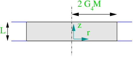
Figure 1: The uniform black-string. $r$ is the radial coordinate in $\mathbb{R}^{3}$.

The small 5d black hole (see figure 2)($r_{5}=\left((8/3\pi)\,G_{5}\,M\right)^{1/2}\ll L$) can be approximated by a combination of two solutions. Denoting the distance from the black hole by $\rho$, for $\rho\ll r_{5}$ it can be approximated by the 5d Schwarzschild BH

$$ds^{2}=-(1-r_{5}^{~{}2}/\rho^{2})\,dt^{2}+(1-r_{5}^{~{}2}/\rho^{2})^{-1}\,d\rho^{2}+\rho^{2}\,d\Omega^{2}_{~{}{\bf S}^{3}}$$ (4)

where $d\Omega^{2}_{~{}{\bf S}^{3}}=d\chi^{2}+\sin^{2}{\chi}\,d\Omega^{2}$. For $\rho\gg r_{5}$ the Newtonian approximation is valid, and the potential is proportional to the Green function

$$V(w)={1\over 4\,r}[\coth(w/2)+\coth(\bar{w}/2)].$$ (5)

where $w:=2\,\pi\,(r+iz)/L$. Indeed close to the source point $w\to 0$, the potential has the expected 5d behavior $V\sim(1/4r)[(2/w)+(2/\bar{w})]=1/(r^{2}+z^{2})$, while for $\mbox{Re}(w)\to\infty$, the 4d behavior is restored $\coth(w)=1+2\exp(-2w),~{}V\sim(1/2r)+O(\exp(-r)$. Presumably a full solution can be built perturbatively in $r_{5}/L$ from these two approximations. Note that following the equipotential surfaces of (5) one encounters already a primitive version of a topology change - close to the source the surface has an ${\bf S}^{3}$ topology, then there is one singular surface with a conic singularity (a cone over ${\bf S}^{2}$) after which the topology of the surfaces changes to ${\bf S}^{2}\times{\bf S}^{1}$.

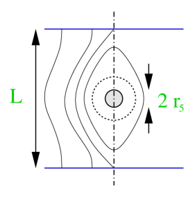
Figure 2: The 5d black-hole with Newtonian equipotential surfaces.

Comparing the areas of the two solutions one finds that for the string the area is

$$A_{string}=4\,\pi\,r_{4}^{~{}2}\,L\sim\mu^{2},$$ (6)

while for the small BH

$$A_{BH}\simeq 2\,\pi^{2}\,r_{5}^{3}\simeq\mu^{3/2}.$$ (7)

Hence, for small $\mu$ the black-hole is preferred, while for larger $\mu$ it is not clear if the black-hole phase exists, but even if it does than if its area would grow as in (7) it would be dominated by the black-string. Therefore a phase transition is expected from the outset.

Let us start by assembling the existing knowledge into an incomplete phase diagram (figure 3). The vertical axis is the parameter $\mu$, while the horizontal axis is an order parameter of non-uniformity $\lambda$. For small $\lambda$ it is defined by $\lambda:=(1-r_{min}/\bar{r})$ where $r_{min},\,\bar{r}$ are the minimum and average respectively of $r=r(z)$, so that $\lambda=0$ exactly when the solution is a uniform string. For large $\lambda$ no precise definition is offered, but consider it to continue to be a measure of non-uniformity even in the black-hole phase.

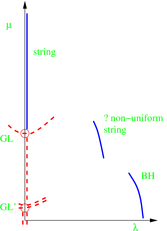
Figure 3: Collecting present data into a phase diagram. $\mu$ is the dimensionless parameter of the problem, and $\lambda$ is an order parameter, a measure of non-uniformity along the $z$ axis. Stable (unstable) phases are denoted by a solid (dashed) lines (double dashed lines denote phases with 2 negative modes). GL denotes the Gregory-Laflamme critical point at $\mu_{GL}$ and GL’ is a copy at $\mu_{GL}/2$.

The horizontal axis is inhabited by the uniform string phase, which changes behavior around the numerically determined Gregory-Laflamme critical point $\mu_{GL}\simeq.070$ corresponding to $(L/r_{4})_{GL}\simeq 7.2$ [1]. We denote the stable (unstable) phase for $\mu>\mu_{GL}$ ($\mu<\mu_{GL}$) by a solid (dashed) line. The black-hole phase, drawn to the left, is known to exist for $\mu\ll 1$ but it is not clear how is evolves for $\mu\sim 1$.

The non-uniform phase (figure 4), argued by Horowitz and Maeda, is depicted for some intermediate values of $\mu$ where the decaying uniform string could end up. However, we must pause and be critical here. Since the predicted solution is not available yet, neither analytically nor numerically ([13, 14]), we stay on the side of caution and mark it by a question mark.

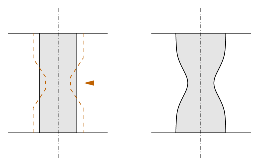
Figure 4: The Gregory-Laflamme unstable mode, and a non-uniform black-string

At the GL critical point the marginally tachyonic mode leads the way to a new phase. A priori this phase could be either stable or unstable (the two possibilities are shown in figure 8). In a beautiful work, initiated by the hope of finding the stable non-uniform phase, Gubser concluded that the emanating phase is actually unstable [6]. This was done by following the solution in a perturbative series near the $GL$ point (to third order in some quantities!). Here again we must be critical, noting that [6] contains a so called “unwanted scheme dependence”, namely the results depend on an unphysical parameter (this dependence looks to me like a missing boundary condition; the local analysis around the GL point is discussed further in the appendix). However, since the results are in some sense only weakly uncertain and since the bottom line agrees so far with unpublished numerical simulations [13, 14], we have some confidence in it.

It should be mentioned that the $GL$ critical point has infinitely many copies at $\mu=\mu_{GL}/n$. These are simply a consequence of the unstable phase of equally spaced $n$ black holes. Since all the phases connected to these copies are duplicates of the basic phases they will be altogether ignored in the rest of the paper. For example, at $\mu=\mu_{GL}/2$ a string with one unstable mode turns into a string with 2 unstable modes, and a new phase with 2 negative modes emanates from the point.

The phase transition, like any other one, can be approached from two different directions, showing possibly different behavior. The two directions will be denoted by “string $\to$ BH” and “BH $\to$ string” but not implying the absence of other phases. So far we discussed only the string $\to$ BH, but this work will concentrate on the opposite one.

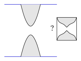
Figure 5: Approaching merger. Do cusps appear?

Regarding the latter, BH $\to$ string direction (figure 5), one should mention the ideas of Susskind [3] on a relation with the Gross-Witten transition in gauge theory [4], stemming from a matrix theory description. In the Gross-Witten transition in 2d large $N$ gauge theories one studies the distribution of eigenvalues of a unitary matrix, $\exp(i\,\theta)$, the matrix being the Wilson loop over an elementary plaquette. The behaviour of the eigenvalues is given precisely by a mechanical model of $N$ point particles moving on a vertical ring (the bottom of the ring is $\theta=0$) in the presence of a uniform gravitational acceleration $g$, a repulsive potential logarithmic at small separations due to the Van-Der-Monde determinant and a temperature $T$ (see figure 6). It is found that one can take a large $N$ limit in such a way that the normalized eigenvalue density distribution approaches a limit $\rho(\theta)$ and a single dimensionless parameter remains, which is essentially $T$. Moreover, whereas the probability density at the top $\rho(\pi)$ never vanishes for finite $N$, it does vanish in the large $N$ limit for small enough $T$. On the other hand, for very large $T$, the distribution becomes uniform $\rho(\theta)=1/(2\,\pi)$. The phase transition occurs at the critical temperature above which $\rho(\pi)>0$ (see figure 6), and it is found to be third order (so smooth that only the third derivative of the free energy jumps).

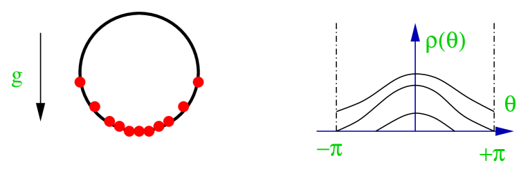
Figure 6: The behavior of the gas of eigenvalues in the Gross-Witten phase transition. The three different density curves are the low temperature “blob” phase analogous to the black-hole, the critical curve, and the high temperature “winding” phase analogous to the black string.

According to [3], the distribution of eigenvalues along the $\theta$ circle is analogous with the mass distribution of the black hole along the $z$ circle, the low $T$ “blob” of eigenvalues is analogous with the black hole phase, and the high $T$ “winding” phase is analogous with the (non-uniform) string. [3] goes on to predict the existence of a Gross-Witten like transition in 4d large $N$ gauge theory, based on the behavior of black holes in a background with a compact 3-torus.

3 Phase diagram - novel constraints

3.1 Euclidean version and Free energy

For Concreteness and convenience, we choose to use the Euclidean signature for the geometries, and to do thermodynamics with the free energy, namely in the canonical ensemble. Since the geometry is time independent we are free to use the Euclidean signature over the Lorentzian. In the Euclidean version “time” is periodic and the circle fiber degenerates over the horizon, so the geometry cannot be continued inside the horizon. Another difference is that Euclidean black hole solutions have a negative mode not present in the Lorentzian version [22] (which is actually the same as the GL mode, and its eigenvalue gives $\mu_{GL}$). Hence we make the convention that the number of negative modes indicated in the phase diagrams is 1 less than that number for the Euclidean version, to conform with the Lorentzian picture. From here on we avoid the Lorentzian signature and any time dependence until the discussion section.

The canonical ensemble offers a direct expression for the free energy $F=F(\beta)$ through the action $I$

$$-\beta\,F=I={1\over 16\,\pi\,G}\int_{\cal M}R+{1\over 8\,\pi\,G}\int_{{\partial}{\cal M}}(K-K_{0})$$ (8)

where the first integral is the bulk contribution of the Ricci scalar and the second is a boundary contribution where $K$ is the trace of the second fundamental form on the boundary, and $K_{0}$ is the same quantity for a reference geometry which is flat $\mathbb{R}^{3}\times{\bf S}^{1}\times{\bf S}^{1}$ in our case. When passing to the canonical ensemble $\beta$ replaces $M$ as a fundamental variable and so $\mu$ is redefined by

$$\mu={\beta\over 8\,\pi\,L}$$ (9)

where the constant factor was determined so that the new and old definitions would coincide for the uniform string. No confusion should arise due to the two definitions of $\mu$ (1,9) since they coincide for the uniform string which was the only place we used $\mu$ so far, and from now only $\mu=\mu(\beta)$ (9) will be used.

In our case, the free energy should be thought to be an even function of $\lambda$. The transformation $\lambda\to-\lambda$ is a symmetry of the action, a remnant of the symmetry of translations in the $z$ direction, which was fixed by the symmetry breaking due to the GL mode.

3.2 Morse theory

Since our goal of understanding the structure of the phase diagram is qualitative rather than quantitative we should seek appropriate qualitative tools. As we follow a curve of solutions, namely an extremum of the free energy, we may encounter a change in stability or a bifurcation point. These transitions and other topological properties of extremal points are the subject of Morse theory, which is our first tool.

We start by reviewing some features of Morse theory. Consider a function $F:\mathbb{R}^{n}\to\mathbb{R}$. For each extremal point $p$ where $\vec{\nabla}F=0$ critical groups and a Morse index are defined. Denoting $F(p)=r,\,F_{y}=\{x:\,F(x)\leq y\}$, the critical groups are given by the local relative homology

$$C_{*}(F,p)=H_{*}(F_{r},F_{r}\backslash\{p\}),$$ (10)

where both sets are intersected with a small enough neighborhood of $p$. The Morse index is the (Euler) index of this homology

$$I_{\mbox{Morse}}(F,p)=\sum_{q}(-)^{q}\,\mbox{dim}(C_{q}(F,p)).$$ (11)

For the generic case of a non-degenerate Hessian ${\partial}_{ij}F(p)$, $n$ the number of its negative eigenvalues, is called “the Morse type”, the critical groups are $C_{n}=\hbox{Z\kern-3.99994ptZ}$ and all the others vanish, and the index is

$$I_{\mbox{Morse}}=(-)^{n}$$ (12)

For a more general extremal point the index is given by considering the function $\vec{\nabla}F/\,|\vec{\nabla}F|$ defined on a small sphere that surrounds $p$ as function from ${\bf S}^{n-1}$ to itself and as such it has a winding number $w$ and one defines

$$I_{\mbox{Morse}}=w(\vec{\nabla}F(p)).$$ (13)

One verifies that the previous definition is indeed a special case of the latter.

One of the basic results is that if we take an arbitrary sphere $S\subset\mathbb{R}^{n}$ with no extremal points then

$$w(\vec{\nabla}F\,(S))=\sum_{p}I_{\mbox{Morse}}(p)$$ (14)

where the sum extends over all the extremal points inside $S$.

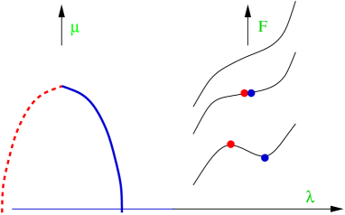
Figure 7: The most generic phase transition - first order with a cubic term. Stable (unstable) phases are denoted by solid (dashed) lines, and an arbitrary number of spectating negative modes $n$ may be added.

As a parameter is changed transitions may occur but the Morse index (and other quantities) stay invariant. The most generic transition is the annihilation (or creation) of a $n,n+1$ type pair. For example in 1d it is the creation of a maximum and minimum pair, and can be modelled by the equation $F(\lambda)=\mu\,\lambda+\lambda^{3}$ (see figure 7). The more general case can be gotten by adding $n$ spectating negative modes.

Out of this primitive vertex one can create more elaborate vertices. The most generic vertex for an even $F$ (figure 8) can be modelled in 1d by $F(\lambda)=\mu\,\lambda^{2}-\lambda^{4}$. It describes a solution with $n=1$ bifurcating into 2 solutions with $n=1$, and one stable solution (one can think of this vertex as the primitive vertex glued to a free line with $n=1$).

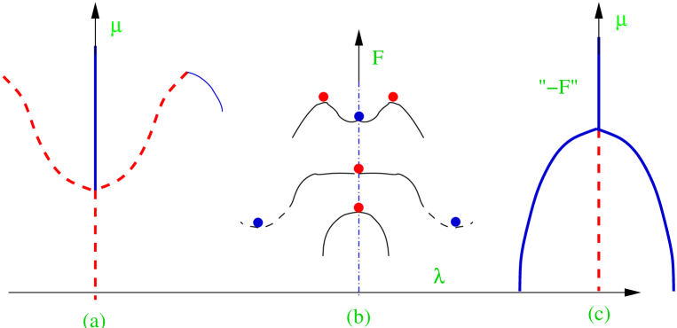
Figure 8: The generic phase transition with even free energy. (a) is the phase diagram corresponding to the free energy $F$ depicted in (b) while (c) is the diagram that corresponds to $-F$ (and $-\mu$).

It can be seen from these examples that it is useful to think about Morse theory as a conservation rule for extremal points under deformations, namely an extremum of type $n$ can only be “annihilated” by a vertex with its “anti-particle”, an extremum of type $n+1$.

3.3 A suggested phase diagram

Let us apply the previous discussion to find consistent ways to complete the phase diagram in figure (3). From the Morse theory “conservation rule” it is now apparent that this diagram has a serious problem – if one assumes that a stable non-uniform string phase exists for $\mu\to 0$ there is an inconsistent non-conservation of phases between $\mu\to 0$ and $\mu\to\infty$. The two “completions” of figure (9) exemplify the problem: diagram (a) has an inconsistent vertex between stable phases, while diagram (b), though consistent, retains the paradox of Horowitz-Maeda [5] intact since the non-uniform phase will have to decay now into a BH.

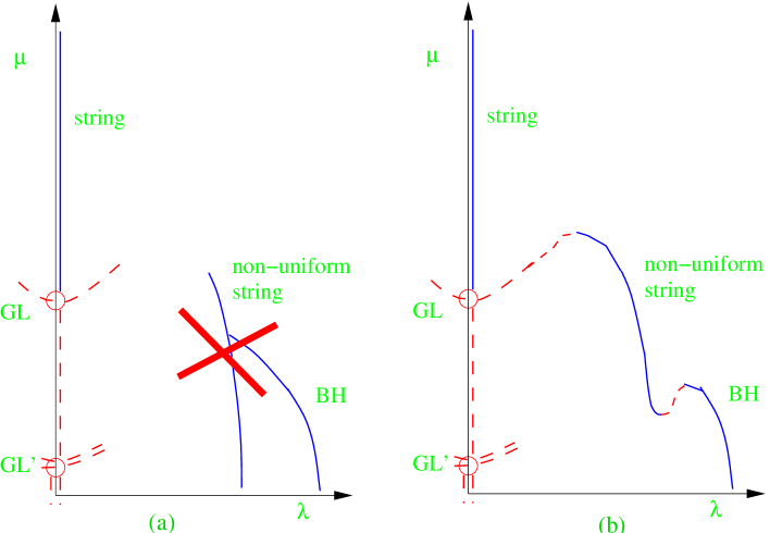
Figure 9: Disfavoured completions of the phase diagram. Diagram (a) is inconsistent as it does not respect the Morse index at the vertex of the black hole and the non-uniform black string. Diagram (b) is consistent but the non-uniform string disappears for small $\mu$ and the paradox of [5] moves to the second transition.

In order to solve the problem there must be either a new phase at the asymptotic regimes $\mu\to 0$ (decompactified 5d) or $\mu\to\infty$ (4d) or a runaway phase (a phase which runs to infinity in field space at finite $\mu$) . Due to these difficulties, and since the stable non-uniform black-string was not constructed yet neither analytically nor numerically, I choose to eliminate it altogether and suggest the following phase diagram (figure 10), which is the simplest option in my opinion. In the suggested phase diagram an unstable non-uniform string emanates from the black string at $\mu_{GL}$ using the even vertex (8) and then simply annihilates the black hole phase, using a generic vertex (7). The latter transition will be called a “merger transition” and its $\mu$ will be denoted by $\mu_{\mbox{merger}}$. Here the point of phase transition is identified with the point of horizon topology change, but a priori these two points are independent. Admittedly, other consistent phase diagrams can be imagined, but this is the simplest one in my opinion. Therefore the challenge now is to seek some confirmation, in which process we will find that changes are due in the neighborhood of the merger transition.

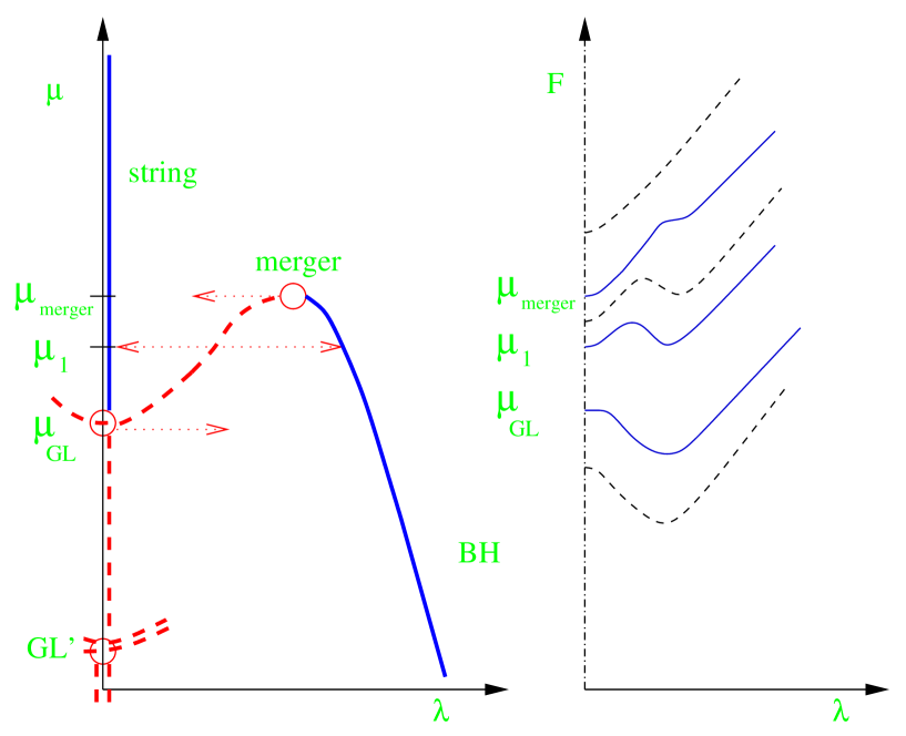
Figure 10: (Left) A suggested phase diagram, which will be refined further in the area of the merger transition. $\mu$ is the dimensionless parameter, and $\lambda$ is an order parameter (measure of non-uniformity). Dotted lines denote transitions - a first order transition at $\mu_{1}$ and tachyonic decay from the two other points. (Right) Curves of the free energy are given for several $\mu$ values, solid lines denoting critical graphs for $F$.

4 Topology - prediction

Let us use another qualitative tool at our disposal namely the topology of the solutions. The black string is contractible to ${\bf S}^{2}\times{\bf S}^{1}$ by contracting the $(r,t)$ plane to a point, hence

$$\mbox{string}\simeq{\bf S}^{2}\times{\bf S}^{1}$$ (15)

where the equivalence denotes homotopic (and homological) equivalence.

The 5d BH is a direct sum of the $\mathbb{R}^{3}\times{\bf S}^{1}_{z}\times{\bf S}^{1}_{t}$ background with the 5d Schwarzschild solution which is topologically a disk bundle over ${\bf S}^{3}$. This topology has the following non-contractible cycles - an ${\bf S}^{1}$ along the $z$ axis, an ${\bf S}^{3}$ along the horizon, and a less obvious ${\bf S}^{2}$ (see figure 11) which is made out of the segment of the $z$ axis connecting the north and south pole, together with the $t$ fiber, which degenerates on the horizon to complete the sphere.

We see that the two solutions have different topologies since the non-contractible 3-cycles have a different topology. This is a much stronger statement than the change in horizon topology. Usually one thinks about the configuration space of GR as being disconnected between different topologies, namely one is given a manifold on which to solve Einstein’s equations together with some boundary conditions, but the topology of the manifold is part of the data, rather than the dynamics. On the other hand we know already about several topology change transitions in 6d or higher such as the flop and the conifold which occur at finite distance in moduli space. Therefore we continue by assuming that such a topology change occurs in our 5d system as well, and seek a local model for it.

Analyzing the topology near the merger transition (see figure 11) we see that the topology of a 4d boundary away from the wall (which hence remains constant during the transition) is ${\bf S}^{2}_{\theta,\phi}\times{\bf S}^{2}_{r,z,t}$ - the line in the $(r,z)$ plane combines with the $t$ circle fiber to give ${\bf S}^{2}_{r,z,t}$ over which the ${\bf S}^{2}_{\theta,\phi}$ is fibered at each point and the fibration can be seen to be trivial due to the decoupled form of the metric 2. In the black-hole phase the ${\bf S}^{2}_{\theta,\phi}$ shrinks completely, while in the string phase the ${\bf S}^{2}_{r,z,t}$ shrinks. So the topology change can be modelled by the “pyramid” familiar from the conifold transition, and the singular solution is the cone over ${\bf S}^{2}\times{\bf S}^{2}$.

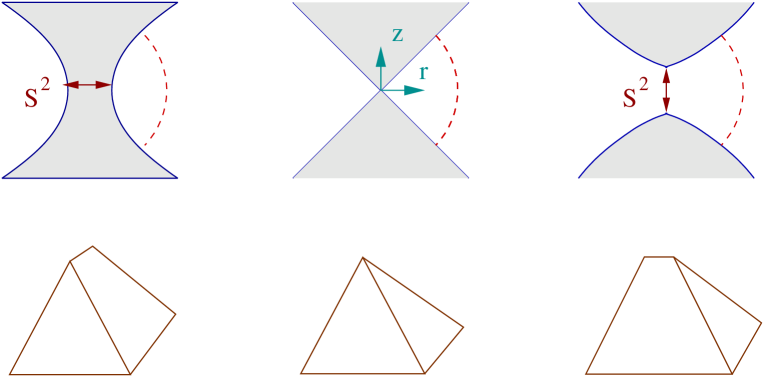
Figure 11: The merger transition. Shaded regions are inside the horizon and the dashed line is the base. The singular configuration is a cone over ${\bf S}^{2}\times{\bf S}^{2}$.

Topologically the transition can be modelled by the equation

$$|\vec{x}|^{2}-\epsilon=|\vec{y}|^{2}$$ (16)

where $\vec{x}\in\mathbb{R}^{3}$ is a 3-vector and , $\vec{y}=(r,t,z)$ combines the $z$ coordinate nicely with $(r,t)$, the origin of $z$ being at the merger point, and the origin of $(r,t)$ on the horizon. For $\epsilon>0$ we have the string, while for $\epsilon<0$ it is the black hole. We view the realization of the transition within the class of Ricci-flat metrics as a challenge for our picture.

5 A local topology change - confirmation

It is required to find Ricci-flat metrics with $SO(3)\times U(1)$ isometry which realize the topology change through the cone over ${\bf S}^{2}\times{\bf S}^{2}$.

5.1 The cone

We start by looking for a Ricci-flat metric for the cone itself, $ds^{2}=d\rho^{2}+\rho^{2}\,ds^{2}_{{\bf S}^{2}\times{\bf S}^{2}}$, which is equivalent to finding an Einstein metric on ${\bf S}^{2}\times{\bf S}^{2}$ with a positive Einstein constant 3 (the unit ${\bf S}^{2}$ has Einstein constant 1). I find that the most general such metric is $3\,ds^{2}_{{\bf S}^{2}\times{\bf S}^{2}}=d\chi^{2}+e^{2c}\,\sin^{2}(\chi)\,d\sigma^{2}+d\theta^{2}+\sin^{2}(\theta)\,d\phi^{2}$, where $c$ is an arbitrary constant which will be set to zero to avoid a unwanted singularity which persists away from the apex. So the geometry is just a product of two round ${\bf S}^{2}$’s with the angle of the cone chosen to assure Ricci flatness

$$ds^{2}=d\rho^{2}+{\rho^{2}\over 3}\left(d\Omega^{2}_{\theta,\phi}+d\Omega^{2}_{\chi,\sigma}\right).$$ (17)

Note that the isometry of the local solution enhances to $SO(3)\times SO(3)$.

Let us verify that this is the only possibility. The $SO(3)\times U(1)$ isometry generates homogeneous 3d orbits $[SO(3)\times U(1)]/U(1)$ which are classified by an integer $k$ giving rise to ${\bf S}^{3}/\hbox{Z\kern-3.99994ptZ}_{k}$ – a circle bundle over ${\bf S}^{2}$ with monopole charge $k$ (with the $\hbox{Z\kern-3.99994ptZ}_{k}$ acting along the Hopf fibration). Then ${\bf S}^{3}/\hbox{Z\kern-3.99994ptZ}_{k}$ must be fibered over an interval (or circle but that would give a trivial fibration and the wrong topology) and “sealed off” at the end-points to make a compact manifold of topology ${\bf S}^{2}\times{\bf S}^{2}$. The possible metrics are $ds^{2}=d\chi^{2}+e^{2\,A}(d\theta^{2}+\sin^{2}(\theta)\,d\phi^{2})+e^{2\,B}(d\sigma-k\,\cos(\theta)\,d\phi)^{2}$. Moreover the discrete $\hbox{Z\kern-3.99994ptZ}_{2}$ isometry of our solution for reflection of the $z$ axis, translates into the functions $A=A(\chi),~{}B=B(\chi)$ being even. If the function $e^{2\,B}$ has zeroes at the end of the interval then we get the Hirzebruch spaces, ${\bf F}_{k}$ - fibrations of ${\bf CP}^{1}$ over ${\bf CP}^{1}$. Therefore the only way to get the product topology ${\bf S}^{2}\times{\bf S}^{2}$ is to start with $k=0$. Then the Einstein equations determine $e^{2\,A}=c_{1},\,e^{2\,B}=c_{2}\,\sin^{2}(\chi)$, as claimed in the previous paragraph.

5.2 The deformed cone

We now proceed to look for Ricci-flat solutions over the deformed cone. A priori I do not know of any obstruction to do that: in 2d the deficit angle of the cone would impose some non-zero curvature (and Ricci) due to Gauss-Bonnet, but that does not apply here.

The ansatz is

$$ds^{2}=d\rho^{2}+e^{2\,a}(d\theta^{2}+\sin^{2}(\theta)\,d\phi^{2})+e^{2\,b}(d\chi^{2}+\sin^{2}(\chi)\,d\sigma^{2})$$ (18)

where $a=a(\rho),~{}b=b(\rho)$ and we retained the enhanced $SU(2)\times SU(2)$ isometries.

The equations are

$$a^{\prime\prime} = e^{-2\,a}-2\,a^{\prime~{}2}-2\,a^{\prime}\,b^{\prime}$$

$$b^{\prime\prime} = e^{-2\,b}-2\,b^{\prime~{}2}-2\,a^{\prime}\,b^{\prime}$$

$$0 = a^{\prime~{}2}+a^{\prime\prime}+b^{\prime~{}2}+b^{\prime\prime}$$ (19)

One verifies that the 3 equations for 2 unknown functions imply a first order constraint

$$0=a^{\prime~{}2}+4\,a^{\prime}\,b^{\prime}+b^{\prime~{}2}-e^{-2\,a}-e^{-2\,b}$$ (20)

which is consistent with the second order equations, and reduces the number of required initial conditions from 4 to 3.

The cone solution corresponds to $a_{0}=b_{0}=\log(\rho)-\log(3)/2$. Let us linearize first the equations around this solution. Denoting

$$\begin{array}[]{lr}a=a_{0}+\alpha&~{}~{}~{}~{}~{}~{}~{}b=b_{0}+\beta\\ \end{array}$$ (21)

we find the linearized equations

$$\alpha^{\prime\prime} = -{6\over\rho^{2}}\,\alpha-{(4+2)\over\rho}\,\alpha^{\prime}-{2\over\rho}\,\beta^{\prime}$$

$$\beta^{\prime\prime} = -{6\over\rho^{2}}\,\beta-{(4+2)\over\rho}\,\beta^{\prime}-{2\over\rho}\,\alpha^{\prime}$$

$$0 = \alpha^{\prime\prime}+{2\over\rho}\alpha^{\prime}+\beta^{\prime\prime}+{2\over\rho}\beta^{\prime}$$ (22)

Due to the symmetry in exchanging $\alpha$ and $\beta$ it is easy to diagonalize by choosing $\alpha^{+}=\alpha+\beta,~{}\alpha^{-}=\alpha-\beta$. The solutions are

$$\begin{array}[]{rclrcl}\alpha^{+}&=&c^{+}_{1}\,\rho^{s^{+}_{1}}+c^{+}_{2}\,\rho^{s^{+}_{2}}&~{}~{}~{}~{}~{}~{}~{}s^{+}_{1,2}&=&-1,\,-6\\ \alpha^{-}&=&c^{-}_{1}\,\rho^{s^{-}_{1}}+c^{-}_{2}\,\rho^{s^{-}_{2}}&~{}~{}~{}~{}~{}~{}~{}s^{-}_{1,2}&=&(-3\pm i\sqrt{15})/2\\ \end{array}$$ (23)

where $c^{\pm}_{1,2}$ are arbitrary constants. The interesting modes are the modes of $\alpha^{-}$, since the solution with $s^{+}=-6$ is forbidden by the first order constraint, while the $s^{+}=-1$ is simply a translation in $\rho$ (a diffeo) which had to be there since the equations are $\rho$ independent.

We now proceed to solve the non-linear set of equations (5.2). Clearly the linear approximation is expected to hold only for large $\rho$ when the corrections are small. We are looking for a solution where for $\rho\to 0$ $e^{2\,a}$ will combine with $d\rho^{2}$ to make a smooth 3d space, while $e^{2\,b}$ approaches a finite limit. Therefore we expand around the singular point $\rho=0$ taking the following ansatz

$$a(\rho) = \log(\rho)+a_{1}\,{\tilde{\rho}}^{2}+a_{2}\,{\tilde{\rho}}^{4}+a_{3}\,{\tilde{\rho}}^{6}+a_{4}\,{\tilde{\rho}}^{8}\dots$$

$$b(\rho) = \log(\rho_{0})+b_{1}\,{\tilde{\rho}}^{2}+b_{2}\,{\tilde{\rho}}^{4}+b_{3}\,{\tilde{\rho}}^{6}++b_{4}\,{\tilde{\rho}}^{8}\dots$$ (24)

where ${\tilde{\rho}}:=\rho/\rho_{0}$, and we hope the ansatz is self consistent and allows to solve for the series coefficients $a_{i},\,b_{i}$ order by order. Indeed, we find using Mathematica [23] the equations to be solvable and

$$\begin{array}[]{rclclrclcl}a_{1}&=&-1/18&\simeq&-5.6\cdot 10^{-2}&~{}~{}~{}b_{1}&=&1/6&\simeq&1.7\cdot 10^{-1}\\ a_{2}&=&67/8100&\simeq&8.3\cdot 10^{-3}&~{}~{}b_{2}&=&-13/540&\simeq&-2.4\cdot 10^{-2}\\ a_{3}&=&-4031/2679075&\simeq&-1.5\cdot 10^{-3}&~{}~{}b_{3}&=&191/42525&\simeq&4.5\cdot 10^{-3}\\ a_{4}&=&163777/535815000&\simeq&3.1\cdot 10^{-4}&~{}~{}b_{4}&=&-33391/35721000&\simeq&-9.3\cdot 10^{-4}\\ \end{array}$$ (25)

After finding these solutions I was disappointed to find that their existence was already discussed in the mathematics literature [27, 28] where similar Ricci-flat metrics of cohomogeneity one are described which approach a cone as a limit, and that the initial value problem was discussed in [29], although these papers do not consider going through the cone to achieve a topology change.

5.3 The cone and the action

Let us estimate the dependence of the action on the smoothing parameter $\rho_{0}$. Since the metrics are solutions for all $\rho$ the bulk term vanishes and only the boundary term contributes to the action. We saw that at large distance distances the corrections to the metric behave as $h\sim(\rho/\rho_{0})^{-3/2}$. Thus $I\sim h^{2}\sim\rho_{0}^{3}/G_{5}$. The proportionality factor could include a $\log(\rho_{1}/\rho_{0})$ factor as well as an arbitrary multiplicative constant, where $\rho_{1}$ is a long distance cut-off on the validity of the local model, $\rho_{1}$ being of order $L$ which is the only length scale at $\mu_{\mbox{merger}}$. The multiplicative constant can and in general will be different on the two sides of the transition, producing a high derivative “kink” in $I$, namely a phase transition point.

Despite the success of describing the a Ricci-flat topology change using the cone over ${\bf S}^{2}\times{\bf S}^{2}$ it turns out that this cone is unstable.

Let us first verify this result and then discuss the implications for the phase diagram. The ansatz for the perturbation is

$$ds^{2}=d\rho^{2}+{\rho^{2}\over 3}\left(e^{2\,\epsilon}\,d\Omega^{2}_{\theta,\phi}+e^{-2\,\epsilon}\,d\Omega^{2}_{\chi,\sigma}\right).$$ (26)

Namely, the unstable mode, $\epsilon(\rho)$, is a change in relative size of the two spheres. The action for this mode is

$$I=\int\left({4\,\pi\over 3}\right)^{2}\,\rho^{4}\left[12(\cosh(\epsilon)-1)/\rho^{2}-\epsilon^{\prime~{}2}\right].$$ (27)

Since $F=-I/\beta$ we see that $\epsilon(\rho)$ indeed has a negative mass-squared (actually, due to the volume factor it is not evident yet that the mode is tachyonic as seen below is detail).

The instability is alarming at first, but it can merge nicely in the picture. The point is that if the cone is cut-off both at small and large $\rho$ then it becomes stable. The cut-off at small $\rho$ is supplied by $\rho_{0}$ while at large $\rho$ the local cone description ceases at a length-scale $\rho_{1}$ of the same order as $L$ or the Schwarzschild radius.

Let us estimate when should this instability appear. The quadratic part of the action, throwing out overall constants is

$$I\sim\int\rho^{4}\,d\rho\left[{6\over\rho^{2}}\,\epsilon^{2}-\epsilon^{\prime~{}2}\right]$$ (28)

Looking for a marginally stable mode (a zero-mode) we should solve the equations of motion $\epsilon^{\prime\prime}+4\,\epsilon^{\prime}/\rho+6\,\epsilon/\rho^{2}=0$, whose solutions are $\epsilon(\rho)=\sum_{i=1}^{2}\,c_{i}\,\rho^{s_{i}}$ where the exponents are given by $s_{1,2}=(-3\pm i\sqrt{15})/2$, which are naturally the same exponents that appeared in the linearized analysis (eq 23). Hence if Dirichlet boundary conditions are put at $\rho_{0},\rho_{1}$ marginal stability will occur at

$$\rho_{1}/\rho_{0}=\exp(\pi/\mbox{Im}(s))\simeq 5.1$$ (29)

Alternatively, the action (28) can be recast in canonical form

$$I\sim\int d{\hat{\rho}}\left[{2\over 3\,{\hat{\rho}}^{2}}\,\epsilon^{2}-\epsilon^{\prime~{}2}\right]$$ (30)

through the change of variables ${\hat{\rho}}^{-1}=3\,\rho^{3}$.

6 Generalization and critical dimension

Let us consider generalizations of the previous section, section 5. Instead of starting with a background $\mathbb{R}^{4}\times{\bf S}^{1}$ we could have taken $\mathbb{R}^{d-1}\times{\bf S}^{1}$ with $d\geq 5$ creating a transition in which the ${\bf S}^{d-3}$ of the string horizon shrinks, and is replaced by an ${\bf S}^{2}$ connecting the north and south pole of the BH along the $z$ axis. This would lead us to study cones over ${\bf S}^{2}\times{\bf S}^{d-3}$.

Here we choose to study more generally cones over ${\bf S}^{m}\times{\bf S}^{n}$ because we can do this more general case for the same price. It would be interesting to find which of these and of other general cones can be produced by replacing ${\bf S}^{1}$ by a more general compactifying manifold.

It will turn out that all the important properties of these cones will depend only on the total dimension $d=m+n+1$, and so it is natural to speculate that this property is more general.

The Ricci flat cone is given by

$$ds^{2}=d\rho^{2}+{\rho^{2}\over d-2}\left((m-1)\,d\Omega^{2}_{{\bf S}^{m}}+(n-1)\,d\Omega^{2}_{{\bf S}^{n}}\right),$$ (31)

where the constants are required in order to get the correct Einstein constant for the base, namely $d-2$ (${\bf S}^{m}$ has Einstein constant $m-1$).

The ansatz for a deformed cone is

$$ds^{2}=d\rho^{2}+e^{2\,a(\rho)}\,d\Omega^{2}_{{\bf S}^{m}}+e^{2\,b(\rho)}\,d\Omega^{2}_{{\bf S}^{n}}$$ (32)

and Einstein’s equations are

$$a^{\prime\prime} = (m-1)\,e^{-2\,a}-m\,a^{\prime~{}2}-n\,a^{\prime}\,b^{\prime}$$

$$b^{\prime\prime} = (n-1)\,e^{-2\,b}-n\,b^{\prime~{}2}-m\,a^{\prime}\,b^{\prime}$$

$$0 = m\,(a^{\prime~{}2}+a^{\prime\prime})+n\,(b^{\prime~{}2}+b^{\prime\prime}).$$ (33)

One verifies again that the equations imply a first order constraint which is consistent with the second order equations, and reduces the number of required initial conditions to 3.

The cone solution corresponds to $a_{0}=\log(\rho)+\log(m-1)/2-\log(d-2)/2,~{}b_{0}=\log(\rho)+\log(n-1)/2-\log(d-2)/2$. Let us linearize first the equations around this solution. Denoting

$$\begin{array}[]{lr}a=a_{0}+\alpha&~{}~{}~{}~{}~{}~{}~{}b=b_{0}+\beta\\ \end{array}$$ (34)

we find the linearized equations

$$\alpha^{\prime\prime} = -{2\,(d-2)\over\rho^{2}}\,\alpha-{2\,m+n\over\rho}\,\alpha^{\prime}-{n\over\rho}\,\beta^{\prime}$$

$$\beta^{\prime\prime} = -{2\,(d-2)\over\rho^{2}}\,\beta-{2\,n+m\over\rho}\,\beta^{\prime}-{m\over\rho}\,\alpha^{\prime}$$

$$0 = m\,(\alpha^{\prime\prime}+{2\over\rho}\alpha^{\prime})+n\,(\beta^{\prime\prime}+{2\over\rho}\beta^{\prime})$$ (35)

The equations are diagonalized by choosing $\alpha^{+}=m\,\alpha+n\,\beta,~{}\alpha^{-}=\alpha-\beta$. The solutions are

$$\begin{array}[]{rclrcl}\alpha^{+}&=&c^{+}_{1}\,\rho^{s^{+}_{1}}+c^{+}_{2}\,\rho^{s^{+}_{2}}&~{}~{}~{}~{}~{}~{}~{}s^{+}_{1,2}&=&-1,\,-2\,(d-2)\\ \alpha^{-}&=&c^{-}_{1}\,\rho^{s^{-}_{1}}+c^{-}_{2}\,\rho^{s^{-}_{2}}&~{}~{}~{}~{}~{}~{}~{}s^{-}_{1,2}&=&{d-2\over 2}\,(-1\pm i\sqrt{1-{8\over d-2}})\\ \end{array}$$ (36)

where $c^{\pm}_{1,2}$ are arbitrary constants. Again the interesting modes are the modes of $\alpha^{-}$, since the solution with $s^{+}=-2(d-2)$ is forbidden by the first order constraint, while the $s^{+}=-1$ is simply a translation in $\rho$ which had to be there since the equations are $\rho$ independent.

Note that $d=10$ is a critical dimension for the discriminant. For $d\to\infty$ the two roots are real and approach $-(d-2)$ and $-4$.

Looking for a smoothed cone we repeat the expansion of $a(\rho),\,b(\rho)$ near $\rho=0$ as in eq (5.2), and find

$$\begin{array}[]{rclrcl}a_{1}&=&{\frac{-n\,\left(n-1\right)}{6\,m\,\left(m+1\right)}},&b_{1}&=&{\frac{\left(n-1\right)}{2\,\left(m+1\right)}}\\ a_{2}&=&{\frac{{\left(n-1\right)}^{2}\,n\,\left(18\,m^{2}-3\,n+17\,m\,n\right)}{180\,m^{2}\,{\left(m+1\right)}^{2}\,\left(m+3\right)}}&~{}~{}b_{2}&=&\frac{-{\left(n-1\right)}^{2}\,\left(3+3\,m+2\,n\right)}{12\,{\left(m+1\right)}^{2}\,\left(m+3\right)}\\ a_{3}&=&\frac{{\left(n-1\right)}^{3}\,n\,\left(405\,m^{4}+30\,n^{2}-119\,m\,n^{2}+27\,m^{3}\,\left(15+32\,n\right)+m^{2}\,n\,\left(270+461\,n\right)\right)}{5670\,m^{3}\,{\left(m+1\right)}^{3}\,\left(m+3\right)\,\left(m+5\right)}&\\ b_{3}&=&\frac{{\left(n-1\right)}^{3}\,\left(15\,m^{3}+n^{2}+m^{2}\,\left(45+24\,n\right)+m\,\left(30+30\,n+11\,n^{2}\right)\right)}{90\,m\,{\left(m+1\right)}^{3}\,\left(15+8\,m+m^{2}\right)}&\\ \end{array}$$ (37)

Let us turn now to the stability analysis. The fluctuations we want to analyze are

$$ds^{2}=d\rho^{2}+{\rho^{2}\over d-2}\left((m-1)\,e^{2\,\epsilon/m}\,d\Omega^{2}_{{\bf S}^{m}}+(n-1)\,e^{-2\,\epsilon/n}\,d\Omega^{2}_{{\bf S}^{n}}\right).$$ (38)

The action for this mode is

$$I=\int c\,\rho^{d-1}\left[{1\over\rho^{2}}\left(m\,(d-2)\,e^{-2\,\epsilon/m}+n\,(d-2)\,e^{2\,\epsilon/n}-(d-1)\,(d-2)\right)-({1\over n}+{1\over m})\,\epsilon^{\prime~{}2}\right]$$ (39)

where the constant is given by $c=\Omega_{m}\,\Omega_{n}\,(m-1)^{m/2}\,(n-1)^{n/2}\,(d-2)^{-(d-1)/2}$ and $\Omega_{m}=(m+1)\,\pi^{(m+1)/2}\,\Gamma((m+1)/2+1)$ is the volume of ${\bf S}^{m}$. The quadratic part of the action, disregarding overall constants is

$$I\sim\int\rho^{d-1}\,d\rho\left[{2\,(d-2)\over\rho^{2}}\,\epsilon^{2}-\epsilon^{\prime~{}2}\right]$$ (40)

The zero mode equation is $\epsilon^{\prime\prime}+(d-1)\,\epsilon^{\prime}/\rho+2\,(d-2)\,\epsilon/\rho^{2}=0$. The solutions are $\epsilon(\rho)=\sum_{i=1}^{2}\,c_{i}\,\rho^{s_{i}}$ where the exponents are given by

$$\framebox{$~{}\rule[-5.69054pt]{0.0pt}{22.76219pt}s_{1,2}={d-2\over 2}\,(-1\pm i\sqrt{{8\over d-2}-1})$}$$ (41)

Again these are the same exponents we got in the linearized analysis. We see that the field $\epsilon(\rho)$ is unstable only for $d<10$ while for $d=10$ it is marginal in the quadratic approximation. Let us tabulate

$$\begin{array}[]{c|cccccc}d&5&6&7&8&9&10\\ \hline\cr\mbox{Im}(s)^{2}&15/4&4&15/4&3&7/4&0\\ \exp(\pi/\mbox{Im}(s))&5.06&4.81&5.06&6.13&10.7&\infty\\ \end{array}$$ (42)

In general

$$\framebox{$~{}\rule[-5.69054pt]{0.0pt}{22.76219pt}4\,\mbox{Im}(s)^{2}=16-(d-6)^{2}$}$$ (43)

([34], a closely related formula appeared in [35] eq. (34)) and

$$\mbox{Re}(s)=\left\{\begin{array}[]{cr}-(d-2)/2&\mbox{ for }d\leq 10\\ -(d-2)/2\,(1\pm\sqrt{1-{8\over d-2}})&\mbox{ for }d\geq 10\end{array}\right.$$ (44)

(see figure 12).

Figure 12: A plot of $-2\,\mbox{Re}(s_{-})$ as a function of the dimension $d$.

Alternatively, the action (40) can be recast in canonical form

$$I\sim\int d{\hat{\rho}}\left[{2\over(d-2)\,{\hat{\rho}}^{2}}\,\epsilon^{2}-\epsilon^{\prime~{}2}\right]$$ (45)

through the change of variables ${\hat{\rho}}^{-1}=(d-2)\,\rho^{d-2}$.

7 Summary and Discussion

7.1 Summary of suggested phase diagram

Let us recapitulate the suggested picture for the transition which emerges from our discussion (figure 10). The transition has a typical behaviour for a first order transition, in the presence of an even free energy, the only stable phases are the black-hole and the uniform black-string and there is an unstable non-uniform black-string phase. Starting with the string and reducing $\mu$ (string $\to$ BH) one reaches first $\mu_{1}$ the point of first order transition to the BH phase. However, since the transition occurs via tunnelling due to statistical and/or quantum fluctuations the string is still meta-stable. If we continue to lower $\mu$ we reach the Gregory-Laflamme point, $\mu_{GL}$, where a marginally tachyonic mode appears and the system decays immediately. For lower $\mu$ the string is still a solution, though unstable, and we encounter “copies” of the transition at $\mu\to\mu/k,~{}k\in\mathbb{N}$.

Going in the opposite direction, BH $\to$ string, one starts with a 5d black-hole at small $\mu$. As $\mu$ is increased one encounters the first order point $\mu_{1}$ beyond which the BH is only meta-stable and later one reaches a perturbative instability. Altogether the system traces a “hysteresis” curve typical of a first order transition.

In our first suggestion the perturbative instability was thought to occur at $\mu_{\mbox{merger}}$ which is where the black hole phase terminates. However, it turns out that the cone over ${\bf S}^{2}\times{\bf S}^{2}$ is unstable ([30] and related results in [31] for $AdS_{4}\times M_{p}\times M_{7-p}$, [32] for $AdS_{7}\times S^{2}\times S^{2}$ and [33] for $AdS^{5}\times S^{3}\times S^{2}$), and a dramatic dependence on the dimension is found in which cones over products of spheres have an instability for $d<10$ which disappears for $d>10$. Hence for $d>10$ I view the original suggestion (figure 10) to be viable, and a small feature must be added, namely a high derivative kink (2rd derivative kink in 5d) to the curve $\mu=\mu(\lambda)$ at the merger point (see subsection 5.3). For $5\leq d<10$ on the other hand the picture must be more interesting and we must amend the phase diagram at the vicinity of the merger transition expecting the perturbative instability to occur before merger, roughly when $r_{1}/r_{0}\simeq D\simeq 5$ where $r_{1}$ represents the radius of the spheres at the large length cutoff of the cone - at the outer edge of the cone, and $r_{0}$ is the radius of the minimal ${\bf S}^{2}_{\theta,\phi}$.

It is tempting to speculate further about the form of the phase diagram in the vicinity of the merger transition. Consider decreasing $r_{0}$ while $r_{1}$ stays roughly constant. The resolved cone continues to be a solution as we saw, but each time we cross a threshold $r_{1}/r_{0}\simeq D^{k},~{}k\in\mathbb{N}$ a new marginally tachyonic mode emerges. The situation is just like moving along the string phase - each time a critical point is reached two phases emerge from this point. A detailed local analysis is required in order to determine whether these new phases are stable or not (the analog of the analysis of [6] at the GL point). One possibility is that the phase diagram near the merger point will look like repetitious copies - see figure 13(a). Since the cone is self-similar and the new phases appear again and again in a self similar way it is tempting to speculate about a more involved possibility with a fractal phase diagram and fractal physics near the merger point (see figure 13(b)), in which the constant $D$ will be related to the fractal dimension. This will be in tune with the numerical discovery of scaling behavior in General Relativity [39].

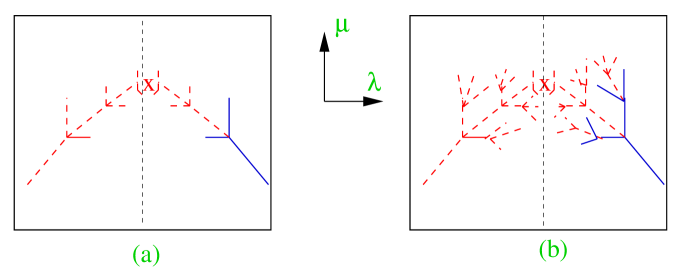
Figure 13: Possible behaviors around the merger point for $5\leq d<10$. (a) minimal change. (b) A fractal diagram. The thin dashed line separated the black hole phase on the right from the unstable string to the left. The number of negative modes for each phase is suppressed here.

The topology changing transition does not occur for $d<5$. Physically it is because that would require analyzing black holes in 3d and lower which do not have regular horizons but rather induce deficit angles, while mathematically it is because both sphere factors in ${\bf S}^{m}\times{\bf S}^{n}$ must have positive Einstein constant and so $m,\,n\geq 2$. For $5\leq d<10$ the picture stays similar to $d=5$.

However, for $d>10$ the previously tachyonic function stabilizes due to a competition in the action between the volume factor and a certain mass-like term. Closely related dependence on the dimension was observed in geometric studies of minimal cones [26]; in construction of cohomegeneity one Ricci flat metrics [27, 28]; in the stability of AdS compactifications over a product space [36] and [37] (this result could be related to this one by the cone-AdS relation [38], though here D brane probes do not exist as such); in [34] and in the stability of Schwarzschild black holes in a asymptotically conical background [35]. However, here they arise in a natural dynamical context for the first time. I can see no connection between the 10d criticality observed here and the critical dimension of superstring theory, and so if such a connection existed it would be very interesting.

A phenomenon that could remind one of the Gross-Witten transition as claimed in [3] was found, namely, that the free energy probably has a kink on the wall in configuration space where a topology change takes place (subsection 5.3). In 5d the jump is in the 3rd derivative (or higher), and in other dimensions it is at least $-2\,\mbox{Re}(s_{-})$ (figure 12). Moreover, a high order phase transition from black hole to non-uniform black string seems to occur at the merger point, but this is not a real phase transition, unless the emanating non-uniform black string is stable (which I do not expect). This issue should be revisited when the phase diagram in the vicinity of merger transition is better understood.

7.2 No Cusps

The cusps on the horizons which were discovered in numerical simulations of black hole collisions (see [7] and references therein) were not seen in the local model which has smooth minimal spheres. That seems to indicate that the cusps are velocity dependent, vanishing for a static configuration. It would be interesting to test this by measuring numerically the cusp for various relative velocities keeping equal separations. Another possibility is that the local model is not sensitive enough to detect the cusps.

7.3 Topology change

The term “topology change” in General Relativity is being used with several different meanings, for instance the topology of the whole space-time could change as a parameter is varied or the topology of a spatial slice could change as time progresses. The topology change here will be of the first kind, evolving with a parameter, just like the flop [40] and conifold [41] transitions for 6d Calabi-Yau surfaces. Expected implications for time evolution are briefly discussed below, and we should note that classical no-go theorems [45, 46] are not valid due to the presence of the singularity (somewhat in the flavor of the possible classical topology changes of [47]).

Let us compare the merger transition discussed here with the conifold transition [41] and the “$G_{2}$-conifold” [43, 44]. The merger transition is in $m+n+1$ dimensions and centers around the cone over ${\bf S}^{m}\times{\bf S}^{n}$ (minimum 5d) while the conifold ($G_{2}$-conifold) is in 6d (7d) involving the cone over ${\bf S}^{3}\times{\bf S}^{2}$ (${\bf S}^{3}\times{\bf S}^{3}$). Despite the similar topologies and Ricci flatness of the geometries they differ in supersymmetry and metric: whereas the previous topology changes had Killing spinors the merger cone does not, and indeed it is not even stable. Accordingly the metric on the spheres differs - the conifold ($G_{2}$-conifold) metric is given by the homogeneous space $T_{1,1}=(SU(2)\times SU(2))/U(1)$ ($SU(2)^{3}/SU(2)_{\mbox{diag}}$) whereas the merger cone involves the round spheres and in 6d can be written as $T_{1,0}=SU(2)/U(1)\times SU(2)$.

7.4 Future directions

I would like to point out the following topics for future work

• Phase diagram near the merger point.

• Lorentzian signature

• Explosive transition

• Uniqueness theorems (no hair)

• $\alpha^{\prime}$ corrections

• Merger and quantum gravity

which will be discussed below one by one.

The suggested phase diagram (figure 3) was found to require corrections near the merger point at least for $5\leq d<10$. Some possibilities were discussed above in subsection 7.1.

So far we worked only in the Euclidean signature, and it is an important question to understand the Lorentzian. The static solutions can be readily turned to static Lorentzian solutions outside the horizon, and one expects an extension into the inside of the horizon to exist. However, the singular cone solution at the merger transition will translate into a naked singularity on the horizon, at which point the structure of the light cone may be different and a problem with the extension of the solution could arise. Even more interesting is the time dependent behavior, when the tachyon decays. For instance, one could start with an unstable string $\mu<\mu_{GL}$ with initial conditions that as $t\to-\infty$, both the tachyon its time derivative approach zero $~{}T,\dot{T}\to 0$. Since the problem is time dependent the apparent horizon does not coincide anymore with the event horizon, and it would be interesting to understand the Penrose diagram.

The hysteresis curve contains two sections of tachyon decay, one starting after the Gregory-Laflamme point, and the other close to the merger transition. Since the energy emitted during these decays scales as the mass of the black object, it must equal a numerical constant times the mass (there are no dimensionless parameters at the transition points). Assuming large extra dimensions one finds large fusion/fission explosions [49].

The black hole uniqueness theorems (“no hair”), which characterizes a time-independent 4d black hole by its mass and angular momentum (and possibly gauge charges), does not hold as such for $d>4$. The 5d rotating black ring solution of [48] is a beautiful counter-example where for some values of the mass and angular momentum 3 solutions exist - 2 black rings and 1 black hole. The black-hole black-string transition provides another example for non-uniqueness above 5d, since at some values of $\mu$ there are at least 3 solutions - a (perturbatively) stable string, an unstable non-uniform string and the black hole. This example is static, but the asymptotic space-time is not Euclidean (though it is flat). It would be a shame to loose such a nice principle at higher dimension, and it would be better to try and “fix” it. Following this work a natural speculation arises - that the topology of the horizon must be specified, and that unstable solutions should not count [50].

It would be interesting to find string theoretic $\alpha^{\prime}$ corrections to the cone geometry. On the one hand large corrections could appear close to the tip where curvatures approach the string scale, but on the other hand the cone topology seems to be essential for the topology change, which may protect the cone. Perhaps non geometric modes become important like in the conifold transition [42].

Finally it is natural to wonder about the quantum gravity interpretation of a black hole merger, as mentioned in the introduction, and it is hoped that this work makes a step in that direction.

Acknowledgements

It is a pleasure to thank Lenny Susskind for introducing me to this problem some years ago; Gary Horowitz for rekindling my interest and for discussions; John Bahcall for encouragement; Tsvi Piran and Evgeny Sorkin for collaboration on a related project and comments on the paper; Sunny Itzhaki and Juan Maldacena for some enjoyable discussions; Steve Gubser, Igor Klebanov, Mukund Rangamani, Edward Witten for correspondence and important comments; David Berenstein, Sergey Cherkis, Eric Gimon and other members of the IAS group for discussions; and finally the University of California at Santa Barbara and Stanford university for hospitality while this work was in gestation.

The first version of this paper appeared while I was at the School of Natural Sciences, Institute for Advanced Study, Princeton and the work was supported by DOE under grant no. DE-FG02-90ER40542, and by a Raymond and Beverly Sackler Fellowship. Currently my work is supported in part by The Israel Science Foundation (grant no 228/02) and by the Binational Science Foundation BSF-2002160.

Appendix A Comments on a local analysis around the GL critical point

In this appendix I would like to describe an approach to the determination of the local properties of the system at the GL point which is somewhat different then the one used in [6] and is actually standard in the thermodynamics of phase transitions. It requires the computation of solutions up to the second order in perturbation rather than third, but the required hard computations were not pursued to the end.

Start by considering the action functional, namely working in the canonical ensemble. At the GL point the quadratic potential has one zero mode, and the objective is to go beyond the quadratic approximation, and determine whether this mode is negative or not, which are the only qualitative possibilities. This will determine the current goal, namely, whether the emerging phase is stable or not, and whether its $\mu$ starts climbing down or up.

The quadratic approximation to the action can be written as

$$-I_{2}[x,y_{i};{\hat{\mu}}]=k_{0}\,{\hat{\mu}}\,|x|^{2}+\sum_{i}m^{2}_{i}|y_{i}|^{~{}2}$$ (46)

where $x$ is the marginally stable mode, $y_{i}$ are all the other modes diagonalized such that their mass-squared are $m^{2}_{i}$, ${\hat{\mu}}=\mu-\mu_{GL}$ and $k_{0}$ is a positive constant. One would like to trace the emerging solutions $x,\,y_{i},\,{\hat{\mu}}$ as a function of a perturbation parameter $\epsilon$. Clearly at first order only $x$ can be turned on and the first task is to find it explicitly by solving the equations of motion for $I_{2}$.

Due to the $U(1)_{z}$ isometry of the uniform black-string all modes with $z$-dependence are complex with a specific charge $q_{i}$ such that under a rotation of the $z$ axis by an angle $\theta$ they transform by

$$y_{i}\to e^{q_{i}\,\theta}\,y_{i}$$ (47)

By the construction of $x$ we have $q_{x}=1$. Let us use the fact that the action is real and invariant under this action. The first consequence is that cubic terms involving only $x,\bar{x}$ (which would imply a first order transition) are forbidden. Therefore we must go to quartic order in $\epsilon$. For this we must expand the action to include

$$-I_{4}=\sum_{i}g_{i}\,y_{i}\,x^{2}+\mbox{c.c.}+\sum_{j}h_{j}\,y_{j}\,|x|^{2}+k\,|x|^{4}$$ (48)

where the sum is over modes of charge $\pm 2$ or 0 which couple to quadratics in $x,{\bar{x}}$ and $g_{i},\,h_{j}$ are the respective couplings.

One takes

$$x=x^{(1)}\,\epsilon+x^{(2)}\,\epsilon^{2}$$

$$y_{i}=y_{i}^{(2)}\,\epsilon^{2}$$ (49)

And finds that $-(I_{2}+I_{4})$ becomes a quadratic form in $\epsilon^{2}$, and its signature is determined by the sign of

$$k-\sum_{i}|g_{i}|^{2}/m^{2}_{i}-\sum_{j}h_{j}^{~{}2}/m^{2}_{j}$$ (50)

In practice it is more convenient to find the solution for $x,y_{i}$ up to second order in $\epsilon$ and check the sign of the resulting action $-(I_{2}+I_{4})$ - a positive mode means that it is a minimum and hence a second order phase transition will form, whereas a negative mode means that there is already another minimum lower than the present one, and so the system goes through a first order transition (see figure 8).

If one computes the constant $k_{0}$ in $I_{2}$ (46) one can solve for $\epsilon=\epsilon({\hat{\mu}})$ and extract quantitative information about the initial rates of change of $I,\,x,\,y_{i}$ along the new phase as a function of $\mu$.

References

- [1] R. Gregory and R. Laflamme, “Black Strings And P-Branes Are Unstable,” Phys. Rev. Lett. 70, 2837 (1993) [arXiv:hep-th/9301052].
- [2] R. Gregory and R. Laflamme, “The Instability of charged black strings and p-branes,” Nucl. Phys. B 428, 399 (1994) [arXiv:hep-th/9404071].
- [3] L. Susskind, “Matrix theory black holes and the Gross Witten transition,” [arXiv:hep-th/9805115].
- [4] D. J. Gross and E. Witten, “Possible Third Order Phase Transition In The Large N Lattice Gauge Theory,” Phys. Rev. D 21, 446 (1980).
- [5] G. T. Horowitz and K. Maeda, “Fate of the black string instability,” Phys. Rev. Lett. 87, 131301 (2001) [arXiv:hep-th/0105111].
- [6] S. S. Gubser, “On non-uniform black branes,” Class. Quant. Grav. 19, 4825 (2002) [arXiv:hep-th/0110193].
- [7] L. Lehner, “Numerical relativity: A review,” Class. Quant. Grav. 18, R25 (2001) [arXiv:gr-qc/0106072].
- [8] S. S. Gubser and I. Mitra, “The evolution of unstable black holes in anti-de Sitter space,” JHEP 0108, 018 (2001) [arXiv:hep-th/0011127].
- [9] H. S. Reall, “Classical and thermodynamic stability of black branes,” Phys. Rev. D 64, 044005 (2001) [arXiv:hep-th/0104071].
- [10] G. T. Horowitz and K. Maeda, “Inhomogeneous near-extremal black branes,” Phys. Rev. D 65, 104028 (2002) [arXiv:hep-th/0201241].
- [11] P. J. De Smet, “Black holes on cylinders are not algebraically special,” Class. Quant. Grav. 19, 4877 (2002) [arXiv:hep-th/0206106].
- [12] T. Wiseman, “Relativistic stars in Randall-Sundrum gravity,” Phys. Rev. D 65, 124007 (2002) [arXiv:hep-th/0111057].
- [13] G. T. Horowitz, “Playing with black strings,” arXiv:hep-th/0205069.
- [14] M. Choptuik, L. Lehner, I. Olabarrieta, R. Petryk, F. Pretorius, and H. Villegas, to appear.
- [15] T. Harmark and N. A. Obers, “Black holes on cylinders,” JHEP 0205, 032 (2002) [arXiv:hep-th/0204047].
- [16] V. E. Hubeny and M. Rangamani, “Unstable horizons,” JHEP 0205, 027 (2002) [arXiv:hep-th/0202189].
- [17] G. W. Kang, “On the stability of black strings / branes,” arXiv:hep-th/0202147.
- [18] D. Marolf and S. F. Ross, “Stringy negative-tension branes and the second law of thermodynamics,” JHEP 0204, 008 (2002) [arXiv:hep-th/0202091].
- [19] J. Geddes, “The collapse of large extra dimensions,” Phys. Rev. D 65, 104015 (2002) [arXiv:gr-qc/0112026].
- [20] R. Casadio and B. Harms, “Black hole evaporation and large extra dimensions,” Phys. Lett. B 487, 209 (2000) [arXiv:hep-th/0004004].
- [21] H. Weyl, “Zur Gravitationtheorie”, Annalen der Physik 54, 117-145 (1917).
- [22] D. J. Gross, M. J. Perry and L. G. Yafe, “Instability of at space at Finite temperature,” Phys. Rev. D 25, 330 (1982).
- [23] S. Wolfram, “Mathematica,” Wolfram Media and Cambridge University Press.
- [24] S. Hwang “A Rigidity Theorem for Ricci Flat Metrics,” Geometriae Dedicata 71, 5 (1998).
- [25] G. W. Gibbons, D. Ida and T. Shiromizu, “Uniqueness and non-uniqueness of static vacuum black holes in higher dimensions,” Prog. Theor. Phys. Suppl. 148, 284 (2003) [arXiv:gr-qc/0203004].
- [26] W. Y. Hsiang,“Minimal cones and the spherical Bernstein problem, II,” Invent. math. 74, 351-369 (1983).
- [27] C. Böhm, “Inhomogeneous Einstein metrics on low dimensional spheres and other low dimensional spaces,” Invent. math. 134, 145-176 (1998).
- [28] C. Böhm, “Non-compact cohomogeneity one Einstein manifolds,” Bull. Soc. math. France 127, 135-177 (1999).
- [29] J. -H. Eschenburg and M. Y. Wang, “The initial value problem for cohomogeneity one Einstein metrics,” J. Geom. Anal. 10, 109-137 (2000).
- [30] M. Rangamani and E. Witten, unpublished.
- [31] M. J. Duff, B. E. Nilsson and C. N. Pope, “The Criterion For Vacuum Stability In Kaluza-Klein Supergravity,” Phys. Lett. B 139, 154 (1984).
- [32] M. Berkooz and S. J. Rey, “Non-supersymmetric stable vacua of M-theory,” JHEP 9901, 014 (1999) [Phys. Lett. B 449, 68 (1999)] [arXiv:hep-th/9807200].
- [33] C. P. Herzog and I. R. Klebanov, “Gravity duals of fractional branes in various dimensions,” Phys. Rev. D 63, 126005 (2001) [arXiv:hep-th/0101020].
- [34] B. Kol, “Topology change in General Relativity, and the black-hole black-string transition”, circulated draft, June 21, 02.
- [35] G. Gibbons and S. A. Hartnoll, “A gravitational instability in higher dimensions,” Phys. Rev. D 66, 064024 (2002) [arXiv:hep-th/0206202].
- [36] O. DeWolfe, D. Z. Freedman, S. S. Gubser, G. T. Horowitz and I. Mitra, “Stability of AdS(p) x M(q) compactifications without supersymmetry,” Phys. Rev. D 65, 064033 (2002) [arXiv:hep-th/0105047].
- [37] T. Shiromizu, D. Ida, H. Ochiai and T. Torii, “Stability of AdS(p) x S(n) x S(q-n) compactifications,” Phys. Rev. D 64, 084025 (2001) [arXiv:hep-th/0106265].
- [38] I. R. Klebanov and E. Witten, “Superconformal field theory on threebranes at a Calabi-Yau singularity,” Nucl. Phys. B 536, 199 (1998) [arXiv:hep-th/9807080].
- [39] M. W. Choptuik, “Universality And Scaling In Gravitational Collapse Of A Massless Scalar Field,” Phys. Rev. Lett. 70, 9 (1993).
- [40] P. S. Aspinwall, B. R. Greene and D. R. Morrison, “Multiple mirror manifolds and topology change in string theory,” Phys. Lett. B 303, 249 (1993) [arXiv:hep-th/9301043]. P. S. Aspinwall, B. R. Greene and D. R. Morrison, “Calabi-Yau moduli space, mirror manifolds and spacetime topology change in string theory,” Nucl. Phys. B 416, 414 (1994) [arXiv:hep-th/9309097].
- [41] P. Candelas and X. C. de la Ossa, “Comments On Conifolds,” Nucl. Phys. B 342, 246 (1990).
- [42] A. Strominger, “Massless black holes and conifolds in string theory,” Nucl. Phys. B 451, 96 (1995) [arXiv:hep-th/9504090].
- [43] G. W. Gibbons, D. N. Page and C. N. Pope, “Einstein Metrics On S**3 R**3 And R**4 Bundles,” Commun. Math. Phys. 127, 529 (1990).
- [44] M. Atiyah and E. Witten, “M-theory dynamics on a manifold of G(2) holonomy,” Adv. Theor. Math. Phys. 6, 1 (2003) [arXiv:hep-th/0107177].
- [45] R. Geroch, “Topology in General Relativity,” J. Math. Phys. 8, 782 (1967).
- [46] F. Tipler, Ann. Phys. 108, 1 (1977).
- [47] G. T. Horowitz, “Topology Change In Classical And Quantum Gravity,” Class. Quant. Grav. 8, 587 (1991).
- [48] R. Emparan and H. S. Reall, “A rotating black ring in five dimensions,” Phys. Rev. Lett. 88, 101101 (2002) [arXiv:hep-th/0110260].
- [49] B. Kol, “Explosive black hole fission and fusion in large extra dimensions,” arXiv:hep-ph/0207037.
- [50] B. Kol, “Speculative generalization of black hole uniqueness to higher dimensions,” arXiv:hep-th/0208056.
- [51] B. Kol, “Topology change in general relativity and the black-hole black-string transition,” arXiv:hep-th/0206220.
- [52] B. Kol, “The phase transition between caged black holes and black strings: A review,” arXiv:hep-th/0411240.