LBNL-50597

UCB-PTH-02/25

UFIFT-HEP-02-20

hep-th/0206205

A Mean Field Approximation to the
Worldsheet Model of Planar $\phi^{3}$ Field Theory
Korkut Bardakci
Department of Physics, University of California at Berkeley
and
Theoretical Physics Group, Lawrence Berkeley National Laboratory
University of California, Berkeley CA 94720
and
Charles B. Thorn
School of Natural Sciences, Institute for Advanced Study, Princeton NJ 08540
and
Institute for Fundamental Theory
Department of Physics, University of Florida, Gainesville FL 32611

We develop an approximation scheme for our worldsheet model of the sum of planar diagrams based on mean field theory. At finite coupling the mean field equations show a weak coupling solution that resembles the perturbative diagrams and a strong coupling solution that seems to represent a tensionless soup of field quanta. With a certain amount of fine-tuning, we find a solution of the mean field equations that seems to support string formation.

1 Introduction

Last year we initiated a program [1], for summing the planar graphs of large $N_{c}$ matrix field theories, based on a description of each planar diagram as a light-cone worldsheet path integral. Once this worldsheet representation was obtained, we could then realize the sum over planar graphs by coupling the worldsheet matter and ghost fields to a two dimensional Ising spin system. Summing over all spin configurations accomplishes the sum over all planar diagrams. One can regard the resulting two dimensional system as a noninteracting string moving in a background described by the Ising spin system. In this way our proposal arrives at a result suggested by the Maldacena conjecture [2], namely the association of a free string theory in a non-trivial background with the sum of planar diagrams. But instead of relying on open-string/closed-string duality to provide equations for the background, we are able to “read off” the background directly from the planar diagrams being summed. Thus we hope our approach represents an attack on the problem of large $N_{c}$ QCD complementary to the well studied AdS/CFT duality.

The worldsheet construction of [1] was restricted to $\phi^{3}$ scalar field theory, but the methods were soon extended to the important case of pure Yang-Mills field theory in [3]. The extension to supersymmetric field theories remains to be done. But here we return to the simple $\phi^{3}$ theory as a useful arena for developing methods for extracting the physical properties of the worldsheet system, and hence those of the large $N_{c}$ limit. In particular we wish to apply the mean field approximation to the Ising spin system in order to get a qualitative understanding of the basic physics described by the sum of planar graphs. Such an approach has previously been applied in an attempt to extract nonperturbative information from lattice string theory [4] in Ref. [5].

At the outset we should take note of the fundamental instability of $\phi^{3}$ theory following from the unboundedness of the cubic potential. As long as the free fields we perturb around are not tachyonic, this instability does not obstruct the evaluation of any Feynman graph, nor does it prevent one from contemplating graph summation [6]. Although our real interest is summing the planar diagrams of a stable non-abelian gauge theory, we find the simplicity of $\phi^{3}$ diagrams particularly valuable as a toy system for developing and testing our methodology. In particular, we can ask whether our methods are at all sensitive to the instabilities we know are there. There is even the possibility that a metastable vacuum in the finite $N_{c}$ case becomes stable in the $N_{c}\rightarrow\infty$ limit [7]. If so, the planar sum might give a physically meaningful answer, and show instability only at higher order in the $1/N_{c}$ expansion.

We develop the mean field method in stages. After a brief review of the worldsheet formalism in Section 2, we begin in Section 3 with a treatment motivated by the formal continuum limit of the worldsheet model. The qualitative continuum physics is reviewed and the mean field is introduced. The basic idea is that the three worldsheet systems in the construction, namely the target space variables ${\bf q}$ the ghosts $b,c$ and the Ising spins $s$, are first exactly solved in the presence of a homogeneous mean field. Then the value of the mean field is determined by minimizing the sums of the energies of the three systems. Because the mean field $\phi$ is supposed to represent a fundamental variable that only takes on the values $0$ or $1$, there is some freedom in the way it can enter the dynamics, when $0<\phi<1$, in the first approximation to the actions that describe the target space and ghost systems. Postponing this issue to Section 4, we instead use simple scaling arguments to fix a reasonable interpolation for the mean ghost$+$matter energy between its values for $\phi=0$ and $\phi=1$. The resulting mean field equation has a solution that supports string formation for a certain choice of parameters. For this choice there is a minimum of the energy that is associated with a finite non-zero string tension.

In Section 4, we develop the mean field approach directly from the lattice system that was the foundation of our mapping of planar diagrams to worldsheets. This treatment is thus more transparently related to the original field theoretic perturbation theory. Here we identify the mean field approximation as a certain saddle-point evaluation of the path integral. In this context, the ambiguities mentioned in the previous paragraphs are simply rearrangements of the path integration that are valid in the exact integral but lead to differences in the saddle-point approximation. Since the saddle-point approximation can be systematically corrected, there is an objective criterion for choosing the zeroth order action, namely the one for which the corrections are as small as possible. We base our choice in this section on how well it works at zero coupling, where exact calculations can be made. It turns out that the consequences of this choice are qualitatively very similar to the results of Section 3. The main difference can be traced to the $\phi^{3/2}$ dependence of the energy in (51), as opposed to the linear dependence on $\phi$ in (28). This is due to the ambiguities in the application of the saddle point method mentioned above, and it does not lead to any qualitative change in the final results. Again there is a range of parameters, where the coupling ${\hat{g}}=O(\epsilon)$ where the effective string tension is finite and non-zero. Here $\epsilon$ is a temporary infrared cutoff that must be sent to $0$. Although the coupling is tending to $0$, this is not the perturbative regime, which is obtained by expanding about $g=0$ at fixed $\epsilon$ and lattice cutoffs, and only removing the cutoffs order by order at the end of the calculation. For $g/\epsilon\rightarrow 0$ the effective string tension becomes infinite, signaling the return to the perturbative region of weakly coupled field quanta.

For $g=O(1)$ as $\epsilon\rightarrow 0$, the effective tension in our approximation is $0$: the system is some kind of tensionless soup. We believe that the unphysical nature of this regime is a reflection of the inherent instability of the initial $\phi^{3}$ theory. We find the existence of a regime with string formation interesting, even though it seems to require a certain amount of fine-tuning.

Concluding remarks are given in Section 5. We also include two appendices. In the first we explain the tools for evaluating the Gaussian path integrals encountered throughout the article. In the second, we discuss a simple extension of the mean field description to slowly varying fields.

2 Review of the Worldsheet Formalism for Field Theory

The light-front components of any Minkowski vector $v^{\mu}$ will be written $(v^{+},v^{-},{\bf v})$ or $(v^{+},v^{-},v^{k})$. Here $v^{\pm}=(v^{0}\pm v^{3})/\sqrt{2}$, and the remaining components label the transverse directions. The Lorentz invariant scalar product of two four vectors $v,w$ is written $v\cdot w={\bf v}\cdot{\bf w}-v^{+}w^{-}-v^{-}w^{+}$. We shall select $x^{+}$ to be our quantum evolution parameter, and we recall that the Hamiltonian conjugate to this time is $p^{-}$. A massless on-shell particle thus has the “energy” $p^{-}={\bf p}^{2}/2p^{+}$.

The starting point for the worldsheet construction [1] is the path integral representation of the (imaginary time) light-cone evolution operator for a free particle or field quantum

$$\exp\left\{-{\tau\over 2p^{+}}{({\bf q}_{M}-{\bf q}_{0})^{2}}\right\} = \int DcDbD{\bf q}\ e^{-S_{0}}$$ (1)

$$S_{0} = \int_{0}^{\tau}d\tau\int_{0}^{p^{+}}d\sigma\left(b^{\prime}c^{\prime}-{1\over 2}{\bf q}^{\prime 2}\right),$$ (2)

where the prime denotes $\partial/\partial\sigma$, and where Dirichlet boundary conditions ${\bf q}(0,\tau)={\bf q}_{0}$, ${\bf q}(p^{+},\tau)={\bf q}_{M}$, $b=c=0$ are imposed on the world sheet fields. The target space coordinates ${\bf q}(\sigma,\tau)$ are related to the transverse momentum carried by the system by ${\bf p}=\int_{0}^{p^{+}}d\sigma{\bf q}^{\prime}={\bf q}_{M}-{\bf q_{0}}$, and the Dirichlet boundary conditions on ${\bf q}$ ensure the conservation of total momentum. The ghosts $b,c$, which are Grassmann variables, are necessary to ensure the correct measure factors. We shall always understand path integrals to be the continuum limit of ordinary integrals over variables defined on a lattice [4]. We specify the lattice spacing in $\tau$ to be $a$ and that in $\sigma$ to be $m$. The continuum limit will be $a,m\rightarrow 0$ with $m/a$ fixed. Then the measure of the path integral is given by

$$DcDbD{\bf q}\equiv\prod_{j=1}^{N}\prod_{i=1}^{M-1}{dc_{i}^{j}db_{i}^{j}\over 2\pi}{d{\bf q}_{i}^{j}},$$ (3)

where $\tau=Na$ and $p^{+}=Mm$, with $M,N$ large positive integers. Note that since $\sigma$ has dimensions of momentum and $\tau$ has dimensions of time, $m/a$ has the dimensions of force.

As discussed in [1], a general planar diagram in quantum field theory can be represented as a path integral similar to (2) but with any number of internal Dirichlet boundaries given by any number of parallel line segments at fixed $\sigma$, summed over varying location and length. Cubic vertices are simply represented by the appearance or disappearance of a Dirichlet boundary, and so are characterized locally on the world sheet. Vertices of higher order are represented by the simultaneous appearance and disappearance of more than one Dirichlet boundary, and hence involve nonlocal constraints on the geometry of the world sheet.

If we follow a line at fixed $\sigma$ in a general planar diagram, we find a sequence of appearances and disappearances of Dirichlet boundaries. Thus each such line is associated with a two state system: the Dirichlet boundary is either “on” (solid line) or “off” (dotted line). Thus, in addition to the target space and ghost worldsheet fields, we also introduce an Ising spin variable $s_{i}^{j}=\pm 1$ at each site of the worldsheet lattice. A time link joining two $+$ spins is a bit of Dirichlet boundary, and one joining two $-$ spins is a bit of bulk. A time link joining opposite sign spins is a spin flip that turns a bit of Dirichlet boundary on or off. The sum over all spin configurations then accomplishes the sum over all planar diagrams.

In practice, the specification of the interacting Ising/target space system involves case by case technical details, given for $\phi^{3}$ theory in [1] and for Yang-Mills in [3]. Here we only quote the final proposal for the $\phi^{3}$ theory which is the focus of the rest of this article. The amplitude for the sum of all planar diagrams evolving an initial state $i$ to a final state $f$ is given by

$$T_{fi} = \lim_{\epsilon\rightarrow 0}\sum_{s_{i}^{j}=\pm 1}\int DcDbD{\bf q}\exp\left\{{{a\over 2m\epsilon}\sum_{i,j}b_{i}^{j}c_{i}^{j}\sqrt{2m\epsilon\over a\pi}\left[{\cal V}_{0i}^{j}{\cal P}_{i}^{j}+{\bar{\cal V}}_{0i}^{j}{\bar{\cal P}}_{i}^{j}\phantom{\sum}\hskip-14.22636pt\right]}\right\}$$

$$\exp\left\{-{a\over 2m}\sum_{i,j}\left[({\bf q}_{i+1}^{j}-{\bf q}_{i}^{j})^{2}+{({\bf q}_{i}^{j}-{\bf q}_{i}^{j-1})^{2}}{P_{i}^{j}P_{i}^{j-1}\over\epsilon}\right]+\sum_{i,j}{a\over m\epsilon}P_{i}^{j-1}P_{i}^{j}P_{i}^{j+1}b^{j}_{i}c^{j}_{i}\right\}$$

$$\exp\left\{{a\over m}\sum_{i,j}\left[(b_{i+1}^{j}-b_{i}^{j})(c_{i+1}^{j}-c_{i}^{j})(1-P_{i}^{j})(1-P_{i+1}^{j})+(1-P_{i}^{j})(P_{i+1}^{j}+P_{i-1}^{j})b_{i}^{j}c_{i}^{j}\right]\right\},$$

where $P_{i}^{j}=(1+s_{i}^{j})/2$ and we have put $\epsilon=m\epsilon/a$. The states $|i\rangle,|f\rangle$ are specified by the number and position of Dirichlet boundaries that extend to $\tau=-\infty,+\infty$ respectively. Here the vertex functions are given by

$${\cal V}_{0i}^{j} \equiv {ga\over 4m\sqrt{\pi}}\exp\left\{-{a\over m}(b_{i-1}^{j}c_{i-1}^{j}+b_{i+1}^{j}c_{i+1}^{j})\right\}$$

$${\bar{\cal V}}_{0i}^{j} \equiv {ga\over 4m\sqrt{\pi}}\exp\left\{-{a\over m}(b_{i+1}^{j+1}-b_{i}^{j+1})(c_{i+1}^{j+1}-c_{i}^{j+1})\right\}.$$ (5)

Also the projectors multiplying the vertex functions are

$${\cal P}_{i}^{j}\equiv P_{i}^{j}P_{i}^{j+1}(1-P_{i}^{j-1})\Pi_{i-1}^{j-1}\Pi_{i+1}^{j-1},\qquad{\bar{\cal P}}_{i}^{j}\equiv P_{i}^{j}P_{i}^{j-1}(1-P_{i}^{j+1})\Pi_{i-1}^{j}\Pi_{i+1}^{j},$$ (6)

where $\Pi_{i}^{j}\equiv(1+s_{i}^{j}s_{i}^{j+1})/2$.

Without going into great detail we make a few explanatory comments about this formula. First, notice that the spin projectors $P_{i}^{j}$ keep track of the distinction between solid ($P=1$) and dotted ($P=0$) lines. A bit of Dirichlet boundary is represented by a delta function, identifying the ${\bf q}$’s at successive sites, defined through the limit

$$\delta(\Delta{\bf q})=\lim_{\epsilon\rightarrow 0}\left({a\over 2\pi m\epsilon}\right)^{D/2}e^{-a\Delta{\bf q}^{2}/2m\epsilon}.$$ (7)

The prefactors in this formula are taken care of by the ghost integration. Since formally $\delta({\bf 0})=V_{\perp}/(2\pi)^{D}$, the volume of transverse space, we should regard $\epsilon$ as a temporary infrared cutoff on the transverse coordinates, related to the size of the space $L=V^{1/D}$ by $\epsilon=2\pi a/mL^{2}$. The different arrangement of projectors for ghosts compared to those for ${\bf q}$ is due to the fact that $b=c=0$ on solid lines, whereas the ${\bf q}$’s are only required to be equal on solid lines. The apparently elaborate ghost dependence of the vertex functions in (5) provides necessary factors of $1/p^{+}$ that are dictated by the field theoretic Feynman rules. The noteworthy feature is that in spite of their complexity, they are described locally on the world sheet. The rather complicated combination of projectors multiplying these vertex functions limits their occurrence to the appearance or disappearance of Dirichlet boundaries. The extra $\Pi$ projectors remove difficulties, due to the ghost insertions in (5), that occur when two or more vertices are within one or two lattice sites of each other.

Finally we comment on the limits involved in recovering standard field theoretic perturbation theory from Eq. 2. One first expands the formula in a power series in $g$, $T=\sum_{n}g^{n}T_{n}(\epsilon,a,m)$. Then the limit $\epsilon\rightarrow 0$ on each $T_{n}$ converts it to a standard Feynman integral, with uv cutoff $a$ and $p^{+}$ cutoff $m$. The dependence on these cutoffs then just parameterizes the standard field theoretic divergences. In this article we are attempting to learn about physics at finite coupling by studying (2) in the presence of all these cutoffs. But to compare our results to perturbation theory we must keep in mind that the perturbation expansion is carried out before sending $\epsilon\rightarrow 0$, implying the parametric regime $g\ll\epsilon$.

3 The Mean Field Approximation on a Continuous Worldsheet with Simple Cutoff

In this section, we will develop a somewhat crude, but qualitatively transparent, version of the mean field method on the world sheet. A more precise and detailed version of the same method, based on the worldsheet lattice, will be presented in the next section. Here we will adopt the continuum version of the world sheet, and we will use the notation and conventions of the previous section, except that we use the Minkowski metric in both target space (so the factor at each vertex is $ig$, $g=$coupling const.) and on the world sheet. The worldsheet coordinate $\sigma$ is compactified in the interval 0 to $p^{+}$, and $\tau$ runs over the interval $\tau_{i}$ to $\tau_{f}$, which will eventually go to infinity. The target space fields ${\bf q}(\sigma,\tau)$, which will be designated as matter fields, live in $D$ dimensions. For simplicity, we take the total transverse momentum flowing through the worldsheet to be zero:

$$\int^{p^{+}}_{0}d\sigma{\bf q^{\prime}(\sigma,\tau)}={\bf q}(p^{+},\tau)-{\bf q}(0,\tau)=0.$$

To keep track of the two types of lines, it is convenient to define a scalar field $\phi$ on the worldsheet which is 1 on solid lines and 0 on dotted lines. Now consider the expression

$$\left(i\beta\phi\over\pi\right)^{D/2}\,\exp\left(-i\beta\phi({\bf V})^{2}\right)$$ (8)

As $\beta$ tends to $\infty$, this expression tends to a delta function, $\delta({\bf V})$, for all $\phi\neq 0$. Here, we assume a Euclidean continuation to have a well defined Gaussian. We will use this to impose the condition

$$\dot{{\bf q}}=0$$

on solid lines, where $\phi=1$. On dotted lines, where $\phi=0$, there is no constraint. The matter part of the action, with the above constraint, takes the form

$$S_{q} = \int_{0}^{p^{+}}d\sigma\int_{\tau_{i}}^{\tau_{f}}d\tau\,\mathcal{L}_{q},$$

$$\mathcal{L}_{q} = \frac{1}{2}\beta\phi(\dot{{\bf q}})^{2}-\frac{1}{2}({\bf q}^{\prime})^{2}.$$ (9)

For the time being, we will keep the parameter $\beta$ finite, though eventually we will let $\beta\rightarrow\infty$. Comparing to the lattice expression (2), we see that $\phi$ here is playing the role of the projectors $P_{i}^{j}P_{i}^{j-1}$, and $\beta=a^{2}/m^{2}\epsilon$. Also, we have dropped the prefactors in front of the exponential in (8); these give rise to quantum effects which will not play a role in the approximate treatment of this section. However, their effect will be included in the lattice calculations of Sec. 4, where we shall see that they are mostly canceled by corresponding factors in the ghost sector.

In addition to the matter part of the action, there is the ghost action. The function of ghosts is to cancel the contribution of the matter fields on the dotted lines, and leave it untouched on solid lines. The ghost action is somewhat complicated, and its lattice version will be given in the next section. For our purposes, we will not need the explicit form of the ghost action. In fact, we find it easier to compute directly the effective actions $W_{q,g}(\phi)$ for matter and ghost sectors as a function of $\phi$. The calculation proceeds as follows: The world sheet can be thought of as a union of black regions, composed of only the solid lines, and the white regions, composed of only the dotted lines (See Fig.1).

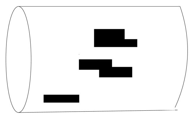
Figure 1: Regions of Worldsheet

In the white regions, where $\phi=0$, the situation is very simple: The matter and the ghost contributions cancel, and the total effective action is zero:

$$W_{q}(\phi=0)+W_{g}(\phi=0)=0.$$ (10)

On the other hand, in the black regions, where $\phi=1$, the ghosts do not contribute:

$$W_{g}(\phi=1)=0.$$ (11)

Therefore, we need only compute $W_{q}(\phi=1)$ for an arbitrarily shaped black region. This is a standard Casimir type calculation. Since the answer is divergent, a suitable cutoff has to be introduced, and for the Casimir effect, one has to calculate the cutoff independent finite part. Here, we have a much simpler problem: We are interested in the dominant bulk contribution to the action, which is going to be the leading cutoff dependent term. It is also going to be proportional to the area of the black region and independent of its shape. We will compute this term for a rectangular black region of width $L$ in the $\sigma$ direction and length $T$ in the $\tau$ direction, taking $\phi$ to be a constant ($\sigma$ and $\tau$ independent) in Eq.(9). We will also impose periodic boundary conditions in both directions and use a cutoff in the mode number. Defining the operator $K$ by

$$K=\beta\phi\partial_{\tau}^{2}-\partial_{\sigma}^{2},$$

we have

$$W_{q}=-\frac{D}{2}{\rm Tr}\log(K).$$ (12)

The cutoff dependent part of the action is easily calculated:

$$W_{q}\cong-\frac{D\,LT}{4\pi(\beta\phi)^{1/2}\delta}.$$ (13)

Here $\delta$, which has the dimensions of $\sigma^{2}$, is the cutoff parameter. It is proportional to $m^{2}$, where $m$ is the discrete unit of $\sigma$ on the world sheet lattice.

We note that the answer depends only on the area $LT$ of the region. Although the calculation was done for a rectangular region, it is clear that the leading cutoff dependent term is proportional to the area even for a region of an arbitrary shape, and independent of the boundary conditions imposed. This dependence on the area, and also the dependence on the combination $\beta\phi$, can be established essentially by dimensional and scaling arguments, independent of any detailed calculation. The numerical factor $4\pi$ is unimportant and it could be absorbed into the definition of the cutoff. For small sized regions perimeter and shape dependent contributions may also become important. However, in this section, we will focus on the bulk contribution only, and we will neglect corrections of this type. The cutoff $\delta$ hides our ignorance of the texture of the world sheet when the continuum limit is taken; it will eventually be absorbed into the definition of the coupling constant. Finally, the matter contribution to the action in the black region is obtained by setting $\phi=1$ in Eq.(13):

$$W_{q}(\phi=1)=-\frac{D\,A}{4\pi(\beta)^{1/2}\delta},$$ (14)

where $A$ is the area of the region. Eqs.(10),(11) and (14) provide us with complete information about the contributions of the matter and ghost actions in the two types of regions.

Next, we have to tackle the functional integration over $\phi$. We impose the constraint that $\phi=0,1$ by means of a Lagrange multiplier $\pi(\sigma,\tau)$:

$$\Delta S_{n} = \int_{0}^{p^{+}}d\sigma\int_{\tau_{i}}^{\tau_{f}}d\tau\,\Delta\mathcal{L}_{n},$$

$$\Delta\mathcal{L}_{n} = \pi\left(\dot{\phi}-\sum_{1}^{n}(-1)^{m}\delta(\tau-\tau_{m}(\sigma_{0}))\right).$$ (15)

The functional integration over $\phi$ consists of integration over $\tau_{m}(\sigma_{0})$ and summation over n. These summations and integrations cannot be carried out in closed form; however, the problem can be reduced to the solution of a differential equation. Let us set

$$\exp\left(\Delta S^{i,j}\right)=F^{i,j}(\tau_{i},\tau_{f}),$$

where $\Delta S^{i,j}$ is the resulting action after the sums and integrals are carried out. The outcome is one of the four possible functions on the right hand side, depending on the boundary conditions on $\phi$ at $\tau_{i}$ and $\tau_{f}$. The indices $i$ and $j$ can take on the values ($+$) or ($-$), corresponding to $\phi=1,0$ at $\tau=\tau_{i,f}$. These functions are defined through the differential equations

$$\partial_{\tau}F^{+,+}(\tau_{i},\tau) = ig\>\exp\left(i\pi(\tau)\right)\,F^{+,-}(\tau_{i},\tau),$$

$$\partial_{\tau}F^{+,-}(\tau_{i},\tau) = ig\>\exp\left(-i\pi(\tau)\right)\,F^{+,+}(\tau_{i},\tau),$$

$$\partial_{\tau}F^{-,+}(\tau_{i},\tau) = ig\>\exp\left(i\pi(\tau)\right)\,F^{-,-}(\tau_{i},\tau),$$

$$\partial_{\tau}F^{-,-}(\tau_{i},\tau) = ig\>\exp\left(-i\pi(\tau)\right)\,F^{-,+}(\tau_{i},\tau),$$ (16)

plus the initial conditions

$$F^{+,+}(\tau_{i}=\tau_{f}) = F^{-,-}(\tau_{i}=\tau_{f})=0,$$

$$F^{+,-}(\tau_{i}=\tau_{f}) = F^{-,+}(\tau_{i}=\tau_{f})=1.$$ (17)

In writing these equations, we have assumed that the vertex that converts a dotted line into a solid line or vice versa is simply given by the coupling constant $g$. It was shown in [1] that there are additional contributions to the vertex involving the ghosts $b$ and $c$; however, in the leading large $D$ limit, which will be the approximation scheme adopted in this article, they do not contribute. This is because the function of these vertex ghost insertions is to produce the factor of $1/p^{+}$, which is part of the propagator, and it does this by deleting a pair of ghost fields $b$ and $c$, as explained in [1]. The crucial point is that it is always a pair of fields irrespective of the transverse dimension $D$, since $p^{+}$ always appears to the first power and not to the power $D$. Therefore, this contribution goes like 1 and not $D$, and it is negligible in the large $D$ limit. We will have more to say about the large $D$ limit later.

It turns out to be convenient, although not essential, to keep track of the $(+)$ and ($-$) indices by means of two fermionic (anticommuting) variables $e_{1,2}(\tau,\sigma)$. These fermions, already introduced in [1], give the continuum formulation of the Ising system of the next section. $e_{1}$ is associated with the $(+)$ index, or the solid lines, and $e_{2}$ with the ($-$) index, or the dotted lines. Their $\tau$ dependence is given by

$$e_{1}(\tau,\sigma) = F^{+,+}(\tau_{i},\tau)e_{2}(\tau_{i},\sigma)+F^{-,+}(\tau_{i},\tau)e_{1}(\tau_{i},\sigma),$$

$$e_{2}(\tau,\sigma) = F^{+,-}(\tau_{i},\tau)e_{2}(\tau_{i},\sigma)+F^{-,-}(\tau_{i},\tau)e_{1}(\tau_{i},\sigma).$$ (18)

As a result, the $e$’s satisfy the differential equations

$$i\dot{e}_{1}+g\;\exp(i\pi(\tau))e_{2} = 0,$$

$$i\dot{e}_{2}+g\;\exp(-i\pi(\tau))e_{1} = 0,$$ (19)

leading to the action

$$S_{f}=\int_{0}^{p^{+}}d\sigma\int_{\tau_{i}}^{\tau_{f}}d\tau\left(i\bar{e}_{1}\dot{e}_{1}+i\bar{e}_{2}\dot{e}_{2}+g\;\exp(i\pi)\bar{e}_{1}e_{2}+g\;\exp(-i\pi)\bar{e}_{2}e_{1}\right).$$ (20)

For later application, it is convenient to make the change of variables,

$$e_{1} = \exp\left(\frac{i}{2}\pi\right)\psi_{1},\;\bar{e}_{1}=\exp\left(-\frac{i}{2}\pi\right)\bar{\psi}_{1},$$

$$e_{2} = \exp\left(-\frac{i}{2}\pi\right)\psi_{2},\;\bar{e}_{2}=\exp\left(\frac{i}{2}\pi\right)\bar{\psi}_{2},$$ (21)

with the corresponding action

$$S_{f}=\int_{0}^{p^{+}}d\sigma\int_{\tau_{i}}^{\tau_{f}}d\tau\left(i\bar{\psi}_{1}\dot{\psi}_{1}+i\bar{\psi}_{2}\dot{\psi}_{2}-\frac{1}{2}\dot{\pi}\,\bar{\psi}_{1}\psi_{1}+\frac{1}{2}\dot{\pi}\,\bar{\psi}_{2}\psi_{2}+g\,\bar{\psi}_{1}\psi_{2}+g\,\bar{\psi}_{2}\psi_{1}\right).$$ (22)

Adding all the contributions, the full expression for

$$T_{fi}=\langle{\bf p}_{f}|e^{-\tau p^{-}}|{\bf p_{i}}\rangle$$

is

$$T_{fi} = \int D{\bf q}\,D\lambda\,D\phi\,Db\,Dc$$ (23)

$$\times\exp\left(i\int_{0}^{p^{+}}d\sigma\int_{\tau_{i}}^{\tau_{f}}d\tau(\mathcal{L}_{q}+\mathcal{L}_{g}+\mathcal{L}_{f}-\dot{\pi}\phi)\right),$$

where $\mathcal{L}_{q}$ and $\mathcal{L}_{f}$ are given by Eqs.(9) and (22).

We are interested in the ground state of the system described by the action given above. We will compute the ground state of the combined matter, ghost and the fermionic systems in the presence of constant fixed background fields $\phi$ and $\pi$, and then minimize the total energy with respect to these background fields by solving the classical equations of motion. This is in essence the mean field method. A systematic way to do this is to consider the large $D$ limit, where $D$ is the number of transverse dimensions. In practice, this number is not particularly large, so the method could at best be expected to give qualitative results. However, it is a convenient way of organizing a systematic expansion scheme in inverse powers of $D$. We note that the contributions of the matter and ghost fields to the ground state energy are proportional to $D$, so it is convenient to scale the field $\pi$ and the coupling constant $g$ by

$$\pi\rightarrow D\pi,\;g\rightarrow Dg,$$ (24)

in order to have an effective action proportional to $D$. In what follows, we will simplify things by considering only the leading contribution in $D$. This does not mean that the non-leading contributions are unimportant; for example, it is clear that Lorentz invariance can only be understood by taking into account the non-leading terms. Also, there is the question of the meaning of the coupling constant $g$. From Eq.(16), one sees that this constant always has the dimensions of mass (or energy). The dimension of the constant $g$ that appears in the $g\,\phi^{3}$ interaction in field theory is ${\rm mass}^{(4-D)/2}$, depending on the dimensionality of space-time; only for $D=2$ (4 dimensional space-time), does it have the dimensions of mass. As a result, we cannot identify the constant $g$ that we are using with the field theory coupling constant, except perhaps in four dimensional space-time. In other dimensions, we have to treat it as an effective parameter, and to establish its connection with the parameters in field theory would again require a knowledge of higher order terms in the $1/D$ expansion On the light-cone worldsheet $\sigma$ has dimensions of momentum and $\tau$ the dimensions of time. On our worldsheet lattice, the lattice constants in the two directions therefore have a dimensionful ratio $m/a$, with dimensions of force. Since this ratio may be kept fixed in the limit of a continuous world sheet, the formalism provides a scale which can be used to define a dimensionless coupling constant. ${\hat{g}}\equiv g\sqrt{1/32\pi^{2}}(a/m)^{(4-D)/4}$. The coupling constant used in (16) can therefore be identified with ${\hat{g}}(m/a)^{(4-D)/4}$ up to dimensionless factors.

Another important simplification follows from the nature of the ground state. Since the problem is translationally invariant in both the compactified $\sigma$ and the $\tau$ direction, at least in the limit $\tau_{f}-\tau_{i}\rightarrow\infty$, we expect the ground state to share these symmetries; therefore, we take $\phi_{0}$, the expectation value of $\phi$, to be independent of $\sigma$ and $\tau$. We note that the value of the product $\beta\phi_{0}$ is especially significant: From Eq.(9), it follows that a finite non-zero value of this product leads to the standard string action with a finite slope parameter. The key idea behind our computation is self consistency. Starting with a finite $\beta\phi_{0}$, we compute the zero point energy of the resulting string, and add this to the energy of the fermions to get the total energy. Minimizing this energy, we arrive at a finite value of $\beta\phi_{0}$, completing the cycle of self consistency.

In trying to compute the energy of the combined matter and ghost system for a background value $\phi_{0}$ of $\phi$, we encounter a problem. We know the effective action for this system, from which the ground state energy is easily deduced, only for $\phi=0$ and $\phi=1$ (Eqs.(10),(11), and (14)). On the other hand, $\phi_{0}$ can take on any value between 0 and 1, so we have to extend the definition of the action to an arbitrary $\phi_{0}$ between these limits. This can be done as follows: $\phi_{0}$ is the classical expectation value, or the average value of $\phi$. Consider a specific partitioning of the world sheet between the white and black regions, such as represented by figure 1. If we denote the total area of the black regions by $A_{b}$ and the total area of the world sheet by $A_{w}$, and remembering that $\phi=0$ on the white regions and $\phi=1$ on the dark regions, the average value of $\phi$, $\phi_{0}$, for this partitioning is given by

$$\phi_{0}=\frac{A_{b}}{A_{w}}.$$ (25)

On the other hand, from Eqs.(10),(11) and (14), the contribution of this partitioning to the combined matter and ghost action is

$$W_{q}+W_{g}=-\frac{D\,A_{b}}{4\pi(\beta)^{1/2}\delta}.$$ (26)

From these equations, it follows that

$$W_{q}+W_{g}=-\frac{DA_{w}\,\phi_{0}}{4\pi(\beta)^{1/2}\delta},$$ (27)

which is the equation that expresses the combined action in terms of $\phi_{0}$. It is now easy to convert this into an equation for the corresponding ground state energies, which we label as $E_{q}^{(0)}$ and $E_{g}^{(0)}$ respectively. Remembering that the area of the world sheet is given by

$$A_{w}=p^{+}(\tau_{f}-\tau_{i}),$$

we have,

$$E_{q}^{(0)}+E_{g}^{(0)}=\frac{D\,p^{+}\phi_{0}}{4\pi(\beta)^{1/2}\delta}.$$ (28)

The combined matter and ghost energy therefore has a simple linear dependence on $\phi_{0}$. This is a direct consequence of the area law for the matter action (see Eq.(14)). Since this simple dependence on area is bound to get corrections for small regions, we expect to have some deviation from the linear dependence of the energy on $\phi_{0}$. In fact, a calculation based on the worldsheet lattice, presented in the next section, results in a more complicated dependence, but the linear dependence can be regarded as a reasonable approximation.

Next, we have to introduce some background for the field $\pi$. At first, one might think that, by translation invariance, this should again be a constant. However, it turns out that a constant background is trivial; it is clear from Eq.(22) that only the derivative of $\pi$ with respect to $\tau$ has dynamical significance. So we ansatz

$$\langle\pi\rangle\cong\pi^{(0)}(\tau)=\pi_{0}\tau+\pi_{1},$$ (29)

where $\pi_{0,1}$ are constants. Again, we see from Eq.(22) that this background, which at first looks time dependent, is in fact static, and the system has a well defined energy. To compute this energy, it is convenient to quantize the fermion action of Eq.(22), in the background given by Eq.(29), and construct the Hamiltonian. The result is

$$H_{f} = \int_{0}^{p^{+}}d\sigma\left(\frac{1}{2}\pi_{0}\bar{\psi}_{2}\psi_{2}-\frac{1}{2}\pi_{0}\bar{\psi}_{1}\psi_{1}-g\bar{\psi}_{1}\psi_{2}-g\bar{\psi}_{2}\psi_{1}\right)$$ (30)

$$\rightarrow \sum_{n}\left(\frac{1}{2}\pi_{0}\,a_{n,2}^{\dagger}a_{n,2}-\frac{1}{2}\pi_{0}\,a_{n,1}^{\dagger}a_{n,1}-g\,a_{n,1}^{\dagger}a_{n,2}-g\,a_{n,2}^{\dagger}a_{n,1}\right).$$

In this equation, $a_{n,i}$ and $a_{n,i}^{\dagger}$ are fermionic operators that satisfy the usual anticommutation relations

$$\{a_{m,i},a_{n,j}^{\dagger}\}_{+}=\delta_{i,j}\delta_{m,n},$$

where $i,j=1,2$. The fermionic field has the mode expansion

$$\psi_{i} = \sum_{n}(p^{+})^{-1/2}\,a_{n,i}\,\exp\left(\frac{2\pi in\sigma}{p^{+}}\right),$$

$$\bar{\psi}_{i} = \sum_{n}(p^{+})^{-1/2}\,a_{n,i}^{\dagger}\,\exp\left(-\frac{2\pi in\sigma}{p^{+}}\right).$$ (31)

The vacuum is as usual annihilated by the $a$’s. In the state under consideration, each mode number n is filled by one of the $a_{n,i}^{\dagger}$’s. This corresponds, according to the value of $i$, to either having a solid or a dotted line. There is no meaning to an unoccupied state.

The Hamiltonian of Eq.(30) is easily diagonalized. There are two eigenvalues for each mode n:

$$\kappa_{n}^{\pm}=\pm\frac{1}{2}(\pi_{0}^{2}+4g^{2})^{1/2}.$$ (32)

To find the energies corresponding to the original fermionic variables $e_{1,2}$, we have to perform the transformation of Eq.(21), which results in four possible energies for each mode:

$$\epsilon^{(n)}_{f,\pm,\pm}=\pm\frac{1}{2}\pi_{0}\pm\frac{1}{2}(\pi_{0}^{2}+4g^{2})^{1/2}.$$ (33)

These four different energies correspond to four different boundary conditions which can be imposed on the fermionic state at the initial time. However, we shall see that only $(-,+)$ and $(-,-)$ combinations satisfy the constraint

$$0\leq\phi\leq 1.$$

We will consider both of these possibilities in what follows.

The next step is the computation of the total fermionic energy, which, as it stands, will be divergent. One way to regularize it is to discretize the $\sigma$ interval, with a spacing $\Delta\sigma$ between two adjacent points. It is then easy to see that, to go from the constraints of Eq.(15) written in discrete form, to an integral over $\sigma$, we need a factor of $\Delta\sigma$, which can be generated by a suitable scaling of $\pi_{0}$ and $g$:

$$\pi_{0}\rightarrow\Delta\sigma\,\pi_{0},\;\;g\rightarrow\Delta\sigma\;g.$$

Alternatively, one can use a cutoff $\nu$ on the mode number, the relation between the two cutoffs being

$$\Delta\sigma\rightarrow\pi\nu.$$

Using this latter cutoff, the total fermionic energy is given by

$$E_{f}=\frac{\Delta\sigma}{2}\sum_{n}\left(\pi_{0}-(\pi_{0}^{2}+4g^{2})^{1/2}\right)\exp\left(-\frac{2\pi|n|\nu}{p^{+}}\right)\rightarrow\frac{p^{+}}{2}\left(\pi_{0}+(\pi_{0}^{2}+4g^{2})^{1/2}\right),$$ (34)

where, at the end, we have taken the limit of small $\nu$.

The total ground state energy is then the sum of $E_{q}^{(0)}$, $E_{g}^{(0)}$, $E_{f}$ and the contribution from the last term in the exponential in Eq.(23):

$$E_{0}^{\pm}=D\,p^{+}\left(\frac{\phi_{0}}{4\pi(\beta)^{1/2}\delta}+\pi_{0}\phi_{0}-\frac{1}{2}\pi_{0}\pm\frac{1}{2}(\pi_{0}^{2}+4g^{2})^{1/2}\right).$$ (35)

To find the ground state energy, we have to minimize $E_{0}^{\pm}$ with respect to $\pi_{0}$ and $\phi_{0}$. Minimizing it with respect to $\pi_{0}$ gives

$$\frac{1}{Dp^{+}}\frac{\partial E_{0}^{\pm}}{\partial\pi_{0}}=-\frac{1}{2}\pm\frac{\pi_{0}}{2(\pi_{0}^{2}+4g^{2})^{1/2}}+\phi_{0}=0.$$ (36)

We note that, as $\pi_{0}$ ranges between $-\infty$ and $+\infty$, the range of $\phi_{0}$ is between 0 and 1, as it should be. We plot $\phi_{0}(\pi_{0})$ in Fig. 2.

Figure 2: The mean field $\phi_{0}$ as a function $\pi_{0}$, as given by Eq. (36) with the choice of $-$ sign, for various couplings.

Had we chosen the $(+,+)$ or $(+,-)$ combinations in Eq.(33), we would not have the correct range for $\phi_{0}$. Next, minimizing the energy with respect to $\phi_{0}$ gives

$$\frac{1}{Dp^{+}}\frac{\partial E_{0}^{\pm}}{\partial\phi_{0}}=\frac{1}{4\pi(\beta)^{1/2}\delta}+\pi_{0}=0.$$ (37)

We will first consider these equations in the weak coupling limit and compare the results with perturbation theory. Accordingly, we will assume $g$ to be much smaller than $\pi_{0}$, and expand Eq.(35) in lowest order in their ratio:

$$\phi_{0} \cong \frac{1}{2}\pm\left(\frac{1}{2}-\frac{g^{2}}{\pi_{0}^{2}}\right)$$ (38)

$$= \frac{1}{2}\pm\left(\frac{1}{2}-16\pi^{2}g^{2}\beta\delta^{2}\right).$$

Since in the weak coupling limit we expect the dotted lines (white regions) to dominate, $\phi_{0}$ should be small compared to one, and the minus sign is the correct choice in the above equation:

$$\phi_{0}(weak)\cong 16\pi^{2}g_{0}^{2}\beta,$$ (39)

where we have scaled the coupling constant according to

$$g_{0}=g\delta.$$

This corresponds to the combination $(-,-)$ in Eq.(33), and from Eq.(35), we see that it has lower energy compared to the alternative combination $(-,+)$. It is also clear from Eq.(38) that $g_{0}$ must satisfy the condition

$$4\pi g_{0}(\beta)^{1/2}\ll 1$$ (40)

for $\phi_{0}$ to be small, and also, as was assumed, for $g$ to be smaller than $\lambda_{0}$. For the sake of completeness, we note that the combination $(-,+)$, which has higher energy and is therefore unstable, corresponds to $\phi_{0}\approx 1$ and a resulting predominance of solid lines.

We do not expect perturbative field theory to lead to string formation, so it is important to verify this in the weak coupling regime. As we have remarked earlier, strings form only if the parameter $\phi_{0}\beta$ is non-zero and finite as $\beta\rightarrow\infty$. If we define the weak coupling limit by the condition

$$g_{0}\beta\rightarrow 0,$$

then, from Eq.(39), we see that there is no string formation. In fact, it follows from Eq.(9) that, as expected, this is the zero slope or the field theory limit.

The next question is if or when string formation is realized. This happens, at least in the mean field approximation, in a regime which we will call the intermediate coupling regime. $g_{0}$ still satisfies the condition (39), but now if we require that

$$g_{0}\beta\neq 0,$$

which means

$$\beta\phi_{0}\neq 0.$$

This is the condition for a finite non-zero slope, and quantization of $S_{q}$ then results in the usual string spectrum with the level spacing given by $\pi/((\beta\phi_{0})^{1/2}p^{+})$. In passing, we note that the presence of $p^{+}$ in the denominator is consistent with Lorentz invariance. Remembering that we are calculating the spectrum of $p^{-}$ with ${\bf p}$ set equal to zero, the product $p^{+}p^{-}$ has to be a Lorentz invariant pure number, as is the case here. Of course, all of our results are conditional on the validity of the mean field approximation.

Finally, we would like to discuss briefly the strong coupling regime, by which we mean the range of values of $g_{0}$ that do not satisfy the condition given by (40). For example, $g_{0}$ could remain finite and non-zero as $\beta\rightarrow\infty$. This corresponds to the infinite slope limit of the string: The level splitting goes to zero, and the whole string spectrum collapses into a continuum.

The last topic we wish to discuss is the ratio of the density of dotted lines to the density of the solid lines. To compute this ratio, which we call r, we need the ground state of $H_{f}$. It is given by

$$|s\rangle=\prod_{n}\left(u_{n}\,a_{n,1}^{\dagger}+v_{n}\,a_{n,2}^{\dagger}\right)|0\rangle,$$ (41)

where the constants $u_{n}$ and $v_{n}$ satisfy

$$\frac{v_{n}}{u_{n}}=-\frac{1}{2g}\left((\pi_{0}^{2}+4g^{2})^{1/2}+\pi_{0}\right),\;\;\;|u_{n}|^{2}+|v_{n}|^{2}=1.$$ (42)

The ratio r for state is then given by

$$r=\frac{|\langle s|\int_{0}^{p^{+}}d\sigma\,\bar{\psi}_{2}\psi_{2}|s\rangle|}{|\langle s|\int_{0}^{p^{+}}d\sigma\,\bar{\psi}_{1}\psi_{1}|s\rangle|}=\frac{|v_{n}|^{2}}{|u_{n}|^{2}}=\frac{1}{4g^{2}}\left((\pi_{0}^{2}+4g^{2})^{1/2}-\pi_{0}\right)^{2}=\frac{1-\phi_{0}}{\phi_{0}}.$$ (43)

Since $\pi_{0}$ is negative (Eq.(37)), this ratio is always greater than one, so there are always more dotted lines than solid lines. In the weak and intermediate coupling regimes, we can approximately write

$$r\approx\frac{1}{16\pi^{2}g_{0}^{2}\beta}.$$ (44)

In the weak coupling limit, $g_{0}\beta\rightarrow 0$, so $r\rightarrow\infty$, even for a finite $\beta$. As expected, this means that the worldsheet is taken over by the dotted lines, and there are hardly any solid lines. In the intermediate coupling regime, $g_{0}^{2}\beta$ is finite and non-zero, so r is finite for finite $\beta$, although as $\beta\rightarrow\infty$, it is still true that $r\rightarrow\infty$. So the dotted lines are still in preponderance, although not to the same extent as in the case of weak coupling. It is somewhat surprising that, even in the presence of this relative scarcity of solid lines, string formation can take place.

4 Mean Field Path Integral on the Worldsheet Lattice

We would now like to apply the mean field method directly to the lattice system (2). It is this system which we have shown is equivalent to the summation of planar diagrams [1]. In particular the worldsheet lattice spacings $a,m$ are directly related to cutoffs in $x^{+}$ and $p^{+}$ that were employed to render all Feynman integrals finite.

In applying mean field theory to Eq. 2, we make the same simplification as in Section 3 by dropping the extra ghost insertions at the ends of solid lines (i.e. by setting the exponential factors in (5) to unity). As explained in Section 3, mean field theory is expected to be valid when $D\rightarrow\infty$ where $D$ is the number of $q$ fields or twice the number of ghost $b,c$ pairs. In such a limit, this simplification should have negligible effect at $D=\infty$, since the dropped ghost insertions involve only one of the infinite number of ghost pairs. Once this simplification is made, the extra $\Pi$ projectors in (6) can be safely removed, and we can then make the replacements

$${\cal V}_{0i}^{j}{\cal P}_{i}^{j}+{\bar{\cal V}}_{0i}^{j}{\bar{\cal P}}_{i}^{j}\rightarrow{ga\over 4m\sqrt{\pi}}P_{i}^{j}[P_{i}^{j+1}+P_{i}^{j-1}-2P_{i}^{j-1}P_{i}^{j+1}].$$ (45)

Because of the projectors, the interaction terms appear only when the ghosts multiplying them are decoupled from all other ghosts. This means we can remove the factors

$${ga\over 4m\sqrt{\pi}}\sqrt{2m\epsilon\over a\pi}=g\sqrt{\epsilon}\sqrt{a\over 8m\pi^{2}}\equiv 2\sqrt{\epsilon}{\hat{g}}\equiv{\hat{g}}^{\prime}$$ (46)

from the exponent and then regain the correct answer by inserting the factor $\prod_{ij}({\hat{g}}^{\prime})^{(1-s_{i}^{j}s_{i}^{j-1})/2}$ in the path integral. Here we have also defined the dimensionless couplings ${\hat{g}}$ and ${\hat{g}}^{\prime}$.

These manipulations lead to the simplified expression

$$T^{\rm simp}_{fi} = \lim_{\epsilon\rightarrow 0}\sum_{s_{i}^{j}=\pm 1}\int DcDbD{\bf q}\prod_{i,j}\left(2{\hat{g}}\sqrt{\epsilon}\right)^{(1-s_{i}^{j}s_{i}^{j-1})/2}$$ (47)

$$\hskip-7.11317pt\exp\left\{-{a\over 2m}\sum_{i,j}\left[({\bf q}_{i+1}^{j}-{\bf q}_{i}^{j})^{2}+{({\bf q}_{i}^{j}-{\bf q}_{i}^{j-1})^{2}}{P_{i}^{j}P_{i}^{j-1}\over\epsilon}\right]+\sum_{i,j}{a\over 2m\epsilon}P_{i}^{j}(P_{i}^{j+1}+P_{i}^{j-1})b^{j}_{i}c^{j}_{i}\right\}$$

$$\hskip-7.11317pt\exp\left\{{a\over m}\sum_{i,j}\left[(b_{i+1}^{j}-b_{i}^{j})(c_{i+1}^{j}-c_{i}^{j})(1-P_{i}^{j})(1-P_{i+1}^{j})+(1-P_{i}^{j})(P_{i+1}^{j}+P_{i-1}^{j})b_{i}^{j}c_{i}^{j}\right]\right\}$$

Note that the factor $\sqrt{\epsilon}$ multiplying ${\hat{g}}$ is a direct consequence of the mismatch of Dirichlet enforcing delta functions on each solid line segment: the value of ${\bf q}$ on the solid line is integrated, whereas the ghosts are set to zero everywhere on the solid line. Therefore, the prefactors in the Gaussian approximation to the delta functions do not quite cancel.

To facilitate a mean field treatment we introduce unity in the form

$$1=\int D\phi\prod_{ij}\delta(\phi_{ij}-P_{i}^{j})=\int D\phi D\lambda\exp\left\{i\sum_{ij}\lambda_{ij}(\phi_{ij}-P_{i}^{j})\right\}$$ (48)

into the functional integrand, and then assume we can treat the $\lambda$ and $\phi$ integrals classically. That is, in this section we identify the mean field approximation with a saddle point evaluation of the integrals over $\phi$ and $\lambda$. One advantage of this way of implementing the approximation is that it sets the stage for a systematic exploration of fluctuation effects that certainly correct, and in some cases (as for example with the two dimensional Ising model) invalidate some of the results of the mean field approximation.

The classical treatment of the $\lambda$ integration introduces some freedom in what we take as the zeroth order in the approximation scheme. It is this integration that constrains the values of $\phi_{ij}$ to be 0 or 1, and approximating the $\lambda$ integration will relax these constraints to some degree. Thus valid rearrangements of the defining path integral (47), which exploit the fact that the $P$’s are projectors, will lead to different classical (i.e.  zeroth order) actions. The fundamental premise of the mean field approximation is that slowly varying, and in particular uniform, field configurations capture the important physics of the system. If this is really true, the results should be insensitive to reasonable rearrangements along these lines. If there is sensitivity, comparing the results of different starting points can give some measure of the credibility of the approximation scheme. The most naive setup is to blindly substitute $\phi_{ij}$ for each $P_{i}^{j}$ with no further rearrangement.

How can we decide on the best zeroth order action? Of course, we would like to choose the one which gives the closest possible agreement with the actual answer. For coupling the mean field to the matter and ghosts, we can get some guidance from a simple exact evaluation of Eq. 2 at zero coupling. Then all solid lines are eternal, and we can easily calculate the exact energy for $n$ equally spaced solid lines that all extend from early to late times. For $n/M$ fixed this should correspond to the energy at uniform mean field $\phi=n/M$. By construction, the formula gives for the integral over all variables on dotted lines

$$\prod_{j=1}^{N}\left({a\over 2\pi m\epsilon}\right)^{nD/2}\exp\left\{-{a\over 2m}\sum_{i=1}^{n}{({\bf q}_{i+1}^{j}-{\bf q}_{i}^{j})^{2}\over(M/n)}-{a\over 2m\epsilon}\sum_{i=1}^{n}({\bf q}_{i}^{j}-{\bf q}_{i}^{j-1})^{2}\right\},$$ (49)

where these ${\bf q}$’s are those on the solid lines. Integrating over all of them gives a lattice string path integral of the type exactly evaluated in [4] and briefly discussed in the appendix. The answer for the bulk energy is

$$aE_{n}\equiv M{\cal E}_{q,g}=D\sum_{l=1}^{n}\sinh^{-1}\left(\sqrt{\epsilon n\over M}\sin{l\pi\over n}\right) \rightarrow n{2D\over\pi}{\rm Re}\left\{i{\rm Li}_{2}\left({1\over i}\sqrt{n\epsilon\over M}\right)\right\}$$ (50)

$$= M{2D\over\pi}\phi{\rm Re}\left\{i{\rm Li}_{2}\left({-i}\sqrt{\phi\epsilon}\right)\right\}$$

$$\sim M{2D\over\pi}\sqrt{\epsilon}\phi^{3/2},$$ (51)

where in the first line we have taken $M$ large, in the second line identified $n=M\phi$, and in the last line taken $\epsilon$ small. There are of course other configurations of eternal solid lines that could simulate a uniform mean field, but this one has the lowest energy.

As far as mean field calculations go, given their relative crudeness, taking the exact zero coupling result (50) as the matter and ghost contribution to the energy, or even taking the linear interpolation used in Section 3, is probably as reliable as other choices. However, if we want to use the saddle point formulation to systematically go beyond this approximation, it is useful to have a zeroth order action that leads to a qualitatively similar answer. Also, we would like to identify the mean field in some way with an effective string tension, and for this we need to know at least how the target space fields couple to the mean field in the path integral action. Finally, once interactions come into play, the lowest zero coupling energy given by (50) need no longer be the appropriate energy to assign to the ghost and matter system, and other possibilities should be kept in mind.

Even so, the result (50) is strong support for immediately disposing of the naive choice for zeroth order action, which leads to the bulk ghost-matter energy density

$${\cal E}^{\rm naive}_{q,g}={2D\over\pi}{\rm Re}\left\{i{\rm Li}_{2}\left({\sqrt{\epsilon}\over i\phi}\right)\right\}-{D}\ln\left(\sqrt{{1\over 4}+\mu}+\sqrt{{1\over 4}+\mu+{\epsilon(1-\phi)^{2}\over\phi^{2}}}\right),$$ (52)

where $\mu={\epsilon(1-\phi)(2-\phi)/2}$. In Fig 3, we plot on the same graph this result, the same expression with $\mu=0$, and the exact zero coupling one.

Figure 3: Comparison of the ghost$+$matter energy for the naive zeroth order action (dashed lines) to the zero coupling result of Eq. 50 (solid line) at $\epsilon=0.01$. The higher dashed curve has the ghost mass parameter $\mu$ set to zero.

We see that the curves for (50) and (52) disagree in almost every respect qualitatively and quantitatively. Clearly, we should find a better starting point!

One problem with the naive starting point is that the non-gradient ghost terms do not have a transparent formal continuum limit. This bodes ill for a slowly varying mean field approximation. We can improve this situation with two rearrangements. First consider the change of ghost variables $b_{i}^{j},c_{i}^{j}\rightarrow b_{i}^{j}-P_{i}^{j}b_{i}^{j-1},c_{i}^{j}-P_{i}^{j}c_{i}^{j-1}$, which has unit Jacobian. Then we see that the only change in Eq. 47 is the replacement of the last term in the second line,

$${a\over 2m\epsilon}P_{i}^{j}(P_{i}^{j+1}+P_{i}^{j-1})b^{j}_{i}c^{j}_{i}\rightarrow{a\over 2m\epsilon}P_{i}^{j}(P_{i}^{j+1}+P_{i}^{j-1})(b^{j}_{i}-b_{i}^{j-1})(c^{j}_{i}-c_{i}^{j-1}).$$ (53)

The shift has no effect on the other ghost terms because they contain at least one factor of $1-P_{i}^{j}$. Now the formal continuum limit of (53) is transparent. As stressed in Section 3, the function of the ghosts is to cancel the effects of the matter fields on dotted lines (where $\phi_{ij}=0$). This change makes the cancelation more effective for small but nonzero mean field as well. We shall refer to the ghosts treated this way as dynamical ghosts, and shall restrict the calculations in this section to that case. Secondly, we can rearrange the last term of the last exponent in (47) which as it stands also has an obscure formal continuum limit. Note the identity

$$(1-P_{i}^{j})(P_{i+1}^{j}+P_{i-1}^{j})={1\over 2}\left[P_{i+1}^{j}+P_{i-1}^{j}-2P_{i}^{j}+(P_{i}^{j}-P_{i+1}^{j})^{2}+(P_{i}^{j}-P_{i-1}^{j})^{2}\right].$$ (54)

Although it takes more space to write, the right side is formally of order $m^{2}$, so the formal continuum limit is apparent. In addition this rearrangement causes this “ghost mass term” to vanish for uniform mean fields. In all that follows, we shall adopt both of these rearrangements.

If we make only the rearrangements mentioned thus far, substitution of $\phi_{ij}=\phi$ leads to a ghost and matter path integral action in which $a\phi^{2}/m\epsilon$ multiplies the time difference terms of both matter and ghosts, and $a/m$ ($a(1-\phi)^{2}/m$) multiply the space difference terms of the matter (ghosts). The upshot of doing the path integrals with this action is the bulk energy

$${\cal E}^{1}_{q,g}={2D\over\pi}{\rm Re}\left\{i{\rm Li}_{2}\left({\sqrt{\epsilon}\over i\phi}\right)\right\}-{2D\over\pi}{\rm Re}\left\{i{\rm Li}_{2}\left({\sqrt{\epsilon}(1-\phi)\over i\phi}\right)\right\}.$$ (55)

Here we see the basic delicacy with the saddle point approach to the mean field approximation. The result agrees with the exact answer at $\phi=1$, but the $\phi\rightarrow 0$ behavior depends on a delicate cancelation between the matter and ghost contributions. In particular, unlike the exact calculation, the limits $\epsilon\rightarrow 0$ and $\phi\rightarrow 0$ do not commute.

Another reasonable choice for zeroth order action emerges from rearranging the products of projectors with the identity

$$P_{i}^{j}P_{i}^{j-1}={P_{i}^{j}+P_{i}^{j-1}\over 2}-{(P_{i}^{j}-P_{i}^{j-1})^{2}\over 2}\rightarrow{\phi_{i}^{j}+\phi_{i}^{j-1}\over 2}-{(\phi_{i}^{j}-\phi_{i}^{j-1})^{2}\over 2},$$ (56)

and we could similarly write

$$(1-P_{i+1}^{j})(1-P_{i}^{j})=1-{P_{i+1}^{j}+P_{i}^{j}\over 2}-{(P_{i+1}^{j}-P_{i}^{j})^{2}\over 2}.$$ (57)

If we do both these things we arrive, for uniform mean fields, at the bulk energy

$${\cal E}^{2}_{q,g}={2D\over\pi}{\rm Re}\left\{i{\rm Li}_{2}\left({1\over i}{\sqrt{\epsilon\over\phi}}\right)\right\}-{2D\over\pi}{\rm Re}\left\{i{\rm Li}_{2}\left({1\over i}{\sqrt{\epsilon(1-\phi)\over\phi}}\right)\right\}.$$ (58)

We compare the different possibilities in Fig 4 for $\epsilon=1.0$ and in Fig.  5 for $\epsilon=0.01$.

Figure 4: Comparison of ghost$+$matter energies for $\epsilon=1.0$. The solid line is the exact zero coupling energy (50), the highest dashed line is ${\cal E}^{1}_{qg}$, the dashed line with infinite slope at $\phi=1$ is ${\cal E}^{2}_{qg}$, and the third dashed line is the compromise ${\cal E}^{3}_{qg}$.

Figure 5: Comparison of ghost$+$matter energies at $\epsilon=0.01$.

We see that in Fig. 5 the curve for a compromise form ${\cal E}^{3}$

$${\cal E}^{3}_{q,g}\equiv{2D\over\pi}{\rm Re}\left\{i{\rm Li}_{2}\left({\sqrt{\epsilon}\over i\sqrt{\phi}}\right)\right\}-{2D\over\pi}{\rm Re}\left\{i{\rm Li}_{2}\left({(1-\phi^{2})\sqrt{\epsilon}\over i\sqrt{\phi}}\right)\right\}.$$ (59)

lies virtually on top of the exact answer. This is because the squaring of $\phi$ in the second term makes both curves approach zero like $\phi^{3/2}$ and the squaring of $(1-\phi^{2})$ removes the square root branch point at $\phi=1$. The zeroth order action that leads to this interpolation is given by the substitution $(1-P_{i}^{j})(1-P_{i+1}^{j})\rightarrow(1-\phi_{i}^{j2})(1-\phi_{i+1}^{j2})$ in front of the spatial difference term for ghosts, and the substitution (56) in front of the time difference terms for both matter and ghosts. It thus involves a valid but non-minimal interpretation of the projectors appearing here. Because it does well with the zero coupling case, we shall take this zeroth order action in the mean field calculations to follow.

Recall that the saddle-point approach to the mean field approximation consists of replacing integration over $\phi_{ij},\lambda_{ij}$ with the classical equations of motion for these variables. This procedure factorizes the remaining quantum averages into the Ising sum times the Gaussian integrals over ${\bf q},b,c$. To study the ground state we look for a solution with constant $\phi_{ij}=\phi$ and $\lambda_{ij}=\lambda$. The formal continuum limit of the the zeroth order matter and ghost action described in the previous paragraph is for uniform mean field $\phi$

$$S_{q,g}=\int d\tau d\sigma\left({1\over 2}{\bf q}^{\prime 2}+{a^{2}\phi\over 2m^{2}\epsilon}{\dot{\bf q}}^{2}-(1-\phi^{2})^{2}b^{\prime}c^{\prime}-{a^{2}\phi\over m^{2}\epsilon}{\dot{b}}{\dot{c}}\right)$$ (60)

from which we see that the effective string tension as a function of the mean field is $T_{eff}(\phi)=m\sqrt{\epsilon}/a\sqrt{\phi}$. In the following we also use $\beta\equiv a^{2}/m^{2}\epsilon$, in terms of which the effective tension reads $T_{eff}(\phi)=(\sqrt{\beta\phi})^{-1}$. We are of course interested in the limit $\beta\rightarrow\infty$, which, if taken at fixed $\phi$, implies $T_{eff}\rightarrow 0$. However, the perturbative field theory is characterized by a worldsheet which in the bulk has no $\dot{\bf q}^{2}$ term which means $T_{eff}\rightarrow\infty$. The perturbative situation will be recovered if we find that, as a function of $\beta$, $\phi$ tends to 0 faster than $1/{\beta}$.

As a final preliminary to the mean field calculation, we note that the Ising sum can also be done exactly for constant mean field $\lambda$. The sums for each $i$ factorize, so we have

$$\sum_{s_{i}^{j}=\pm 1}\left({\hat{g}}^{\prime}\right)^{(1-s_{i}^{j}s_{i}^{j-1})/2}e^{{-i\sum_{ij}\lambda P_{i}^{j}}}=\left(\sum_{s^{j}=\pm 1}\left({\hat{g}}^{\prime}\right)^{(1-s^{j}s^{j-1})/2}e^{{-i\sum_{j}\lambda P^{j}}}\right)^{M}.$$ (61)

where we put ${\hat{g}}^{\prime}\equiv 2{\hat{g}}\sqrt{\epsilon}$ The sums over spins just amount to matrix multiplication of the transfer matrix

$${\cal T}\equiv\pmatrix{e^{-i\lambda}&{\hat{g}}^{\prime}e^{-i\lambda}\cr{\hat{g}}^{\prime}&1\cr}$$ (62)

by itself $N$ times. The ground state energy is thus $-M/a$ times the $\ln$ of the largest eigenvalue of this matrix. The eigenvalues are easily found

$$t_{\pm}={1+e^{-i\lambda}\pm\sqrt{(1-e^{-i\lambda})^{2}+4{\hat{g}}^{\prime 2}e^{-i\lambda}}\over 2},$$ (63)

with the corresponding unnormalized eigenvectors given by

$$v_{\pm}=\pmatrix{1\cr(t_{\pm}e^{i\lambda}-1)/{\hat{g}}^{\prime}\cr}$$ (64)

We shall find that the classical equations for $\phi,\lambda$ imply that $i\lambda$ is real, in which case $t_{+}$ is the largest eigenvalue. We therefore find that the ground state energy of the Ising system is

$$aE_{s}=-M\ln{1+e^{\kappa}+\sqrt{(1-e^{\kappa})^{2}+4{\hat{g}}^{\prime 2}e^{\kappa}}\over 2},$$ (65)

where we have put $-i\lambda\equiv\kappa$ in anticipation that it is real. It is also of interest to give the ground state expectation of $(1\pm s)/2$ given by

$$\langle G|{1+s\over 2}|G\rangle \equiv \lim_{N\rightarrow\infty}{v^{\prime T}{\cal T}^{N}\pmatrix{1&0\cr 0&0}{\cal T}^{N}v\over v^{\prime T}{\cal T}^{2N}v}={e^{-i\lambda}-t_{-}\over t_{+}-t_{-}}$$ (66)

$$\langle G|{1-s\over 2}|G\rangle \equiv \lim_{N\rightarrow\infty}{v^{\prime T}{\cal T}^{N}\pmatrix{0&0\cr 0&1}{\cal T}^{N}v\over v^{\prime T}{\cal T}^{2N}v}={1-t_{-}\over t_{+}-t_{-}}$$ (67)

These two quantities give the mean number of solid lines and dotted lines respectively.

Putting all of the contributions to the ground state energy of the system together (with ${\cal E}^{3}_{qg}$ chosen for the matter and ghost contribution), we have

$${\cal E}(\phi,\kappa) \equiv {aE_{\rm total}\over M}={2D\over\pi}{\rm Re}\left\{i{\rm Li}_{2}\left({\sqrt{\epsilon}\over i\sqrt{\phi}}\right)\right\}-{2D\over\pi}{\rm Re}\left\{i{\rm Li}_{2}\left({\sqrt{\epsilon}(1-\phi^{2})\over i\sqrt{\phi}}\right)\right\}$$ (68)

$$+\kappa\phi-\ln{1+e^{\kappa}+\sqrt{(1-e^{\kappa})^{2}+4{\hat{g}}^{\prime 2}e^{\kappa}}\over 2}.$$

The last step is to minimize with respect to $\kappa,\phi$ and take $\beta\rightarrow\infty$. We first minimize with respect to $\kappa$ obtaining

$$\phi(\kappa) = {e^{\kappa}\over\sqrt{(1-e^{\kappa})^{2}+4{\hat{g}}^{\prime 2}e^{\kappa}}}{-1+e^{\kappa}+2{\hat{g}}^{\prime 2}+\sqrt{(1-e^{\kappa})^{2}+4{\hat{g}}^{\prime 2}e^{\kappa}}\over 1+e^{\kappa}+\sqrt{(1-e^{\kappa})^{2}+4{\hat{g}}^{\prime 2}e^{\kappa}}}$$ (69)

$$= {e^{\kappa}-t_{-}\over t_{+}-t_{-}}={1\over 2}+{\sinh(\kappa/2)\over 2\sqrt{\sinh^{2}(\kappa/2)+{\hat{g}}^{\prime 2}}}$$ (70)

which confirms that $\phi=\langle P_{i}^{j}\rangle$. For ${\hat{g}}^{\prime 2}\ll\sinh^{2}(\kappa/2)$, $\phi\rightarrow 0$ or $1$ according to whether $\kappa<0$ or $>0$. Thus $\phi(\kappa)$ is a smoothed approximation to $\theta(\kappa)$, with the step getting sharper as ${\hat{g}}^{\prime}\rightarrow 0$. In Fig. 6 we plot $\phi$ as a function of $\kappa$ for various values of ${c}=4{\hat{g}^{\prime 2}}$.

Figure 6: The mean field $\phi(\kappa)$ of Eq. (70) for various couplings $c\equiv 16{\hat{g}}^{2}\epsilon$. Note the similarity to Fig. 2.

To give an energetic interpretation of the solutions to these equations, we first solve (70) for $\kappa$ calling the solution $\kappa_{0}(\phi)$:

$$\kappa_{0}(\phi)=-2\sinh^{-1}\left({{\hat{g}}^{\prime}(1-2\phi)\over 2\sqrt{\phi(1-\phi)}}\right)=-2\sinh^{-1}\left({{\hat{g}}\sqrt{\epsilon}(1-2\phi)\over\sqrt{\phi(1-\phi)}}\right).$$ (71)

Then we substitute $\kappa_{0}(\phi)$ for $\kappa$ in the energy to get ${\cal E}(\phi,\kappa_{0}(\phi))$ as a function of $\phi$. In fact, the $\kappa$ dependent part of the energy becomes simply

$$\kappa\phi-\ln{1+e^{\kappa}+\sqrt{(1-e^{\kappa})^{2}+4{\hat{g}}^{\prime 2}e^{\kappa}}\over 2}=$$

$$\hskip 85.35826pt\phi\kappa_{0}(\phi)-\ln\left({\sqrt{\phi(1-\phi)+{{\hat{g}}^{2}\epsilon(1-2\phi)^{2}}}+{{\hat{g}}\sqrt{\epsilon}}\over{\sqrt{\phi(1-\phi)+{{\hat{g}}^{2}\epsilon(1-2\phi)^{2}}}+{{\hat{g}}\sqrt{\epsilon}}(1-2\phi)}}\right).$$ (72)

Minimization with respect to $\phi$ gives a formula for $\kappa$

$$\kappa(\phi)={D\over\pi\phi}\left[\arctan\left({\sqrt{\epsilon}\over\sqrt{\phi}}\right)-{1+3\phi^{2}\over 1-\phi^{2}}\arctan\left({\sqrt{\epsilon}(1-\phi^{2})\over\sqrt{\phi}}\right)\right].$$ (73)

Clearly the stationary points of the energy as a function of $\phi$ are given by

$${d\over d\phi}{\cal E}(\phi,\kappa_{0}(\phi))=\kappa_{0}(\phi)-\kappa(\phi)=0.$$ (74)

In Fig. 7 we plot $-\kappa$ for several values of $\epsilon$. (in this and all the plots that follow we set $D=2$, corresponding to 4 dimensional space-time.)

Figure 7: The function $-\kappa(\phi)$ determined from the minimization of the energy with respect to $\phi$ for various values of $\epsilon$. We have set $D=2$ for this plot.

A noteworthy feature here is that $-\kappa$ stays positive over the whole range of $\phi$. As a consequence, the solutions of $\kappa=\kappa_{0}$ will all be in the interval $0\leq\phi\leq 1/2$. In Fig. 8 we plot ${\cal E}(\phi,\kappa_{0}(\phi))$ for $b=0.01$ and $c=0.1$. It shows a single stationary point which is a minimum.

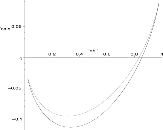
Figure 8: The energy curve ${\cal E}(\phi,\kappa_{0}(\phi))$ for $\epsilon=0.01$ and $c=16{\hat{g}}^{2}\epsilon=0.1$ is the lower one. The upper curve uses the linear interpolation for the matter$+$ghost energy as in Section 3. We see that the differences between the two treatments are quite mild. We have set $D=2$ for this plot.

We can analyze the solutions analytically in the limit $\epsilon\rightarrow 0$. Solutions with $\phi\neq 0,1$ in the limit are obtained by expanding $\kappa$ and $\kappa_{0}$:

$$\kappa\approx-{3D\sqrt{\epsilon\phi}\over\pi},\qquad\kappa_{0}\approx-{2{\hat{g}}\sqrt{\epsilon}(1-2\phi)\over\sqrt{\phi(1-\phi)}}.$$ (75)

The $\sqrt{\epsilon}$ cancels, and the equation for the minimum becomes

$${3D\sqrt{\phi}\over\pi}-{2{\hat{g}}(1-2\phi)\over\sqrt{\phi(1-\phi)}}=0.$$ (76)

The left side is plotted for various ${\hat{g}}$ values in Fig. 9. As already mentioned, the solutions all lie in the range $0\leq\phi\leq 1/2$.

Figure 9: The left side of Eq. (76), which determines the mean field at finite ${\hat{g}}$ for various couplings. Note that all solutions are in the range $0\leq\phi\leq 1/2$, with strong coupling corresponding to the upper end of this range. We have set $D=2$ in this plot.

Notice that Eq. (76) simplifies to a cubic equation for $\phi$ with coefficients linear in ${\hat{g}}^{2}$. Thus the solution $\phi({\hat{g}})$ as an analytic function of ${\hat{g}}$ will have branch points in the finite ${\hat{g}}^{2}$ complex plane, and so its Taylor expansion about ${\hat{g}}=0$ will have a finite radius of convergence as expected for the sum of planar diagrams [8]. By virtue of the identification of the string tension $T_{eff}(\phi)=1/\sqrt{\beta\phi}=m\sqrt{\epsilon}/(a\sqrt{\phi})$, we see that all solutions for ${\hat{g}}$ finite as $\epsilon\rightarrow 0$ correspond to zero string tension. In other words the system falls apart into a tensionless soup.

Next we analyze the case for $\phi$ near zero. We define a rescaled mean field by $\eta\equiv\phi/{\epsilon}$ and take $\epsilon\rightarrow 0$ at fixed $\eta$. Note that this is the combination that enters the effective string tension $T_{eff}=1/\sqrt{\beta\phi}=m/\sqrt{a^{2}\eta}$, so a solution with finite $\eta$ in the limit $\epsilon\rightarrow 0$ would indicate a finite non-zero effective string tension suggesting string formation. Then we find for the energy in this limit

$${\cal E}(\eta{\epsilon},\kappa) \approx \epsilon\left(\epsilon{2D\over\pi}\eta^{2}\arctan{1\over\sqrt{\eta}}-2\eta\sinh^{-1}{{\hat{g}}\over\sqrt{\eta}}-2\eta{{\hat{g}}\over{\hat{g}}+\sqrt{\eta+{\hat{g}}^{2}}}\right).$$ (77)

Applying the same limit to $\kappa$, we find

$$\kappa(\epsilon\eta)\approx-{D\epsilon\over\pi}\left(4\eta\arctan{1\over\sqrt{\eta}}-{\eta^{3/2}\over 1+\eta}\right),$$ (78)

and the slope of the energy is given by

$${d{\cal E}(\phi,\kappa_{0}(\phi))\over d\phi}=-\kappa(\phi)+\kappa_{0}(\phi).$$ (79)

The stationary points are of course the solutions of $\kappa=\kappa_{0}$. Since $\kappa=O(\epsilon)$, we can only get a solution at fixed $\eta$ if we also have ${\hat{g}}=O(\epsilon)$. Putting ${\hat{g}}=G\epsilon$, the stationarity condition reads

$${D\over\pi}\left(4\eta\arctan{1\over\sqrt{\eta}}-{\eta^{3/2}\over 1+\eta}\right)-{2G\over\sqrt{\eta}}=0.$$ (80)

It is clear from the fact that for any $G>0$, the left side goes to $-\infty$ ($+\infty$) when $\eta$ goes to 0 ($\infty$), that there is always a solution to this equation. Note incidentally that had we used (50) for the ghost$+$matter energy the first term on the left would have been replaced by $3D\sqrt{\eta}/\pi$, that is, by its asymptotic form at large $\eta$, and the same qualitative conclusion applies. But there are quantitative differences in the results. For comparison of the energy derived from (50) in the fixed $\eta$ regime with ${\hat{g}}=O(\epsilon)$ to (77) in the same regime we plot both energy curves for $G=1$ in Fig. 10.

Figure 10: Energy at fixed $\eta$ for $G={\hat{g}}/\epsilon=1$. The solid (lower) curve is from (77) and the dashed (higher) curve uses (50) for the matter$+$ghost energy. For this plot we set $D=2$.

Finally we note that for $G\ll 1$ or ${\hat{g}}\ll\epsilon$, there is a solution for $\eta\ll 1$ given by $\eta\approx(G/D)^{2/3}$, which corresponds to effective tension $T_{eff}\approx m(D/G)^{1/3}/a$. This limit corresponds to the regime of perturbation theory where the worldsheet fields in the bulk of the world sheet are constrained in terms of the fields on the boundaries.

5 Conclusions

In this article, we have presented a scheme for approximately summing Feynman graphs of arbitrary order. The scheme is an adaptation of the mean field method, widely used in many body physics and field theory, to the worldsheet representation of perturbation theory that we have developed earlier. For simplicity, we chose $\phi^{3}$ as a toy model for study, although we hope to apply the methods developed here to more realistic models, such as non-abelian gauge theories. The goal was to investigate under what circumstances string formation is possible in field theory. The worldsheet reformulation of field theory seems ideally suited to such an investigation; in particular, the field $\phi$, which naturally appears in this formulation and which roughly represents the density of propagating particles, is closely related to the string tension. A non-zero expectation value for this field signals formation of a string with finite tension.

The problem is to find a reliable way to compute this expectation value. In this article, we have used the mean field method as a possible approach to this problem. In this approach, the fields on the worldsheet are assigned various background expectation values, which are then calculated self consistently by minimizing the total energy of the system. In this fashion, one can find out whether the energetics can support a non-zero string tension. Unfortunately, there are many technical difficulties in carrying out this program. The biggest problem is connected with the delicate cancelation between the matter and ghost sectors, where two big numbers can cancel each other to give zero. Because of this, the results of any approximate treatment can be somewhat unstable. We try to bypass some of these problems by adopting a simple minded approach in the continuum version of the worldsheet in section 3. The calculation supports string formation in the intermediate and strong coupling regimes. In section 4, the mean field method is applied to the worldsheet lattice, where various details can be treated more exactly than in the continuum approach. There the mean field approximation was identified with a certain saddle-point evaluation of the worldsheet path integral. Despite its more solid starting point, this approach also suffers from possible ambiguities in the choice of zeroth order actions for the approximate evaluation. These ambiguities are partially resolved by choosing a zeroth order action that has a transparent formal continuum limit and agrees well with an exact calculation of the contribution of equally spaced solid lines in the zero coupling limit. The outcome of the lattice calculation, which also results in string formation in the strong coupling regime, is in qualitative agreement with the results of section 3, although there are some quantitative differences. The most notable of these is the $3/2$ power dependence of the matter energy on the field $\phi$ (Eq. (51)), as opposed to the linear dependence given by (28). We attribute this difference to the different ways of handling the matter-ghost cancelation mentioned earlier, and we are moderately encouraged that there is qualitative agreement. We also recall the point made in Section 3 that neither the continuum nor the lattice methods adequately treat the so-called small black regions. These correspond to fluctuations of the field $\phi$ over regions of the size of a small number of lattice sites. The mean field approximation, which at least in the leading order, treats $\phi$ as a constant over the whole worldsheet, neglects these fluctuations. There is indication, for example from the calculation of density of solid lines at the end of section 3, that these small black regions may play an important role in string formation. The identification made in Section 4 of the approximation with a saddle-point evaluation provides a useful setting to systematically explore the ramifications of these fluctuation effects.

Because of its various shortcomings mentioned above, we consider the dynamical calculation presented in this article as a promising initial attempt, not the final word. We hope that the line of approach developed here will stimulate further progress in this important problem of string formation in field theory.

Acknowledgments: We would like to thank Jeff Greensite, Rajeesh Gopakumar, Igor Klebanov, Anatoly Konechny, and Juan Maldacena for helpful conversations. CBT benefited from the hospitality of the Institute for advanced Study at Princeton and the Center for Theoretical Physics at MIT, where part of this work was done. This work was supported in part by the Monell Foundation, in part by the Department of Energy under Grant No. DE-FG02-97ER-41029 and Contract No. DE-AC03-76F00098, and in part by the National Science Foundation Grant PHY-0098840.

Appendix A Determinants

All of the Gaussian integrals we need in this paper are of the generic form

$${\cal I} = \int D{q}\exp\left\{-\sum_{i,j}\left[A{({q}_{i}^{j}-{q}_{i}^{j-1})^{2}}+B{({q}_{i+1}^{j}-{q}_{i}^{j})^{2}}\right]\right\}$$ (81)

These integrals can be done exactly using the methods of [4]. For simplicity we impose periodic boundary conditions in $\sigma$ and Dirichlet conditions in $\tau$, which describes a closed string moving in a background of Ising spins.

The eigenvalues of the bilinear forms in the exponent are well-known, so the integral which is proportional to one over the square root of the determinant of the bilinear form can be written as a double product, so we find for two bosonic variables:

$$\hskip-25.6073pt{\cal I}^{2}=\left({\pi\over A}\right)^{MN}\prod_{n=1}^{N}\prod_{l=0}^{M-1}\left(4\sin^{2}{n\pi\over 2(N+1)}+4{B\over A}\sin^{2}{l\pi\over M}\right)^{-1}$$ (82)

The analogous ghost integrals will be the reciprocal of this expression (with of course different values for $A,B$. We list some infinite products from [4]:

$$\prod_{n=1}^{N}\left(4\sin^{2}\left({n\pi\over 2(N+1)}\right)-z\right) = {\sin(N+1)\kappa\over\sin\kappa},\qquad z\equiv 4\sin^{2}{\kappa\over 2}$$ (83)

$$\prod_{l=1}^{M-1}\left(4\sin^{2}{l\pi\over M}-z\right) = {\sin^{2}M\lambda\over\sin^{2}\lambda},\qquad z\equiv 4\sin^{2}\lambda$$ (84)

$$\prod_{l=1}^{M-1}\left(2\sin{l\pi\over M}\right)=M,\qquad \qquad\prod_{n=1}^{N}\left(2\sin{n\pi\over 2(N+1)}\right)=\sqrt{N+1},$$ (85)

the last line being just the case $z=0$ of the first two. Using these products, we then find

$${\cal I}^{2} = {1\over{N+1}}\left({\pi\over A}\right)^{MN}\prod_{l=1}^{M-1}\left({\sinh(N+1)\xi_{l}\over\sinh\xi_{l}}\right)^{-1},\qquad\sinh^{2}{\xi_{l}\over 2}={B\over A}\sin^{2}{l\pi\over M}$$ (86)

The ground state energy associated with this system of two bosonic variables can be read off by identifying the coefficient of $-N$ in $\ln{\cal M}$ as $N\rightarrow\infty$:

$$aE_{G} = -M\ln{2\pi a\over\beta m\phi^{2}}+2\sum_{l=1}^{M-1}\sinh^{-1}\left({\sqrt{\epsilon}\over{\phi}}\sin{l\pi\over M}\right)$$ (87)

where we note that $\sinh^{-1}(z)=\ln(z+\sqrt{1+z^{2}})$. So far everything is exact. Now let’s consider the continuum limit, $M\rightarrow\infty$. Note that since $a,m\rightarrow 0$ together in the continuum limit, it is valid to keep $a/m$ fixed. We also keep $A,B$ fixed. The bulk contributions to this limit are straightforward:

$${aE_{G}\over M} \rightarrow 2\int_{0}^{1}dx\sinh^{-1}\left({\sqrt{B}\over\sqrt{A}}\sin{x\pi}\right)-\ln{\pi\over A}={4\over\pi}{\rm Re}\left\{i{\rm Li}_{2}\left({\sqrt{B}\over i\sqrt{A}}\right)\right\}-\ln{\pi\over A}$$ (88)

We note the appearance of the dilogarithm or Spence function ${\rm Li}_{2}(x)={\rm dilog}(1-x)=\sum_{k=1}^{\infty}{x^{n}/n^{2}}$.

Appendix B Slowly Varying Mean Fields

The identification of the mean field approximation with a saddle point approximation to the path integral, enables an easy extension to slowly varying fields. Indeed we have already seen in the footnote to Eq. 60, the relatively simple extension of the effective action for ghost$+$ matter fields to slowly varying fields. Here we sketch the corresponding extension for the spin system sum. This will give dynamical terms to the mean field.

We first write out the saddle point equation for general (non-uniform) $\phi,\lambda$.

$$\phi_{kl}={\sum_{s_{i}^{j}=\pm 1}P_{k}^{l}\left({\hat{g}}^{\prime}\right)^{(1-s_{i}^{j}s_{i}^{j-1})/2}e^{{-i\sum_{ij}\lambda_{ij}P_{i}^{j}}}\over\sum_{s_{i}^{j}=\pm 1}\left({\hat{g}}^{\prime}\right)^{(1-s_{i}^{j}s_{i}^{j-1})/2}e^{{-i\sum_{ij}\lambda_{ij}P_{i}^{j}}}}.$$ (89)

This equation implicitly determines $\lambda_{ij}(\phi)$ as a function of all the $\phi_{ij}$. The equation is intractable for general $\phi_{ij}$, but we have seen in the main text how to explicitly solve the equation for uniform $\phi$, obtaining $\lambda_{ij}=i\kappa_{0}(\phi)$. We can get a perturbative solution for slowly varying $\phi_{ij}=\phi_{0}+\delta\phi_{ij}$. Actually, rather than $\lambda$ itself, we are more interested in expanding the effective action

$$W_{s}(\phi,\lambda(\phi)) = \sum_{ij}\phi_{ij}\lambda_{ij}-f(\lambda)$$ (90)

$$e^{-if(\lambda)} \equiv \sum_{s_{i}^{j}=\pm 1}\left({\hat{g}}^{\prime}\right)^{(1-s_{i}^{j}s_{i}^{j-1})/2}e^{{-i\sum_{ij}\lambda_{ij}P_{i}^{j}}}$$ (91)

about $\phi_{0}$. To expand to second order in $\delta\phi$, we only need to compute first and second derivatives of $W_{s}$, which by virtue of the fact that $W_{s}$ is a Legendre transform, are simply:

$${\partial W_{s}\over\partial\phi_{ij}} = \lambda_{ij}(\phi_{0})$$ (92)

$${\partial^{2}W_{s}\over\partial\phi_{mn}\partial\phi_{ij}} = {\partial\lambda_{ij}\over\partial\phi_{mn}}\bigg{|}_{\phi=\phi_{0}}.$$ (93)

Then the expansion to quadratic order reads

$$W_{s}(\phi,\lambda(\phi))=W_{s}(\phi_{0},\lambda(\phi_{0}))+\sum_{ij}\delta\phi_{ij}i\kappa_{0}(\phi_{0})+{1\over 2}\sum_{ij,mn}\delta\phi_{ij}\delta\phi_{mn}{\partial\lambda_{ij}\over\partial\phi_{mn}}\bigg{|}_{\phi=\phi_{0}}+O(\delta\phi^{3}).$$ (94)

The matrix $\partial\lambda/\partial\phi$ is the inverse of the matrix $\partial\phi/\partial\lambda$, which can be related to spin correlators by

$${\partial\phi_{ij}\over\partial\lambda_{mn}} = -i[\langle P_{i}^{j}P_{m}^{n}\rangle-\langle P_{i}^{j}\rangle\langle P_{m}^{n}\rangle]$$ (95)

$$\langle\Omega\rangle \equiv {\sum_{s_{i}^{j}=\pm 1}\Omega\left({\hat{g}}^{\prime}\right)^{(1-s_{i}^{j}s_{i}^{j-1})/2}e^{{\sum_{ij}\kappa_{0}(\phi_{0})P_{i}^{j}}}\over\sum_{s_{i}^{j}=\pm 1}\left({\hat{g}}^{\prime}\right)^{(1-s_{i}^{j}s_{i}^{j-1})/2}e^{{\sum_{ij}\kappa_{0}(\phi_{0})P_{i}^{j}}}}.$$ (96)

Since these spin correlators are all in the presence of a uniform background field $\lambda$, they may be explicitly evaluated in terms of the eigenvalues of the spin transfer matrix introduced in Section 4.

$$\langle P_{i}^{j}P_{m}^{n}\rangle=\langle P_{i}^{j}\rangle\langle P_{m}^{n}\rangle+\delta_{im}\left({t_{-}\over t_{+}}\right)^{|j-n|}{{\hat{g}}^{\prime 2}\over 4({\hat{g}}^{\prime 2}+\sinh^{2}(\kappa_{0}/2))}$$ (97)

so that

$${\partial\phi_{ij}\over\partial\lambda_{mn}} = -i\delta_{im}\left({t_{-}\over t_{+}}\right)^{|j-n|}{{\hat{g}}^{\prime 2}\over 4({\hat{g}}^{\prime 2}+\sinh^{2}(\kappa_{0}/2))}.$$ (98)

The matrix $M_{jn}=\rho^{|j-n|}$ can be inverted by defining $w_{j}=\sum_{n}\rho^{|j-n|}v_{n}$ and proving the recursion relation

$$w_{j+1}+w_{j-1}=(\rho+1/\rho)w_{j}+(\rho-1/\rho)v_{j},$$ (99)

from which it follows that

$$(M^{-1})_{jn} = {\rho\over\rho^{2}-1}(\delta_{j+1,n}+\delta_{j-1,n}-2\delta_{jn})-{\rho-1\over\rho+1}\delta_{jn}$$ (100)

$$= -{(1-{\hat{g}}^{\prime 2})(\delta_{j+1,n}+\delta_{j-1,n}-2\delta_{jn})\over 4\cosh(\kappa/2)\sqrt{{\hat{g}}^{\prime 2}+\sinh^{2}(\kappa/2)}}+\delta_{jn}{\sqrt{{\hat{g}}^{\prime 2}+\sinh^{2}(\kappa/2)}\over\cosh(\kappa/2)}.$$

Plugging these results into the quadratic approximation to the spin system effective action then gives

$$iW_{s}(\phi,\lambda(\phi)) \approx iW_{s}(\phi_{0},i\kappa_{0}(\phi_{0}))-\sum_{ij}\delta\phi_{ij}\kappa_{0}(\phi_{0})-{1\over 2}\sum_{ij}\left[Z(\delta\phi_{ij}-\delta\phi_{i,j-1})^{2}+\mu^{2}\delta\phi^{2}_{ij}\right]$$ (101)

$$Z \equiv {(1-{\hat{g}}^{\prime 2})\sqrt{{\hat{g}}^{\prime 2}+\sinh^{2}(\kappa/2)}\over{\hat{g}}^{\prime 2}\cosh(\kappa/2)},\qquad\mu^{2}\equiv 4{({\hat{g}}^{\prime 2}+\sinh^{2}(\kappa/2))^{3/2}\over{\hat{g}}^{\prime 2}\cosh(\kappa/2)}.$$ (102)

This result gives the spin system effective action for $\phi_{ij}=\phi_{0}+\delta\phi_{ij}$ to quadratic order in $\delta\phi$. Formally $\phi_{0}$ can be chosen to be anything, but to minimize corrections to the slowly varying mean field approximation, it should be chosen so that $\sum_{ij}\delta\phi_{ij}=0$. In the uniform mean field approximation studied in the main text, this means simply $\phi_{ij}=\phi=\phi_{0}$.

It is instructive to combine the work of this appendix with that in the footnote to Eq. 60 to give the formal continuum limit of the total effective action to order $\delta\phi^{2}$:

$$S = -iW_{s}(\phi_{0},i\kappa_{0}(\phi_{0}))+\int d\tau d\sigma\left({1\over 2}{\bf q}^{\prime 2}+{a^{2}\phi\over 2m^{2}\epsilon}{\dot{\bf q}}^{2}-(1-\phi^{2})^{2}b^{\prime}c^{\prime}-{a^{2}\phi\over m^{2}\epsilon}{\dot{b}}{\dot{c}}\right.$$ (103)

$$\left.\hskip 85.35826pt-{1\over 2}(\phi^{\prime\prime}+2\phi^{\prime 2})bc+{aZ\over 2m}{\dot{\phi}}^{2}+{\mu^{2}\over 2am}(\phi-\phi_{0})^{2}\right)+O(\phi-\phi_{0})^{3}.$$

This equation expresses the mean field dynamics for our system in a form tantalizingly close to the outcome of the Maldacena conjecture [2]. The mean field has emerged as a dynamical Liouville-like worldsheet field that enters the worldsheet action in a way strongly reminiscent of the way the radial AdS coordinate enters the worldsheet action for the “string” description of ${\cal N}=4$ super-Yang-Mills theory.

References

- [1] K. Bardakci and C. B. Thorn, Nucl. Phys. B 626 (2002) 287 [arXiv:hep-th/0110301].
- [2] J. M. Maldacena, Adv. Theor. Math. Phys. 2 (1998) 231-252, hep-th/9711200.
- [3] C. B. Thorn, arXiv:hep-th/0203167.
- [4] R. Giles and C. B. Thorn, Phys. Rev. D16 (1977) 366.
- [5] P. Orland, Nucl. Phys. B 278 (1986) 790.
- [6] S. Dalley and I. R. Klebanov, Phys. Lett. B 298 (1993) 79 [arXiv:hep-th/9207065].
- [7] J. Greensite and M. B. Halpern, Nucl. Phys. B 242 (1984) 167.
- [8] G. ’t Hooft, Phys. Lett. B 119 (1982) 369, Commun. Math. Phys. 88 (1983) 1.