A new analytic approach to physical observables in QCD

Abstract:

An analytic ghost-free model for the QCD running coupling $\alpha(Q^{2})$ is proposed. It is constructed from a more general approach we developed particularly for investigating physical observables of the type $F(Q^{2})$ in regions that are inaccessible to perturbative methods of quantum field theory. This approach directly links the infrared (IR) and the ultraviolet(UV) regions together under the causal analyticity requirement in the complex $Q^{2}-$plane. Due to the inclusion of crucial non-perturbative effects, the running coupling in our model not only excludes unphysical singularities but also freezes to a finite value at the IR limit $Q^{2}=0$. This makes it consistent with a popular phenomenological hypothesis, namely the IR freezing phenomenon. Applying this model to compute the Gluon condensate, we obtain a result that is in good agreement with the most recent phenomenological estimate. Having calculated the $\beta-$function corresponding to our QCD coupling constant, we find that it behaves qualitatively like its perturbative counterpart, when calculated beyond the leading order and with a number of quark flavours allowing for the occurrence of IR fixed points.

1 Introduction

A fundamental problem in the theory of particle physics lies in the description of hadron interactions in the infrared region. The property of asymptotic freedom [1] in QCD allows us to investigate the interactions of quarks and gluons at short distances using the standard perturbation theory. However, there is a number of phenomena whose description is intractable in perturbation theory, for example quark confinement and gluon and quark condensates. Hence, the search for calculational techniques that go beyond conventional perturbation theory remains essential (not only in QCD but in other field theories as well).

In standard perturbative QCD, for any number of quark flavours $n_{f}$, the running coupling constant (to leading order):

$$\alpha^{(1)}_{\mathrm{PT}}(Q^{2})=\frac{4\pi}{\beta_{0}}\,\frac{1}{\ln(Q^{2}/\Lambda^{2})}\qquad\textrm{with}\qquad\beta_{0}=11-\frac{2}{3}n_{f}\,,$$ (1)

diverges at a small mass scale $Q=\Lambda$, creating the so-called Landau ghost-pole problem. Taking next loop corrections into account does not alter the essence, and leads only to additional branch cuts along the positive real axis $\mathrm{Re}\{Q^{2}\}>0$. This problem prevents the use of perturbative expansion at small momentum transfers $Q\thicksim\Lambda$ and, in addition, generates infrared (IR) renormalon singularities on the positive real axis of the Borel parameter, destroying attempts to sum up the perturbative series [2, 3, 4, 5]. Generally speaking, as $Q^{2}$ comes below or near $\Lambda^{2}$ , non-perturbative effects become the most dominant and the perturbative expansion becomes useless.

Another indication that the perturbative formalism is incomplete, and cannot describe the low energy physics unless it is supplemented by non-perturbative corrections, comes from considering its analyticity structure in the complex $Q^{2}$-plane [6]; the upshot being that any QCD observable, which depends on a spacelike momentum variable $Q^{2}$, is expected to be an analytic function of $Q^{2}$ in the entire complex plane except the negative real (timelike) axis. Singularities on the timelike axis are meaningful since they correspond to production of on-shell particles, while their existence on the spacelike axis is non-physical as this would violate causality (i.e. causal analyticity structure) [6, 7]. For example, if a generic QCD observable were calculated to leading order, it would depend on $\alpha^{(1)}_{\mathrm{PT}}(Q^{2})$, inheriting the Landau-singularity at $Q^{2}=\Lambda^{2}$. This singularity is obviously non-physical as it lies on the positive real axis $\mathrm{Re}\{Q^{2}\}>0$. From this point of view, causality constrains the $Q^{2}-$dependence of physical observables, and is consistent with perturbative results only if the coupling constant is non-singular on the entire $Q^{2}$-plane with the exception of the timelike axis $\mathrm{Re}\{Q^{2}\}<0$.

A small number of models for the QCD running coupling $\alpha(Q^{2})$ have been proposed [5, 7, 8, 9, 10] to comply with the causality condition, i.e. the requirement of analyticity in $Q^{2}$. However, the issue of which of these is the most realistic is still a moot point. Quite recently, a good attempt has been made, by Shirkov and Solovtsov [8], to devise a model for the running coupling that is completely free of singularities in the IR region. In this approach, the analytic running coupling is defined via the so-called Källén-Lehmann spectral representation as:

$$\alpha_{\mathrm{an}}^{(n)}(Q^{2})=4\,\int^{\infty}_{0}\frac{\rho^{(n)}(x)}{(x+Q^{2}-i\epsilon)}\,dx\,,$$ (2)

with the $n$-loop spectral density $\rho^{(n)}(x)$ given by

$$\rho^{(n)}(x)=\frac{1}{4\pi}\mathrm{Im}\{\alpha^{(n)}_{\mathrm{PT}}(-x-i\epsilon)\}\,,$$ (3)

where $\alpha^{(n)}_{\mathrm{PT}}$ is the coupling constant obtained from perturbation theory (PT) at the n-loop approximation. To leading order, the corresponding spectral density reads as:

$$\rho^{(1)}(x)=\frac{\pi}{\beta_{0}}\,\frac{1}{[\pi^{2}+\ln^{2}(x/\Lambda^{2})]}\,.$$ (4)

Inserting this into (2) gives the one-loop analytic spacelike coupling constant:

$$\alpha^{(1)}_{\mathrm{an}}(Q^{2})=\frac{4\pi}{\beta_{0}}\,\bigg{[}\frac{1}{\ln(Q^{2}/\Lambda^{2})}+\frac{1}{1-Q^{2}/\Lambda^{2}}\bigg{]}\,.$$ (5)

This expression is consistent with the causality condition. The first term on the right-hand side of (5) preserves the standard UV behaviour whereas the second term compensates for the ghost-pole at $Q^{2}=\Lambda^{2}$. Obviously the second term in (5) comes from the spectral representation and enforces the required analytic properties. Thus, it is essentially non-perturbative. However, as mentioned in Ref.[7], as this term introduces a $1/Q^{2}$ correction to $\alpha^{(1)}_{\mathrm{PT}}(Q^{2})$ at large $Q^{2}$ it would make (5) unsuitable as an input quantity for observables that are proportional to the running coupling (in leading order) but are not expected to have $1/Q^{2}$ corrections (such as the $e^{+}e^{-}$ total cross section) because in such cases the unwanted $1/Q^{2}$ correction would have to be artificially cancelled. By construction, (5) does not include any adjustable parameters other than the QCD characteristic mass scale $\Lambda$. Thus, one might prefer to have a model with free extra parameters that would allow for the fitting of the coupling to lower energy experimental data and hence further improve perturbative results at low $Q^{2}$. An example of a model of this type is suggested in Ref.[9], where the one-loop coupling constant assumes the form:

$$\alpha^{(1)}(Q^{2})=\frac{4\pi}{\beta_{0}}\,\bigg{[}\frac{Q^{2\,p}/\Lambda^{2\,p}}{Q^{2\,p}/\Lambda^{2\,p}+C_{p}}\bigg{]}\;\frac{p}{\ln(Q^{2\,p}/\Lambda^{2\,p}+C_{p})}\,,$$ (6)

with $C_{p}\geq 1$. For $Q^{2}\gg\sqrt[p]{C_{p}}\,\Lambda^{2}$, this expression recovers the perturbative asymptotic form (1). Although (6) is a ghost-pole free expression, being analytic for all $Q^{2}\in[0,\infty)$ , it contains unphysical singularities on the complex $Q^{2}-$plane (for all $p>1$) and hence does not comply with causality. A careful analytic study of non-perturbative effects is always important in QCD because it provides more reliable and useful information about the IR region, which is inaccessible to perturbative methods.

The main purpose of this paper is to construct a new analytic approach based on a different and more general methodology to that of Shirkov and Solovtsov, which improves perturbative results outside the asymptotic domain and respects the causal analyticity structure in, at least, the right half of the complex $Q^{2}-$plane. Having achieved this, we apply our method to the QCD coupling constant to solve the Landau ghost-pole problem without altering the correct perturbative behaviour in the UV region. Then, we show that the resultant QCD coupling in this way freezes to a finite value at the origin (i.e. $Q^{2}=0$), supporting the IR freezing idea which has long been a popular and successful phenomenological hypothesis [11, 12]. Moreover, from the viewpoint of the new background field formalism [3, 4] our approach provides better estimates for the IR fixed points than that of Shirkov and Solovtso.

The layout of this paper is as follows: In section 2, we discuss our analyticization procedure on general grounds, proposing a new integral representation for physical observables that depend on a spacelike momentum variable (squared) $Q^{2}$. In the next section, we present a full derivation of our analytic coupling constant, giving a new expression that depends on a free extra parameters $\lambda_{e}$ which can be used to tune the coupling to lower energy experimental data. An approximation scheme for estimating the value of $\lambda_{e}$ is included in section 4. In section 5, we carry out a comprehensive comparison between the predictions in our approach and those estimated by other theoretical methods, which include conventional perturbation theory, optimized perturbation theory, background field formalism and the analytic approach of Shirkov and Solovtsov. In this section, we test our model on a fit-invariant IR characteristic integral extracted from jet physics data. For further applications, we use our analytic coupling constant in the instanton density derived from the dilute instanton-gas approximation to estimate the gluon condensate. Then, we show that the result obtained is in good agreement with the value phenomenologically estimated from the QCD sum rules. Finally, we end this section by calculating the $\beta-$function which corresponds to our analytic coupling constant and compare its behaviour with the perturbative counterpart. We further show that the $\beta-$function in our approach and that in higher-loop order perturbation theory behave qualitatively the same in the range of $n_{f}-$values that allows perturbation theory to obtain IR fixed points. The last section is devoted to our conclusions.

2 Analyticization Procedure

We will illustrate our method with the following pedagogical example. Consider a physical observable $F$ depending on a positive variable $q$ with the dimensions of energy squared. Then, it follows from the principle of causality, mentioned earlier, that $F(q)$ can be analytically continued to the complex plane excluding the negative real axis. As we shall show, this will allow us to reconstruct $F(q)$ from its high energy behaviour by using the contour integral representation:

$$\bar{F}(q,\lambda)=\frac{1}{2\pi i}\,\int_{C_{UV}}\,\,\frac{{\mathrm{e}}^{\lambda(k-q)}}{k-q}\;\,F(k)\>dk\,,$$ (7)

where $C_{UV}$ is a very large incomplete circle, in the complex $k-$plane, with radius $R_{UV}$ and centre at the origin, beginning just below the negative real axis and ending just above and $q\in\{\;\textrm{Re}\;k\,:\>\>0<\textrm{Re}\;k<R_{UV}\}$ as depicted in Fig.(1).

Figure 1: Sketch of the integration contour $C_{UV}$ in the cut complex $k-$plane. The thick line represents a branch cut and the cross indicates the location of $q$.

We will show that $F(q)$ is recovered as the limit as $\lambda\rightarrow\infty$ of $\bar{F}(q,\lambda)$, and this depends mainly on the ultraviolet behaviour of $F(q)$ when we take $R_{UV}$ to be sufficiently large. In order to achieve this goal, we exploit the analyticity of $F(k)$ in the complex $k$-plane, using Cauchy’s theorem to replace the UV-boundary $C_{UV}$ in (7) with a small circle $C_{0}$ around $q$ and a keyhole shaped contour $C_{k}$, depicted in Fig.(2), surrounding the cut and not connected to $C_{0}$.

Figure 2: Sketch of the keyhole shaped contour $C_{k}$. The thick line represents the branch cut $\textrm{Re}\;k\leq 0$. Here, $\epsilon$ is an infinitesimally small radius and $\theta\in(-\pi,\pi]$.

For this deformed contour, Cauchy’s integral formula over the circle $C_{0}$ yields $F(q)$ which together with the integral over the keyhole contour $C_{k}$ transforms (7) into the form:

$$\bar{F}(q,\lambda)=\,F(q)\,+\,I_{C_{k}},$$ (8)

where

$$I_{C_{k}}=\frac{1}{2\pi i}\,\int_{C_{k}}\,\,\frac{{\mathrm{e}}^{\lambda(k-q)}}{k-q}\,\,F(k)\,dk.$$ (9)

If we restrict attention to those functions $F(k)$ which are finite on the line of discontinuity along the negative real $k$-axis, e.g. $F(k)\propto\sqrt{k}$, then we can write $I_{C_{k}}$ more explicitly as:

$$I_{C_{k}}=\int^{R_{UV}}_{\epsilon}\,\,\frac{{\mathrm{e}}^{-\lambda(r+q)}}{r+q}\;\;\Delta(r)\,dr\;+\;\frac{\epsilon\,{\mathrm{e}}^{-\lambda q}}{2\pi}\,\int^{\pi}_{-\pi}{\mathrm{e}}^{\lambda\epsilon\cos(\theta)}\,\;\textrm{f}_{\epsilon}(\theta,q)\;d\theta,$$ (10)

with

$$\Delta(r)=\frac{1}{2\pi i}\;[\;F(r\,{\mathrm{e}}^{i\pi})\,-\,F(r\,{\mathrm{e}}^{-i\pi})\;]\,,$$ (11)

and

$$\textrm{f}_{\epsilon}(\theta,q)=\frac{1}{2}\,\Bigg{[}\,\frac{{\mathrm{e}}^{i\lambda\epsilon\sin(\theta)}\;F(\epsilon{\mathrm{e}}^{i\theta})}{\epsilon-q\;{\mathrm{e}}^{-i\theta}}+\frac{{\mathrm{e}}^{-i\lambda\epsilon\sin(\theta)}\;F(\epsilon{\mathrm{e}}^{-i\theta})}{\epsilon-q\;{\mathrm{e}}^{i\theta}}\,\Bigg{]}.$$ (12)

Owing to the discontinuity of $F(k)$ across the cut, given by $2\pi i\,\Delta(|k|)\,$, the sum of the line integrals on each side of the branch cut does not cancel. Since the region of analyticity of $F(k)$:

$$S_{an}=\{k=r\,{\mathrm{e}}^{i\theta}:\,r>0\,,\,-\pi<\theta\leq\pi\},$$ (13)

includes a portion of the real axis on which $F(k)$ is real, it follows that $F(k)$ satisfies the Schwarz Reflection Principle [14]:

$$F^{*}(k)=F({k}^{*}).$$ (14)

This allows us to rewrite $\Delta(r)$ and $\textrm{f}_{\epsilon}(\theta)$ in the more compact forms:

$$\Delta(r)=\frac{1}{\pi}\;\textrm{Im}\Big{\{}\;F(r\,{\mathrm{e}}^{i\pi})\;\Big{\}}\,,$$ (15)

and

$$\textrm{f}_{\epsilon}(\theta,q)=\textrm{Re}\,\Bigg{\{}\,\frac{{\mathrm{e}}^{i\lambda\epsilon\sin(\theta)}\;F(\epsilon\,{\mathrm{e}}^{i\theta})}{\epsilon-q\;{\mathrm{e}}^{-i\theta}}\,\Bigg{\}},$$ (16)

which imply that $I_{C_{k}}$ is a purely real quantity as it should be.

In the following, we will investigate the behaviour of $I_{C_{k}}$ at sufficiently large values of $\lambda$. Since $F(r\,{\mathrm{e}}^{i\theta})$ is assumed finite throughout the whole region $S_{an}$, we take its magnitude to be bounded on the infinitesimal circle $|k|=\epsilon$, see Fig.(2), such that:

$$|F(\epsilon\,{\mathrm{e}}^{i\theta})|\leq M\,,\qquad\textrm{for}\quad-\pi<\theta\leq\pi\,,$$ (17)

where $M$ is a positive constant which may depend on $\epsilon$. Using this to estimate the upper bound of the second term in (10), we find that:

$$\frac{\epsilon\,{\mathrm{e}}^{-\lambda q}}{2\pi}\,\Bigg{|}\int^{\pi}_{-\pi}{\mathrm{e}}^{\lambda\epsilon\cos(\theta)}\,\;\textrm{f}_{\epsilon}(\theta,q)\;d\theta\Bigg{|}\leq\frac{\epsilon\,M\,{\mathrm{e}}^{-\lambda(q-\epsilon)}}{q-\epsilon}.$$ (18)

If we consider only those functions $F$ for which $M$ can be chosen such that $\displaystyle{\lim_{\epsilon\rightarrow 0}}\;\epsilon M=0$ then the second term in (10) will vanish in this limit and accordingly $I_{C_{k}}$ reduces to the form:

$$I_{C_{k}}(q,\lambda)=\int^{R_{UV}}_{0}\,\,\frac{{\mathrm{e}}^{-\lambda(r+q)}}{r+q}\;\,\Delta(r)\;dr,\qquad q>0\,,$$ (19)

which is more suitable for further calculations. For the case under consideration, since $\Delta(r)$ has an upper bound $N>0$, i.e. $|\Delta(r)|\leq N\,$, in the interval $0\leq r\leq R_{UV}$, we deduce that:

$$|I_{C_{k}}|\leq N\;\frac{{\mathrm{e}}^{-\lambda q}}{\lambda q}\;\left(1-{\mathrm{e}}^{-\lambda R_{UV}}\right).$$ (20)

So for large values of $\lambda$, the function $I_{C_{k}}(q,\lambda)$ decays rapidly to zero, and:

$$\lim_{\lambda\rightarrow\infty}I_{C_{k}}(q,\lambda)=0\,.$$ (21)

In general, (21) remains true even if the finiteness restriction on $F(k)$ along the negative real $k$-axis, together with the constraint $\displaystyle{\lim_{\epsilon\rightarrow 0}\epsilon M=0}$, is not fulfilled. For example, if $F(k)$ has a finite number of singularities on the negative real axis then we can avoid these points by keeping the two edges of the keyhole contour $C_{k}$ a small distance $\delta$ away from the cut which they surround. In this way, we can rewrite (9) as:

$$I_{C_{k}}=\int^{R_{UV}}_{\epsilon^{\prime}}{\mathrm{e}}^{-\lambda(x+q)}\;\;\textrm{g}(x,q,\lambda)\,dx\,+\,\frac{\epsilon\,{\mathrm{e}}^{-\lambda q}}{2\pi}\,\int^{\pi-\eta}_{-\pi+\eta}{\mathrm{e}}^{\lambda\epsilon\cos(\theta)}\,\;\textrm{f}_{\epsilon}(\theta,q)\;d\theta,$$ (22)

where $\epsilon^{\prime}=\sqrt{\epsilon^{2}-\delta^{2}}\;$ with $\epsilon>\delta\,$, $\,\eta=\arctan{(\delta/\epsilon^{\prime})}$ and:

$$\textrm{g}(x,q,\lambda)=\frac{1}{\pi}\;\mathrm{Im}\,\Big{\{}\,\frac{\mathrm{e}^{i\lambda\,\delta}}{x+q-i\delta}\;\;F(-x+i\delta)\,\Big{\}}\,.$$ (23)

Since $F$ is bounded on the contour $C_{k}\,$, we have:

$$|I_{C_{k}}|\leq\,\frac{N^{\prime}}{\pi}\;\frac{{\mathrm{e}}^{-\lambda q}}{\lambda(q+\epsilon^{\prime}-\delta)}\;\Big{[}{\mathrm{e}}^{-\lambda\epsilon^{\prime}}-{\mathrm{e}}^{-\lambda R_{UV}}\Big{]}\;+\;\frac{\epsilon\,M\,(\pi-\eta)}{\pi}\;\;\frac{{\mathrm{e}}^{-\lambda(q-\epsilon)}}{q-\epsilon}\,,$$ (24)

where $N^{\prime}$ is the upper bound of $F(-x+i\delta)$ for all $x\in[\epsilon^{\prime},R_{UV}]\,$. As both $N^{\prime}$ and $M$ are $\lambda$-independent, in the limit as $\lambda\to\infty$ we obtain (21) as claimed above. So, by taking the limit as $\lambda\to\infty$ in (8) we deduce from (21) that:

$$\lim_{\lambda\rightarrow\infty}\bar{F}(q,\lambda)=F(q)\,.$$ (25)

To have some notion of the functional dependence of $\bar{F}(q,\lambda)$ on $\lambda$, for a fixed $q>0$, consider the simple example where the imaginary part of $F(k)$ assumes a constant value $\mu_{0}$ along the upper edge of the cut, e.g. $F(k)\propto\ln k$. In this case, we have $\Delta(r)=\mu_{0}/\pi$ and a straightforward integration of (19) yields:

$$I_{C_{k}}(q,\lambda)=\,\frac{\mu_{0}}{\pi}\;\Big{[}E_{1}(\lambda q)-E_{1}(\lambda(q+R_{UV}))\Big{]}\,,$$ (26)

where $E_{1}(x)$ denotes the exponential integral function [15] defined by:

$$E_{1}(x)=\int^{\infty}_{x}\frac{{\mathrm{e}}^{-t}}{t}\>dt=-\gamma-\ln(x)-\sum_{n=1}^{\infty}\frac{(-1)^{n}}{n!\,n}\;x^{n}\qquad\textrm{for}\>\>\>x>0\,,$$ (27)

here $\gamma\cong 0.577215$ is the well-known Euler’s constant. By inserting (26) into (8) and sending $R_{UV}\to\infty$, we immediately arrive at an explicit solution:

$$\bar{F}(q,\lambda)=F(q)+\,\frac{\mu_{0}}{\pi}\;E_{1}(\lambda q)\,.$$ (28)

As illustrated by the graph in Fig.(3), the variation of $\bar{F}(q,\lambda)$ with respect to $\lambda$ depends largely on both the sign of $\mu_{0}$ and the behaviour of $E_{1}(\lambda q)$. With increasing $\lambda$, we see that $\bar{F}(q,\lambda)$ evolves from $-\infty$, for $\mu_{0}<0$, or $+\infty$, for $\mu_{0}>0$, in a continuous progression until it settles down to the value $F(q)$ at large values of $\lambda$. Moreover, we discover from (28) that $\bar{F}(q,\lambda)$ converges to $F(q)$ faster as $q$ increases.

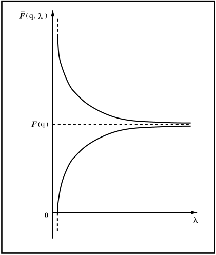
Figure 3: The variation of $\bar{F}(q,\lambda)$ versus $\lambda$ at a fixed value $q$ . The lower and the upper curves describe the cases in which $\mu_{0}<0$ and $\mu_{0}>0$, respectively. The dashed line represents $F(q)$.

To summarise, by exploiting the analyticity of $F(k)$ in (7), we can obtain $F(q)$ as $\lim_{\lambda\rightarrow\infty}\bar{F}(q,\lambda)$, and if we take the radius $R_{UV}$ of the contour $C_{UV}$ to be sufficiently large the integrand depends on the large $q$ behaviour of $F$. So far, our consideration has been restricted to the case in which $F(q)$, as a true function for the observable in question, complies with the principle of causality. In practice, however, we do not know the function $F(q)$ exactly, even for large $q$, but for a theory with asymptotic freedom we can approximate the large $q$ behaviour of $F(q)$ using perturbation theory for $q$ in some high energy domain $D_{PT}$ so that $F_{PT}(q)\cong F(q)$ for $q\in D_{PT}$. Thus, for large enough $R_{UV}$, we can safely use $F_{PT}(k)$ as a reasonable substitute for $F(k)$ in our contour integral (7), where now $k$ is any point on $C_{UV}$. This gives the approximation $\bar{F}_{PT}(q,\lambda)\approx\bar{F}(q,\lambda)$, but taking $\lambda$ to infinity in this would simply reproduce the perturbative estimate for $F(q)$, leading to nothing new. Now $F_{PT}(q)$, as a perturbatively calculated quantity, often suffers from a serious defect by having singularities in the complex plane away from the negative real axis. Good examples of this are the effective coupling constant and the running mass in perturbative QCD. These extra singularities are unphysical and do not exist in the true function $F(q)$. Hence, they should be eliminated in our approximation in order to reinstate causality. So, if instead of using the limiting value of $\bar{F}_{PT}(q,\lambda)$ we were to use a finite value of $\lambda$, say $\lambda_{0}$, then we might have an expression in which these unphysical singularities are absent and we will give an example in which this happens. Furthermore, taking a finite value of $\lambda$ in $\bar{F}_{PT}(q,\lambda)$ can give an improvement over the perturbative estimate in favourable circumstances for the following reason: Viewed as a function of $\lambda$ with $q$ held fixed, $\bar{F}_{PT}(q,\lambda)$ is a better estimate of the true function $\bar{F}(q,\lambda)$ for small $\lambda$ than it is for large $\lambda$ since if we scale the integration variable in (7) then:

$$\bar{F}_{PT}(q,\lambda)=\frac{1}{2\pi i}\,\int_{|k|=\lambda R_{UV}}\,\,\frac{{\mathrm{e}}^{(k-\lambda q)}}{(k-\lambda q)}\,\,F_{PT}(k/\lambda)\,dk\,.$$ (29)

For large enough $R_{UV}$ we can replace the contour of integration in (29) by $|k|=R_{UV}$ since the difference this makes is a small contribution from the negative real axis:

$$\delta_{0}=\frac{1}{\pi}\;\Bigg{|}\int^{R_{UV}}_{\lambda\,R_{UV}}\,\,\frac{{\mathrm{e}}^{-(k+\lambda\,q)}}{(k+\lambda\,q)}\;\textrm{Im}\Big{\{}\,F_{PT}(k\,{\mathrm{e}}^{i\pi}/\lambda)\,\Big{\}}\;dk\,\Bigg{|}\,,$$ (30)

which is exponentially damped. Now we can see that the smaller the value of $\lambda$ is the larger is the argument of $F_{PT}$ in the integrand of (29), and for an asymptotically free theory this gives a better approximation to $\bar{F}(q,\lambda)$. So, $\bar{F}_{PT}(q,\lambda)$ interpolates between the true quantity $\bar{F}(q,\lambda)$ at small $\lambda$ and the perturbative estimate $\bar{F}_{PT}(q)$ at large $\lambda$. Under favourable circumstances $\lambda$ can be chosen sufficiently small that $\bar{F}_{PT}(q,\lambda)$ provides a good enough approximation to the exact function $\bar{F}(q,\lambda)$, and sufficiently large that we are estimating the large $\lambda$ behaviour of the latter, i.e. $F(q)$.

We will now discuss how to choose an appropriate value $\lambda=\lambda_{0}$ for $\bar{F}_{PT}(q,\lambda)$, depending on the behaviour of $F_{PT}$, and pinpoint the most favourable situations in which $\bar{F}_{PT}(q,\lambda_{0})$ gives a better estimate for $F(q)$ than $F_{PT}(q)$ does. An illustrative example is perhaps the best way to convey these ideas. Consider the simple case in which $F_{PT}(q)$ suffers only from one infrared singularity at $q=\Lambda^{2}$ of the simple pole type:

$$F_{PT}(q)=\frac{U(q)}{q-\Lambda^{2}}\,,$$ (31)

where $U(q)$ is an analytic function of $q$ in the entire complex $q-$plane excluding the negative real axis (e.g. the principle value of $\,\log$). Then, define the UV region where the perturbation theory of this toy model is trustworthy by:

$$D_{PT}=\{q:q\gg\Lambda^{2}\}\,.$$ (32)

Replacing $F$ and $\bar{F}$ with $F_{PT}$ and $\bar{F}_{PT}$, respectively, in our integral formula (7) and then integrating in the usual way, we obtain:

$$\bar{F}_{PT}(q,\lambda)=F_{PT}(q)-\frac{U(\Lambda^{2})}{q-\Lambda^{2}}\;{\mathrm{e}}^{-\lambda(q-\Lambda^{2})}+H(q,\lambda)\qquad\textrm{for}\;\;q\neq\Lambda^{2}\,,$$ (33)

and

$$\bar{F}_{PT}(\Lambda^{2},\lambda)=\lambda\,U(\Lambda^{2})+U^{\prime}(\Lambda^{2})+H(\Lambda^{2},\lambda)\qquad\textrm{for}\;\;q=\Lambda^{2}\,,$$ (34)

where

$$H(q,\lambda)=\int^{R_{UV}}_{0}\;\frac{{\mathrm{e}}^{-\lambda(r+q)}}{r+q}\;\,\Delta_{PT}(r)\;dr\,,\qquad q>0\,,$$ (35)

with

$$\Delta_{PT}(r)=-\frac{1}{\pi}\;\,\frac{\textrm{Im}\{\;U(r\,{\mathrm{e}}^{i\pi})\;\}}{r+\Lambda^{2}}\,.$$ (36)

Here, we have $R_{UV}\gg\Lambda^{2}$. In this model, (33) allows us to modify the perturbative expression $F_{PT}(q)$ through the variable $\lambda$. Taking $\lambda$ to infinity in (33) would only reproduce $F_{PT}(q)$:

$$\lim_{\lambda\rightarrow\infty}\,\bar{F}_{PT}(q,\lambda)=F_{PT}(q)\,,$$ (37)

on the other hand, keeping $\lambda$ fixed at a finite value $\lambda_{0}$ would change the behaviour of $F_{PT}(q)$, especially in the vicinity of $\Lambda^{2}$, by an infrared correction term:

$$\Upsilon_{IR}(q,\lambda_{0})=-\frac{U(\Lambda^{2})}{q-\Lambda^{2}}\;\;{\mathrm{e}}^{-\lambda_{0}(q-\Lambda^{2})}+H(q,\lambda_{0})\,,$$ (38)

which would, in turn, remove the IR singularity in $F_{PT}(q)$. So, to reinstate the causal analyticity structure violated by the presence of the simple pole singularity on the positive real axis, we would simply retain $\Upsilon_{IR}(q,\lambda_{0})$ in our formulation. For a finite value of $\lambda$, the continuity of $\bar{F}_{PT}(q,\lambda)$ at $q=\Lambda^{2}\,$:

$$\lim_{q\rightarrow\Lambda^{2}}\,\bar{F}_{PT}(q,\lambda)=\bar{F}_{PT}(\Lambda^{2},\lambda)\,,$$ (39)

follows directly from (33) and (34).

Now, we shall study this example further by investigating the possibility of finding a proper value $\lambda=\lambda_{0}$ that would allow $\bar{F}_{PT}(q,\lambda_{0})$ to match the exact value of the observable $F(q)$ at the point $q$ in question. At the same time, we shall consider the case in which this is not possible and show how to make the best choice of $\lambda_{0}$ that can improve perturbative predictions. To explore straightforwardly the criterion of selecting $\lambda_{0}$, at a fixed value of $q$, we shall simplify our example further by assuming that $\textrm{Im}\,\{U(r{\mathrm{e}}^{i\pi})\}=\omega$, with $\omega$ being some real constant. In this case, a straightforward calculation of (35) yields:

$$H(q,\lambda)=-\,\frac{\omega}{\pi(q-\Lambda^{2})} \;\Big{\{}{\mathrm{e}}^{-\lambda(q-\Lambda^{2})}\;\Big{[}\;E_{1}(\lambda\Lambda^{2})-E_{1}(\lambda(\Lambda^{2}+R_{UV}))\;\Big{]}$$

$$-E_{1}(\lambda q)+E_{1}(\lambda(q+R_{UV}))\;\Big{\}}\qquad\textrm{for}\;\;q\neq\Lambda^{2}\,,$$ (40)

and

$$H(\Lambda^{2},\lambda)=-\frac{\omega}{\pi}\;{\mathrm{e}}^{-\lambda\Lambda^{2}}\,\Big{\{}\;\frac{1}{\Lambda^{2}}- \frac{{\mathrm{e}}^{-\lambda R_{UV}}}{\Lambda^{2}+R_{UV}}-\lambda\,{\mathrm{e}}^{\lambda\Lambda^{2}}\;\Big{[}\,E_{1}(\lambda\Lambda^{2})$$

$$-E_{1}(\lambda(\Lambda^{2}+R_{UV}))\Big{]}\,\Big{\}}\qquad\textrm{for}\;\;q=\Lambda^{2}\,.$$ (41)

Note that in the limit as $q\to\Lambda^{2}$ equation (40) tends to (41). Substituting (40) into (33) and then letting $R_{UV}\to\infty$, we obtain:

$$\bar{F}_{PT}(q,\lambda)=F_{PT}(q)-\Big{[}U(\Lambda^{2})+\frac{\omega}{\pi}\,E_{1}(\lambda\Lambda^{2})-\frac{\omega}{\pi}\,E_{1}(\lambda q)\;{\mathrm{e}}^{\lambda(q-\Lambda^{2})}\Big{]}\,\frac{{\mathrm{e}}^{-\lambda(q-\Lambda^{2})}}{q-\Lambda^{2}}\,,$$ (42)

which together with the first and the second derivatives:

$$\frac{d}{d\lambda}\bar{F}_{PT}(q,\lambda)=\Big{[}U(\Lambda^{2})+\frac{\omega}{\pi}\,E_{1}(\lambda\Lambda^{2})\,\Big{]}\,{\mathrm{e}}^{-\lambda(q-\Lambda^{2})}\,,$$ (43)

and

$$\frac{d^{2}}{d\lambda^{2}}\bar{F}_{PT}(q,\lambda)=-\frac{\omega}{\pi}\Big{\{}(q-\Lambda^{2})\Big{[}E_{1}(\lambda\Lambda^{2})+\frac{\pi}{\omega}U(\Lambda^{2})\Big{]}+\frac{{\mathrm{e}}^{-\lambda\Lambda^{2}}}{\lambda}\Big{\}}\,{\mathrm{e}}^{-\lambda(q-\Lambda^{2})},$$ (44)

allows us to deduce and plot the graphs of the possible cases governing the variation of $\bar{F}_{PT}(q,\lambda)$ against $\lambda$. These can be classified in the region $q>\Lambda^{2}$ according to the signs of the constants $\omega$ and $U(\Lambda^{2})$ in the following way:

1. if $\omega>0$ and $U(\Lambda^{2})>0$ then:

   $$\frac{d}{d\lambda}\bar{F}_{PT}(q,\lambda)>0\qquad\textrm{and}\qquad\frac{d^{2}}{d\lambda^{2}}\bar{F}_{PT}(q,\lambda)<0\,,\qquad\textrm{for}\;\;\lambda>0\,,$$

   which imply that with increasing $\lambda$ the curve of $\bar{F}_{PT}(q,\lambda)$ increases towards $F_{PT}(q)$ with a downward concavity as depicted in Fig.(4.1.a) and Fig.(4.1.b);

2. if $\omega>0$ and $U(\Lambda^{2})<0$ then there is a local maximum at $\lambda=\lambda_{max}\,$, which can be deduced from:

   $$\frac{d}{d\lambda}\bar{F}_{PT}(q,\lambda)\Big{|}_{\lambda=\lambda_{max}}\!\! =0\;\Longrightarrow\;E_{1}(\lambda_{max}\Lambda^{2})=\frac{\pi}{\omega}|U(\Lambda^{2})|\qquad\textrm{and}$$

   $$\frac{d^{2}}{d\lambda^{2}}\bar{F}_{PT}(q,\lambda)\Big{|}_{\lambda=\lambda_{max}} <0\,;$$

   Here, the way in which $\bar{F}_{PT}(q,\lambda)$ approaches $F_{PT}(q)$ is different because $\bar{F}_{PT}(q,\lambda)$ rises first to the maximum $\bar{F}_{PT}(q,\lambda_{max})$ to fall next towards $F_{PT}(q)$ as $\lambda$ increases beyond $\lambda_{max}$ as shown in Fig.(4.2.a) and Fig.(4.2.b);

3. if $\omega<0$ and $U(\Lambda^{2})<0$ then:

   $$\frac{d}{d\lambda}\bar{F}_{PT}(q,\lambda)<0\qquad\textrm{and}\qquad\frac{d^{2}}{d\lambda^{2}}\bar{F}_{PT}(q,\lambda)>0\,,\qquad\textrm{for}\;\;\lambda>0\,,$$

   which indicates clearly that with increasing $\lambda$ the curve of $\bar{F}_{PT}(q,\lambda)$ decreases towards $F_{PT}(q)$ with an upward concavity as depicted in Fig.(5.3.a) and Fig.(5.3.b);

4. if $\omega<0$ and $U(\Lambda^{2})>0$ then there is a local minimum at $\lambda=\lambda_{min}$, which can be deduced from:

   $$\frac{d}{d\lambda}\bar{F}_{PT}(q,\lambda)\Big{|}_{\lambda=\lambda_{min}} =0\;\Longrightarrow\;E_{1}(\lambda_{min}\Lambda^{2})=\frac{\pi}{|\omega|}U(\Lambda^{2})\qquad\textrm{and}$$

   $$\frac{d^{2}}{d\lambda^{2}}\bar{F}_{PT}(q,\lambda)\Big{|}_{\lambda=\lambda_{min}} >0\,;$$

   Here, $\bar{F}_{PT}(q,\lambda)$ decreases in the direction of the minimum $\bar{F}_{PT}(q,\lambda_{min})$ as $\lambda$ approaches $\lambda_{min}$ from the left and begins to rise towards $F_{PT}(q)$ immediately after $\lambda$ passes $\lambda_{min}$ as shown in Fig.(5.4.a) and Fig.(5.4.b).

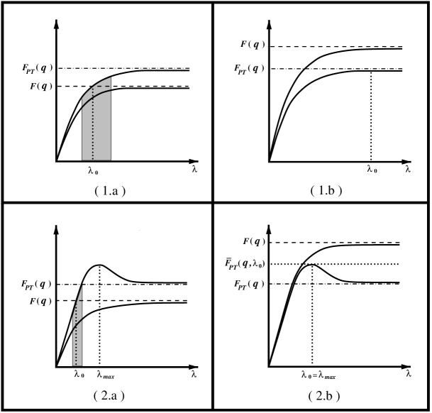
Figure 4: The variation of $\bar{F}_{PT}(q,\lambda)$ and the expected $\bar{F}(q,\lambda)$ versus $\lambda$ at a fixed value $q>\Lambda^{2}$. In (1.a) and (2.a) the upper and the lower curves describe $\bar{F}_{PT}(q,\lambda)$ and $\bar{F}(q,\lambda)$ respectively. In (1.b) and (2.b) the upper and the lower curves describe $\bar{F}(q,\lambda)$ and $\bar{F}_{PT}(q,\lambda)$ respectively.

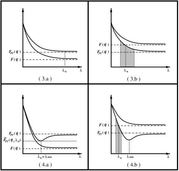
Figure 5: The variation of $\bar{F}_{PT}(q,\lambda)$ and the expected $\bar{F}(q,\lambda)$ versus $\lambda$ at a fixed value $q>\Lambda^{2}$. In (3.a) and (4.a) the upper and the lower curves describe $\bar{F}_{PT}(q,\lambda)$ and $\bar{F}(q,\lambda)$ respectively. In (3.b) and (4.b) the upper and the lower curves describe $\bar{F}(q,\lambda)$ and $\bar{F}_{PT}(q,\lambda)$ respectively.

For each of these four cases, there corresponds two possibilities either

(a) $$\hskip 7.22743ptF(q)<F_{PT}(q)\qquad\textrm{or}\,,$$

(b) $$\hskip 7.22743ptF(q)>F_{PT}(q)\,.$$

Accordingly, we shall denote the case associated with either possibility by case($i$.a) or case($i$.b) with $i=1,2,3\;\textrm{or}\;4$. These cases are illustrated in Fig.(4) and Fig.(5). In these figures, we include for each case an illustrative hypothetical graph for $\bar{F}(q,\lambda)$ based on our knowledge of the small and large behaviour of $\bar{F}(q,\lambda)$, i.e. $\bar{F}(q,\lambda)\cong\bar{F}_{PT}(q,\lambda)$ for sufficiently small $\lambda$ and $\bar{F}(q,\lambda)\cong F(q)$ for large enough $\lambda$. In applying our method we will need to know a priori whether $F_{PT}(q)$ is less than or greater than $F(q)$, either by input from an experiment or by a knowledge of the signs of higher order corrections to the perturbation theory in a regime where this can be trusted.

Our choice of $\lambda_{0}$ for the different cases, at a fixed value $q>\Lambda^{2}$, is as follows:

1. in case(1.a), the ideal value of $\lambda_{0}$ is the one at which $\bar{F}_{PT}(q,\lambda)$ intersects with $F(q)$ as shown in Fig.(4.1.a); such a point is not precisely known although it may be estimated from a knowledge of higher order corrections to $F_{PT}$ if these are available. We expect it to occur near the point of greatest curvature of $\bar{F}_{PT}(q,\lambda)$ as illustrated by the shaded region in Fig.(4.1.a). So for this case we might alternatively take $\lambda_{0}$ to be the value of $\lambda$ where the curvature is greatest.

2. in case(1.b), the monotonicity of $\bar{F}_{PT}(q,\lambda)$ means that sampling this curve at any finite value of $\lambda$ will fail to improve the perturbative estimate. However the use of a large, but finite value will depart little from the perturbative estimate (as the asymptotic behaviour is approached rapidly) and will have the merit of reinstating causality. So our best choice for $\lambda_{0}$ is the smallest $\lambda-$value at which $\bar{F}_{PT}(q,\lambda)$ is acceptably close to $F_{PT}(q)$.

3. in case(2.a), the ideal value of $\lambda_{0}$ is the one at which $\bar{F}_{PT}(q,\lambda)$ intersects with $F(q)$ as shown in Fig.(4.2.a); such a point is expected to lie within a narrow domain, on the left of $\lambda_{max}$, corresponding to a small arc segment just below $F_{PT}(q)$ as illustrated by the shaded region in Fig.(4.2.a); such a point might be estimated from a knowledge of higher order perturbative corrections; however without further information it is not possible to see how to identify this region from a knowledge of the perturbative function $\bar{F}_{PT}(q,\lambda)$ alone.

4. in case(2.b), the best choice for $\lambda_{0}$ is $\lambda_{max}$, as illustrated in Fig.(4.2.b), and this leads to an improvement over the perturbative estimate.

The cases depicted in Fig.(5) differ essentially by just a sign change, so a similar discussion of the appropriate choice of $\lambda_{0}$ can be made.

To summarise, from a prior knowledge of whether the perturbative estimate overshoots or undershoots the true value of the observable $F(q)$, and by plotting the shape of $\bar{F}_{PT}(q,\lambda)$ against $\lambda$ we can ascertain which of the various possible cases occurs in a given situation. For cases (1.a), (2.a), (3.b) and (4.b), there exists a unique point $\lambda=\lambda_{0}$ at which $\bar{F}_{PT}(q,\lambda_{0})$ matches the observable $F(q)$. However, for cases (2.b) and (4.a) the situation is different but still there is a point $\lambda_{0}$ at which $\bar{F}_{PT}(q,\lambda_{0})$ can give a bitter result than that of perturbation theory. In all of these cases, we can estimate $\lambda_{0}$ from the properties of $\bar{F}_{PT}(q,\lambda)$, or with the aid of higher order perturbative corrections, in a way that will improve on the perturbative predictions. On the other hand, in the remaining two cases (1.b) and (3.a) such an improvement does not occur.

Having determined $\lambda_{0}$ as a function of $q$ in a domain where perturbation theory is reasonably trustworthy, we use its average $\lambda_{e}$ in $\bar{F}_{PT}(q,\lambda_{e})$ to extrapolate to smaller values of $q$. This results in an estimate free of the unphysical divergences of the original perturbative approximation, and this is the central goal of our approach. This will be true even for the cases (1.b) and (3.a). In some cases, the effective average value $\lambda_{e}$ is either equal to or not significantly different from $\lambda_{0}(q)$. This is always true if $\lambda_{0}(q)$ is either a constant or a slowly varying function over a large domain of $q$. For instance, in our illustrative example $\lambda_{e}$ assumes the value $\lambda_{max}$ in case(2.b) and $\lambda_{min}$ in case(4.a); in other words it coincides with $\lambda_{0}(q)$ for all $q>\Lambda^{2}$. Also, it follows from the inequality:

$$|\Upsilon_{IR}(q,\lambda_{e})|\leq\,\frac{|U(\Lambda^{2})|}{q-\Lambda^{2}}\;\;{\mathrm{e}}^{-\lambda_{e}(q-\Lambda^{2})}+\frac{|\omega|}{\pi\Lambda^{2}}\>\frac{{\mathrm{e}}^{-\lambda_{e}q}}{\lambda_{e}\,q}\qquad\textrm{for}\;\>q\neq\Lambda^{2}\,,$$ (45)

that the contribution of $\Upsilon_{IR}(q,\lambda_{e})$ becomes negligible for $q\gg\Lambda^{2}$. Hence, employing $\lambda_{e}$ in the remote UV region does not spoil the standard perturbative results.

One final point to remark is that the method also applies in the reverse direction to the previous setting. For example, in the case when the infrared behaviour $F_{IR}(q)$ is well known then a similar representation to (7), but with $q$ replaced by a variable with the dimensions of length squared $r=1/q$, can be used in almost the same way as before except this time to deduce the corresponding analytic UV expression:

$$\bar{F}_{UV}(q=1/r,\lambda)=\frac{1}{2\pi i}\,\int_{C_{IR}}\,\,\frac{{\mathrm{e}}^{\lambda(\bar{r}-r)}}{\bar{r}-r}\,\,F_{IR}(1/\bar{r})\;d\bar{r}\,.$$ (46)

From this viewpoint, our method plays the role of a bridge between regions of small and large momenta, allowing us from a prior knowledge of either the UV or IR behaviour to extract information about the IR or UV properties respectively.

3 Analysis of the one-loop QCD running coupling

In this section, we demonstrate the implementation of our method in constructing a simple analytic model for describing the regular IR behaviour of the QCD effective coupling constant. For ease of calculation, we assume that the zeros of the exact function $\alpha(Q^{2})$ of the running coupling are expected to occur only on the negative real axis $\mathrm{Re}\{Q^{2}\}<0$ and/or infinity. This, together with the causality principle, allows us to express the reciprocal of $\alpha(Q^{2})$ in terms of the contour integral:

$$\frac{1}{\alpha(Q^{2})}=\frac{1}{2\pi i}\>\lim_{\lambda\rightarrow\infty}\>\;\int_{C_{UV}}\,\,\frac{{\mathrm{e}}^{\lambda(k-Q^{2})}}{k-Q^{2}}\>\>\frac{1}{\alpha(k)}\>\;dk\,,$$ (47)

introduced in the previous section. When applying this representation to an n-loop perturbative expression $\alpha^{(n)}_{\mathrm{PT}}(Q^{2})$, we take $\lambda=\lambda_{e}$ instead of $\infty$. In this way, we obtain a combination of perturbative and non-perturbative contributions, which has the merit of:

1. reinstating the causal analyticity structure in the right half plane $\mathrm{Re}\{Q^{2}\}\!\geq\!0$,

2. preserving the standard UV behaviour and,

3. improving the perturbative estimate in both the IR and low UV regions.

In the following, we shall prove this claim within the one-loop approximation. For convenience, we express the reciprocal of $\alpha^{(1)}_{\mathrm{PT}}(Q^{2})$ in terms of a dimensionless variable $q=Q^{2}/\Lambda^{2}$ as:

$$\frac{1}{\alpha^{(1)}(q)}=\frac{\beta_{0}}{4\pi}\,\ln(q)\,,$$ (48)

where $\alpha^{(1)}(Q^{2}/\Lambda^{2})=\alpha^{(1)}_{\mathrm{PT}}(Q^{2})$ . In the spirit of (47), an analytically improved expression corresponding to the one-loop coupling constant can be defined as:

$$\bar{\alpha}^{(1)}(q,\lambda_{e})=\frac{1}{\bar{\chi}^{(1)}(q,\lambda)}\,\Bigg{|}_{\lambda=\lambda_{e}}\,,$$ (49)

with

$$\bar{\chi}^{(1)}(q,\lambda)=\frac{1}{2\pi i}\,\int_{C_{UV}}\,\,\frac{{\mathrm{e}}^{\lambda(k-q)}}{k-q}\;\>\frac{1}{\alpha^{(1)}(k)}\;dk\,.$$ (50)

Note that $[\alpha^{(1)}(k)]^{-1}$, being dependent on $\ln q$, has a cut along the negative real axis $\textrm{Re}\{k\}\leq 0$. We shall now proceed to evaluate the above integral for the case $q\neq 0$. Following the same argument of the preceding section from (7) to (10), we can show that:

$$\bar{\chi}^{(1)}(q,\lambda)=\frac{\beta_{0}}{4\pi}\,\ln(q)+\frac{\beta_{0}}{4\pi}\,I_{C_{k}}(q,\lambda)\,,$$ (51)

where

$$I_{C_{k}}(q,\lambda)=\mathrm{J}_{\epsilon}(q,\lambda)+\int^{R_{\scriptscriptstyle{\mathrm{UV}}}}_{\epsilon}\;\frac{{\mathrm{e}}^{-\lambda(k+q)}}{k+q}\;dk\,,$$ (52)

with

$$\mathrm{J}_{\epsilon}(q,\lambda)=\frac{\epsilon\,{\mathrm{e}}^{-\lambda q}}{2\pi}\;\int^{\pi}_{-\pi}\,{\mathrm{e}}^{\lambda\epsilon\cos(\theta)}\;\;\textrm{Re}\left(\frac{{\mathrm{e}}^{i\lambda\epsilon\sin(\theta)}\,\ln(\epsilon\;{\mathrm{e}}^{i\theta})}{\epsilon-q\,{\mathrm{e}}^{-i\theta}}\right)\,d\theta\,.$$ (53)

A simple way to check that the contribution of $\mathrm{J}_{\epsilon}(q,\lambda)$ vanishes as $\epsilon$ approaches zero is to consider the upper bound:

$$|\mathrm{J}_{\epsilon}(q,\lambda)|\leq\;\frac{{\mathrm{e}}^{-\lambda(q-\epsilon)}}{q-\epsilon}\;\;\epsilon\,\left(\ln^{2}(\epsilon)+\pi^{2}\right)^{1/2}\,,$$ (54)

from which it follows that:

$$\lim_{\epsilon\rightarrow 0}\;\mathrm{J}_{\epsilon}(q,\lambda)=0\,.$$ (55)

Consequently, in the limit as $\epsilon\to 0$ we can write in a simple form:

$$I_{C_{k}}(q,\lambda)=\,\int^{R_{\mathrm{UV}}}_{0}\,\frac{{\mathrm{e}}^{-\lambda(k+q)}}{(k+q)}\,dk\;=E_{1}(\lambda q)-E_{1}(\lambda(q+R_{\mathrm{\scriptscriptstyle{UV}}}))\,.$$ (56)

By inserting this into (51) and letting $R_{\mathrm{\scriptscriptstyle{UV}}}\to\infty$, we obtain:

$$\bar{\chi}^{(1)}(q,\lambda)=\frac{\beta_{0}}{4\pi}\,\Big{[}\,\ln(q)+E_{1}(\lambda\,q)\,\Big{]}\,.$$ (57)

Having found the exact structure of $\bar{\chi}^{(1)}(q,\lambda)$ for $q\neq 0$, let us now reconsider the contour integral (50) once more to explore the continuity of $\bar{\chi}^{(1)}(q,\lambda)$ at the origin $q=0$. Starting from the expression:

$$\bar{\chi}^{(1)}(0,\lambda)=\frac{\beta_{0}}{4\pi}\frac{1}{2\pi i}\,\int_{C_{UV}}\,\,\frac{{\mathrm{e}}^{\lambda k}}{k}\,\ln(k)\,dk\,,$$ (58)

we arrive, after some work, at

$$\bar{\chi}^{(1)}(0,\lambda)= \frac{\beta_{0}}{4\pi}\,\lim_{\epsilon\rightarrow 0}\,\Bigg{[}\;\int_{\epsilon}^{R_{\mathrm{UV}}}\,\,\frac{{\mathrm{e}}^{-\lambda k}}{k}\,dk\,+\,\frac{\ln(\epsilon)}{\pi}\,\int_{0}^{\pi}\,{\mathrm{e}}^{\lambda\epsilon\cos(\theta)}\;\cos(\lambda\epsilon\sin(\theta))\;d\theta$$

$$\qquad\quad-\frac{1}{\pi}\,\int_{0}^{\pi}\,{\mathrm{e}}^{\lambda\epsilon\cos(\theta)}\;\sin(\lambda\epsilon\sin(\theta))\,\theta\;d\theta\>\,\Bigg{]}\,.$$ (59)

Making use of

$$\int_{\epsilon}^{R_{\mathrm{UV}}}\,\,\frac{{\mathrm{e}}^{-\lambda k}}{k}\,dk\,=E_{1}(\lambda\epsilon)-E_{1}(\lambda R_{\scriptscriptstyle{\mathrm{UV}}})\,,$$ (60)

and inserting the following series representations [16]:

$${\mathrm{e}}^{\lambda\epsilon\cos(\theta)}\;\cos(\lambda\epsilon\sin(\theta))= \sum_{n=0}^{\infty}\;\frac{(\lambda\epsilon)^{n}}{n!}\;\cos(n\theta)\qquad\textrm{for}\;\;\lambda\epsilon<1\,,$$

$${\mathrm{e}}^{\lambda\epsilon\cos(\theta)}\;\sin(\lambda\epsilon\sin(\theta))= \sum_{n=1}^{\infty}\;\frac{(\lambda\epsilon)^{n}}{n!}\;\sin(n\theta)\qquad\textrm{for}\;\;\lambda\epsilon<1\,,$$

into the two angular integrals in (59), we immediately obtain:

$$\bar{\chi}^{(1)}(0,\lambda)=\frac{\beta_{0}}{4\pi}\,\lim_{\epsilon\rightarrow 0}\,\Bigg{[}\;E_{1}(\lambda\epsilon)-E_{1}(\lambda R_{\mathrm{\scriptscriptstyle{UV}}})+\,\ln(\epsilon)+\sum_{n=1}^{\infty}\;\frac{(-1)^{n}}{n!\,n}\;(\lambda\epsilon)^{n}\>\,\Bigg{]}\,.$$ (61)

If we now make use of (27) and let $R_{\mathrm{\scriptscriptstyle{UV}}}\to\infty$, we arrive at:

$$\bar{\chi}^{(1)}(0,\lambda)=\frac{\beta_{0}}{4\pi}\,\ln({\mathrm{e}}^{-\gamma}/\lambda)\,.$$ (62)

This ensures the continuity condition at the origin:

$$\lim_{q\rightarrow 0}\;\bar{\chi}^{(1)}(q,\lambda)=\bar{\chi}^{(1)}(0,\lambda)\,.$$ (63)

Let us now find the range of $\lambda$ for which:

$$\bar{\alpha}^{(1)}(q,\lambda)=\frac{1}{\bar{\chi}^{(1)}(q,\lambda)}=\frac{4\pi}{\beta_{0}}\,\frac{1}{[\;\ln(q)+E_{1}(\lambda\,q)\;]}\,,$$ (64)

is continuous on the whole interval $q\geq 0$. This requires an investigation of the zeros of $\bar{\chi}^{(1)}(q,\lambda)$ in $D_{\bar{\chi}}$, where $D_{\bar{\chi}}=\{(q,\lambda):q\geq 0,\;\lambda>0\}$. From expression (57), we know that since $E_{1}(\lambda\,q)>0$ in $D_{\bar{\chi}}$ and $\ln q$ is negative only when $q\in(0,1)$, the zeros of the function $\bar{\chi}^{(1)}(q,\lambda)$ are expected to occur somewhere in the subinterval$\{(q,\lambda):0\leq q<1,\;\lambda>0\}\subset D_{\bar{\chi}}$. This domain can be reduced further by first considering the complementary exponential integral:

$$Ein(x)=\int_{0}^{1}\frac{[1-\mathrm{e}^{-xt}]}{t}\;dt=\sum_{n=1}^{\infty}\,\frac{(-1)^{n-1}}{n}\;\frac{x^{n}}{n!}\,,\qquad x\geq 0\,,$$ (65)

to rewrite (57) as:

$$\bar{\chi}^{(1)}(q,\lambda)=\frac{\beta_{0}}{4\pi}\,[\;\ln(\mathrm{e}^{-\gamma}/\lambda)+Ein(\lambda\,q)\;]\,.$$ (66)

Then by observing the fact that $Ein(\lambda\,q)\geq 0$ for all $\lambda\,q\geq 0$ and that $\ln(\mathrm{e}^{-\gamma}/\lambda)<0$ only if $\lambda>\mathrm{e}^{-\gamma}$, we deduce that the zeros of $\bar{\chi}^{(1)}(q,\lambda)$ can exist only in the following interval $\{(q,\lambda):0\leq q<1,\;\lambda\geq\mathrm{e}^{-\gamma}\}$. Hence, $\bar{\alpha}^{(1)}(q,\lambda)$ is continuous for all $q\geq 0$ if and only if $\lambda\in(0,\mathrm{e}^{-\gamma})$. Another way to obtain this result is by considering the fact that $\bar{\alpha}^{(1)}(0,\lambda)\geq\bar{\alpha}^{(1)}(q,\lambda)$ for all values of $\lambda$ that keep $\bar{\alpha}^{(1)}(q,\lambda)$ finite and positive throughout the range $q\geq 0$. Then, from the positivity of:

Figure 6: The zeros of $\bar{\chi}^{(1)}(q,\lambda)$: the curve shown in the strip $\{(q,\lambda):0\leq q<1,\;\lambda\geq e^{-\gamma}\}$ represents the roots of $\bar{\chi}^{(1)}(q,\lambda)$ in $D_{\bar{\chi}}$. This curve never touches the vertical $q=1$ as $\bar{\chi}^{(1)}(q,\lambda)$ does not have a zero on this line.

$$\bar{\alpha}^{(1)}(0,\lambda)=\frac{4\pi}{\beta_{0}}\;\frac{1}{\ln({\mathrm{e}}^{-\gamma}/\lambda)}\,,$$ (67)

it follows that the allowed values of $\lambda$ are those confined to the interval:

$$D_{eff}=\{\lambda\,:\;0<\lambda<{\mathrm{e}}^{-\gamma}\approx 0.561\}\,.$$ (68)

Using Maple VI for solving $\bar{\chi}^{(1)}(q,\lambda)=0$ numerically, we illustrate in Fig.(6) the zeros of $\bar{\chi}^{(1)}(q,\lambda)$, i.e the singularities of $\bar{\alpha}^{(1)}(q,\lambda)$, by a curve confined to the strip $\{(q,\lambda):0\leq q<1,\;\lambda\geq e^{-\gamma}\}$, showing that $D_{eff}$ is the only region of $\lambda$ for which $\bar{\alpha}^{(1)}(q,\lambda)$ is continuous for all $q\geq 0$.

4 The Estimation of $\lambda_{e}$

In this section, we try to find an effective value $\lambda_{e}\in D_{eff}$ such that $\bar{\alpha}^{(1)}(q,\lambda_{e})$ provides a better estimate than that of the standard perturbative results, especially in the vicinity of the Landau-pole and the IR region.

From the constraint (68), i.e. $\lambda_{e}\in D_{eff}$, it follows that:

$$0<\bar{\alpha}^{(1)}(q,\lambda_{e})<\textrm{M(q)}\qquad\textrm{for all}\;\;q\geq 0\,,$$ (69)

where the upper bound $\textrm{M(q)}=\bar{\alpha}^{(1)}(q,{\mathrm{e}}^{-\gamma})$. This implies that $\bar{\alpha}^{(1)}(q,\lambda_{e})<\alpha^{(1)}(q)=\bar{\alpha}^{(1)}(q,\lambda\gg 1)$ for all $q>1$. However, since $E_{1}(\lambda_{e}\,q)$ in (64) is negligibly small for $q\gg\lambda_{e}$, we may consider $\bar{\alpha}^{(1)}(q,\lambda_{e})=\alpha^{(1)}(q)$ at sufficiently large values of $q$. For a given $n_{f}$ and $q>1$, we find that the way in which $\bar{\alpha}^{(1)}(q,\lambda)$ changes with $\lambda$, as shown in Fig.(7), is a typical example of case(1) illustrated in Fig.(4).

Figure 7: The variation of $\bar{\alpha}^{(1)}(2,\lambda)$ versus $\lambda$, (a) for $n_{f}=3$ and (b) for $0\leq n_{f}\leq 6$. Here, $\bar{\alpha}^{(1)}(2,\lambda)$ tends to $\alpha^{(1)}(2)$ as $\lambda$ increases. In (b), $\bar{\alpha}^{(1)}(2,\lambda)$ increases with $n_{f}$ for any fixed value of $\lambda$.

Hence, before setting up a criterion for determining $\lambda_{e}$, we need to find out whether the perturbative estimate $\alpha^{(1)}(q)$, in the low UV region, overshoots or undershoots the true value $\alpha(q)$. This can be deduced by comparing $\alpha^{(1)}(q)$ to the standard higher-loop corrections [17]:

$$\alpha^{(2)}(q)=\frac{4\pi}{\beta_{0}\,L}\>\Big{[}1-\frac{\beta_{1}}{\beta_{0}^{2}}\>\frac{\ln L}{L}\Big{]}\,,$$ (70)

and

$$\alpha^{(3)}(q)=\frac{4\pi}{\beta_{0}\,L}\>\Big{[}1-\frac{\beta_{1}}{\beta_{0}^{2}}\>\frac{\ln L}{L}+\frac{\beta_{1}^{2}\,\ln^{2}L-\beta_{1}^{2}\,\ln L+\beta_{2}\,\beta_{0}-\beta_{1}^{2}}{\beta_{0}^{4}\;L^{2}}\Big{]}\,,$$ (71)

where $L=\ln q\,$ with $q=Q^{2}/\Lambda^{2}$, and:

$$\beta_{1} = 102-\frac{38}{3}\,n_{f}\,,$$ (72)

$$\beta_{2} = \frac{2857}{2}-\frac{5033}{18}\,n_{f}+\frac{325}{54}\,n_{f}^{2}\,.$$ (73)

Fig.(8) illustrates the comparison in terms of the physical scale $Q$ [GeV].

Figure 8: The comparison between the 1-, 2- and 3-loop running coupling for $n_{f}=3$.

In this figure, we consider $n_{f}=3$ and take $\Lambda=$ 0.593 GeV, 0.495 GeV and 0.383 GeV for $\alpha^{(1)}_{\mathrm{PT}}(Q^{2})$, $\alpha^{(2)}_{\mathrm{PT}}(Q^{2})$ and $\alpha^{(3)}_{\mathrm{PT}}(Q^{2})$ respectively. The $\Lambda$ values are determined in the $\overline{\textrm{MS}}$ scheme from the experimentally measured $\tau-$lepton decay rate [18] given by:

$$R_{\tau}=2.9087\>(0.998+\delta_{p}^{(n)})=3.492\,,$$ (74)

where

$$\delta_{p}^{(n)}=\sum_{k=1}^{n}a_{k}\>\Bigg{(}\frac{\alpha^{(n)}_{\mathrm{PT}}(M_{\tau}^{2})}{\pi}\Bigg{)}^{k}\,,$$ (75)

here $n\leq 3$ denotes the $n^{th}$ loop order approximation, $a_{1}=1$, $a_{2}=5.20232$, $a_{3}=26.3659$ and $M_{\tau}=1.777$ GeV. In Fig.(8), we used $n_{f}=3$ as the average number of active quarks, ignoring complications due to quark thresholds. This is reasonable in the low energy interval $Q<3$ GeV. For a more precise description of the evolution of $\alpha^{(n)}_{\mathrm{PT}}(Q^{2})$ in a larger momentum interval, one should take into account the effects of quark thresholds. However, this does not change the overall picture illustrated in Fig.(8). Having now observed that $\alpha^{(1)}_{\mathrm{PT}}(Q^{2})>\alpha^{(2)}_{\mathrm{PT}}(Q^{2})>\alpha^{(3)}_{\mathrm{PT}}(Q^{2})$, we would expect $\alpha^{(1)}(q)$ to overshoot the true value of the coupling constant, at least for intermediate and sufficiently small values of $q$. This indicates that our problem is of the type classified earlier as case(1.a) and depicted in Fig.(4.1.a). Hence, we may ascertain that for every point $q>1$ there exists a proper value $\lambda_{0}(q)$ such that $\bar{\alpha}^{(1)}(q,\lambda_{0}(q))=\alpha(q)$, just as explained in case(1.a). One way to estimate $\lambda_{0}(q)$ is to first consider the curvature function of $\bar{\alpha}^{(1)}(q,\lambda)$:

$$K^{(1)}(\lambda,q)=\;\frac{|\bar{\alpha}^{(1)}_{\lambda\,\lambda}(q,\lambda)|}{\Big{[}\;1+(\bar{\alpha}^{(1)}_{\lambda}(q,\lambda))^{2}\,\Big{]}^{3/2}}\,,$$ (76)

for a fixed $q>1$, where

$$\bar{\alpha}^{(1)}_{\lambda}(q,\lambda) =\frac{\partial}{\partial\lambda}\bar{\alpha}^{(1)}(q,\lambda)=\frac{\beta_{0}}{4\pi}\,\big{[}\,\bar{\alpha}^{(1)}(q,\lambda)\,\big{]}^{2}\;\frac{\mathrm{e}^{-\lambda q}}{\lambda}\,,$$ (77)

$$\bar{\alpha}^{(1)}_{\lambda\,\lambda}(q,\lambda) =\frac{\partial^{2}}{\partial\lambda^{2}}\bar{\alpha}^{(1)}(q,\lambda)=\bar{\alpha}^{(1)}_{\lambda}(q,\lambda)\,\Big{[}\,\frac{\beta_{0}}{2\pi}\;\bar{\alpha}^{(1)}(q,\lambda)\;\frac{\mathrm{e}^{-\lambda q}}{\lambda}-\frac{1}{\lambda}-q\,\Big{]}\,.$$ (78)

Then take $\lambda_{0}(q)$ to be the value of $\lambda$ at which $K^{(1)}(\lambda_{0},q)$ is a local maximum. For sufficiently small values of $q>1$, $K^{(1)}(\lambda,q)$ has two local maxima, say at $\lambda_{1}$ and $\lambda_{2}$. In this case, we consider $\lambda_{0}$ to be the largest of these (say $\lambda_{0}=\lambda_{2}>\lambda_{1}$) so that $\bar{\alpha}^{(1)}(q,\lambda_{0})$ remains as close as possible to the perturbative results $\alpha^{(1)}(q)$, which are still reasonable for such values of $q$. In Fig.(9) we plot the curvature function $K^{(1)}(\lambda,q)$ versus $\lambda$ for some fixed values of $q$, illustrating in part (a) of the figure the difference between $\bar{\alpha}^{(1)}(q,\lambda_{0})$ and $\alpha^{(1)}(q)$ for $q=3$. In part (b) of Fig.(9), we observe that the value of $\lambda_{0}$ decreases with increasing $q$.

Figure 9: The variation of $K^{(1)}(\lambda;q)$ versus $\lambda$ for $n_{f}=3$, (a) at $q=3$ and (b) at $q=3,4,5$. For a fixed $q>1$, $\,\lambda_{0}(q)$ denotes the value of $\lambda$ at which $K^{(1)}(\lambda;q)$ is a local maximum.In (b), $\lambda_{0}(5)<\lambda_{0}(4)<\lambda_{0}(3)$.

In general, if we plot $\lambda_{0}$ against $q$ for any quark flavour $n_{f}$ we find that $\lambda_{0}(q)$ is a monotonically decreasing function as shown in Fig.(10) for $n_{f}=3$.

Figure 10: The variation of $\lambda_{0}(q)$ versus $q$, for $n_{f}=3$.

Hence, we may express $D_{eff}$ in terms of $\lambda_{0}(q)$ as:

$$D_{eff}=\{\lambda_{e}:\lambda_{0}(\infty)<\lambda_{e}<\lambda_{0}(q_{0})\}\,,$$

with $q_{0}$ defined by $\lambda_{0}(q_{0})={\mathrm{e}}^{-\gamma}$. The values of $q_{0}$ for different $n_{f}$ are all given in table(1).

$n_{f}$ 0 1 2 3 4 5 6 $q_{0}$ 2.204 2.246 2.293 2.345 2.402 2.467 2.539

Table 1: Numerical values of $q_{0}(n_{f})$

For sufficiently large values of $q$, our choice of $\lambda_{0}$ does not lead to a significant improvement on the perturbative estimate. In fact, since only the first two decimal places of the coupling constant are of physical interest, we may take $\bar{\alpha}^{(1)}(q,\lambda_{0}(q))\cong\alpha^{(1)}(q)$ for all $q\geq 120$ and $0\leq n_{f}\leq 6$. On this basis, we shall focus our attention on the effective domain:

$$S_{eff}=\{\;q:\;q_{0}<q<120\;\}\,,$$ (79)

over which the difference between $\bar{\alpha}^{(1)}(q,\lambda_{0}(q))$ and $\alpha^{(1)}(q)$ is appreciable. Thus, we expect to find $\lambda_{e}$ in a narrower interval, $\bar{D}_{eff}=\{\lambda_{e}:\,\lambda_{0}(120)<\lambda_{e}<\lambda_{0}(q_{0})\}\subset\,D_{eff}\,$. Since, as illustrated in Fig.(10), $\lambda_{0}(q)$ is a very slowly varying function over a large part of the interval $S_{eff}$, i.e. for $q\in(11,120)$, we take the average of $\lambda_{0}(q)$ over $S_{eff}$ to be the best estimated value for $\lambda_{e}$. Our numerical results for $\lambda_{e}$ are listed in table(2) for the $n_{f}$ values of practical interest. As seen from table(2), the values of $\lambda_{e}$ do not change appreciably with $n_{f}$. Hence, we shall fix $\lambda_{e}$ to a central value of 0.04 for all $n_{f}$.

$n_{f}$ 0 1 2 3 4 5 6 $\lambda_{e}$ 0.0379 0.0390 0.0402 0.0416 0.0429 0.0444 0.0461

Table 2: Numerical values of $\lambda_{e}(n_{f})$

Let us now denote $\bar{\alpha}^{(1)}(Q^{2}/\Lambda^{2},\lambda_{e})$ by $\bar{\alpha}^{(1)}(Q^{2})$, where:

$$\bar{\alpha}^{(1)}(Q^{2})=\frac{4\pi}{\beta_{0}}\,\frac{1}{[\;\ln(Q^{2}/\Lambda^{2})+E_{1}(\lambda_{e}\,Q^{2}/\Lambda^{2})\;]}\,.$$ (80)

In this expression, the exponential integral function $E_{1}(\lambda_{e}\,Q^{2}/\Lambda^{2})$ plays an important role in removing the ghost pole at $Q=\Lambda$, preserving the correct UV behaviour (as it decays rapidly to zero for $Q\gg\Lambda$) and enforcing the running coupling to freeze in the low IR region. Therefore, it is essentially non-perturbative. At low energies, $\bar{\alpha}^{(1)}(Q^{2})$ approximates well to the simple formula:

$$\bar{\alpha}^{(1)}(Q^{2})=\frac{4\pi}{\beta_{0}\,\kappa_{e}}\,\;\frac{\varpi^{2}}{\varpi^{2}+Q^{2}}\qquad\textrm{for}\quad 0\leq Q^{2}\leq\Lambda^{2}\,,$$ (81)

where $\kappa_{e}=\ln({\mathrm{e}}^{-\gamma}/\lambda_{e})$ and $\varpi^{2}=\kappa_{e}\;\Lambda^{2}/\lambda_{e}$. In particular, this yields a finite value at the origin, namely:

$$\bar{\alpha}^{(1)}(0)=\frac{4\pi}{\beta_{0}\,\kappa_{e}}\,,$$ (82)

which is totally independent of the characteristic mass scale $\Lambda$. Obviously, this is a key advantage of our approach as it agrees with the IR freezing phenomenological hypothesis [11, 12]. Now, let me remark from Ref.[12] that the freezing phenomenon is not incompatible with confinement as there is no evidence that confinement necessarily requires the coupling constant to become infinite in the IR region. For instance, Gribov’s ideas [12, 13] explicitly involve a freezing of the coupling constant at low momenta. This phenomenon is also present in perturbation theory but beyond the leading order and for certain numbers of quark flavours.

5 Empirical Investigations of Our Model

In this section, we compare our approach with other recognised methods including conventional and modified perturbation theory. Then, we test our model on phenomenologically estimated data for a fit-invariant characteristic integral depending solely on the IR behaviour of the coupling constant.

5.1 Threshold Matching

In this subsection, we shall discuss the method we use for determining the values of $\Lambda^{(n_{f})}$ to be employed in our calculation. For sufficiently large values of $Q^{2}$, our expression for the coupling constant reduces to the familiar one-loop formula $\alpha^{(1)}_{\mathrm{PT}}(Q^{2})$. This suggests that our $\Lambda^{(n_{f})}$ must coincide with the usual QCD scale parameter $\Lambda^{(n_{f})}_{\mathrm{PT}}$ in momentum intervals corresponding to $n_{f}\geq 5$. Hence, we set our 5-flavour mass parameter $\Lambda^{(5)}$ equal to $\Lambda^{(5)}_{\mathrm{PT}}$ at the energy scale of the Z-boson mass $\mathrm{M}_{Z}=91.19$ GeV. We extract the value $\Lambda^{(5)}=0.135$ GeV from $\alpha^{(1)}_{\mathrm{PT}}(\mathrm{M}_{Z}^{2})$ by means of the recent parametrisation of the hadronic decay width of the Z-boson [19]:

$$R_{Z}=19.934\;\Bigg{[}1+\sum_{k=1}^{n}a_{k}\>\Bigg{(}\frac{\alpha^{(n)}_{\mathrm{PT}}(\mathrm{M}_{Z}^{2})}{\pi}\Bigg{)}^{k}\;\Bigg{]}\,,$$ (83)

where $n\leq 3$ denotes the $n^{th}$ loop order under consideration, $a_{1}=1.045$, $a_{2}=0.94$, $a_{3}=-15$ and $R_{Z}=20.768$ [20]. To obtain the values of $\Lambda^{(4)}$ and $\Lambda^{(3)}$, which may differ from $\Lambda^{(4)}_{\mathrm{PT}}$ and $\Lambda^{(3)}_{\mathrm{PT}}$ as they correspond to lower energy intervals, we use the familiar matching condition [23]:

$$\bar{\alpha}^{(1)}(Q_{th};n_{f})=\bar{\alpha}^{(1)}(Q_{th};n_{f}-1)\,,$$ (84)

at the energy thresholds $Q_{th}=2\,m_{b}$ and $Q_{th}=2\,m_{c}$, where $m_{b}=4.21$ GeV and $m_{c}=1.35$ GeV are the bottom- and charm-quark masses [11] respectively. In this way, starting with $\Lambda^{(5)}=0.135$ GeV, we get $\Lambda^{(4)}=0.188$ GeV and $\Lambda^{(3)}=0.229$ GeV.

At light quark thresholds $Q_{th}\leq 2\,m_{s}$, where $m_{s}=0.199$ GeV is the strange-quark mass [11], the applied matching condition (84) holds only approximately. This is also true for the analytic perturbation theory of Shirkov and Solovtsov [8]. For simplicity, instead of introducing a nontrivial and more complicated matching procedure such as the one used in Ref.[21], we choose to take $\Lambda^{(n_{f})}=\Lambda^{(3)}$ for all $n_{f}\leq 3$. This choice is quite reasonable since it leads to:

$$\frac{\bar{\alpha}^{(1)}(Q_{th};n_{f})}{\bar{\alpha}^{(1)}(Q_{th};n_{f}-1)}\cong 1\,,$$ (85)

for all energy thresholds corresponding to $n_{f}<3$. Furthermore, it is also supported by the good agreement with the value $\Lambda^{(0)}=0.238\,(0.019)$ GeV obtained from quenched lattice QCD in Ref. [22].

5.2 Illustrative comparison

We begin by considering a quick comparison between the predictions in our approach and those in perturbation theory at one-, two- and three-loop order.

 

Figure 11: The IR freezing behaviour of our model (a) and a comparison of our model with the 1-, 2- and 3-loop perturbative expressions (b).

Fig.(11) shows the behaviour of the 3-flavour running coupling $\bar{\alpha}^{(1)}(Q^{2})$ together with $\alpha^{(1)}_{\mathrm{PT}}(Q^{2})$, $\alpha^{(2)}_{\mathrm{PT}}(Q^{2})$ and $\alpha^{(3)}_{\mathrm{PT}}(Q^{2})$ in the low UV region as well as the Q-dependence of $\bar{\alpha}^{(1)}(Q^{2})$ outside the perturbative domain. In this plot we use the same $\Lambda$ values employed in Fig.(8) and take $\Lambda^{(3)}=0.229$ GeV for our formula $\bar{\alpha}^{(1)}(Q^{2})$. As is seen from Fig.(11.b), our model improves significantly on the 1-loop perturbative predictions and agrees well with the higher-loop estimates throughout the range $Q>1.5$ GeV. In Fig.(11.a), we observe that the evolution of $\bar{\alpha}^{(1)}(Q^{2})$ slows down appreciably as $Q$ enters the IR region, $Q\leq\Lambda^{(3)}$, and freezes rapidly to a finite value of 0.529. This provides some direct theoretical evidence for the freezing of the running coupling at low energies, an idea that has long been a popular and successful phenomenological hypothesis. Phenomenological studies, such as [11] and references therein, show that a running coupling that freezes at low energies can be useful in describing experimental data and some IR effects in QCD. In the low energy domain: $0.8\;\textrm{GeV}\leq Q\leq 1.2\;\textrm{GeV}\,,$ Badalian and Morgunov [24] extracted the value of the strong coupling constant $\alpha_{s}(Q^{2})$ from the fits to charmonium spectrum and fine structure splittings. They found that $\alpha_{s}(Q^{2})=0.38\pm 0.03(exp.)\pm 0.04(theory)$. This agrees reasonably well with our prediction, $\bar{\alpha}^{(1)}(Q^{2})=0.42\pm 0.03$ in the same energy interval.

Within the 3-loop approximation of the optimized perturbation theory, Mattingly and Stevenson [11] found that the 2-flavour QCD running coupling $\alpha_{s}$ freezes below 0.3 GeV to a constant value of about 0.26 $\pi$. Although this value is quantitatively uncertain (while qualitatively unequivocal), it is not far off from our 1-loop prediction of 0.16 $\pi$.

A good theoretical approach which supports the IR freezing behaviour of our model follows from the work of Simonov and Badalian [3, 4]. They studied the non-perturbative contribution to the QCD running coupling on the basis of a new background field formalism, exploiting non-perturbative background correlation functions as a dynamical input. In this framework, the one- and two-loop running coupling constants [4]:

$$\alpha^{(1)}_{B}(Q^{2}) = \frac{4\,\pi}{\beta_{0}}\;\frac{1}{\ln[(Q^{2}+M^{2}_{B})/\Lambda_{B}^{2}]}\,,$$ (86)

$$\alpha^{(2)}_{B}(Q^{2}) = \frac{4\,\pi}{\beta_{0}}\;\frac{1}{\ln[(Q^{2}+M^{2}_{B})/\Lambda_{B}^{2}]}\;\Bigg{[}1-\frac{\beta_{1}}{\beta_{0}^{2}}\frac{\ln[\ln[(Q^{2}+M^{2}_{B})/\Lambda_{B}^{2}]]}{\ln[(Q^{2}+M^{2}_{B})/\Lambda_{B}^{2}]}\Bigg{]}\,,$$ (87)

were found to depend on a new parameter $M_{B}$ (similar to $\lambda_{e}$ in our model) known as the background mass. From a fit to the charmonium fine structure [24], it was found that $M_{B}=1.1$ GeV. In table(3), we list the values of $\Lambda_{B}^{(n_{f})}$ for $n_{f}\leq 5$ in leading order (LO) and next-to-leading order (NLO). They are obtained as described in Ref.[4], using $\Lambda_{\mathrm{PT}}^{(5)}=0.135$ GeV in LO and $\Lambda_{\mathrm{PT}}^{(5)}=0.274$ GeV in NLO, which is basically the same method that we used to obtain the values of our $\Lambda^{(n_{f})}$.

$n_{f}$ 0 1 2 3 4 5 $\Lambda_{B}^{(n_{f})}$ GeV 0.307 0.283 0.258 0.230 0.188 0.135 LO $\Lambda_{B}^{(n_{f})}$ GeV 0.569 0.553 0.535 0.509 0.414 0.274 NLO

Table 3: The values of $\Lambda_{B}^{(n_{f})}$ in LO and NLO

In Fig.(12), we display the comparison between the 3-flavour

 

Figure 12: Illustrative comparison of our formula $\bar{\alpha}^{(1)}(Q)$ with the LO and NLO expressions for the background coupling constants $\alpha^{(1)}_{B}(Q)$ and $\alpha^{(2)}_{B}(Q)$ for $n_{f}=3$ .

coupling constant in our approach and those in the new background field formalism calculated to leading and next-to-leading order. As shown in the figure, our low energy estimates lie approximately in the middle between the predictions of $\alpha_{B}^{(1)}(Q^{2})$ and $\alpha_{B}^{(2)}(Q^{2})$, indicating the self-consistency of our results. At the origin $Q=0$, our results differ from that obtained by Shirkov and Solovtsov [8] by a small multiplicative factor $\kappa^{-1}_{e}=0.38$, i.e. $\bar{\alpha}^{(1)}(0)=0.38\;\alpha^{(1)}_{\mathrm{an}}(0)$, on the other hand we find that the estimates of the background coupling constants $\alpha^{(1)}_{B}(0)$ and $\alpha^{(2)}_{B}(0)$ are much closer to our predictions than to $\alpha^{(1)}_{\mathrm{an}}(0)$. Table(4) lists our results for $\bar{\alpha}^{(1)}(0)$ together with $\alpha^{(1)}_{\mathrm{an}}(0)$, $\alpha^{(1)}_{B}(0)$ and $\alpha^{(2)}_{B}(0)$ for $0\leq n_{f}\leq 5$.

$n_{f}$ 0 1 2 3 4 5 $\bar{\alpha}^{(1)}(0)$ 0.432 0.460 0.492 0.529 0.571 0.620 $\alpha^{(1)}_{\mathrm{an}}(0)$ 1.142 1.216 1.300 1.396 1.508 1.639 $\alpha^{(1)}_{B}(0)$ 0.448 0.448 0.448 0.446 0.427 0.391 $\alpha^{(2)}_{B}(0)$ 0.713 0.713 0.714 0.705 0.576 0.447

Table 4: The values of $\bar{\alpha}^{(1)}(0)$ compared to those of $\alpha^{(1)}_{\mathrm{an}}(0)$, $\alpha^{(1)}_{B}(0)$ and $\alpha^{(2)}_{B}(0)$

The numerical value of our coupling constant $\bar{\alpha}^{(1)}(Q^{2})$, as shown in table(4), is reasonably small which supports the notion of an expansion in powers of $\bar{\alpha}^{(1)}$ at low momentum transfers. Phenomenological verification of this fact would be of large practical value. Gribov theory of confinement [13] demonstrates how colour confinement can be achieved in a field theory of light fermions interacting with comparatively small effective coupling, a fact of potentially great impact for enlarging the domain of applicability of perturbative ideology to the physics of hadrons and their interactions [9].

In a number of cases of the QCD calculations it is necessary to estimate integrals of the form [25, 26]:

$$F(Q^{2})=\int^{Q}_{0}\;\alpha_{s}(k^{2})\,\mathrm{f}(k)\,dk\,,$$ (88)

where $\mathrm{f}(k)$ is a smooth function behaving like $k^{p}$ at $k\ll Q$. In this integral, the interval of integration includes the IR region where the perturbative expression for the running coupling $\alpha_{s}(k^{2})$ is inapplicable. Hence, by introducing an IR matching scale $\mu_{I}$ such that $\Lambda\ll\mu_{I}\ll Q$ the contribution to integral (88) from the region $k>\mu_{I}$ can be calculated perturbatively. On the other hand, the portion of the integral below $\mu_{I}$ is expressed in Ref.[25] in terms of a non-perturbative parameter $\bar{\alpha}_{p}(\mu_{I})$ as:

$$\int^{\mu_{I}}_{0}\;\alpha_{s}(k^{2})\,k^{p}\,dk\,=\frac{\mu_{I}^{p+1}}{p+1}\>\bar{\alpha}_{p}(\mu_{I})$$ (89)

For $\mu_{I}=2$ GeV and $p=0$, an excellent fit to experimental data yields: $A(2\,\mathrm{GeV})=\bar{\alpha}_{0}(2\,\mathrm{GeV})/\pi=0.18\pm 0.03$ [9] and $A(2\,\mathrm{GeV})=0.17\pm 0.01$ [25]. These results agree reasonably well with our estimate for $A(2\,\mathrm{GeV})$, which is obtained from (89) by direct substitution of our 3-flavour formula (80) for $\alpha_{s}(k^{2})$, giving:

$$A(2\,\mathrm{GeV})=\frac{2}{9}\int^{2}_{0}\;\frac{1}{\ln(k^{2}/\Lambda^{2})+E_{1}(\lambda_{e}\,k^{2}/\Lambda^{2})}\,dk\,\cong 0.14\,.$$ (90)

Here $\lambda_{e}=0.04$ and $\Lambda=0.229$ GeV.

5.3 Gluon condensate

In QCD instantons are the best studied non-perturbative effects, leading to the formation of the gluon condensate, an important physical quantity defined as [28]:

$$K=\langle 0|\frac{\alpha_{s}}{\pi}\;G^{a}_{\mu\nu}G^{a}_{\mu\nu}|0\rangle\,,$$ (91)

where $G^{a}_{\mu\nu}$ is the gluon field strength tensor and $\alpha_{s}$ is the quark-gluon coupling constant. This can be related to the total vacuum energy density $\epsilon_{t}$ of QCD by means of the famous trace anomaly relation [27]:

$$\theta_{\mu\mu}=-\frac{\beta_{0}\;\alpha_{s}}{8\,\pi}\;G^{a}_{\mu\nu}G^{a}_{\mu\nu}+\sum^{n_{f}}_{q}\;m_{q}\,\overline{\Psi}_{q}\Psi_{q}+O(\alpha_{s}^{2})\,,$$ (92)

where $m_{q}$ and $\Psi_{q}$ denote the quark masses and spinor quark fields respectively. Sandwiching $\theta_{\mu\mu}$ between the QCD vacuum states in the chiral limit $(\textrm{i.e}.\,\;m_{q}=0)$ and on account of the relation $\langle 0|\theta_{\mu\mu}|0\rangle=4\epsilon_{t}$ [28, 27], one obtains:

$$K=-\frac{32}{\beta_{0}}\;\epsilon_{t}\,.$$ (93)

In the dilute instanton-gas approximation with $n_{f}=0$, a direct relation between the gluon condensate $K$ and the instanton density [28, 29]:

$$\rho(r)=b\,\Bigg{[}\frac{2\pi}{\alpha^{(1)}_{\mathrm{PT}}(r^{-2})}\Bigg{]}^{6}\;\exp\Bigg{(}-\frac{2\pi}{\alpha^{(1)}_{\mathrm{PT}}(r^{-2})}\Bigg{)}\,,$$ (94)

with $r\thickapprox 1/Q$ as the instanton scale size variable and $b=0.0015$ [29], can be represented in the form [28]:

$$K=16\,\int^{\mathrm{R_{c}}}_{0}\frac{\rho(r)}{r^{5}}\;dr\,,$$ (95)

where $\mathrm{R_{c}}$ is a cut-off introduced by hand to avoid the uncontrollable IR divergences. Since our formula for the running coupling (80) agrees reasonably well with the estimate of $\alpha^{(1)}_{\mathrm{PT}}$ at short distances $r<\mathrm{R_{c}}$ and is analytic for all $r\geq 0$, it is very tempting to use it in place of $\alpha^{(1)}_{\mathrm{PT}}$ to evaluate the integral in (95) in the limit $\mathrm{R_{c}}\to\infty$. If we do this, we arrive at:

$$K=0.25\times 11^{6}\,b\,\Lambda^{4}\,\int^{\infty}_{0}\,x^{6}\,[\,\ln(x^{-2})+E_{1}(\lambda_{e}\,x^{-2})\,]^{6}\,\exp[-\frac{11}{2}E_{1}(\lambda_{e}\,x^{-2})]\,dx\,,$$ (96)

here $\Lambda$ corresponds to $n_{f}=0$. A direct numerical integration of (96) yields:

$$K=4.8624\;\Lambda^{4}\,.$$ (97)

Using the value $\Lambda=0.229$ GeV, which we computed in subsection (5.1) for small $n_{f}$, we estimate the gluon condensate from (97) as $K=0.013\;\mathrm{GeV^{4}}$. This is in good agreement with the value phenomenologically estimated from the QCD sum rules approach [28], namely $\langle 0|\frac{\alpha_{s}}{\pi}\;G^{a}_{\mu\nu}G^{a}_{\mu\nu}|0\rangle\cong 0.012\;\mathrm{GeV^{4}}$. In addition, our estimate for the gluon condensate is also consistent with that calculated phenomenologically in Ref. [30] and found to be $K=0.014^{\,+0.0044}_{\,-0.0018}\;\mathrm{GeV^{4}}$. Note that if we had considered the value $\Lambda^{(0)}=0.238$ GeV, obtained from quenched lattice QCD in Ref. [22], instead of our estimated value of $\Lambda$, we would have then found $K$ to be 0.015 $\mathrm{GeV^{4}}$, which is still close enough to the two phenomenological estimates mentioned above. Hence, it may well follow that the instanton density $\rho(r)$ is more likely to reveal more realistic and useful information when expressed in terms of our analytic running coupling $\bar{\alpha}^{(1)}$.

 

Figure 13: The behaviour of the instanton density as expressed in terms of the running couplings (a) $\alpha^{(1)}_{\mathrm{PT}}$, and (b) $\bar{\alpha}^{(1)}$.

In Fig.(13), we shed some light on the dependence of $\rho(r)$ on the running couplings $\alpha^{(1)}_{\mathrm{PT}}$ and $\bar{\alpha}^{(1)}$ which we shall denote by $\rho_{\mathrm{PT}}(r)$ and $\bar{\rho}(r)$ respectively. As seen in Fig.(13), at short distances, say $\,r<\,0.6\;\scriptstyle{\mathrm{GeV}^{-1}}$, $\rho_{\mathrm{PT}}(r)$ and $\bar{\rho}(r)$ agree reasonably well whereas when we increase $r$ to sufficiently larger values $\rho_{\mathrm{PT}}(r)$ rises very rapidly towards infinity while $\bar{\rho}(r)$ stabilizes to a fixed density. This reflects the practical usefulness of our approach to the strong coupling constant.

5.4 QCD $\beta-$function and IR properties

In quantum chromodynamics, the renormalisation group $\beta-$function:

$$\beta(\alpha(Q^{2}))=Q^{2}\,\frac{d\,\alpha(Q^{2})}{d\,Q^{2}}\,,$$ (98)

has the perturbative expansion [31]:

$$\beta(\alpha)=-\alpha\,\sum^{\infty}_{n=0}\,\beta_{n}\,\left(\frac{\alpha}{4\,\pi}\right)^{n+1}\,,$$ (99)

where $\beta_{0}$, $\beta_{1}$ and $\beta_{2}$ are given by (1), (72) and (73) respectively and [32]:

$$\beta_{3}=29243.0-6946.30\,n_{f}+405.089\,n_{f}^{2}\,+1.49931\,n_{f}^{3}\,,$$ (100)

here the higher-order coefficients $\beta_{n}$ for $n>3$ have not been calculated till now. Generally speaking, (98) is the crucial equation that decides whether or not there is a so-called stable fixed point at the origin (i.e. whether $\beta(\alpha)=0$ for $\alpha=0$) of either the infrared or ultraviolet type, with implications for the absence or presence of asymptotic freedom in the gauge theory under consideration. The distinction between an infrared and an ultraviolet stable fixed point depends on whether the derivative $\beta^{\prime}(\alpha)>0$ or $\beta^{\prime}(\alpha)<0$ at $\alpha=0$ respectively. In both kinds of gauge theories (Abelian and non-Abelian), there is a stable fixed point at the origin but it turns out that, while $\beta^{\prime}(\alpha)>0$ (stable IR fixed point) for an Abelian gauge theory, the reverse is true for a non-Abelian gauge theory , i.e. $\beta^{\prime}(\alpha)<0$ (stable UV fixed point). In general, it is extremely difficult to establish the existence of stable fixed points of a quantum field theory of $\beta(\alpha)$ for $\alpha\neq 0$. In perturbative QCD, the one-, two-, three- and four-loop $\beta-$function with quark flavours $n_{f}\leq 6$ fail to exhibit any non-trivial zero that can be interpreted as a stable IR fixed point. Because of this, the perturbative QCD coupling constant $\alpha_{\mathrm{PT}}(Q^{2})$ blows up as $Q^{2}\to 0$.

Our main task in this section is to demonstrate how the $\beta-$function in our approach can provide useful information about the IR region that a truncated perturbative series can not. As a cross check on our method, we shall calculate the stable IR fixed point for any number of quark flavour and show that it is consistent with our previous result (82). Starting from (80) with $\bar{\alpha}^{(1)}$ being renamed as $\alpha$, our QCD $\beta-$function in accordance with the definition (98) assumes the form:

$$\bar{\beta}(\alpha)=-\frac{\beta_{0}}{4\,\pi}\,\alpha^{2}\;[1-{\mathrm{e}}^{-W(\alpha)}]\,,$$ (101)

where

$$W(\alpha)={\mathrm{e}}^{\phi(\alpha)}\,,$$ (102)

and the function $\phi(\alpha)$ is defined by the transcendental relation:

$$\phi(\alpha)+E_{1}(\,{\mathrm{e}}^{\phi(\alpha)}\,)=\frac{4\,\pi}{\beta_{0}\,\alpha}+\ln(\lambda_{e})\,.$$ (103)

In the following domains of $\alpha$:

$$D_{1}=\{\,\alpha:\phi(\alpha)\geq 3\,\}=\{\,\alpha:0<\alpha\leq 2.021\,\beta_{0}^{-1}\,\}\,,$$ (104)

and

$$D_{2}=\{\,\alpha:\phi(\alpha)\leq-4\,\}=\{\,\alpha:\,4.724\,\beta_{0}^{-1}\leq\alpha<4.757\,\beta_{0}^{-1}\,\}\,,$$ (105)

a good approximate solution of (103) can be found as:

$$\phi(\alpha)\cong\begin{cases}\displaystyle{\frac{4\pi}{\beta_{0}\alpha}}+\ln(\lambda_{e})-E_{1}(\lambda_{e}\,\exp{\big{(}\displaystyle{\frac{4\pi}{\beta_{0}\alpha}}\big{)}})&\text{if $\alpha\in D_{1}$},\\ \\ \ln\left(\displaystyle{\frac{4\pi}{\beta_{0}\alpha}}-\kappa_{e}\right)&\text{if $\alpha\in D_{2}$}.\end{cases}$$ (106)

We note that as $\alpha$ approaches zero, $\phi(\alpha)$ grows without limit, allowing (101) to reproduce the conventional one-loop QCD $\beta-$function. It follows from (101) that for all $n_{f}$ satisfying $\beta_{0}(n_{f})>0$ there exists a stable IR fixed point $\alpha_{\mathrm{FP}}$ identified by $W(\alpha_{\mathrm{FP}})=0$. Using the expansion of (27) in (103), we obtain, in the limit $W(\alpha)\to 0$, the function:

$$W(\alpha)=\displaystyle{\frac{4\pi}{\beta_{0}\alpha}}-\kappa_{e}\,,$$ (107)

from which $\alpha_{\mathrm{FP}}$ is found to be:

$$\alpha_{\mathrm{FP}}=\displaystyle{\frac{4\pi}{\beta_{0}\,\kappa_{e}}}\,.$$ (108)

This is completely consistent, as it should be, with our previous result (82).

For $6<n_{f}\leq 16$, the higher-order terms of the QCD $\beta-$function are known to permit the occurrence of IR fixed points. For example, for all values of $n_{f}$ such that $\beta_{0}(n_{f})>0$ and $\beta_{1}(n_{f})<0$ the two-loop $\beta-$function $\beta^{(2)}_{\mathrm{PT}}(\alpha)$ possesses a non-trivial IR fixed point given by:

$$\alpha^{(2)}_{\mathrm{FP}}=-\displaystyle{\frac{4\pi\,\beta_{0}}{\beta_{1}}}>0\,.$$ (109)

This may sound fine. However, the IR fixed points arising from the truncation of the perturbative series (99) are likely to be spurious. For instance, at the candidate value for $\alpha_{\mathrm{FP}}$, the first and second order terms in $\beta^{(2)}_{\mathrm{PT}}(\alpha)$ are equal in magnitude ( i.e. $|\beta_{0}\,\alpha^{(2)^{2}}_{\mathrm{FP}}/4\pi|=|\beta_{1}\,\alpha^{(2)^{3}}_{\mathrm{FP}}/(4\pi)^{2}|$ ), indicating the inefficiency of the two-loop approximation around the calculated IR fixed point (109). In fact, there is no way to prove that the IR fixed points extracted from perturbation theory alone are indeed the positive zeros of the true $\beta-$function or anywhere near them. However, it is still worthwhile to test the perturbative expansion (99) to 4-loop order against our model for the $\beta-$function. In Fig.(14), we demonstrate the full behaviour of our $\beta-$function together with its perturbative counterpart for $n_{f}=6$ and 9. As seen in the figure, the $\beta-$function in our approach $\bar{\beta}(\alpha)$ agrees very well with the correct perturbative predictions at and near the UV fixed point $\alpha=0$. As $\alpha$ leaves the region $D$, where $D=\{\alpha:0\leq\alpha\leq 2.7/\beta_{0}(n_{f})\,\}$, $\bar{\beta}(\alpha)$ starts to diverge significantly from $\beta^{(1)}_{\mathrm{PT}}(\alpha)$ and changes direction, turning back to zero in the limit $\alpha\to\alpha_{\mathrm{FP}}$ as depicted in Fig.(14.a) for $n_{f}=6$. The occurrence of IR fixed points in $\beta^{(2)}_{\mathrm{PT}}(\alpha)$, $\beta^{(3)}_{\mathrm{PT}}(\alpha)$ and $\beta^{(4)}_{\mathrm{PT}}(\alpha)$ takes place only if $n_{f}\in[9,16],[7,16]$ and [8,16] respectively. In these $n_{f}-$intervals, we find that the two-, three- and four-loop $\beta-$functions behave qualitatively like $\bar{\beta}(\alpha)$. This is illustrated in Fig.(14.b) with $\beta^{(3)}_{\mathrm{PT}}(\alpha)$ and $\beta^{(4)}_{\mathrm{PT}}(\alpha)$ for $n_{f}=9$. It would have been interesting to see whether this qualitatively similar behaviour continues beyond the 4-loop order. Unfortunately, we know of no existing argument or calculation that definitively answers this question.

  

Figure 14: The behaviour of the $\beta-$function in our approach and in perturbation theory for $n_{f}=6$ (a) and $n_{f}=9$ (b). In (a), the curves of $\beta^{(2)}_{\mathrm{PT}}(\alpha)$, $\beta^{(3)}_{\mathrm{PT}}(\alpha)$ and $\beta^{(4)}_{\mathrm{PT}}(\alpha)$ coincide and none of them achieves a perturbative IR fixed point. In (b), the locations of the fixed points are different but very close to each other.

In table(5), we list the values of the IR fixed points in our approach and those allowed in perturbation theory within the two-, three- and four-loop approximations for $6<n_{f}<16$.

$n_{f}$	7	8	9	10	11	12	13	14	15
$\alpha_{\mathrm{FP}}$	0.751	0.839	0.951	1.098	1.297	1.586	2.039	2.854	4.757
$\alpha^{(2)}_{\mathrm{FP}}$	*	*	5.236	2.208	1.234	0.754	0.468	0.278	0.143
$\alpha^{(3)}_{\mathrm{FP}}$	2.457	1.464	1.028	0.764	0.579	0.435	0.317	0.215	0.123
$\alpha^{(4)}_{\mathrm{FP}}$	*	1.550	1.072	0.815	0.626	0.470	0.337	0.224	0.126
$\alpha^{(4)}_{\mathrm{UVFP}}$	*	14.364	12.090	5.617	3.294	2.295	1.781	1.480	1.286

Table 5: The values of $\alpha_{\mathrm{FP}}$ compared to those of $\alpha^{(2)}_{\mathrm{FP}}$, $\alpha^{(3)}_{\mathrm{FP}}$ and $\alpha^{(4)}_{\mathrm{FP}}$. The $*$ sign denotes the non-existence of a positive fixed point.

For $n_{f}\in[8,16]$, the four-loop $\beta-$function $\beta^{(4)}_{\mathrm{PT}}$ has two positive roots. The smaller of these is an IR fixed point whereas the larger one is an UV fixed point. Thus, we shall denote the latter by $\alpha^{(4)}_{\mathrm{UVFP}}$. From table(5), we find that with increasing $n_{f}$ our IR fixed point $\alpha_{\mathrm{FP}}$ increases gradually whereas the perturbative roots $\alpha^{(2)}_{\mathrm{FP}}$, $\alpha^{(3)}_{\mathrm{FP}}$, $\alpha^{(4)}_{\mathrm{FP}}$ and $\alpha^{(4)}_{\mathrm{UVFP}}$ decrease to smaller values. However, for most values of $n_{f}$ we observe that the further $\alpha_{\mathrm{FP}}$ is from one root of some order, say $\alpha^{(n)}_{\mathrm{FP}}$, the closer it is to another root of different order, say $\alpha^{(n\pm 1)}_{\mathrm{FP}}$. For example, for any $n_{f}\in[8,10]$ we find $\alpha_{\mathrm{FP}}$ to be closer in magnitude to $\alpha^{(3)}_{\mathrm{FP}}$ and $\alpha^{(4)}_{\mathrm{FP}}$ than to $\alpha^{(2)}_{\mathrm{FP}}$ and $\alpha^{(4)}_{\mathrm{UVFP}}$. On the other hand, for any $n_{f}\in[12,14]$ our estimate for $\alpha_{\mathrm{FP}}$ is much closer to $\alpha^{(4)}_{\mathrm{UVFP}}$ than to any other value of the perturbative IR fixed points. Also, for $n_{f}=11$ we have $\alpha_{\mathrm{FP}}\approx\alpha^{(2)}_{\mathrm{FP}}$. This analysis may not be conclusive however it provides us with some element of truth about our estimate for the possible magnitude of the true IR fixed point.

It is noteworthy that (108) enables us to express $\lambda_{e}$ in terms of $\alpha_{\mathrm{FP}}$ as:

$$\lambda_{e}=\exp\left(-\gamma-\displaystyle{\frac{4\pi}{\beta_{0}\,\alpha_{\mathrm{FP}}}}\right)\,.$$ (110)

This could have a direct beneficial effect on our approach if accurate phenomenological estimates for the IR fixed points were available. Indeed, if this were the case (110) would then allow us to determine the only free parameter $\lambda_{e}$ in the theory straightforwardly. However, in the absence of this phenomenological data, the method we used in obtaining the value $\lambda_{e}=0.04$ remains an adequate alternative as it results in a good approximation for the QCD $\beta-$function with any number of quark flavours.

6 Conclusions

In this paper, we have developed a new approach for investigating physical observables of the type $F(Q^{2})$ in regions that are inaccessible to perturbative methods of quantum field theory. In this approach, we have exploited the causality condition to reformulate $F(Q^{2})$ as a limit as $\lambda\to\infty$ of a contour integral depending on $\lambda$. In this way, we have shown that the perturbatively violated analyticity structure of physical observables can be reinstated in, at least, the right half of the complex $Q^{2}$-plane by taking $\lambda=\lambda_{e}$ instead of $\infty$, where $\lambda_{e}>0$ is the only free parameter of the theory. Explicit guidelines for finding an appropriate value for $\lambda_{e}$ has been given with illustrative examples. We have also shown how our construction can play the role of a bridge between regions of small and large momenta, emphasising the fact that from a prior knowledge of either the UV or IR behaviour we can extract information about the IR or UV properties respectively. In fact, as our formalism incorporates non-perturbative effects it extends the range of applicability of perturbation theory to cover the whole energy domain.

We have demonstrated the implementation of our method in tackling the ghost-pole problem in QCD, giving a simple and new analytic one-loop expression for the strong coupling constant. As our approach incorporates an extra free parameter $\lambda_{e}$ in addition to $\Lambda$, we have included a special method of determining $\lambda_{e}$ from the UV behaviour of the $\lambda$-dependent coupling constant $\bar{\alpha}^{(1)}(q,\lambda)$. This method involves the calculation of the maximum curvature of $\bar{\alpha}^{(1)}(q,\lambda)$ in the UV region $q>1$ as explained and carried out numerically in section (4). In this framework, we have found the effective parameter $\lambda_{e}$ to be 0.04 for $\bar{\alpha}^{(1)}(q,\lambda_{e})$. Although our prescription of obtaining $\lambda_{e}$ via the maximum curvature procedure can be replaced by just tuning $\lambda_{e}$ to allow the coupling fit with the experimental data available, we find our estimates for $\lambda_{e}$ appropriate enough for our model, leading to a good agreement with the result $\alpha_{s}(Q^{2})=0.38\pm 0.03(exp)\pm 0.04(theory)$ extracted from the fits to charmonium spectrum and fine structure splittings [24] at a low energy scale $Q=1.0\pm 0.2$ GeV. A supplementary discussion of how to determine the QCD scale parameter $\Lambda$ in our model has also been considered.

A distinctive feature of our approach is that the running coupling freezes to a finite value at the origin $Q^{2}=0$, being consistent with a popular phenomenological hypothesis [11, 12] namely the IR freezing phenomenon. This has also been supported by Gribov theory of confinement which demonstrates how colour confinement can be achieved in a field theory of light fermions interacting with comparatively small effective coupling, a fact of potentially great impact for enlarging the domain of validity of perturbative ideology to the physics of hadrons and their interactions.

For illustration, we have carried out a comprehensive comparison between the predictions in our approach and those estimated by other theoretical methods. Besides, we have tested our model on a fit-invariant IR characteristic integral extracted from jet physics data [9, 25] over the energy interval $Q\leq 2\,\mathrm{GeV}$. This test shows a reasonable agreement with our prediction. For further applications, we have used our model for the running coupling to compute the gluon condensate and have shown that our result agrees very well with the value phenomenologically estimated from QCD sum rules [28]. Finally, we have calculated the $\beta-$function corresponding to our QCD coupling constant and have shown that it behaves qualitatively like its perturbative counterpart, when calculated beyond the leading order and with a number of quark flavours allowing for the occurrence of IR fixed points.

In further studies, it would be interesting to apply our analytic approach to improve the standard expressions for the running masses in perturbative QCD.

Acknowledgements I would like to thank Prof. Paul Mansfield for useful discussions on this topic.

References

- [1] H.D.Politzer, Phys. Rev. Lett. 30 (1973) 1346; D. J. Gross and F. Wilczek, Phys. Rev. Lett. 30 (1973) 1343.
- [2] G. Paris, Phys. Lett. B 76 (1978) 65; Phys. Lett. B 69 (1977) 109.
- [3] Yu. A. Simonov, Phys. Atom. Nucl. 58 (1995) 107; Yu. A. Simonov, JETP Lett. 57 (1993) 525.
- [4] A. M. Badalian and Yu. A. Simonov, Phys. Atom. Nucl. 60 (1997) 630.
- [5] G. Grunberg, Phys. Lett. B 372 (1996) 121.
- [6] E. Gardi, G. Grunbergi and M. Karliner, hep-ph/9806462.
- [7] B. R. Webber, JHEP 9810 (1998) 012 (hep-th/9805484).
- [8] D. V. Shirkov and I. L. Solovtsov, Phys. Rev. Lett. 79 (1997) 1209 (hep-ph/9704333); I. L. Solovtsov and D. V. Shirkov, hep-ph/9909305.
- [9] Yu. L. Dokshitzer, V. A. Khoze and S. I. Troyan, Phys. Rev. D 53 (1996) 89 (hep-ph/9506425).
- [10] A. I. Alekseev and B. A. Arbuzov, hep-ph/9704228
- [11] A. C. Mattingly and P. M. Stevenson, Phys. Rev. D 49 (1994) 437; Phys. Rev. Lett. 69 (1992) 1320
- [12] P. M. Stevenson, Phys. Lett. B 331 (1994) 187.
- [13] F. Close et al., Phys. Lett. B 319 (1993) 291; V. N. Gribov, Lund preprint LU-TP 91-7 (March 1991).
- [14] H. W. Wyld, Mathematical Methods for Physics, Perseus Books 1999.
- [15] G. Arfken, Mathematical Methods for Physicists, Academic Press 1985; A. Erdélyi et al., Higher Transcendental Functions, Vol. 2, McGraw-Hill Book Company, 1953.
- [16] I. S. Gradshteyn and I. M. Ryzhik, Table of Integrals, Series, and Products, Academic Press, 1980.
- [17] F. I. Ynduráin, The Theory of Quark and Gluon Interactions, Springer 1999.
- [18] J. G. Körner, F. Krajewski, A. A. Pivovarov, Phys. Rev. D 63 (2001) 036001; hep-ph/0002166
- [19] E. Tournefier, Proc. of the Quarks ’98 Int. Seminar, Suzdal, Russia, May 1998; hep-ex/9810042
- [20] The LEP Collaborations ALEPH, DELPHI, L3, OPAL, the LEP Electroweak Working Group and the SLD Heavy Flavour and Electroweak Groups, CERN-EP/2000-016.
- [21] K. G. Chetyrkin, J. H. Kühn and M. Steinhauser, hep-ph/0004189
- [22] S. Capitani, M. Lüscher, R. Sommer and H. Wittig, Nucl. Phys. B544 (1999) 669.
- [23] W. J. Marciano, Phys. Rev. D 29 (1984) 580.
- [24] A. M. Badalian and V. L. Morgunov, Phys. Rev. D 60 (1999) 116008 (hep-ph/9901430); A. M. Badalian and B. L. G. Bakker, Phys. Rev. D 62 (2000) 094031 (hep-ph/0004021).
- [25] Yu. L. Dokshitzer and B. R. Webber, Phys. Lett. B 352 (1995) 451.
- [26] Yu. L. Dokshitzer, hep-ph/9812252; A. I. Alekseev, hep-ph/9802372.
- [27] V. Gogohia and H. Toki, Phys. Lett. B 466 (1999) 305.
- [28] M. A. Shifman, A. I. Vainshtein and V. I. Zakharov, Nucl. Phys. B 147 (1979) 385, 448.
- [29] C. Bernard, Phys. Rev. D 19 (1979) 3013.
- [30] B. Guberina, R. Meckbach, R. D. Peccei and R. Rückl, Nucl. Phys. B184 (1981) 476.
- [31] R. K. Ellis, W. J. Stirling and B. R. Webber, QCD and Collider Physics, Cambridge University Press 1996.
- [32] T. van Ritbergen, J. A. M. Vermaseren and S. A. Larin, Phys. Lett. B 400 (1997) 379; S. A. Larin and J. A. M. Vermaseren, Phys. Lett. B 303 (1993) 334.