(Non-)Abelian Kramers–Wannier Duality
And Topological Field Theory

Abstract:

We study a connection between duality and topological field theories. First, 2d Kramers–Wannier duality is formulated as a simple 3d topological claim (more or less Poincaré duality), and a similar formulation is given for higher-dimensional cases. In this form they lead to simple TFTs with boundary coloured in two colours. The statistical models live on the boundary of these TFTs, as in the CS/WZW or AdS/CFT correspondence.

Classical models (Poisson–Lie T-duality) suggest a non-abelian generalization in the 2d case, with abelian groups replaced by quantum groups. Amazingly, the TFT formulation solves the problem without computation: quantum groups appear in pictures, independently of the classical motivation. Connection with Chern–Simons theory appears at the symplectic level, and also in the pictures of the Drinfeld double: Reshetikhin–Turaev invariants of links in 3-manifolds, computed from the double, are included in these TFTs. All this suggests nice phenomena in higher dimensions.

1 Introduction: KW duality as a 3-dimensional topological claim

Kramers–Wannier duality in 2d statistical models is a rather elementary equivalence between two models defined on mutually dual planar graphs. Yet it may be a bit surprising that one can give a two-line proof of its most general form (including all topological subtleties, order-disorder operator duality, etc.), together with its higher-dimensional generalizations. The basic idea is, roughly speaking, to consider surfaces that are boundaries of 3d bodies (or $n$-manifolds, boundaries of $n+1$-manifolds). As we shall see, the 2d models “live on the boundary” of a 3d topological field theory—an idea familiar from WZW/Chern–Simons correspondence, or from AdS/CFT duality. In this paper we try to study non-Abelian generalizations of KW-duality, following this connection with TFT.

The duality is a claim about pictures like this:

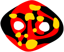
Figure 1: A mask

The picture represents a 3d body (a ritual mask) made of yellow material, with the surface partially painted in red and black. For definiteness imagine that the invisible side is unpainted (i.e. completely yellow). In general we have a compact oriented yellow $n+1$-fold $\Omega$ with the boundary coloured in this way (in a locally nice way; more precisely, $\Omega$ is a cobordism connecting yellow surfaces with boundaries colored in red and black).

We decompose $n$ as $n=k+l$ ($2=1+1$ in 2d statistical models) and choose a finite abelian group $G$ and its dual $\tilde{G}$. Let $y$ be the yellow part of the boundary; it is a compact oriented $n$-dim surface with the boundary coloured in black and red. The relative cohomology groups $H^{k}(y,r_{y};G)$ and $H^{l}(y,b_{y};\tilde{G})$ (both are finite Abelian groups) are mutually dual via Poincaré duality ($r_{X}$ denotes the red part of $X$; notice that $r_{y}=r_{\Omega}\cap y$). Let $\rho:H^{k}(\Omega,r_{\Omega};G)\rightarrow H^{k}(y,r_{y};G)$ and $\tilde{\rho}:H^{l}(\Omega,b_{\Omega};\tilde{G})\rightarrow H^{l}(y,b_{y};\tilde{G})$ be the restriction maps.

Theorem 1

(Kramers-Wannier duality)
The images of $\rho$ and $\tilde{\rho}$ are each other’s annihilators.

Proof. It is an immediate consequence of a piece of the long exact sequence of the triple $r_{\Omega}\subset y\cup r_{\Omega}\subset\Omega$,

$$H^{k}(\Omega,r_{\Omega};G)\rightarrow H^{k}(y\cup r_{\Omega},r_{\Omega};G)\rightarrow H^{k+1}(\Omega,y\cup r_{\Omega};G),$$

where the first arrow is (by excision) $\rho$ and the second (by Poincaré duality) is the adjoint of $\tilde{\rho}$, q.e.d.

In statistical models it is used in the following form: for any function $f:H^{k}(y,r_{y};G)\rightarrow\mathbb{C}$ (the Boltzmann weight) we define the partition sum

$$Z(f)=\sum_{x\in H^{k}(\Omega,r_{\Omega};G)}f(\rho(x)).$$ (1)

Let $\hat{f}$ denote the Fourier transform of $f$. We can define

$$\tilde{Z}(\hat{f})=\sum_{x\in H^{l}(\Omega,b_{\Omega};\tilde{G})}\hat{f}(\tilde{\rho}(x)).$$ (2)

Theorem 1 and Poisson summation formula now give

Corollary 1

(KW duality, usual form)
For some constant $c$ (independent of $f$), $Z(f)=c\tilde{Z}(\hat{f})$.

Let us stop to make a connection with more usual formulations. Notice that an element of $H^{1}(X,Y;G)$ is the same as (the isomorphism class of) a principal $G$-bundle over $X$ with a given section over $Y\subset X$. If $\Omega$ is a 3d ball (with coloured surface), an element of $H^{1}(\Omega,r_{\Omega};G)$ is therefore specified by choosing an element of $G$ for each red stain. We may imagine that there is a $G$-valued spin sitting at each such stain and, to compute (1.1), we take the sum over all their values (we overcount $|G|$ times, but it is inessential). According to KW duality, the same result can be obtained by summing over $\tilde{G}$-spins at the black stains. The spins at red (or black) stains interact through the yellow stains. If all the yellow stains are as those visible on the picture (disks with two red and two black neighbours), we have the usual two-point interactions; for disks with more neighbours we would have more-point interactions.

Finally, let us look at the picture again. It does not represent a ball and the back yellow stain is not a disk. The Boltzmann weight for the back stain can be understood as the specification of the boundary and periodicity conditions on the visible surface (the $G$-bundle type together with sections over the red parts of the boundary). The boundary and periodicity conditions at the holes can be interpreted as order and disorded operators respectively.

These examples are more or less all that we would like; the general case seems to be general beyond usual applications. But it will come handy when we consider non-abelian generalizations.

What are we going to do? First of all, expression (1.1) has the form of a very simple topological field theory (with boundary coloured in red and black), described in the next section. We shall then look at the non-abelian version. In the $2=1+1$ case classical models suggest that the pair $G$, $\tilde{G}$ should be replaced by a pair of mutually dual quantum groups. So we are faced with the difficult and somewhat arbitrary task of defining and understanding quantum analogues of cohomology groups and of the Poisson summation formula. But miraculously, none of these has to be done. Pictures alone (in the form of TFTs) solve the problem and quantum groups appear. This suggests, of course, that this point of view might be interesting in higher dimensions, the $4=2+2$ case—the electric–magnetic duality—being of particular interest.

2 KW TFTs and the squeezing property

As we mentioned, expression (1.1) has the form of a TFT with boundary coloured in red and black. We understand TFT as defined by Atiyah [1] and for definiteness we choose its hermitian version; nothing like central extensions is taken into account. To each oriented yellow $n$-dim $\Sigma$ with black-and-red boundary, we associate a non-zero finite-dimensional Hilbert space ${\cal H}(\Sigma)=L^{2}(H^{k}(\Sigma,r_{\Sigma};G))$. And for each $\Omega$ we have a linear form on the Hilbert space corresponding to $y$ – the one given by (1.1). However, the normalization has to be changed slightly for the gluing property to hold (this is only a technical problem): we set

$$Z_{\Omega}(f)={1\over\mu(\Omega)}\sum_{x\in H^{k}(\Omega,r_{\Omega};G)}f(\rho(x))$$ (3)

and for the inner product

$$\langle f,g\rangle=\mu(\Sigma)\sum_{x\in H^{k}(\Sigma,r_{\Sigma};G)}\overline{f(x)}g(x).$$ (4)

Here

$$\mu(\Omega)={|H^{k-1}(\Omega,r_{\Omega};G)||H^{k-3}(\Omega,r_{\Omega};G)|\dots\over|H^{k-2}(\Omega,r_{\Omega};G)||H^{k-4}(\Omega,r_{\Omega};G)|\dots}$$ (5)

(and the the same for $\Sigma$). Perhaps this $\mu$ is not a number you would like to meet in a dark forest, but this should not hide the simplicity of the thing. The gluing property follows from the exact sequence for the triple $r_{glued}\subset\Omega\cup r_{glued}\subset\Omega_{glued}$ ($r_{glued}$ is the red part of $\Omega_{glued}$; $\Omega\subset\Omega_{glued}$ is achieved by separating slightly the glued yellow surfaces). Of course, the expression for $\mu$ was actually derived from this sequence. Hence we can state

Theorem 2

The asignment $\Sigma\mapsto{\cal H}(\Sigma)$ and $\Omega\mapsto Z_{\Omega}$ is a TFT (for cobordisms with boundary colored in two colors).

This TFT reformulation of KW duality will be our starting point for non-abelian generalizations (the duality is an isomorphism between the TFT given by $G$ and $k$, and the TFT given by $\tilde{G}$ and $l$, with exchanged red and black). Let us first have a look to see if we can recover the numbers $k$ and $l$ and the group $G$ from the TFT. It is enough to take yellow $n$-dim balls as $\Sigma$’s. The ball should be painted as follows: let us choose integers $k^{\prime},l^{\prime}$ such that $k^{\prime}+l^{\prime}=n$; we take a $S^{k^{\prime}-1}\subset\partial\Sigma$ and paint its tubular neighbourhood in $\partial\Sigma$ in red; the rest (a tubular neighbourhood of a $S^{l^{\prime}-1}$) is in black. Let us denote this $\Sigma$ as $B^{n}_{k^{\prime},l^{\prime}}$. The corresponding Hilbert space ${\cal H}(B^{n}_{k^{\prime},l^{\prime}})$ is trivial (equal to $\mathbb{C}$) if $k^{\prime}\neq k$; if $k^{\prime}=k$, it is the space of functions on $G$. The reader may try to define the Hopf algebra structure on this space using pictures (the $2=1+1$-case is drawn in the next section).

Our TFTs are of a rather special nature, because of the excision property of relative cohomology. It gives rise to the squeezing property of our TFTs. It is best explained by using an example. Imagine this full cylinder (the upper half of its mantle is red and the lower half is black; the invisible base is yellow):

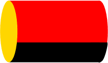
Figure 2: before…

We shall squeeze it in the middle, putting one finger on the red top and the other on the black bottom. The result is no longer a manifold—it has a rectangle in the middle (red from the top and black from the bottom), but it is surely homotopically equivalent (as a pair $(\Omega,r_{\Omega})$, or as a pair $(\Omega,b_{\Omega})$) to the original cylinder. Since we use relative cohomologies, the rectangle may be removed (it does not matter whether the cohomologies are relative to $r$ or to $b$ (the dual picture), as the rectangle is both red and black). The result is again a manifold of the type we admit:

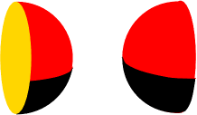
Figure 3: …and after

Or, as another example: if our fingers are not big enough, we do not separate the cylinder into two parts, but instead we produce a hole in the middle (the top view of the result would be a red stain with a hole in the middle).

A bit informally the squeezing property can be formulated as follows: if a (hyper)surface appears as a result of squeezing $\Omega$, red from one side and black from the other side, it may be removed. Using excision, we can state

Theorem 3

The TFTs of Theorem 2 satisfy the squeezing property.

Those TFTs that satisfy the squeezing property may be considered as generalizations of relative cohomology and of KW duality. As we shall see in the next setion, in the $2=1+1$-case they yield the expected result.

Example: Here is an example of such a TFT that does not come from an abelian group. We take a finite group $G$ and two subgroups $R,B\subset G$ such that $RB=G$, $R\cap B=1$. We shall consider principal $G$-bundles with reduction to $R$ over $r$ and to $B$ over $b$. If $P$ is such a thing, let $\mu(P)$ be the number of automorphisms of $P$. If $M$ is a space with some red and some black parts, let $P(M)$ be the set of isomorphism classes of these things. We set ${\cal H}(\Sigma)$ (the Hilbert space) to be the space of functions on $P(\Sigma)$ with the inner product

$$\langle f,g\rangle=\sum_{P\in P(\Sigma)}\mu(P)\overline{f(P)}g(P)$$ (6)

and finally, if $f\in{\cal H}(y)$, we set

$$Z_{\Omega}(f)=\sum_{P\in P(\Omega)}{1\over\mu(P)}f(P|_{y}).$$ (7)

This is surely a TFT. The squeezing property holds, because if we have a reduction for both $R$ and $B$ (as we have on the surfaces that appear by squeezing), these two reductions intersect in a section of the $G$-bundle. If $R=1$ and $B=G$, this TFT describes interacting $G$-spins (as in the introduction); the general case is more interesting, providing a non-trivial example for §3. We will also meet its version in §4.

3 Non-abelian $2=1+1$-duality

There are classical models (those appearing in Poisson–Lie T-duality [3]) that suggest a non-abelian generalization of $2=1+1$ KW duality. The PL T-duality generalizes the usual $R\leftrightarrow 1/R$ T-duality, replacing the two circles (or tori) by a pair of mutually dual PL groups. Clearly, we have to replace the pair $G$, $\tilde{G}$ by a pair of mutually dual quantum groups. This is not an easy (or well-defined) task. We have to define and to understand cohomologies with quantum coefficients.

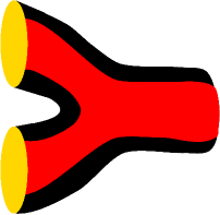
Figure 4: Product

Here is how pictures solve this problem in a very simple way: just take a TFT in three dimensions, satisfying the squeezing property. A finite quantum group (finite-dimensional Hopf $C^{*}$-algebra) will appear independently of the classical motivation. If you exchange red and black (which gives a new TFT), the quantum group will be replaced by its dual. This is the non-abelian (or quantum) $2=1+1$ KW duality.

Now we will draw the pictures. I learned this 3d way of representing quantum groups at a lecture by Kontsevich [4]; it was one of the sources of this work. The finite quantum group itself is ${\cal H}(B^{2}_{1,1})$. The product ${\cal H}(B^{2}_{1,1})\otimes{\cal H}(B^{2}_{1,1})\rightarrow{\cal H}(B^{2}_{1,1})$ is on fig. 4.

Figure 5: All operations

And here are all the operations. Coloured 3d objects are hard to draw (but not hard to visualize!); imagine that the pictures represent balls and that their invisible sides are completely yellow. The antipode $S$ is simply the half-turn, the involution $*$ is the reflection with respect to the horizontal diameter, and the rest is on the figure:

Why is it a quantum group? Just imagine the pictures representing the finite quantum group axioms and use the squeezing property in a very simple manner. We (more precisely, you) have proved

Theorem 4

A 3d TFT satisfying the squeezing property yields a finite quantum group.

Conjecture 1

There is a 1–1 correspondence between finite quantum groups and 3d TFTs satisfying the squeezing property, with trivial (i.e. one-dimensional) ${\cal H}(B^{2}_{0,2})$ and ${\cal H}(B^{2}_{2,0})$.

To support the conjecture, finite quantum groups are in 1–1 correspondence with modular functors of a certain kind (cf. [7]), clearly connected with our TFTs.

4 Chern–Simons with coloured boundary

Let us recall a basic analogy between symplectic manifolds and vector spaces (the aim of quantization is to go beyond a mere analogy):

Vector	Symplectic
Vector space	Symplectic manifold
Vector	Lagrangian submanifold
$V_{1}\otimes V_{2}$	$M_{1}\times M_{2}$
$V^{*}$	$\overline{M}$
Composition of linear maps	Composition of Lagrangian relations

One can easily describe the symplectic analogue of the Chern–Simons TFT (see e.g. [2]). Let ${\mathfrak{g}}$ be a Lie algebra with invariant inner product. If $\Sigma$ is a closed oriented surface then the moduli space of flat ${\mathfrak{g}}$-connections is a symplectic manifold (with singularities). The symplectic form is given as follows. The vector space of all ${\mathfrak{g}}$-valued 1-forms on $\Sigma$ is symplectic, with the symplectic form

$$\omega(\alpha_{1},\alpha_{2})=\int_{\Sigma}\langle\alpha_{1},\alpha_{2}\rangle.$$ (8)

When we restrict ourselves to flat connections, the space is no longer symplectic, but the null directions of the 2-form give just the orbits of the gauge group, so the quotient (the moduli space) is symplectic. Let us denote it by $M_{\Sigma}$.

We have associated a symplectic space to every oriented closed surface. Now, if $\Omega$ is an oriented compact 3-fold with boundary $\Sigma$, we should find a Lagrangian subspace $\Lambda_{\Omega}\subset M_{\Sigma}$. Indeed, $\Lambda_{\Omega}$ consists just of those flat connections on $\Sigma$, which can be extended to $\Omega$.

Let us make a minute extension of this construction, allowing a boundary coloured in red and black. Let ${\mathfrak{b}},{\mathfrak{r}}\subset{\mathfrak{g}}$ be a Manin triple. We shall consider flat ${\mathfrak{g}}$ connections as before, with the obvious boundary conditions—on the red part of the boundary the connection should take values in ${\mathfrak{r}}$ and on the black part in ${\mathfrak{b}}$. Similarly, the gauge group consists of the maps to $G$ with the same boundary conditions. This really defines a symplectic TFT for our pictures. From this symplectic TFT we obtain a symplectic analogue of quantum group (using the pictures of the previous section). One readily checks that it is the double symplectic groupoid of Lu and Weinstein [5]—the symplectic analogue of the quantum group coming from the Manin triple ${\mathfrak{b}},{\mathfrak{r}}\subset{\mathfrak{g}}$.

For this reason, it is reasonable to conjecture that perturbative quantization of our Chern–Simons TFT with boundary will give the corresponding quantum group.

In the next section we return to the vector side of our table, to general 3d TFTs that satisfy the squeezing property. We shall see this connection with CS TFTs again, in a different guise.

5 Pictures of the Drinfeld double

Figure 6: Double unit & counit,

There are lots of algebras, modules, etc., in our pictures. We shall describe only the Drinfeld double, since it is important in PL T-duality, and also to make a connection with Reshetikhin–Turaev invariants. Here are the unit and the counit:

The invisible side of the full torus on the first picture is yellow; this closed yellow strip is the double.

Figure 7: product,

On the second picture it is represented as the mantle of the cylinder (the invisible base of the cylinder is painted as the visible one).

The product (the picture is yellow from the invisible side) and coproduct are on figures 7 and 8. The last picture requires an explanation. It represents a thick Y from which a thin Y was removed (you can see it as the black holes in the yellow disks). The fronts of these Y’s are red and their backs are black (the invisible bottom of the picture is yellow—it is the third double).

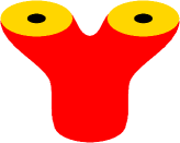
Figure 8:
coproduct,

For completeness, the antipode is a half-turn and the involution a reflection, both exchanging the boundary circles of the double.

Now we know the double as a Hopf algebra, but its real treasure is the $R$-matrix. It is quite similar to the Y-picture, but this time we do not remove a thin X, but rather two tubes connecting the top holes with the bottom ones. However, if one tube connected the left holes and the other one the right holes, the picture would not be very interesting. We could squeeze the X in the middle, dividing it into two vertical cylinders. We would simply have an identity.

Figure 9: and
$R$-matrix.

However, in the X of the $R$-matrix, the tubes are diagonal. There are two ways for them to avoid each other; one gives the $R$-matrix and the other its inverse. This X has two incoming and two outgoing doubles; you can also imagine $n$ doubles at the bottom, tubes forming a braid inside and leaving the body at the top, in the middle of $n$ other doubles (the Cyrillic letter ZH is good here). We directly see a representation of the braid group.

With this picture in mind, we can find the Reshetikhin–Turaev (RT) invariants coming from the double. Namely, we have

Theorem 5

The boundary-free part of a 3d TFT satisfying the squeezing property is the Chern–Simons TFT for the corresponding Drinfeld double.

Here is a sketch of the proof: suppose $\Omega$ is a closed oriented 3-fold with a ribbon link. We colour each of the ribbons in red on one side and in black on the other side, blow it a little, so that the ribbon becomes a full torus removed from $\Omega$, and paint on the torus a little yellow belt. Our TFT gives us an element of ${\rm double}^{\otimes n}$ (one double for each yellow belt), where $n$ is the number of components of the link. Actually, this element is from $(\mbox{centre of double})^{\otimes n}$ (we can move a yellow belt along the torus and come back from the other side). It is equal to the RT invariant. This claim follows immediately from the definition of RT invariants: If $\Omega=S^{3}$, we are back in our picture of braid group, and generally, surgery along tori in $S^{3}$ can be replaced by gluing tori along the yellow belts.

Finally, we can get rid of red and black and instead consider $\Omega$’s with boundary consisting of yellow tori: one easily sees that ${\cal H}(\mbox{yellow torus})=\mbox{centre of double}$, q.e.d.

6 Conclusion: Higher dimensions?

There are several open problems remaining. Apart from the mentioned conjectures there is a problem with the square of the antipode: for the naive definition of TFT used in this paper, it has to be 1. One should find a less naive definition and prove in some form the claim that our pictures are equivalent to Hopf algebras.

However, in spite of these open problems, the presented picture is very simple and quite appealing. It is really tempting (and almost surely incorrect) to suggest

duality = TFT with the squeezing property. (9)

It would be nice to understand the basic building blocks of these TFTs that replace quantum groups in higher dimensions. It is a purely topological problem. It would also be nice to have a non-trivial example with non-trivial ${\cal H}(B^{4}_{2,2})$, to see an instance of S-duality ($4=2+2$ duality) in this way.

The field of duality is vast and connections with this work may be of diverse nature. But let us finish with a rather internal question: Why yellow, red and black?

References

- [1] M.F. Atiyah, Topological quantum field theories, Publ. Math. IHES 69 (1988) 175.
- [2] D.S. Freed, Classical Chern-Simons theory I, Adv. Math. 113 (1995) 237.
- [3] C. Klimčík, P. Ševera, Dual non-Abelian duality and the Drinfeld double, Phys. Lett. B351 (1995) 455.
- [4] M. Kontsevich, Geometry of formulae, lecture given at Colloque scientifique du 40 anniversaire, IHES, 1998, 8 Oct.
- [5] J.-H. Lu, A. Weinstein, Groupoïdes symplectiques doubles des groupes de Lie-Poisson, C. R. Acad. Sci. Paris, Sér. I Math. 309 (1989), No. 18.
- [6] N.Y. Reshetikhin, V.G. Turaev, Invariants of three-manifolds via link polynomials and quantum groups, Invent. Math. 103 (1991) 547.
- [7] P. Ševera, Quantum Kramers–Wannier duality and its topology, hep-th/9803201.
- [8] E. Witten, Quantum field theory and the Jones polynomial, Commun. Math. Phys. 121 (1989) 351.