Stability of Monopole Condensation in SU(2) QCD

Abstract

We propose to resolve the controversy regarding the stability of the monopole condensation in QCD by calculating the imaginary part of the one-loop effective action perturbatively. We calculate the imaginary part perturbatively to the order $g^{2}$ with two different methods, with Fyenman diagram and with Schwinger’s method. Our result shows that with the magnetic background the effective action has no imaginary part, but with the electric background it acquires a negative imaginary part. This strongly indicates a stable monopole condensation in QCD.

One of the most outstanding problems in theoretical physics is the confinement problem in quantum chromodynamics (QCD). It has long been argued that monopole condensation can explain the confinement of color through the dual Meissner effect nambu ; cho80 . Indeed, if one assumes monopole condensation, one can easily argue that the ensuing dual Meissner effect guarantees the confinement. A satisfactory proof of the desired monopole condensation in QCD, however, has been very elusive savv ; niel ; ditt ; cons .

There have been many attempts to demonstrate monopole condensation in QCD from the one-loop effective action. Savvidy first calculated the effective action of $SU(2)$ QCD in the presence of an ad hoc color magnetic background, and discovered an encouraging evidence of magnetic condensation as a non-trivial vacuum of QCD savv . But soon Nielsen and Olesen repeated the calculation and found that the effective action with the magnetic background generates an imaginary part which makes the vacuum unstable niel . The origin of this instability of the “Savvidy-Nielsen-Olesen (SNO) vacuum” was traced back to the fact that the quantum fluctuation around the magnetic background contains tachyonic modes which destabilizes the magnetic condensation. This instability of SNO vacuum has been re-examined by many authors, but never been seriously challenged ditt ; cons . This has created an unfortunate impression that it might be impossible to establish the monopole condensation with the one-loop effective action of QCD.

Recently, however, there has been a new calculation of the one-loop effective action of QCD with a gauge independent separation of the classical background from the quantum field cho02 ; cho99 . Remarkably, in this calculation the effective action has been shown to produce no imaginary part in the presence of the non-Abelian monopole background, but a negative imaginary part in the presence of the pure color electric background. A major difference between this and the old calculations is the infra-red regularization. While the old calculations used the $\zeta$-function regularization, the new calculation adopted an infra-red regularization which respects causality cho02 ; cho99 .

The new result sharply contradicts with the old result, and has brought the controversy on the stability of the monopole condensation back to life. It is therefore imperative that we look for an independent evidence of the monopole condensation which could settle the controversy once and for all.

A remarkable point of gauge theories is that in the massless limit the imaginary part of the effective action becomes proportional to $g^{2}$, where $g$ is the gauge coupling constant. This has been shown to be true in both QCD niel ; ditt ; cho02 ; cho99 and massless QED cho01prl ; cho01 . This suggests that one could calculate the imaginary part of the effective action perturbatively to the order $g^{2}$, and check the presence (or absence) of the imaginary part with the perturbative method sch . The purpose of this Letter is to calculate the imaginary part of the one-loop effective action of $SU(2)$ QCD perturbatively to the order $g^{2}$. Our result shows that the effective action has no imaginary part in the presence of the monopole background but has a negative imaginary part in the presence of the color electric background. This endorses the new result based on the infra-red regularization by causality cho02 ; cho99 , which strongly supports the stability of the monopole condensation in QCD.

We start by reviewing the Abelian formalism of QCD cho80 ; cho00 , which we need to make the comparison between QCD and massless QED more transparent. For simplicity we concentrate on $SU(2)$ QCD in this paper. We introduce a gauge-covariant unit isovector $\hat{n}$ which selects the color direction, and decompose the gauge potential into the binding potential $\hat{A}_{\mu}$ and the valence potential $\vec{X}_{\mu}$ cho80 ; cho00 ,

$$\vec{A}_{\mu}=A_{\mu}\hat{n}-\displaystyle\frac{1}{g}\hat{n}\times\partial_{\mu}\hat{n}+{\vec{X}}_{\mu}=\hat{A}_{\mu}+{\vec{X}}_{\mu},$$

$$(A_{\mu}=\hat{n}\cdot\vec{A}_{\mu},~{}\hat{n}^{2}=1,~{}\hat{n}\cdot\vec{X}_{\mu}=0),$$ (1)

where $A_{\mu}$ is the “electric” potential. Notice that $\hat{A}_{\mu}$ is precisely the connection which leaves $\hat{n}$ invariant under parallel transport,

$${\hat{D}}_{\mu}\hat{n}=\partial_{\mu}\hat{n}+g{\hat{A}}_{\mu}\times\hat{n}=0.$$ (2)

Under the infinitesimal gauge transformation one has

$$\delta A_{\mu}=\displaystyle\frac{1}{g}\hat{n}\cdot\partial_{\mu}{\vec{\alpha}},\,\,\,\ \delta\hat{A}_{\mu}=\displaystyle\frac{1}{g}{\hat{D}}_{\mu}{\vec{\alpha}},$$

$$\hskip 34.14322pt\delta{\vec{X}}_{\mu}=-{\vec{\alpha}}\times{\vec{X}}_{\mu}.$$ (3)

This tells that $\hat{A}_{\mu}$ by itself describes an $SU(2)$ connection which enjoys the full $SU(2)$ gauge degrees of freedom. Besides, it has a dual structure,

$$\hat{F}_{\mu\nu}=(F_{\mu\nu}+H_{\mu\nu})\hat{n}\mbox{,}$$

$$F_{\mu\nu}=\partial_{\mu}A_{\nu}-\partial_{\nu}A_{\mu}\mbox{,}$$

$$H_{\mu\nu}=-\displaystyle\frac{1}{g}\hat{n}\cdot(\partial_{\mu}\hat{n}\times\partial_{\nu}\hat{n})=\partial_{\mu}\tilde{C}_{\nu}-\partial_{\nu}\tilde{C}_{\mu},$$ (4)

where $\tilde{C}_{\mu}$ is the “magnetic” potential of the non-Abelian monopoles cho80 ; cho80prl . Furthermore, (3) shows that $\vec{X}_{\mu}$ forms a gauge covariant vector field. But most importantly, the decomposition (Stability of Monopole Condensation in SU(2) QCD) is gauge independent. Once $\hat{n}$ is given, the decomposition uniquely defines $\hat{A}_{\mu}$ and $\vec{X}_{\mu}$, independent of the choice of gauge cho80 ; cho00 .

To Abelianize QCD let $(\hat{n}_{1},~{}\hat{n}_{2},~{}\hat{n})$ be a right-handed orthonormal basis in $SU(2)$ space and let

$$B_{\mu}=A_{\mu}+\tilde{C}_{\mu},~{}~{}~{}~{}X_{\mu}=\displaystyle\frac{1}{\sqrt{2}}(\hat{n}_{1}+i\hat{n}_{2})\cdot\vec{X}_{\mu}.$$ (5)

With this the Yang-Mills Lagrangian is written as

$${\cal L}=-\displaystyle\frac{1}{4}G_{\mu\nu}^{2}-\displaystyle\frac{1}{2}|\hat{D}_{\mu}{X}_{\nu}-\hat{D}_{\nu}{X}_{\mu}|^{2}+igG_{\mu\nu}X_{\mu}^{*}X_{\nu}$$

$$-\displaystyle\frac{1}{2}g^{2}\Big{[}(X_{\mu}^{*}X_{\mu})^{2}-(X_{\mu}^{*})^{2}(X_{\nu})^{2}\Big{]},$$ (6)

where now

$$G_{\mu\nu}=\partial_{\mu}B_{\nu}-\partial_{\nu}B_{\mu},~{}~{}~{}~{}~{}\hat{D}_{\mu}{X}_{\nu}=(\partial_{\mu}+igB_{\mu})X_{\nu}.$$

Clearly this describes an Abelian gauge theory coupled to the charged vector field $X_{\mu}$, except that here the Abelian potential $B_{\mu}$ actually has a dual structure. It contains both electric and magnetic potentials cho80 ; cho00 .

Notice that this Abelianization is gauge independent, because here we have never fixed the gauge to obtain the Abelian formalism. To see how the non-Abelian symmetry is retained in this Abelian formalism let

$$\vec{\alpha}=\alpha_{1}{\hat{n}}_{1}+\alpha_{2}{\hat{n}}_{2}+\theta\hat{n},~{}~{}~{}\alpha=\displaystyle\frac{1}{\sqrt{2}}(\alpha_{1}+i\alpha_{2}),$$

$$C_{\mu}=\displaystyle\frac{1}{\sqrt{2}}({\hat{n}}_{1}+i{\hat{n}}_{2})\cdot(\displaystyle\frac{1}{g}{\hat{n}}\times\partial_{\mu}{\hat{n}}).$$ (7)

Then the Lagrangian (Stability of Monopole Condensation in SU(2) QCD) is invariant not only under the active gauge transformation (3)

$$\delta A_{\mu}=\displaystyle\frac{1}{g}\partial_{\mu}\theta-i(C_{\mu}^{*}\alpha-C_{\mu}\alpha^{*}),~{}~{}~{} \delta\tilde{C}_{\mu}=-\delta A_{\mu},$$ (8)

$$\delta X_{\mu}=0,$$

but also under the following passive gauge transformation

$$\delta A_{\mu}=\displaystyle\frac{1}{g}\partial_{\mu}\theta-i(X_{\mu}^{*}\alpha-X_{\mu}\alpha^{*}),~{}~{}~{} \delta\tilde{C}_{\mu}=0,$$ (9)

$$\delta X_{\mu}=\displaystyle\frac{1}{g}{\hat{D}}_{\mu}\alpha-i\theta X_{\mu}.$$

This tells that the Abelian formalism actually has enlarged (both the active and passive) gauge symmetries cho80 ; cho00 .

We can calculate the effective action of QCD with the Abelian formalism. We first identify $B_{\mu}$ as the classical background and $X_{\mu}$ as the fluctuating quantum part, and fix the gauge of the quantum field by imposing the gauge condition,

$$\hat{D}_{\mu}X_{\mu}=0,~{}~{}~{}~{}~{}{\cal L}_{gf}=-\displaystyle\frac{1}{\xi}|{\hat{D}}_{\mu}X_{\mu}|^{2}.$$ (10)

With the gauge fixing we have two functional determinants which contribute to the effective action, the valence gluon and the ghost determinant. So we have

$$\Delta S=i\ln{\rm Det}\Big{[}(-{\hat{D}}^{2}+2a)(-{\hat{D}}^{2}-2a)$$

$$(-{\hat{D}}^{2}-2ib)(-{\hat{D}}^{2}+2ib)\Big{]}-2i\ln{\rm Det}(-{\hat{D}}^{2}),$$ (11)

where

$$a = \displaystyle\frac{g}{2}\sqrt{\sqrt{G^{4}+(G\tilde{G})^{2}}+G^{2}},$$

$$b = \displaystyle\frac{g}{2}\sqrt{\sqrt{G^{4}+(G\tilde{G})^{2}}-G^{2}}.$$

One can evaluate the functional determinants and find ditt ; cho02 ; cho99

$$\Delta{\cal L}=\displaystyle\frac{1}{16\pi^{2}}\int_{0}^{\infty}\displaystyle\frac{dt}{t^{3}}\displaystyle\frac{abt^{2}/\mu^{4}}{\sinh(at/\mu^{2})\sin(bt/\mu^{2})}$$

$$\times\Big{[}\exp(-2at/\mu^{2})+\exp(2at/\mu^{2})+\exp(2ibt/\mu^{2})$$

$$+\exp(-2ibt/\mu^{2})-2\Big{]},$$ (12)

where $\mu$ is a dimensional parameter. Notice that the monopole background is described by $a\neq 0$ and $b=0$.

The evaluation of the integral (12) has been notoriously difficult. In fact, even in the case of much simpler QED, the calculation of the effective action has been completed only recently cho01prl ; cho01 , fifty years after the seminal work of Schwinger schw . For $b=0$ the old calculations of the integral (12) using the $\zeta$-function regularization gives savv ; niel ; ditt

$${\cal L}_{eff}{\Big{|}}_{SNO} = -\displaystyle\frac{a^{2}}{2g^{2}}-\displaystyle\frac{11a^{2}}{48\pi^{2}}\ln\displaystyle\frac{a}{\mu^{2}}$$ (13)

$$+ i\displaystyle\frac{a^{2}}{8\pi}~{}~{}~{}~{}~{}(b=0).$$

Notice that the real part of this SNO effective Lagrangian generates a magnetic condensation. Unfortunately this magnetic condensation is destablized by the imaginary part of the Lagrangian with pair-creation of gluons.

But we can integrate (12) with the infra-red regularization by causality, and obtain cho02 ; cho99

$${\cal L}_{eff}=\left\{\begin{array}[]{ll}-\displaystyle\frac{a^{2}}{2g^{2}}-\displaystyle\frac{11a^{2}}{48\pi^{2}}(\ln\displaystyle\frac{a}{\mu^{2}}-c)&~{}~{}(b=0),\\ \displaystyle\frac{b^{2}}{2g^{2}}+\displaystyle\frac{11b^{2}}{48\pi^{2}}(\ln\displaystyle\frac{b}{\mu^{2}}-c)\\ -i\displaystyle\frac{11b^{2}}{96\pi}&~{}~{}(a=0),\end{array}\right.$$ (17)

where $c$ is a subtraction-dependent constant. Observe that this effective Lagrangian has no omaginary part when $b=0$. Moreover it has a remarkable symmetry called the duality. It is invariant under the dual transformation $a\rightarrow-ib$, and $b\rightarrow ia$. This duality was recently established as a fundamental symmetry of the effective action of gauge theory, both Abelian and non-Abelian cho02 ; cho01 . The duality provides a very useful tool to check the self-consistency of the effective action.

Clearly the effective Lagrangian (17) provides the following effective potential in the presence of the magnetic background

$$V=\displaystyle\frac{1}{2}\displaystyle\frac{a^{2}}{g^{2}}\Big{[}1+\displaystyle\frac{11g^{2}}{24\pi^{2}}(\ln\displaystyle\frac{a}{\mu^{2}}-c)\Big{]},$$ (18)

which generates a non-trivial local minimum at

$$<a>=\displaystyle\frac{\mu^{2}}{\sqrt{2}}\exp\Big{(}-\displaystyle\frac{24\pi^{2}}{11g^{2}}+c-\displaystyle\frac{1}{2}\Big{)}.$$ (19)

This is nothing but the desired monopole condensation cho02 ; cho99 . The effective potential (18) is shown in Fig. 1.

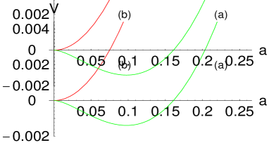
Figure 1: The effective potential of SU(2) QCD in the pure magnetic background. Here (a) is the effective potential and (b) is the classical potential.

Apparently the difference between two effective Lagrangians (13) and (17) follows from different infra-red regularizations. In (13) it was the $\zeta$-function regularization, but in (17) it was the infra-red regularization by causality. Since the $\zeta$-function regularization is such a well established regularization we can not easily dismiss the instability of the monopole condensation. So we have to know which regularization is the correct one, and why. We need an independent method which can settle this controversy.

Fortunately we can settle this controversy with a perturbative method, because the imaginary part of the effective action is of the order of $g^{2}$. The idea that one can actually settle this controversy with a perturbative method was first proposed by Schanbacher sch , but this idea has never been tested by actual calculation before. So we first demonstrate that in massless QED one can indeed calculate the imaginary part perturbatively, and apply the perturbative method to obtain the imaginary part of the QCD effective action. To do this we review the Schwinger’s perturbative calculation of the QED effective action. In QED Schwinger has obtained the following effective action perturbatively to the order $e^{2}$ schw

$$\Delta S_{QED}=\displaystyle\frac{e^{2}}{16\pi^{2}}\int d^{4}pF_{\mu\nu}(p)F_{\mu\nu}(-p)$$

$$\times\displaystyle\frac{}{}\int_{0}^{1}dv\displaystyle\frac{v^{2}(1-v^{2}/3)}{(1-v^{2})+4m^{2}/p^{2}},$$ (20)

where $m$ is the electron mass. From this he observed that when $-p^{2}>4m^{2}$ the integrand develops a pole at $v^{2}=1+4m^{2}/p^{2}$ which generates an imaginary part, and explained how to calculate the imaginary part of the effective action. But notice that in the massless limit, the pole moves to $v=1$. In this case the pole contribution to the imaginary part is reduced by a half, and we obtain

$$Im~{}{\cal L}_{QED}{\Big{|}}_{m=0}=\left\{{~{}0~{}~{}~{}~{}~{}~{}~{}~{}~{}~{}~{}~{}~{}~{}b=0,\atop\displaystyle\frac{b^{2}}{48\pi}~{}~{}~{}~{}~{}~{}~{}~{}~{}~{}~{}a=0.}\right.$$ (21)

Remarkably, this is exactly what we obtain from the non-perturbative effective action in the massless limit cho01prl ; cho01 . This confirms that in massless QED, one can calculate the imaginary part of the effective action either perturbatively or non-perturbatively, with identical results.

Now we repeat the perturbative calculation for QCD. We can do this either by calculating the one-loop Feynman diagrams directly, or by evaluating the integral (12) perturbatively to the order $g^{2}$. We start with the Feynman diagrams. For an arbitrary background $B_{\mu}$ there are four Feynman diagrams that contribute to the order $g^{2}$ which are shown in Fig. 2. Notice that the tadpole diagrams contain a quadratic divergence which does not appear in the final result.

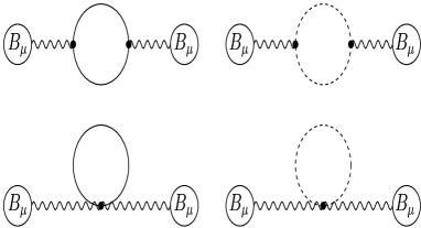
Figure 2: The Feynman diagrams that contribute to the effective action at $g^{2}$ order. Here the straight line and the dotted line represent the valence gluon and the ghost, respectively.

The sum of these diagrams (in the Feynman gauge with dimensional regularization) gives us pesk

$$\Delta S=-\displaystyle\frac{11g^{2}}{96\pi^{2}}\int d^{4}pG_{\mu\nu}(p)G_{\mu\nu}(-p)$$

$$\times\left[\mbox{ln}\left(\displaystyle\frac{p^{2}}{\mu^{2}}\right)+C_{1}\right],$$ (22)

where $C_{1}$ is a regularization-dependent constant. Clearly the imaginary part could only arise from the term $\mbox{ln}(p^{2}/\mu^{2})$, so that for a space-like $p^{2}$ (with $\mu^{2}>0$) the effective action has no imaginary part. However, since a space-like $p^{2}$ corresponds to a magnetic background, we find that the magnetic condensation generates no imaginary part, at least at the order $g^{2}$. To evaluate the imaginary part for a constant electric background we have to make the analytic continuation of (Stability of Monopole Condensation in SU(2) QCD) to a time-like $p^{2}$, because the electric background corresponds to a time-like $p^{2}$. In this case the causality (with the familiar Feynman prescription $p^{2}\rightarrow p^{2}-i\epsilon$) dictates us to have

$$\mbox{ln}\Big{(}\displaystyle\frac{p^{2}}{\mu^{2}}\Big{)}\rightarrow\lim_{\epsilon\to 0}\mbox{ln}\Big{(}\displaystyle\frac{p^{2}-i\epsilon}{\mu^{2}}\Big{)}$$

$$=\mbox{ln}\Big{(}\displaystyle\frac{|p^{2}|}{\mu^{2}}\Big{)}-i\displaystyle\frac{\pi}{2}~{}~{}~{}~{}~{}(p^{2}<0),$$ (23)

so that we obtain

$$Im~{}\Delta{\cal L}=\left\{{~{}~{}~{}~{}0~{}~{}~{}~{}~{}~{}~{}~{}~{}~{}~{}~{}(b=0),\atop-\displaystyle\frac{11b^{2}}{96\pi}~{}~{}~{}~{}~{}~{}~{}~{}~{}(a=0).}\right.$$ (24)

This allows us to conclude that the result (17) is indeed endorsed by the Feynman diagram calculation.

To remove any lingering doubt about (17) we now make the perturbative calculation of the integral (12) to the order $g^{2}$ with the Schwinger’s method, and find hon

$$\Delta S=-\displaystyle\frac{g^{2}}{8\pi^{2}}\int d^{4}pG_{\mu\nu}(p)G_{\mu\nu}(-p)\Sigma(p),$$

$$\Sigma(p)=\displaystyle\frac{}{}\int_{0}^{1}dv(1-\displaystyle\frac{v^{2}}{4})\displaystyle\frac{}{}\int_{0}^{\infty}\displaystyle\frac{dt}{t}\exp[-\displaystyle\frac{p^{2}}{4}(1-v^{2})t]$$

$$=2\displaystyle\frac{}{}\int_{0}^{1}dv\displaystyle\frac{v^{2}(1-v^{2}/12)}{1-v^{2}}+C_{2},$$ (25)

where $C_{2}$ is a regularization-dependent constants. Now, it is straightforward to evaluate the imaginary part of $\Delta S$. Comparing this with Schwinger’s result (20) for the massless QED we again reproduce (24), after the proper charge and wave function renormalization.

Furthermore, from the definition of the exponential integral function table

$$Ei(-z)=-\displaystyle\frac{}{}\int_{z}^{\infty}\displaystyle\frac{d\tau}{\tau}\exp(-\tau)=\gamma+\mbox{ln}z$$

$$+\displaystyle\frac{}{}\int_{0}^{z}\displaystyle\frac{d\tau}{\tau}\left[\exp(-\tau)-1\right]~{}~{}~{}({\rm Re}~{}z>0),$$ (26)

we can express $\Sigma(p)$ as

$$\Sigma(p)=-\displaystyle\frac{}{}\lim_{\epsilon\to 0}\int_{0}^{1}dv(1-\displaystyle\frac{v^{2}}{4})\left[\gamma+\mbox{ln}\Big{(}\displaystyle\frac{p^{2}}{4\mu^{2}}(1-v^{2})\epsilon\Big{)}\right]$$

$$=\displaystyle\frac{11}{12}\left[\mbox{ln}\left(\displaystyle\frac{p^{2}}{\mu^{2}}\right)+C_{3}\right],$$ (27)

where $C_{3}$ is another regularization-dependent constant. This tells that (25) is identical to (Stability of Monopole Condensation in SU(2) QCD). This is the reason why the perturbative calculation by Feynman diagrams and by Schwinger’s method produce the same result. This strongly indicates that the monopole condensation indeed describes a stable vacuum, but the electric background creates the pair-annihilation of the valence gluons in $SU(2)$ QCD cho02 ; cho99 .

It is striking that both the infra-red regularization by causality and the perturbative method endorse the stability of the monopole condensation. But in retrospect one should not be surprised by this. Remember that the instability of SNO vacuum originates from the tachyonic modes which violate the causality. In physics the appearence of tachyonic modes has always implied that something is wrong in the formalism, and one corrects this defect by introducing a physical condition which can exclude the tachyonic modes. This is what happens in string theory and in spontaneously broken gauge theory. And in QCD obviously the causality is what we need to exclude the unphysical tachyonic modes. So it is natural that both the perturbative method and the infra-red regularization by causality ensure the stability of the monopole condensation in QCD, because both are based on the causality.

This does not mean that the $\zeta$-function regularization has any intrinsic defect. We emphasize that the problem is the incorrect inclusion of the unphysical tachyonic modes in the integral (12), not the $\zeta$-function regularization. The $\zeta$-function regularization is simply too honest to remove the tachyonic modes.

In this paper we have neglected the quarks. We simply remark that the quarks, just as in asymptotic freedom wil , tend to destabilize the monopole condensation. In fact the stability puts exactly the same constraint on the number of quarks as the asymptotic freedom cho99 ; cho1 .

Recently the monopole condensation has been establshed in a supersymmetric generalization of QCD witt . Our analysis tells that one can establsh the magnetic condensation within the framework of QCD, with the existing principles of quantum field theory. It is truly remarkable (and surprising) that the principles of quantum field theory allow us to demonstrate the magnetic condensation, and by implication the confinement of color, within the framework of QCD. This should be interpreted as a most spectacular triumph of quantum field theory itself.

We conclude with the following remarks:
1) We emphasize that the above perturbative calculation of the imaginary part of the one-loop effective action was possible because in QCD (and in massless QED) the imaginary part of the one-loop effective action is of the order $g^{2}$. This assures us that one can make a perturbative expansion for the imaginary part of the effective action. For massive QED, for example, this calculation does not make sense because the imaginary (as well as the real) part of the effective action simply does not allow a convergent perturbative expansion cho01prl ; cho01 . The same argument applies to the real part of QCD. Only for the imaginary part of the massless gauge theories one can make sense out of the perturbative calculation.
2) One might worry about the negative signature of the imaginary part in the QCD effective action. To understand the origin of this, compare QCD with massless QED. The difference between the two is that in QED we have the electron loop, but in QCD we have the valence gluon loop. Obviously they have the opposite statistics (aside from the different kinematic factors which do not change the signature). This is the reason for the negative signature cho02 ; cho99 . This implies that the electric background generates pair-annihilation (not pair-creation) of gluons in QCD. And this is what we need to explain the infra-red slavery, because the pair-annihilation implies the anti-screeing of color. This tells that the negative signature is consistent with the confinement of color.
3) In this paper we have considered only the pure magnetic or pure electric background, so the above result guarantees only the stability of the monopole condensation. To show that this is the true vacuum of QCD, we must calculate the effective action with an arbitrary background. Fortunately, one can actually do this with an arbitrary constant background, and show that indeed the monopole condensation becomes the true vacuum of $SU(2)$ QCD, at least at one-loop level cho99 ; cho1 .

The details of our analysis will be published elsewhere cho2 .

One of the authors (YMC) thanks Professor S. Adler, Professor F. Dyson, and Professor C. N. Yang for the illuminating discussions. The work is supported in part by the Basic Research Program (Grant R02-2003-000-10043-0) of Korea Science and Engineering Foundation and by the BK21 project of Ministry of Education.

References

- (1) Y. Nambu, Phys. Rev. D10, 4262 (1974); S. Mandelstam, Phys. Rep. 23C, 245 (1976); A. Polyakov, Nucl. Phys. B120, 429 (1977); G. ’t Hooft, Nucl. Phys. B190, 455 (1981).
- (2) Y. M. Cho, Phys. Rev. D21, 1080 (1980); Y. M. Cho, Phys. Rev. Lett. 46, 302 (1981); Phys. Rev. D23, 2415 (1981).
- (3) G. K. Savvidy, Phys. Lett. B71, 133 (1977).
- (4) N. Nielsen and P. Olesen, Nucl. Phys. B144, 485 (1978); B160, 380 (1979); C. Rajiadakos, Phys. Lett. B100, 471 (1981).
- (5) A. Yildiz and P. Cox, Phys. Rev. D21, 1095 (1980); M. Claudson, A. Yilditz, and P. Cox, Phys. Rev. D22, 2022 (1980); S. Adler, Phys. Rev. D23, 2905 (1981); W. Dittrich and M. Reuter, Phys. Lett. B128, 321, (1983); C. Flory, Phys. Rev. D28, 1425 (1983); S. K. Blau, M. Visser, and A. Wipf, Int. J. Mod. Phys. A6, 5409 (1991); M. Reuter, M. G. Schmidt, and C. Schubert, Ann. Phys. 259, 313 (1997).
- (6) M. Consoli and G. Preparata, Phys. Lett. B154, 411 (1985); L. Maiani, G. Martinelli, G. Rossi, and M. Testa, Nucl. Phys. B273,275 (1986).
- (7) Y. M. Cho, H. W. Lee, and D. G. Pak, Phys. Lett. B 525, 347 (2002); Y. M. Cho and D. G. Pak, Phys. Rev. D65, 074027 (2002).
- (8) Y. M. Cho and D. G. Pak, in Proceedings of TMU-Yale Symposium on Dynamics of Gauge Fields, edited by T. Appelquist and H. Minakata (Universal Academy Press, Tokyo) (1999); J. Korean Phys. Soc. 38, 151 (2001).
- (9) Y. M. Cho and D. G. Pak, Phys. Rev. Lett. 86, 1947 (2001); D. Lamm, S. Valluri, U. Jentschura, and E. Weniger, Phys. Rev. Lett. 88, 089101 (2002); Y. M. Cho and D. G. Pak, Phys. Rev. Lett. 91, 039101 (2003).
- (10) W. S. Bae, Y. M. Cho, and D. G. Pak, Phys. Rev. D64, 017303 (2001); Y. M. Cho and D. G. Pak, hep-th/0010073.
- (11) V. Schanbacher, Phys. Rev. D26, 489 (1982).
- (12) Y. M. Cho, Phys. Rev. D62, 074009 (2000); W. S. Bae, Y. M. Cho, and S. W. Kimm, Phys. Rev. D65, 025005 (2002).
- (13) Y. M. Cho, Phys. Rev. Lett. 44, 1115 (1980); Phys. Lett. B115, 125 (1982).
- (14) J. Schwinger, Phys. Rev. 82, 664 (1951).
- (15) See for example, C. Itzikson and J. Zuber, Quantum Field Theory (McGraw-Hill) 1985; M. Peskin and D. Schröeder, An Introduction to Quantum Field Theory (Addison-Wesley) 1995; S. Weinberg, Quantum Theory of Fields (Cambridge Univ. Press) 1996.
- (16) A similar result has been obtained by Honerkamp. See J. Honerkamp, Nucl. Phys. B48, 269 (1972).
- (17) See, for example, I. Gradshteyn and I. Ryzhik, Table of Integrals, Series, and Products, edited by A. Jeffery (Academic Press) 1994; M. Abramowitz and I. Stegun, Handbook of Mathematical Functions, (Dover) 1970.
- (18) D. Gross anf F. Wilczek, Phys. Rev. Lett. 26, 1343 (1973); H. Politzer, Phys. Rev. Lett. 26, 1346 (1973).
- (19) Y. M. Cho, hep-th/0006051; hep-th/0301013.
- (20) N. Seiberg and E. Witten, Nucl. Phys. B426, 19 (1994); B431, 484 (1994).
- (21) Y. M. Cho, D. G. Pak, and M. L. Walker, JHEP 05, 073 (2004).