A Three-Family Standard-like Orientifold Model:
Yukawa Couplings and Hierarchy

Abstract

We discuss the hierarchy of Yukawa couplings in a supersymmetric three family Standard-like string Model. The model is constructed by compactifying Type IIA string theory on a $Z_{2}\times Z_{2}$ orientifold in which the Standard Model matter fields arise from intersecting D6-branes. When lifted to M theory, the model amounts to compactification of M-theory on a $G_{2}$ manifold. While the actual fermion masses depend on the vacuum expectation values of the multiple Higgs fields in the model, we calculate the leading worldsheet instanton contributions to the Yukawa couplings and examine the implications of the Yukawa hierarchy.

I Introduction

The basic premise of string phenomenology is to explore the constructions and the particle physics implications of four-dimensional string solutions with phenomenologically viable features (i.e., solutions which give rise to an effective theory containing the Standard Model). The moduli space of different compactifications of string theory is highly degenerate at the perturbative level, and so we are faced with the poorly understood question of how the string vacuum describing the observable world is selected. Nevertheless, by exploring models with quasi-realistic features from various corners of M theory, one may deduce some generic physical implications of string derived models.

Prior to the second string revolution, the focus of string phenomenology was on the construction of such solutions within the framework of the weakly coupled heterotic string. Over the years, many semi-realistic models have been constructed in this framework, and the resulting phenomenology has been subsequently analysed [1]. The richness of semi-realistic heterotic string models is also in sharp contrast to the apparent no-go theorem in other formulations of string theory [2]. More recently, the techniques of conformal field theory in describing D-branes and orientifold planes allow for the construction of quasi-realistic string models in another calculable regime of M theory, as illustrated by the various four-dimensional $N=1$ supersymmetric Type II orientifolds[3, 4, 5, 6, 7, 8, 9, 10, 11, 12, 13, 14]. In these models, chiral fermions appear on the worldvolume of the D-branes since they are located at orbifold singularities in the internal space.

Another promising direction to obtain chiral fermions, which has only recently been exploited in model building, is to consider branes at angles. The spectrum of open strings stretched between branes at angles may contain chiral fermions which are localized at the intersection of branes [15]. This fact (or its T-dual version, i.e., branes with flux) was employed in [16, 17, 18, 19, 20, 21, 22, 23, 24] in constructing semi-realistic brane world models. However, the semi-realistic models considered in this context are typically non-supersymmetric, and the stability of non-supersymmetric models (and the dynamics involved in restabilization) is not fully understood. This was one of the motivations of [25, 26, 27] in constructing chiral supersymmetric orientifold models with branes at angles. The constraints on supersymmetric four-dimensional models are rather restrictive. Despite the remarkable progress in developing techniques of orientifold constructions, there is only one orientifold model [25, 26, 27] that has been constructed so far with the ingredients of the MSSM : ${\cal N}=1$ supersymmetry, the Standard Model gauge group as a part of the gauge structure, and candidate fields for the three generations of quarks and leptons as well as the electroweak Higgs doublets.

The general class of supersymmetric orientifold models considered in [25, 26, 27] corresponds (in the strong coupling limit) to M theory compactification on purely geometrical backgrounds admitting a $G_{2}$ metric, providing the first explicit realization of M theory compactification on compact $G_{2}$ holonomy spaces that yields non-Abelian gauge groups and chiral fermions as well as other quasi-realistic features of the Standard and GUT models. This work also sheds light on the recent results of obtaining four-dimensional chiral fermions from $G_{2}$ compactifications of M theory [28, 29, 30, 25, 26], as further elaborated in [27].

In this paper, we further explore the basic properties of the models, in particular the three-family Standard-like Model in [25, 26]. The construction, the chiral spectrum and some of the basic features of the model were described in the original work [25, 26]. The details of the chiral and non-chiral spectra, the explicit evaluation of the gauge couplings, the properties of the two extra $U(1)^{\prime}$ symmetries, and further phenomenological implications associated with charge confinement in the strongly coupled quasi-hidden sector were discussed in [31].

The model is not fully realistic. In addition to the Standard Model group, there are two additional $U(1)^{\prime}$ symmetries, one of which has family non-universal and therefore flavor changing couplings, and a quasi-hidden non-abelian sector which becomes strongly coupled above the electroweak scale. The perturbative spectrum contains a fourth family of exotic ($SU(2)$- singlet) quarks and leptons, in which, however, the left-chiral states have unphysical electric charges. In [31] it is argued that these could decouple from the low energy spectrum due to hidden sector charge confinement, and that anomaly matching requires the physical left-chiral states to be composites. The model has multiple Higgs doublets and additional exotic states. The low energy predictions for the gauge couplings depend on the choice moduli parameters. The study in [31] reveals that $\alpha_{strong}$ can be fitted to the experimental value, while $\sin^{2}\theta_{W}$ and $\alpha_{EM}$ are off by about a factor of $2$ and $3$, respectively.

The purpose of this paper is to carry out further the analysis of the couplings in the model. In particular, we focus on the calculation of Yukawa couplings and study their physical implications. The Yukawa couplings among chiral matter are due to the world-sheet instanton contributions associated with the action of string world-sheet stretching among intersections where the corresponding chiral matter fields are located. The leading contribution to the Yukawa couplings is therefore proportional to $\exp(-A/(2\pi\alpha^{\prime}))$ where $A$ is the smallest area of the string world-sheet stretching among the brane intersection points. The complete calculation of the Yukawa couplings involves techniques of calculating correlation functions involving twisted fields in the conformal field theory of open strings. The origin of the Yukawa couplings, i.e., their world-sheet instanton origin and the consequences of the exponential hierarchies within interesecting brane constructions, was first discussed and analyzed in [17]. (For related applications to the fermion mass hierarchy within GUT intersecting brane constructions, see [32].)

The purpose of our work is to systematically evaluate the leading order contributions to the Yukawa couplings for the supersymmetric three family Standard-like model. Even though we will approach the study only in the leading order of world-sheet instanton contributions, we shall elucidate these features explicitly and discuss the consequences of the resulting hierarchies of the Yukawa couplings. The method can also be further applied to other constructions involving intersecting branes.

The structure of the paper is as follows. In section 2 we briefly describe the features of the model and the chiral spectrum. In section 3 we focus on the calculation of the Yukawa couplings both in the quark and lepton sectors of the model. In section 4 we discuss some physical implications of the hierarchical structure of these couplings and other possible low energy implications. The conclusions are given in section 5.

II Brief Description of the Model

The model is an orientifold of type IIA on ${\bf T}^{6}/({\bf Z}_{2}\times{\bf Z}_{2})$. The orbifold actions have generators $\theta$, $\omega$ acting as $\theta:(z_{1},z_{2},z_{3})\to(-z_{1},-z_{2},z_{3})$, and $\omega:(z_{1},z_{2},z_{3})\to(z_{1},-z_{2},-z_{3})$ on the complex coordinates $z_{i}$ of ${\bf T}^{6}$, which is assumed to be factorizable. The orientifold action is $\Omega R$, where $\Omega$ is world-sheet parity, and $R$ acts by $R:\ (z_{1},z_{2},z_{3})\to({\overline{z}}_{1},{\overline{z}}_{2},{\overline{z}}_{3})$. The model contains four kinds of O6-planes, associated with the actions of $\Omega R$, $\Omega R\theta$, $\Omega R\omega$, $\Omega R\theta\omega$. The cancellation of the RR crosscap tadpoles requires an introduction of $K$ stacks of $N_{a}$ D6-branes ($a=1,\ldots,K$) wrapped on three-cycles (taken to be the product of 1-cycles $(n_{a}^{i},m_{a}^{i})$ in the $i^{th}$ two-torus), and their images under $\Omega R$, wrapped on cycles $(n_{a}^{i},-m_{a}^{i})$. In the case where D6-branes are chosen parallel to the O6-planes, the resulting model is related by T-duality to the orientifold in [4], and is non-chiral. Chirality is however achieved using D6-branes at non-trivial angles.

The cancellation of untwisted tadpoles imposes constraints on the number of D6-branes and the types of 3-cycles that they wrap around. The cancellation of twisted tadpoles determines the orbifold actions on the Chan-Paton indices of the branes (the explicit form of the orbifold actions are given in [25, 26]). The condition that the system of branes preserves ${\cal N}=1$ supersymmetry requires [15] that each stack of D6-branes is related to the O6-planes by a rotation in $SU(3)$: denoting by $\theta_{i}$ the angles the D6-brane forms with the horizontal direction in the $i^{th}$ two-torus, supersymmetry preserving configurations must satisfy $\theta_{1}\,+\,\theta_{2}\,+\,\theta_{3}\,=\,0$. This in turn imposes a constraint on the wrapping numbers and the complex structure moduli $\chi_{i}=R_{2}^{(i)}/R_{1}^{(i)}$, where $R_{1,2}^{(i)}$ are the respective sizes of the $i$-th two-torus.

An example leading to a three-family Standard-like Model massless spectrum corresponds to the following case. The D6-brane configuration is provided in Table I, and satisfies the tadpole cancellation conditions. The configuration is supersymmetric for $\chi_{1}:\chi_{2}:\chi_{3}=1:3:2$.

Type	$N_{a}$	$(n_{a}^{1},m_{a}^{1})\times(n_{a}^{2},m_{a}^{2})\times(n_{a}^{3},\widetilde{m}_{a}^{3})$	Group
$A_{1}$	8	$(0,1)\times(0,-1)\times(2,{\widetilde{0}})$	$Q_{8,8^{\prime}}$
$A_{2}$	2	$(1,0)\times(1,0)\times(2,{\widetilde{0}})$	$Sp(2)_{A}$
$B_{1}$	4	$(1,0)\times(1,-1)\times(1,{\widetilde{3/2}})$	$SU(2)$
$B_{2}$	2	$(1,0)\times(0,1)\times(0,{\widetilde{-1}})$	$Sp(2)_{B}$
$C_{1}$	6+2	$(1,-1)\times(1,0)\times(1,{\widetilde{1/2}})$	$SU(3),Q_{3},Q_{1}$
$C_{2}$	4	$(0,1)\times(1,0)\times(0,{\widetilde{-1}})$	$Sp(4)$

TABLE I.: D6-brane configuration for the three-family model. Here, $\tilde{m}^{3}_{a}=m_{a}^{3}+\frac{1}{2}n_{a}^{3}$.

The rules to compute the spectrum are analogous to those in [18]. Here, we summarize the resulting chiral spectrum in Table II, found in [25, 26], where

$$I_{ab}\ =\ (n_{a}^{1}m_{b}^{1}-m_{a}^{1}n_{b}^{1})(n_{a}^{2}m_{b}^{2}-m_{a}^{2}n_{b}^{2})(n_{a}^{3}m_{b}^{3}-m_{a}^{3}n_{b}^{3})$$ (1)

is the intersection number of $D6_{a}$ and $D6_{b}$ branes [16, 17].

Sector	Representation
$aa$	$U(N_{a}/2)$ vector multiplet
	3 Adj. chiral multiplets
$ab+ba$	$I_{ab}$ chiral multiplets in $(\raisebox{-0.5pt}{\hbox{\rule{0.4pt}{6.5pt}\hskip-0.4pt\rule{6.5pt}{0.4pt}\hskip-6.5pt\rule[6.5pt]{6.5pt}{0.4pt}}\rule[6.5pt]{0.4pt}{0.4pt}\hskip-0.4pt\rule{0.4pt}{6.5pt}}_{a},\overline{\raisebox{-0.5pt}{\hbox{\rule{0.4pt}{6.5pt}\hskip-0.4pt\rule{6.5pt}{0.4pt}\hskip-6.5pt\rule[6.5pt]{6.5pt}{0.4pt}}\rule[6.5pt]{0.4pt}{0.4pt}\hskip-0.4pt\rule{0.4pt}{6.5pt}}}_{b})$ rep.
$ab^{\prime}+b^{\prime}a$	$I_{ab^{\prime}}$ chiral multiplets in $(\raisebox{-0.5pt}{\hbox{\rule{0.4pt}{6.5pt}\hskip-0.4pt\rule{6.5pt}{0.4pt}\hskip-6.5pt\rule[6.5pt]{6.5pt}{0.4pt}}\rule[6.5pt]{0.4pt}{0.4pt}\hskip-0.4pt\rule{0.4pt}{6.5pt}}_{a},\raisebox{-0.5pt}{\hbox{\rule{0.4pt}{6.5pt}\hskip-0.4pt\rule{6.5pt}{0.4pt}\hskip-6.5pt\rule[6.5pt]{6.5pt}{0.4pt}}\rule[6.5pt]{0.4pt}{0.4pt}\hskip-0.4pt\rule{0.4pt}{6.5pt}}_{b})$ rep.
$aa^{\prime}+a^{\prime}a$	$-\frac{1}{2}(I_{aa^{\prime}}-\frac{4}{2^{k}}I_{a,O6})$ chiral multiplets in            rep.
	$-\frac{1}{2}(I_{aa^{\prime}}+\frac{4}{2^{k}}I_{a,O6})$ chiral multiplets in            rep.

TABLE II.: General spectrum on D6-branes at generic angles (namely, not parallel to any O6-plane in all three tori). The spectrum is valid for tilted tori. The models may contain additional non-chiral pieces in the $aa^{\prime}$ sector and in $ab$, $ab^{\prime}$ sectors with zero intersection, if the relevant branes overlap.

Sector	$SU(3)\times SU(2)\times Sp(2)_{B}\times Sp(2)_{A}\times Sp(4)$	$Q_{3}$	$Q_{1}$	$Q_{2}$	$Q_{8}$	$Q_{8}^{\prime}$	$Q_{Y}$	$Q_{8}-Q_{8}^{\prime}$	Field
$A_{1}B_{1}$	$3\times 2\times(1,{\overline{2}},1,1,1)$	0	0	$-1$	$\pm 1$	0	$\pm\frac{1}{2}$	$\pm 1$	$H_{U}$, $H_{D}$
	$3\times 2\times(1,{\overline{2}},1,1,1)$	0	0	$-1$	0	$\pm 1$	$\pm\frac{1}{2}$	$\mp 1$	$H_{U}$, $H_{D}$
$A_{1}C_{1}$	$2\times(\overline{3},1,1,1,1)$	$-1$	0	0	$\pm 1$	0	$\frac{1}{3},-\frac{2}{3}$	$1,-1$	$\bar{D}$, $\bar{U}$
	$2\times(\overline{3},1,1,1,1)$	$-1$	0	0	0	$\pm 1$	$\frac{1}{3},-\frac{2}{3}$	$-1,1$	$\bar{D}$, $\bar{U}$
	$2\times(1,1,1,1,1)$	0	$-1$	0	$\pm 1$	0	$1,0$	$1,-1$	$\bar{E}$, $\bar{N}$
	$2\times(1,1,1,1,1)$	0	$-1$	0	0	$\pm 1$	$1,0$	$-1,1$	$\bar{E}$, $\bar{N}$
$B_{1}C_{1}$	$(3,{\overline{2}},1,1,1)$	1	0	$-1$	0	0	$\frac{1}{6}$	0	$Q_{L}$
	$(1,{\overline{2}},1,1,1)$	0	1	$-1$	0	0	$-\frac{1}{2}$	0	$L$
$B_{1}C_{2}$	$(1,2,1,1,4)$	0	0	$1$	0	0	0	0
$B_{2}C_{1}$	$(3,1,2,1,1)$	1	0	0	0	0	$\frac{1}{6}$	0
	$(1,1,2,1,1)$	0	1	0	0	0	$-\frac{1}{2}$	0
$B_{1}C_{1}^{\prime}$	$2\times(3,2,1,1,1)$	1	0	1	0	0	$\frac{1}{6}$	0	$Q_{L}$
	$2\times(1,2,1,1,1)$	0	1	1	0	0	$-\frac{1}{2}$	0	$L$
$B_{1}B_{1}^{\prime}$	$2\times(1,1,1,1,1)$	0	0	$-2$	0	0	0	0
	$2\times(1,3,1,1,1)$	0	0	$2$	0	0	0	0
$A_{1}A_{1}$	$3\times 8\times(1,1,1,1,1)$	0	0	0	0	0	0	0
	$3\times 4\times(1,1,1,1,1)$	0	0	0	$\pm 1$	$\pm 1$	$\pm 1$	0
	$3\times 4\times(1,1,1,1,1)$	0	0	0	$\pm 1$	$\mp 1$	0	$\pm 2$
	$3\times(1,1,1,1,1)$	0	0	0	$\pm 2$	0	$\pm 1$	$\pm 2$
	$3\times(1,1,1,1,1)$	0	0	0	0	$\pm 2$	$\pm 1$	$\mp 2$
$A_{2}A_{2}$	$3\times(1,1,1,1,1)$	0	0	0	0	0	0	0
$B_{1}B_{1}$	$3\times(1,3,1,1,1)$	0	0	0	0	0	0	0
	$3\times(1,1,1,1,1)$	0	0	0	0	0	0	0
$B_{2}B_{2}$	$3\times(1,1,1,1,1)$	0	0	0	0	0	0	0
$C_{1}C_{1}$	$3\times(8,1,1,1,1)$	0	0	0	0	0	$0$	0
	$3\times(1,1,1,1,1)$	0	0	0	0	0	$0$	0
$C_{2}C_{2}$	$3\times(1,1,1,1,5+1)$	0	0	0	0	0	0	0

TABLE III.: The chiral spectrum of the open string sector in the three-family model. To be complete, we also list (in the bottom part of the table, below the double horizontal line) the chiral states from the $aa$ sectors, which are not localized at the intersections.

The chiral spectrum is given in Table III (see [25]). Here, we list also the chiral matter from the $aa$ sectors. The charges of the matter fields under various $U(1)$ gauge fields of the model are tabulated. The generators $Q_{3}$, $Q_{1}$ and $Q_{2}$ refer to the $U(1)$ factor within the corresponding $U(n)$, while $Q_{8}$, $Q_{8}^{\prime}$ are the $U(1)$’s arising from Higgsing the $USp(8)$. The last column provides the charges under a particular anomaly-free $U(1)$ gauge field:

$$Q_{Y}=\frac{1}{6}Q_{3}-\frac{1}{2}Q_{1}+\frac{1}{2}\left(Q_{8}+Q_{8}^{\prime}\right)$$ (2)

This linear combination $Q_{Y}$ plays the role of hypercharge. There are two additional non-anomalous $U(1)$ symmetries, i.e., $\frac{1}{3}Q_{3}-Q_{1}$ and $Q_{8}-Q_{8}^{\prime}$. The spectrum of chiral multiplets corresponds to three quark-lepton generations, a number of vector-like Higgs doublets, and an anomaly-free set of chiral matter. It includes states corresponding to the right-handed $SU(2)$-singlet fields of a fourth family. However, their natural left-handed partners, from the $B_{2}C_{1}$ sector, have the wrong hypercharge. It is argued in [31] that these disappear from the low energy spectrum due to the strong coupling of the first $Sp(2)$ group, to be replaced by composites with the appropriate quantum numbers to be the partners of the extra family of right-handed fields.

The gauge couplings of the various gauge fields in the model (determined by the volume of the 3-cycles that the corresponding D6-brane wraps around [25]) were calculated explicitly in [31]. In this paper we shall focus on the Yukawa couplings.

III Yukawa Couplings

In this section we calculate the leading contribution to the Yukawa couplings among the chiral matter fields in the model. The string theory calculation of the Yukawa couplings requires the techniques of computing string amplitudes that involve twisted fields of the conformal field theory describing the open strings states at each intersection. In particular, the quantization of the open string sector associated with the string states at the interection of two D-branes at a general angle $\theta$ involves states with the boundary conditions that are a linear combination of Dirichlet and Neumann boundary conditions. Thus the mode expansion is in terms of $\alpha_{n-k}$ modes and the non-integer powers of the world-sheet coordinate $z\equiv{\rm exp}(\tau+i\sigma)$, i.e., $X^{i}\sim\sum_{n}{{\alpha_{n-k}^{i}}\over{n-k}}\,z^{-(n-k)}$, where $n$ are integers, and $k={\theta\over{2\pi}}$. Therefore states in this sector are created by acting with $\alpha_{n-k}$ ($n-k<0$) on the “twisted” vacuum $\sigma_{k}|\,0\,\rangle$, where $\sigma_{k}$ is the conformal field that ensures the correct boundary conditions on the open string states. As a consequence the string amplitude for the three states, each of them at an intersection of two D-branes where the three intersections form the edges of a triangle, involves a calculation of a correlator of the type $\langle\,0\,|\partial_{z}X^{i_{1}}\,\partial_{z}X^{i_{2}}\,\partial_{z}X^{i_{3}}\,\sigma_{k_{1}}\,\sigma_{k_{2}}\,\sigma_{k_{3}}\,|\,0\,\rangle$ (with $\sum_{i=1}^{3}k_{i}=1$). [The fermionic sector of the correlator can be determined in a straightforward way by employing the bosonisation procedure of the world-sheet fermionic degrees of freedom.] Since each state is localized at the intersection of the D-branes, this amplitude involves the contribution of the worldsheet instantons, and it is thus exponentially suppressed by the area of the corresponding intersection triangle. The results of the calculation should be analogous to Yukawa coupling calculations for the twisted closed string states of orbifolds [33]. However, the subtleties of the open-string sector calculations (such as the so-called “doubling trick”, that allows one to express the open string modes in terms of the holomorphic world-sheet coordinate $z$, only; $z$ is now defined on the whole complex plane, along with the boundary conditions for states specified on the real line) require further study.

The Yukawa couplings can therefore be expressed as a sum over the worldsheet instantons associated with the action of the string worldsheet stretching among the intersection points where the corresponding chiral matter fields are located. The couplings are schematically of the form: $\sum_{n=1}^{\infty}Z_{n}\exp[-(nc_{n}A)/(2\pi\alpha^{\prime})]$. Here $A$ is the smallest area of the triangle associated with the corresponding brane intersections and $\alpha^{\prime}$ is the string tension, related to the string scale by $M_{s}=(\alpha^{\prime})^{-1/2}$. (The factor $1/(2\pi)$ in the exponents is due to the normalization of the string Nambu-Goto action with the pre-factor $1/(2\pi\alpha^{\prime})$.) The pre-factors $Z_{n}$ and the coefficients $c_{n}$ in the exponents are of ${\cal{O}}(1)$. (The coefficients $c_{n}$ should in principle include the multiplicity factors due to the orbifold and orientifold symmetries.) The leading contribution to the Yukawa couplings is therefore proportional to $Z_{1}\exp[-(c_{1}A)/(2\pi\alpha^{\prime})]$. The world-sheet instanton origin of Yukawa couplings and the implications for hierarchies within interesecting D-branes was originally studied in [17].

At this stage we shall approach the study systematically by studying the leading order contributions, only. Within this context we shall evaluate the intersection areas $A$ explicitly in terms of the moduli of internal tori. Indeed, even in the leading order in the determination of the Yukawa couplings there remains an uncertainty, since $Z_{1}$ and $c_{1}$, which are coefficients of ${\cal O}(1)$, can only be determined by an explicit string calculation. (Note also that the physical values of the Yukawa couplings also depend on the normalization of the kinetic energy terms for the corresponding matter field, which we will not address here either.)

In particular, we shall explore the basic building blocks for the calculation of $A$, by first positioning the branes very close to the symmetric positions in the six-torus. As the next step we shall then explore the consequences for the Yukawa coupling hierarchy when the branes are moved from the symmetric positions.

There are couplings between the $A_{1}B_{1}$, $B_{1}C_{1}^{\prime}$ and $C_{1}^{\prime}A_{1}$ sectors. Since the $C_{1}^{\prime}A_{1}$ sector is the same as $A_{1}^{\prime}C_{1}$, and furthermore, $A_{1}=A_{1}^{\prime}$ (because the $A_{1}$ brane is the same as its own orientifold image), in principle there are non-zero couplings of the form $(A_{1}B_{1})(B_{1}C_{1}^{\prime})(A_{1}C_{1})$, which could give rise to the Yukawa couplings of the two families of quarks and leptons from the $B_{1}C_{1}^{\prime}$ sector (see Table III). The third family has no Yukawa couplings, since the left-handed quarks and leptons in this family arise from the $B_{1}C_{1}$ sector instead, and hence the three-point couplings are not gauge invariant.

The basic ingredients for calculating the intersection areas are given in Figure 1.

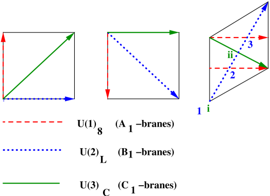
FIG. 1.: The initial symmetric configuration of the $A,B,C^{\prime}$ sectors of branes, associated with the $U(1)_{8,8^{\prime}}$ , $U(2)_{L}$ and $\{U(3)_{C},U(1)_{1}\}$ sectors, are denoted by dashed, dotted, and solid lines, respectively. The intersections denoted by $\alpha=(1,2,3)$ and $\gamma=(i,ii)$ correspond to the appearance of Higgs and left-handed families, respectively.

This is an initial symmetric configuration of the $A,B,C^{\prime}$ sectors of branes, associated with the $U(1)_{8,8^{\prime}}$ , $U(2)_{L}$ and $\{U(3)_{C},U(1)_{1}\}$ sectors, respectively. The set of $A$ branes, associated with $U(1)_{8}$ and $U(1)_{8^{\prime}}$, are positioned very close to the corresponding orientifold plane. (Had they all been positioned exactly on top of the orientifold plane, the gauge group would have been enhanced to $USp(8)$). Thus the couplings associated with the pairs of states that are charged under $U(1)_{8}$ and $U(1)_{8^{\prime}}$, respectively are approximately degenerate. We denote the two sets of Higgs fields with $U(1)_{8}$ charges as $H^{\alpha}_{\{U,D\},\{I,II\}}$ where $\alpha=\{1,2,3\}$. Here, $\alpha$ labels the intersection points of the $A_{1}$ and $B_{1}$ branes (where the Higgs fields are located). The pairs of states denoted by $\{I,II\}$ indices correspond to the two sets of fields appearing at the same intersections. Analogous notation is used for the corresponding right-handed quark and lepton sector. The set of fields associated with $U(1)_{8^{\prime}}$ charges are denoted by $H\to H^{\prime}$ and $\{\bar{U},\bar{D}\}\to\{\bar{U}^{\prime},\bar{D}^{\prime}\}$.

We have also positioned branes associated with $U(3)_{C}$ and $U(1)_{1}$ nearby, which ensures at this stage the near degeneracy of the couplings associated with the quark doublets $Q_{L}^{\gamma}$ and leptons $L_{L}^{\gamma}$ ($\gamma=(i,ii)$) as well as that of the Up- and Down-sector. Due to this large degeneracy, we shall only describe the couplings for the Up-quark sector.

From Figure 1, which depicts the location of the intersections of the $A,B,C^{\prime}$ branes, it is evident that there are different Yukawa couplings associated with the location of the intersections of the two types of left-handed quarks $\gamma=(i,ii)$ and the location of the three types of Higgs fields $H_{U\,\{I,II\}}^{\alpha}$ where $\alpha=1,2,3$ (and $H\to H^{\prime}$ sectors).

While the Higgs fields (and the right-handed quarks) associated with index $I$ and $II$ formally appear at the same intersection, the orientifold and orbifold projection in the construction of these states ensure that only pairs of the Higgs and right-handed quarks with the same $I$ or $II$ index couple to each other.

Thus, in this degenerate case, the Yukawa interactions take the form:

$$H_{yukawa}=\sum_{\alpha,\gamma}h_{\alpha,\,\gamma}Q_{L}^{\gamma}(\bar{U}_{I}H^{\alpha}_{U\,I}+{\bar{U}_{II}}{H}^{\alpha}_{U\,II})\,+(\{\bar{U},H_{U}\}\to\{\bar{U}^{\prime},H_{U}^{\prime}\}),$$ (3)

where $h_{\alpha,\gamma}\sim{\rm exp}(-A_{\alpha,\gamma}/(2\pi\alpha^{\prime}))$.

The area of the triangle associated with the three intersection points (in the six dimensional internal space) can be calculated in terms of the products of the vectors ${\vec{a}}$, ${\vec{b}}$ and ${\vec{c}}$, specifying the respective locations of the three intersections points:

$$Area=\textstyle{1\over 2}|[{\vec{a}}-{\vec{b}}]\times[{\vec{a}}-{\vec{c}}]|=\textstyle{1\over 2}\sqrt{[{\vec{a}}-{\vec{b}}]^{2}[{\vec{a}}-{\vec{c}}]^{2}-\left([{\vec{a}}-{\vec{b}}]\cdot[{\vec{a}}-{\vec{c}}]\right)^{2}}\,.$$ (4)

After these preliminaries we are set to calculate the minimal intersection areas $A_{\alpha,\gamma}$. These can be easily determined from Figure 1, which depicts the position of the building block branes in the fundamental domain of the toroidal lattice, and Figure 2 which depicts the relevant intersection areas for the third toroidal lattice.

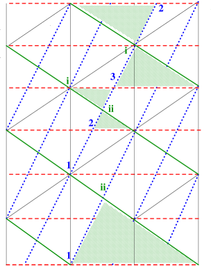
FIG. 2.: Intersection areas of the branes in the third torus. The thin solid lines denote the lattice, the thick solid lines-the $U(3)_{C}$ branes, the dotted lines-$U(2)_{L}$ branes and the dashed ones- $U(1)_{8,8^{\prime}}$ branes. Again $\alpha=(1,2,3)$ and $\gamma=(i,ii)$ denote the location of the three Higgs fields and the two left-handed quark families, respectively.

Employing eq. (4) we obtain the straightforward results for the intersection areas:

$$A_{1,\,i} = 0$$ (5)

$$A_{2,\,i} = A_{3,\,i}=\textstyle{1\over{3}}R_{1}^{(3)}R_{2}^{(3)}$$ (6)

$$A_{2,\,ii} = A_{3,\,ii}=\textstyle{1\over{12}}R_{1}^{(3)}R_{2}^{(3)}$$ (7)

$$A_{1,\,ii} = \textstyle{3\over{4}}R_{1}^{(3)}R_{2}^{(3)}$$ (8)

where $R^{(i)}_{1,2}$ refer to the two sizes of the $i$-th torus, along the $x_{i}$ and $y_{i}$ axis respectively. Note also that $R^{(i)}_{1}R^{(i)}_{2}$ corresponds to the area of the i-th two-torus. Due to the symmetry of the configuration there is no contribution from the area arising from the first two two-tori. We can therefore encounter a sizable hierarchy among different Yukawa couplings. In particular the sub-leading terms $h_{1,ii}$ for $\alpha=1$ are smaller than the couplings for $\alpha=2,3$, as can be seen in (8).

There are phenomenological constraints on the possible values of $R_{1,2}^{(i)}$. The Planck scale and various Yang-Mills couplings are related to the string coupling $g_{s}$ by

$$(M_{P}^{(4d)})^{2}=\frac{M_{s}^{8}V_{6}}{(2\pi)^{7}g_{s}^{2}}\,,$$ (9)

and

$$\frac{1}{g_{YM}^{2}}=\frac{M_{s}^{3}V_{3}}{(2\pi)^{4}g_{s}}\,,$$ (10)

where $V_{6}$ is the volume of the six-dimensional orbifold and $V_{3}$ is the volume of the three-cycle that a specific set of D6-brane wraps. (These volume factors have been explicitly calculated in [31] in terms of the wrapping numbers $(n^{i},m^{i})$ and $R_{1,2}^{(i)}$.)

Using (9) and (10) one can eliminate $g_{s}$ and obtain the relationship between $g_{YM}$, $M_{P}^{4d}$ and $M_{s}$:

$$g_{YM}^{2}M_{P}^{(4d)}=\sqrt{2\pi}M_{s}\frac{\sqrt{V_{6}}}{V_{3}}~{}\,.$$ (11)

For a fixed value of $M_{s}/M_{P}^{(4d)}$, the $g_{YM}$ depend only on the ratios $\frac{\sqrt{V_{6}}}{V_{3}}$, which are functions of the complex structure moduli $\chi_{i}=R^{(i)}_{2}/R^{(i)}_{1}$ only, and have been explicitly evaluated in [31].

Since each gauge group factor of the Standard Model arises from a separate set of branes wrapping a specific three-cycle, there is no internal direction transverse to all the branes. It therefore follows from (9,10,11) that the large Planck scale $M_{P}^{4d}$ cannot be generated by taking any of the internal directions much larger than the inverse of the string scale $M_{s}$, since for perturbative values of the string coupling $g_{s}$ that would make (at least one of) the gauge couplings unrealistic. Thus a large Planck scale is generated from a large string scale and not from a large volume, which is then also compatible with the gauge coupling constraints (10,11). (Note also that experimental bounds on the Kaluza-Klein modes of the Standard Model gauge bosons imply that the extra dimensions cannot be larger than ${\cal O}({\rm TeV}^{-1})$, but this is a much weaker bound than the one obtained by the arguments above.) Finally, the $R_{1,2}^{(i)}$’s cannot be much smaller than the string scale $M_{s}^{-1}$ as this would again make the Planck scale and gauge couplings unrealistic. One should however point out that there still remains some flexibility in adjusting the sizes $R_{1,2}^{(i)}$’s by an order of magnitude or so away from ${\cal O}(M_{s}^{-1})$.

The above constraints that limit generic values of the sizes $R_{1,2}^{(i)}$’s to be close to the inverse of the string scale $M_{s}^{-1}$ (and Planck scale $M_{P}^{4d}$ close to $M_{s}$) have implications for the hierarchy of the Yukawa couplings. Had one had $R_{1,2}^{(i)}\gg M_{s}^{-1}$ the couplings would have been exponentially suppressed. However, since $R_{1,2}^{(i)}={\cal O}(M_{s}^{-1})$, the range dictated from constraints on the Planck scale and gauge couplings, the hierarchy among Yukawa couplings is non-degenerate and may potentially have interesting phenomenological implications. For definiteness, we will require $M_{s}R_{1,2}^{(i)}\geq 2\pi$.

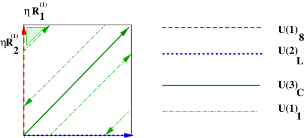
FIG. 3.: The brane configurations in the first torus, depicting the breaking on $U(4)$ Pati-Salam symmetry down to $U(3)_{C}\times U(1)_{1}$. The $U(1)_{1}$ branes (denoted by dash-dotted line) are positioned in a $Z_{2}$ symmetric way relative to $U(3)_{C}$ branes (denoted by a solid line). The separation between them is $\eta R_{1,2}^{(1)}$ in the respective $x$- and $y$-directions. The relevant interesection area in the first torus, contributing to the lepton Yukawa coupling is denoted by a shaded area. [$U(2)_{L}$ and $U(1)_{8,8^{\prime}}$ branes are denoted by a dotted and a dashed line, respectively.]

A Lepton-Quark Splitting

The eight $C_{1}$-branes are split in sets of six and two, thus ensuring the breakdown of $U(4)$ (Pati-Salam type) symmetry down to $U(3)_{C}$ and $U(1)_{1}$. We chose to split them in the first two-torus, keeping $U(3)_{C}$ along the $Z_{2}$ symmetric position and moving $U(1)_{1}$ branes relative to $U(3)_{C}$ ones by a distance $\eta R^{(1)}_{1,2}$ away in the $x$- and $y$- direction, respectively. (See Figure 3). It now becomes a straightforward exercise to determine the new areas associated with the lepton Yukawa couplings. The areas associated with the lepton Yukawa couplings can be expressed in terms of the areas for the quark Yukawa couplings by

$$A^{lepton}_{\alpha,\,\gamma}=\textstyle{1\over 2}\sqrt{(\eta\,{R^{(1)}_{1}})^{2}\,(\eta\,{R^{(1)}_{2}})^{2}+(\eta\,{R^{(1)}_{1}})^{2}\,{\vec{\cal A}_{\alpha,\,\gamma}}^{2}+(\eta{R^{(1)}_{2}})^{2}\,{\vec{\cal B}_{\alpha,\,\gamma}}^{2}+4{A^{quark}_{\alpha,\,\gamma}}^{2}},$$ (12)

where ${\vec{\cal A}_{\alpha,\,\gamma}}$ and ${\vec{\cal B}_{\alpha,\,\gamma}}$ specify the vectors for the respective $U(1)_{8,8^{\prime}}$ and $U(2)_{L}$ sides of the triangles for the corresponding $(\alpha,\,\gamma)$ intersections (in the third toroidal direction).

The areas (12) for lepton Yukawa couplings are always larger than those of the quark couplings. This formula is valid as long as $\eta$ is less or $\sim 1/2$. The values of ${\vec{\cal A}_{\alpha,\,\gamma}}$ and ${\vec{\cal B}_{\alpha,\,\gamma}}$ are give in Table IV, while $A^{quark}_{\alpha,\,\gamma}$ are listed in eq. (8).

$(\alpha,\gamma)$	${\vec{\cal A}_{\alpha,\,\gamma}}^{2}$	${\vec{\cal B}_{\alpha,\,\gamma}}^{2}$
$(1,i)$	0	0
$(2,i),(3,i)$	$\left(\textstyle{4\over 3}R^{(3)}_{1}\right)^{2}$	$\left(\textstyle{1\over 3}R^{(3)}_{1}\right)^{2}+\left(\textstyle{1\over 2}R^{(3)}_{2}\right)^{2}$
$(2,ii),(3,ii)$	$\left(\textstyle{2\over 3}R^{(3)}_{1}\right)^{2}$	$\left(\textstyle{1\over 6}R^{(3)}_{1}\right)^{2}+\left(\textstyle{1\over 4}R^{(3)}_{2}\right)^{2}$
$(1,ii)$	$\left(2R^{(3)}_{1}\right)^{2}$	$\left(\textstyle{1\over 2}R^{(3)}_{1}\right)^{2}+\left(\textstyle{3\over 4}R^{(3)}_{2}\right)^{2}$

TABLE IV.: The values of ${\vec{\cal A}_{\alpha,\,\gamma}}$ and ${\vec{\cal B}_{\alpha,\,\gamma}}$ for the respective $U(1)_{8,8^{\prime}}$ and $U(2)_{L}$ sides of the intersection triangles in the third torus for various $\alpha$ and $\gamma$.

B Up-Down Yukawa Coupling Splitting

The degeneracy of the Yukawa couplings that are associated with states charged under $U(1)_{8}$ and $U(1)_{8^{\prime}}$ can be removed by splitting the branes associated with the first and second abelian factors from the orientifold plane by a distance $\epsilon_{i}$ and $\epsilon_{i}^{\prime}$ in the $i$-th torus ($i=1,2,3$) (see Figure 4). This in turn provides a mechanism for Up-Down sector splitting.

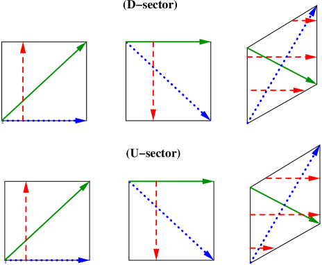
FIG. 4.: The splitting of A-type branes (associated with $U(1)_{8,8^{\prime}}$ and denoted by the dashed lines) from the orientifold planes. For simplicity the figure shows only the fundamental domain of each of the three two-tori. The solid and dotted lines denote the $U(3)_{C}$ and $U(2)_{L}$ branes, respectively.

One can show that the basic ingredients for determining the Up-type [Down-type] Yukawa couplings is to study the intersection of the A-type branes (associated with $U(1)_{8,8^{\prime}}$) moved by a distance $+\epsilon_{i}R^{(i)}_{1}$ [$+\epsilon_{i}R^{(i)}_{1}$] away from the (vertical) orientifold planes in the first two ($i=(1,2)$) two-tori, and a distance $+\epsilon_{3}\,R^{(3)}_{2}$ [$-\epsilon_{3}\,R^{(3)}_{2}$ ] from the (horizontal) orientifold plane in the third torus. Figure 4 depicts these basic displacements of the $A$-type branes in the fundamental domain of each of the two-tori for the Up- and Down-sectors, respectively. In addition, Figures 5 and 6 depict the new $(\alpha,\,\gamma)$ intersection areas in the third toroidal direction for the Up- and Down-sectors, respectively. One can now explicitly calculate the new areas by essentially employing the magnitude of vectors $(\vec{\cal A}_{i})^{2}=(\epsilon_{i}{R^{(i)}_{1}})^{2}$ and $({\vec{\cal B}_{i}})^{2}=(\epsilon_{i}{R^{(i)}_{2}})^{2}$ associated with the sides of the intersection triangles in the first two two-tori for $U(1)_{8,8^{\prime}}$ and $U(2)_{L}$ branes, as well as the corresponding vectors ${\vec{\cal A}_{\alpha,\,\gamma}}$ and ${\vec{\cal B}_{\alpha,\,\gamma}}$ in the respective $U(1)_{8,8^{\prime}}$ and $U(2)_{L}$ sides of the intersection triangles of the third two-torus. For the sake of simplicity we set $\epsilon_{2}=0$, since this significantly simplifies the analytic expression for the intersection area, although the complete formula is straightforward to obtain. The intersection area is:

$$A^{U/D}_{\alpha,\,\gamma}=\textstyle{1\over 2}\sqrt{(\epsilon_{1}{R^{(1)}_{1}})^{2}\,(\epsilon_{1}{R^{(1)}_{2}})^{2}+(\epsilon_{1}{R^{(1)}_{1}})^{2}\,{\vec{\cal A}_{\alpha,\,\gamma}}^{2}+(\epsilon_{1}{R^{(1)}_{2}})^{2}\,{\vec{\cal B}_{\alpha,\,\gamma}}^{2}+4({\tilde{A}}^{U/D}_{\alpha,\,\gamma})^{2}},$$ (13)

where ${\tilde{A}}^{U/D}_{\alpha,\,\gamma}$ refers to the corresponding intersection area in the third toroidal plane. The formula is valid as long as $\epsilon_{1,3}$ are less or $\sim{1\over 2}$. For $U(1)_{8^{\prime}}$ displacements the analogous area formulae are valid with the replacement $\epsilon_{i}\to\epsilon_{i}^{\prime}$.

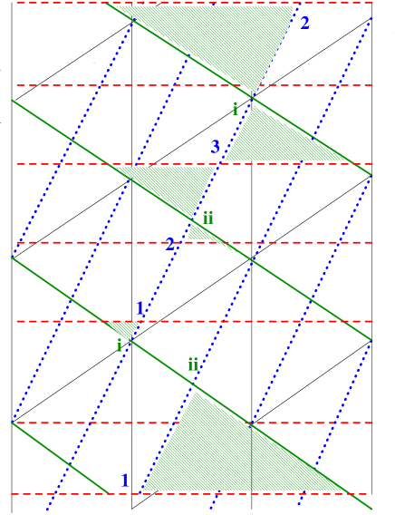
FIG. 5.: Relevant intersection areas in the third toroidal lattice for the Up-sector.

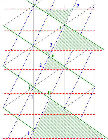
FIG. 6.: Relevant intersection areas in the third toroidal lattice for the Down-sector.

Due to the orbifold and the orientifold symmetries, it is evident from Figures 5 and 6 that a number of Up-Down Yukawa couplings remain degenerate. In particular the following relations hold:

$$A^{U}_{1,\,i} = A^{D}_{1,\,i}$$ (14)

$$A^{U}_{3,\,ii}=A^{D}_{2,\,ii} > A^{U}_{2,\,ii}=A^{D}_{3,\,ii}$$ (15)

$$A^{U}_{2,\,i}=A^{D}_{3,\,i} > A^{U}_{3,\,i}=A^{D}_{2,\,i}$$ (16)

$$A^{U}_{1,\,ii} < A^{D}_{1,\,ii}$$ (17)

Except for the most suppressed Yukawa couplings between the $\alpha=1$ Higgs fields and $\gamma=ii$ quarks, the areas associated with the remaining Up- and Down-Yukawa couplings pair-up.

The explicit values for the areas and the vectors ${\vec{\cal A}_{\alpha\,,\gamma}}$ and ${\vec{\cal B}_{\alpha\,,\gamma}}$ are given in Table V for the Up-sector. In the Up-sector the area for $(3,i)$ is obtained from $(2,i)$ [and $(2,ii)$ from $(3,ii)$] by changing $\epsilon_{3}\to-\epsilon_{3}$. Similarly the Down-sector area for $(1,ii)$ is obtained from the Up-sector area for $(1,ii)$ by changing $\epsilon_{3}\to-\epsilon_{3}$.

$(\alpha,\gamma)$	${\vec{\cal A}_{\alpha,\,\gamma}}^{2}$	${\vec{\cal B}_{\alpha,\,\gamma}}^{2}$	${\tilde{A}}_{\alpha,\,\gamma}$
$(1,i)$	$\left(\textstyle{8\over 3}\epsilon_{3}R^{(3)}_{1}\right)^{2}$	$\left(\textstyle{2\over 3}\epsilon_{3}R^{(3)}_{1}\right)^{2}+\left(\epsilon_{3}R^{(3)}_{2}\right)^{2}$	$\textstyle{4\over 3}\epsilon_{3}^{2}R^{(3)}_{1}R^{(3)}_{2}$
$(2,i)$	$\left(\textstyle{4\over 3}(1+2\epsilon_{3})R^{(3)}_{1}\right)^{2}$	$\left(\textstyle{1\over 3}(1+2\epsilon_{3})R^{(3)}_{1}\right)^{2}+\left(\textstyle{1\over 2}(1+2\epsilon_{3})R^{(3)}_{2}\right)^{2}$	$\textstyle{1\over 3}(1+2\epsilon_{3})^{2}R^{(3)}_{1}R^{(3)}_{2}$
$(3,ii)$	$\left(\textstyle{2\over 3}(1+4\epsilon_{3})R^{(3)}_{1}\right)^{2}$	$\left(\textstyle{1\over 6}(1+4\epsilon_{3})R^{(3)}_{1}\right)^{2}+\left(\textstyle{1\over 4}(1+4\epsilon_{3})R^{(3)}_{2}\right)^{2}$	$\textstyle{1\over{12}}(1+4\epsilon_{3})^{2}R^{(3)}_{1}R^{(3)}_{2}$
$(1,ii)$	$\left(2(1-\textstyle{4\over 3}\epsilon_{3})R^{(3)}_{1}\right)^{2}$	$\left(\textstyle{1\over 2}(1-\textstyle{4\over 3}\epsilon_{3})R^{(3)}_{1}\right)^{2}+\left(\textstyle{3\over 4}(1-\textstyle{4\over 3}\epsilon_{3})R^{(3)}_{2}\right)^{2}$	$\textstyle{3\over 4}(1-\textstyle{4\over 3}\epsilon_{3})^{2}R^{(3)}_{1}R^{(3)}_{2}$

TABLE V.: The values of ${\vec{\cal A}_{\alpha,\,\gamma}}^{2}$, ${\vec{\cal B}_{\alpha,\,\gamma}}^{2}$, and ${\tilde{A}}_{\alpha,\,\gamma}$ for various $\alpha$ and $\gamma$. The results reduce to those in Table IV for $\epsilon_{3}=0$.

IV Implications of the Yukawa Coupling Hierarchy

The basic results for the Yukawa couplings are given in equations (3), (8), (12), and (13). It is difficult to discuss the implications for the fermion masses without a detailed knowledge of the Higgs vacuum expectation values (VEVs), which in turn depend on the details of the soft supersymmetry breaking, the effective $\mu$ terms for the Higgs fields, and the normalization factors of the kinetic energy terms, which have not been determined. As was discussed in [31], the large number of Higgs doublets and the lack of a compelling mechanism to generate effective $\mu$ terms, at least at the perturbative level, are significant drawbacks of the construction. Also, the construction contains a strongly coupled quasi-hidden section, which is a candidate for dynamical supersymmetry breaking, and the detailed study of these phenomena is in progress [34].

Nevertheless, we can make a few general comments about the implications of the Yukawa couplings, emphasizing the simplest case in which the D6 branes are positioned very close to the symmetric positions in the six-torus, as in (8). In this case, there are only four independent Yukawa couplings, $h_{1,i},h_{2,ii}=h_{3,ii},h_{2,i}=h_{3,i}$, and $h_{1,ii}$. As discussed in Section III there are theoretical uncertainties concerning the prefactors and numerical factors in the exponents. For definiteness, we will assume that $h_{\alpha,\gamma}\sim\exp(-A_{\alpha,\gamma}/(2\pi\alpha^{\prime}))$ is a good approximation at least for the ratios of Yukawa couplings. We will also assume that $M_{s}R_{1,2}^{(3)}\geq 2\pi$. In that case, $h_{1,i}\sim 1$, $h_{2,ii}=h_{3,ii}\leq 0.59$, $h_{2,i}=h_{3,i}\leq 0.12$, and $h_{1,ii}\leq 0.009$, with all but $h_{1,i}$ being extremely small for $R_{1,2}^{(3)}$ much larger than the minimum value of $2\pi/M_{s}$. Intermediate values for the $R_{1,2}^{(3)}$ will yield nontrivial hierarchies for the Yukawas.

It is convenient to rewrite (3) as

$$H_{yukawa} = Q_{L}^{i}\sum_{K=1}^{4}\left[h_{1,i}H^{1}_{UK}+\sqrt{2}h_{2,i}\left(\frac{H^{2}_{UK}+H^{3}_{UK}}{\sqrt{2}}\right)\right]\bar{U}_{K}$$ (18)

$$+ Q_{L}^{ii}\sum_{K=1}^{4}\left[h_{1,ii}H^{1}_{UK}+\sqrt{2}h_{2,ii}\left(\frac{H^{2}_{UK}+H^{3}_{UK}}{\sqrt{2}}\right)\right]\bar{U}_{K},$$ (19)

where the index $K$ represents the four terms ($I,II$, and the primed terms) in (3). When some of the Higgs fields acquire VEVs this will yield a $2\times 4$ mass matrix for the two $U$ quarks and four antiquarks. However, in the special case that the two rows are proportional (i.e., that they are aligned in the $K$ direction), there will only be a single nonzero mass eigenvalue. Let us first consider the case of large sizes, so that all of the couplings are small except $h_{1,i}$. Then, there will only be one significant mass term, corresponding to $Q_{L}^{i}$ and a linear combination of the $\bar{U}_{K}$, with coefficients depending on the VEVs of the $H^{1}_{UK}$. The other mass eigenvalue will be exponentially small. In the special case of radiative symmetry breaking, usually associated with supergravity mediated supersymmetry breaking but also occurring for gauge mediation, the second mass would be exactly zero. That is because only the $H^{1}_{UK}$’s have the large Yukawa couplings needed to drive their (presumably positive) mass-squares at the string scale to negative values at low energies, and the VEVs of the other Higgs doublets would vanish. (The small $h_{1,ii}$ would lead to a tiny mixing between $Q^{1}_{L}$ and $Q^{2}_{L}$, but not generate a second non-zero mass because the two terms would be aligned in $K$.) On the other hand, for small $R_{1,2}^{(3)}$ both $h_{1,i}$ and $\sqrt{2}h_{2,ii}$ (the Yukawa coupling for the relevant state $({H^{2}_{UK}+H^{3}_{UK}})/\sqrt{2}$), could be significant, leading to two non-zero mass eigenstates provided that the terms are not aligned in $K$. For radiative breaking, the two large Yukawas could drive both relevant mass-squares negative, and alignment would not be expected except for very specific values for the mass-squares at the string scale and the effective $\mu$ parameters and kinetic terms. In this case, the hierarchy $m_{t}\gg m_{c}$, $m_{u}=0$ could be achieved by a hierarchy in the VEVs of the $H^{1}_{UK}$’s relative to the $({H^{2}_{UK}+H^{3}_{UK}})/\sqrt{2}$), which could be achieved by modest differences in the relevant soft supersymmetry breaking and other terms.

Thus, it is possible to achieve a hierarchy of Up mass eigenvalues, associated with the hierarchy of Yukawa couplings or of VEVs or both. As discussed after (17), even after moving the branes from their symmetric positions the Up and Down Yukawas are the same up to relabelling except for the smallest coupling $h_{1,ii}$. Thus, the hierarchy $m_{t}\gg m_{b}$ would have to come about because the $H^{1}_{UK}$ VEVs are much larger than those for the $H^{1}_{DK}$, analogous to the large $\tan\beta$ region of the MSSM. This can easily occur for moderate differences in the soft mass-squares, especially if the effective $A$ parameters are small. The full hierarchy of $m_{t},m_{b},m_{c},$ and $m_{s}$ (with $m_{d}=m_{u}=0$) could most likely be achieved for appropriate soft and effective $\mu$ parameters and kinetic energy terms, but we do not pursue this in detail since these have not been calculated. Similarly, non-trivial quark mixing could be generated by different $K$ dependence of the VEVs in the $H_{U}$ and $H_{D}$ sectors.

In the symmetric case the charged lepton Yukawas are the same as for the Up and Down quarks, and the charged leptons couple to the same Higgs doublets as the Down quarks. This is analogous to the $t-b-\tau$ Yukawa universality of the simplest version of $SO(10)$ grand unification, which is successful for large $\tan\beta$. (In addition to the $b-\tau$ Yukawa relation at the string scale, one also has $s-\mu$ unification. Of course, the quark Yukawas are enhanced by QCD and other effects in the running down from the string scale, leading to a successful $m_{b}/m_{\tau}$ prediction, but a rather large value for $m_{s}/m_{\mu}$.) The corrections to the lepton Yukawas from moving the $U(1)_{1}$ branes in (12) decrease the lepton Yukawas relative to the symmetric quark couplings, increasing the $m_{b}/m_{\tau}$ prediction. Such a shift is acceptable as long as is small. The $U(1)_{8,8^{\prime}}$ shifts in (13) have the same effects on the leptons as the quarks.

One expects Dirac neutrino masses comparable to the quark and charged lepton masses close to the symmetric points. The possibility of a neutrino seesaw was commented on in [31]. In particular, Majorana masses for the right-handed neutrinos $\bar{N}$ cannot be significantly larger than the scales at which the two additional $U(1)^{\prime}$ factors of the model are broken. It was shown that when the charge confinement and anomaly conditions associated with the strongly coupled quasi-hidden sector are taken into account, then there would be scalar fields with the appropriate quantum numbers to break both $U(1)^{\prime}$s at a high scale at which the interactions become strongly coupled. This could be $10^{15}$ GeV or higher, which could lead to acceptable seesaw mass scales for the neutrinos. However, the actual potential for those fields and their couplings to the $\bar{N}$ states (needed to estimate the actual masses and mixings) would be non-perturbative effects, beyond the scope of this investigation.

V Conclusions

We have considered the Yukawa couplings in a supersymmetric three family Standard-like string Model. In particular, we have calculated the leading order contributions to the world-sheet instantons associated with the action of the string worldsheet stretching among the intersection points corresponding to the chiral matter fields. We considered both the case in which the branes are located very close to symmetric positions in the six-torus, which leads to a high degeneracy of Yukawa couplings, and the consequences of moving some of the branes away from the symmetric positions. In general there is a large hierarchy of Yukawa couplings, which increases exponentially as the sizes of the tori are increased. The actual fermion masses depend on the vacuum expectation values of the Higgs fields, which in turn depend on the supersymmetry breaking and on the effective $\mu$ parameters. There are typically either two or one massive generations of fermions.

- [1] For reviews, see, e.g., B. R. Greene, Lectures at Trieste Summer School on High Energy Physics and Cosmology (1990); F. Quevedo, hep-th/9603074; A. E. Faraggi, hep-ph/9707311; Z. Kakushadze, G. Shiu, S. H. Tye and Y. Vtorov-Karevsky, Int. J. Mod. Phys. A 13, 2551 (1998); G. Cleaver, M. Cvetič, J. R. Espinosa, L. L. Everett, P. Langacker and J. Wang, Phys. Rev. D 59, 055005 (1999), and references therein.
- [2] L. J. Dixon, V. Kaplunovsky and C. Vafa, Nucl. Phys. B 294, 43 (1987); for generalization of this theorem to less than 4 dimensions, see, J. Erler and G. Shiu, Phys. Lett. B 521, 114 (2001).
- [3] C. Angelantonj, M. Bianchi, G. Pradisi, A. Sagnotti and Ya.S. Stanev, Phys. Lett. B 385, 96 (1996).
- [4] M. Berkooz and R.G. Leigh, Nucl. Phys. B 483, 187 (1997).
- [5] Z. Kakushadze and G. Shiu, Phys. Rev. D 56, 3686 (1997); Nucl. Phys. B 520, 75 (1998); Z. Kakushadze, Nucl. Phys. B 512, 221 (1998).
- [6] G. Zwart, Nucl. Phys. B 526, 378 (1998); D. O’Driscoll, hep-th/9801114;
- [7] G. Shiu and S.-H.H. Tye, Phys. Rev. D 58, 106007 (1998).
- [8] Z. Kakushadze, G. Shiu and S. H. Tye, Nucl. Phys. B 533, 25 (1998); Phys. Rev. D 58, 086001 (1998).
- [9] G. Aldazabal, A. Font, L.E. Ibáñez and G. Violero, Nucl. Phys. B 536, 29 (1999).
- [10] Z. Kakushadze, Phys. Lett. B 434, 269 (1998); Phys. Rev. D 58, 101901 (1998); Nucl. Phys. B 535, 311 (1998).
- [11] M. Cvetič, M. Plümacher and J. Wang, JHEP 0004, 004 (2000).
- [12] M. Klein, R. Rabadán, JHEP 0010, 049 (2000).
- [13] G. Aldazabal, L. E. Ibanez, F. Quevedo and A. M. Uranga, JHEP 0008, 002 (2000).
- [14] M. Cvetič, A. M. Uranga and J. Wang, Nucl. Phys. B 595, 63 (2001).
- [15] M. Berkooz, M. R. Douglas and R. G. Leigh, Nucl. Phys. B 480, 265 (1996).
- [16] R. Blumenhagen, L. Görlich, B. Körs and D. Lüst, JHEP 0010, 006 (2000).
- [17] G. Aldazabal, S. Franco, L. E. Ibáñez, R. Rabadán and A. M. Uranga, JMP 42, 3103 (2001); JHEP 0102, 047 (2001).
- [18] R. Blumenhagen, B. Körs and D. Lüst, JHEP 0102, 030 (2001).
- [19] C. Angelantonj, I. Antoniadis, E. Dudas and A. Sagnotti, Phys. Lett. B 489, 223 (2000).
- [20] L. E. Ibáñez, F. Marchesano and R. Rabadán, JHEP 0111, 002 (2001). For generalization to models with an extra at the string scale, see C. Kokorelis, hep-th/0205147.
- [21] S. Förste, G. Honecker and R. Schreyer, Nucl. Phys. B 593, 127 (2001); JHEP 0106, 004 (2001).
- [22] R. Blumenhagen, B. Körs and D. Lüst, T. Ott, Nucl. Phys. B616, 3 (2001).
- [23] D. Bailin, G. V. Kraniotis and A. Love, Phys. Lett. B 530, 202 (2002).
- [24] C. Kokorelis, hep-th/0207234.
- [25] M. Cvetič, G. Shiu and A. M. Uranga, Phys. Rev. Lett. 87, 201801 (2001).
- [26] M. Cvetič, G. Shiu and A. M. Uranga, Nucl. Phys. B 615, 3 (2001).
- [27] M. Cvetic, G. Shiu and A. M. Uranga, hep-th/0111179.
- [28] M. Atiyah and E. Witten, hep-th/0107177.
- [29] E. Witten, hep-th/0108165.
- [30] B. Acharya and E. Witten, hep-th/0109152.
- [31] M. Cvetič, P. Langacker, and G. Shiu, UPR-990-T, hep-ph/0205252.
- [32] C. Kokorelis, hep-th/0203187.
- [33] L. J. Dixon, D. Friedan, E. J. Martinec and S. H. Shenker, Nucl. Phys. B 282, 13 (1987); S. Hamidi and C. Vafa, Nucl. Phys. B 279, 465 (1987).
- [34] M. Cvetič, P. Langacker and J. Wang, work in progress.