Black hole collision with a scalar particle in four, five and seven dimensional anti-de Sitter spacetimes: ringing and radiation

Abstract

In this work we compute the spectra, waveforms and total scalar energy radiated during the radial infall of a small test particle coupled to a scalar field into a $d$-dimensional Schwarzschild-anti-de Sitter black hole. We focus on $d=4,\,5$ and $7$, extending the analysis we have done for $d=3$. For small black holes, the spectra peaks strongly at a frequency $\omega\sim d-1$, which is the lowest pure anti-de Sitter (AdS) mode. The waveform vanishes exponentially as $t\rightarrow\infty$, and this exponential decay is governed entirely by the lowest quasinormal frequency. This collision process is interesting from the point of view of the dynamics itself in relation to the possibility of manufacturing black holes at LHC within the brane world scenario, and from the point of view of the AdS/CFT conjecture, since the scalar field can represent the string theory dilaton, and $4$, $5$, $7$ are dimensions of interest for the AdS/CFT correspondence.

I Introduction

In this we work we extend the analysis we have done for 3-dimensional anti-de Sitter (AdS) lemosvitor , and compute in detail the collision between a black hole and a scalar particle. Now, a charged particle following toward a black hole emits radiation of the corresponding field. Thus, a scalar particle falling into a black hole emits scalar waves. This collision process is interesting from the point of view of the dynamics itself in relation to the possibility of manufacturing black holes at LHC within the brane world scenario dim , and from the point of view of the AdS/CFT conjecture, since the scalar field can represent the string theory dilaton, and $4$, $5$, $7$ (besides $3$) are dimensions of interest for the AdS/CFT correspondence aharonyetal ; HH . In addition, one can compare this process with previous works, since there are results for the quasinormal modes of scalar, and electromagnetic perturbations which are known to govern the decay of the perturbations, at intermediate and late times lemosvitor ; HH ; cardoso3 ; cardosolemos1 .

AdS spacetime is the background spacetime in supersymmetric theories of gravity such as 11-dimensional supergravity and M-theory (or string theory). The dimension $d$ of AdS spacetime is treated as a parameter which, in principle, can have values from two to eleven in accord to these theories, and where the other spare dimensions either receive a Kaluza-Klein treatment or are joined as a compact manifold $\cal M$ into the whole spacetime to yield ${\rm AdS}_{d}\times{\cal M}^{11-d}$. By taking a low energy limits at strong coupling and by performing a group theoretic analysis, Maldacena has conjecture a correspondence between the bulk of $d$-dimenisonal AdS spacetime in string theory and a dual conformal field gauge theory (CFT) on the spacetime boundary maldacenaconjecture . The first system to be studied with care was a D-3brane, in which case the conjecture states that type IIB superstring theory in $AdS_{5}\times S^{5}$ is the same as $\cal N$$=4$ $SU(N)$ super-Yang-Mills (conformal) theory on $S^{3}\times R$, with $\cal N$ being the number of fermionic generators and $N$ the number of D-branes. A concrete method to implement this identification was given gubserklebanovpolyakov ; witten , where it was proposed to identify the extremum of the classical string theory action $\cal I$ for the dilaton field $\phi$, say, at the boundary of AdS, with the generating functional $W$ of the Green’s correlation functions in the CFT for the operator $\cal O$ that corresponds to $\phi$ (in the D-3brane case ${\cal O}={\rm Tr}F^{2}$, where $F_{ab}$ is the gauge field strength),

$${\cal I}_{\phi_{0}(x^{\mu})}\,=\\ \,W[\phi_{0}(x^{\mu})]\,,$$

where $\phi_{0}$ is the value of $\phi$ at the AdS boundary and the $x^{\mu}$ label the coordinates of the boundary. The motivation for this proposal stems from the common substratum of the two AdS/CFT descriptions, i.e., supergravity theory in the (asymptotically) flat portion of the full black solutions. Then, a perturbation in this flat portion disturbs in a similar fashion, both the (soft) boundary in one description and the CFT on the brane world-volume in the other description gubserklebanovpolyakov . For systems other than the D-3brane, analogous statements for the correspondence AdS_d/CFT_d-1 follow (see the review aharonyetal ). In its strongest form the conjecture only requires that the spacetime be asymptotically AdS, the interior could be full of gravitons or containing a black hole. The correspondence is indeed a strong/weak duality, and can in principle be used to study issues of gravity at very strong coupling (such as, singularities, the localization of the black hole degrees of freedom and the relation with its entropy, the information paradox, and other problems) using the associated gauge theory, or CFT issues such as the difficult to calculate but important n-point correlation functions using classical gravity in the bulk. In addition, the AdS/CFT correspondence realizes the holographic principle thooftsusskind , since the bulk is effectively encoded in the boundary.

Some general comments can be made about the mapping AdS/CFT when it envolves a black hole. A black hole in the bulk corresponds to a thermal state in the gauge theory wittenbanksetal . Perturbing the black hole corresponds to perturbing the thermal state and the decaying of the perturbation is equivalent to the return to the thermal state. So one obtains a prediction for the thermal time scale in the strongly coupled CFT. Particles initially far from the black hole correspond to a blob (a localized excitation) in the CFT, as the IR/UV duality teaches (a position in the bulk is equivalent to size of an object) susskindwitten . The evolution toward the black hole represents a growing size of the blob with the blob turning into a bubble travelling close to the speed of light danielsson .

II The Problem, the Equations and the Laplace transform, and the initial and boundary conditions

II.1 The Problem

In this paper we shall present the results of the following process: the radial infall of a small particle coupled to a massless scalar field, into a $d$-dimensional Schwarzschild-AdS black hole. We will consider that both the mass $m_{0}$ and the scalar charge $q_{s}$ of the particle are a perturbation on the background spacetime, i.e., $m_{0}\,,q_{s}\,<<M\,,R$, where $M$ is the mas of the black hole and $R$ is the AdS radius. In this approximation the background metric is not affected by the scalar field, and is given by

$$ds^{2}=f(r)\,dt^{2}-\frac{dr^{2}}{f(r)}-r^{2}d\Omega_{d-2}^{2}\,,$$ (1)

where, $f(r)=(\frac{r^{2}}{R^{2}}+1-\frac{16\pi M}{(d-2)A_{d-2}}\frac{1}{r^{d-3}})$, $A_{d-2}$ is the area of a unit $(d-2)$ sphere, $A_{d-2}=\frac{2\pi^{\frac{d-1}{2}}}{\Gamma(\frac{d-1}{2})}$, and $d\Omega_{d-2}^{2}$ is the line element on the unit sphere $S^{d-2}$. The action for the scalar field $\phi$ and particle is given by a sum of three parts, the action for the scalar field itself, the action for the particle and an interaction piece,

$${\cal I}=-\frac{1}{8\pi}\int\phi_{;a}\phi^{;a}\sqrt{-g}\,d^{d}x-m_{0}\int(1+q_{s}\phi)(-g_{ab}\dot{z}^{a}\dot{z}^{b})^{\frac{1}{2}}d\lambda\,,$$ (2)

where $g_{ab}$ is the background metric, $g$ its determinant, and $z^{a}(\lambda)$ represents the worldline of the particle as a function of an affine parameter $\lambda$.

II.2 The Equations and the Laplace transform

We now specialize to the radial infall case. In the usual (asymptotically flat) Schwarzschild geometry, one can for example let a particle fall in from infinity with zero velocity there zerillietal . The peculiar properties of AdS spacetime do not allow a particle at rest at infinity lemosvitor (we would need an infinite amount of energy for that) so we consider the mass $m_{0}$ to be held at rest at a given distance $r_{0}$ in Schwarzschild coordinates. At $t=0$ the particle starts falling into the black hole. As the background is spherically symmetric, Laplace’s equation separates into the usual spherical harmonics $Y(\theta,\varphi_{1},..,\varphi_{d-3})$ defined over the $(d-2)$ unit sphere bateman , where $\theta$ is the polar angle and $\varphi_{1},..,\varphi_{d-3}$ are going to be considered azimuthal angles of the problem. In fact, since we are considering radial infall, the situation is symmetric with respect to a $(d-3)$ sphere. We can thus decompose the scalar field as

$$\phi(t,r,\theta,\varphi_{1},..,\varphi_{d-3})=\frac{1}{r^{\frac{d-2}{2}}}\sum_{l}Z_{l}(t,r)Y_{l0..0}(\theta)\,.$$ (3)

The polar angle $\theta$ carries all the angular information, and $l$ is the angular quantum number associated with $\theta$. From now on, instead of $Y_{l0..0}(\theta)$, we shall simply write $Y_{l}(\theta)$ for the spherical harmonics over the $(d-2)$ unit sphere. In fact $Y_{l}(\theta)$ is, apart from normalizations, just a Gegenbauer polynomial $C_{l}^{\frac{d-3}{2}}(\cos\theta)$ bateman . Upon varying the action (2), integrating over the $(d-2)$ sphere and using the orthonormality properties of the spherical harmonics we obtain the following equation for $Z_{l}(t,r)$

$$\frac{\partial^{2}Z_{l}(t,r)}{\partial r_{*}^{2}}-\frac{\partial^{2}Z_{l}(t,r)}{\partial t^{2}}-V(r)Z_{l}(t,r)=\frac{4\pi q_{s}m_{0}f}{r^{\frac{d-2}{2}}}(\frac{dt}{d\tau})^{-1}\delta(r-r_{p}(t))Y_{l}(0)\,.$$ (4)

The potential $V(r)$ appearing in equation (4) is given by

$$V(r)=f(r)\left[\frac{a}{r^{2}}+\frac{(d-2)(d-4)f(r)}{4r^{2}}+\frac{(d-2)f^{\prime}(r)}{2r}\right]\,,$$ (5)

where $a=l(l+d-3)$ is the eigenvalue of the Laplacian on $S^{d-2}$, and the tortoise coordinate $r_{*}$ is defined as $\frac{\partial r}{\partial r_{*}}=f(r)$. By defining the Laplace transform ${\bf\tilde{Z}_{l}}(\omega,r)$ of $Z_{l}(t,r)$ as

$${\bf\tilde{Z}}(\omega,r)=\frac{1}{(2\pi)^{1/2}}\int_{0}^{\infty}e^{i\omega t}Z_{l}(t,r)dt.$$ (6)

Then, equation (4) transforms into

$$\frac{\partial^{2}{\bf\tilde{Z}}(\omega,r)}{\partial r_{*}^{2}}+\left[\omega^{2}-V(r)\right]{\bf\tilde{Z}}(\omega,r)=S_{l}(\omega,r)+\frac{i\omega}{(2\pi)^{1/2}}{Z_{0}}_{l}(r)\,,$$ (7)

with the source term $S_{l}(\omega,r)$ given by,

$$S_{l}(\omega,r)=\frac{2(2\pi)^{1/2}q_{s}m_{0}fY_{l}(0)}{r^{(d-2)/2}(E^{2}-f)^{1/2}}e^{i\omega T(r)}\,.$$ (8)

Note that ${Z_{0}}_{l}(r)$ is the initial value of $Z(t,r)$, i.e., ${Z_{0}}_{l}(r)=Z(t=0,r)$, satisfying

$$\frac{\partial^{2}{Z_{0}}_{l}(r)}{\partial r_{*}^{2}}-V(r){Z_{0}}_{l}(r)=-\frac{4\pi q_{s}m_{0}f(r)Y_{l}(0)}{r^{(d-2)/2}}(\frac{dt}{d\tau})_{r_{0}}^{-1}\delta(r-r_{0})\,,$$ (9)

where $r_{0}=r_{p}(t=0)$. We have represented the particle’s worldline by $z^{\mu}=z_{p}^{\mu}(\tau)$, with $\tau$ the proper time along a geodesic. Here, $t=T(r)$ describes the particle’s radial trajectory giving the time as a function of radius along the geodesic

$$\frac{dT(r)}{dr}=-\frac{E}{f(E^{2}-f)^{1/2}}\,\,$$ (10)

with initial conditions $T(r_{0})=0$, and $E^{2}=f(r_{0})$.

We have rescaled $r$, $r\rightarrow\frac{r}{R}$, and measure everything in terms of $R$, i.e., $\omega$ is to be read $\omega R$, $\Psi$ is to be read $\frac{R}{q_{s}m_{0}}\Psi$ and $r_{+}$, the horizon radius is to be read $\frac{r_{+}}{R}$.

II.3 The Initial Data

We can obtain ${Z_{0}}_{l}(r)$, the initial value of $Z(t,r)$, by solving numerically equation (9), demanding regularity at both the horizon and infinity (for a similar problem, see for example wald ; burko ; ruf ). To present the initial data and the results we divide the problem into two categories: (i) small black holes with $r_{+}<<1$, and (ii) intermediate and large black holes with $r_{+}\buildrel>\over{\sim}1$.

(i): Initial data for small black holes, $r_{+}=0.1$

In Fig. 1 we present initial data for small black holes with $r_{+}=0.1$ in the dimensions of interest ($d=4,\,5$ and $7$). In this case, the fall starts at $r_{0}=0.5$. Results referring to initial data in $d=3$ (BTZ black hole) are given in lemosvitor . We show a typical form of ${Z_{0}}_{l}$ for $r_{+}=0.1$ and $r_{0}=0.5$, and for different values of $l$. As a test for the numerical evaluation of ${Z_{0}}_{l}$, we have checked that as $r_{0}\rightarrow r_{+}$, all the multipoles fade away, i.e., ${Z_{0}}_{l}\rightarrow 0$, supporting the No Hair Conjecture. Note that ${Z_{0}}_{l}$ has to be small. We are plotting $\frac{{Z_{0}}_{l}}{q_{s}m_{0}/R}$. Since $q_{s}m_{0}/R<<1$ in our approximation one has from Figs. 1-3 that indeed ${Z_{0}}_{l}<<1$.

Figure 1: Initial data ${Z_{0}}_{l}$ for a small black hole with $r_{+}=0.1$, for $d=4,\,5$ and $7$ (from left to right respectively). The small scalar particle is located at $r_{0}=0.5$. The results are shown for the lowest values of the angular quantum number $l$.

(ii): Initial data for intermediate and large black holes, $r_{+}=1$

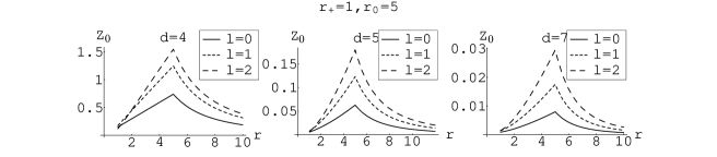
Figure 2: Initial data ${Z_{0}}_{l}$ for a black hole with $r_{+}=1$, and with the particle at $r_{0}=5$, for some values of $l$ the angular quantum number. Again, we show the results for $d=4,\,5$ and $7$ from left to right respectively.

Figure 3: Initial data ${Z_{0}}_{l}$ for a black hole with $r_{+}=1$, and with the particle at $r_{0}=1.5$, for some values of $l$ the angular quantum number. Again, we show the results for $d=4,\,5$ and $7$ from left to right respectively.

In Figs. 2 and 3 we show initial data for an intermediate to large black hole, $r_{+}=1$. In Fig. 2 the fall starts at $r_{0}=5$. We show a typical form of ${Z_{0}}_{l}$ for $r_{+}=1$ and $r_{0}=5$, and for different values of $l$. In Fig. 3 it starts further down at $r_{0}=1.5$. We show a typical form of ${Z_{0}}_{l}$ for $r_{+}=1$ and $r_{0}=1.5$, and for different values of $l$. Again, we have checked that as $r_{0}\rightarrow r_{+}$, all the multipoles fade away, i.e., ${Z_{0}}_{l}\rightarrow 0$, supporting the No Hair Conjecture.

Two important remarks are in order: first, it is apparent from Figs. 1-3 that the field (sum over the multipoles) is divergent at the particle’s position $r_{0}$. This is to be expected, as the particle is assumed to be point-like; second, one is led to believe from Figs. 1-3 (but especially from Figs. 2-3) that ${Z_{0}}_{l}$ increases with $l$. This is not true however, as this behavior is only valid for small values of the angular quantum number $l$. For large $l$, ${Z_{0}}_{l}$ decreases with $l$, in such a manner as to make $\phi(t,r)$ in (3) convergent and finite. For example, for $r_{+}=1,r_{0}=5$ and $d=4$, we have at $r=6$, ${Z_{0}}_{l=20}=0.781$ and ${Z_{0}}_{l=40}=0.3118$.

II.4 Boundary Conditions and the Green’s Function

Equation (7) is to be solved with the boundary conditions appropriate to AdS spacetimes, but special attention must be paid to the initial data lemosvitor : ingoing waves at the horizon,

$${\bf\tilde{Z}}\sim F(\omega)e^{-i\omega r_{*}}+\frac{i{Z_{0}}_{l}}{(2\pi)^{1/2}\omega}\,\,\,,r\rightarrow r_{+}\,,$$ (11)

and since the potential diverges at infinity we impose reflective boundary conditions (${\bf\tilde{Z}}=0$) there avis . Naturally, given these boundary conditions, all the energy eventually sinks into the black hole. To implement a numerical solution, we note that two independent solutions ${\bf\tilde{Z}}^{H}$ and ${\bf\tilde{Z}^{\infty}}$ of (7), with the source term set to zero, have the behavior:

$${\bf\tilde{Z}}^{H}\sim e^{-i\omega r_{*}}\quad\quad r\rightarrow r_{+}\,,$$ (12)

$${\bf\tilde{Z}}^{H}\sim Ar^{d/2-1}+Br^{-d/2}\quad r\rightarrow\infty\,,$$ (13)

$${\bf\tilde{Z}^{\infty}}\sim Ce^{i\omega r_{*}}+De^{-i\omega r_{*}}\quad r\rightarrow r_{+}\,,$$ (14)

$${\bf\tilde{Z}^{\infty}}\sim r^{-d/2}\quad r\rightarrow\infty\,,$$ (15)

(16)

Here, the wronskian $W$ of these two solutions is a constant, $W=2Ci\omega$. Define as in lemosvitor $h^{H}$ through $dh^{H}/dr_{*}=-{\bf\tilde{Z}}^{H}$ and $h^{\infty}$ through $dh^{\infty}/dr_{*}=-{\bf\tilde{Z}^{\infty}}$. We can then show that ${\bf\tilde{Z}}$ given by

$${\bf\tilde{Z}}=\frac{1}{W}\left[{\bf\tilde{Z}^{\infty}}\int_{-\infty}^{r}{\bf\tilde{Z}}^{H}Sdr_{*}+{\bf\tilde{Z}}^{H}\int_{r}^{\infty}{\bf\tilde{Z}^{\infty}}Sdr_{*}\right]+\frac{i\omega}{(2\pi)^{1/2}W}\left[{\bf\tilde{Z}^{\infty}}\int_{-\infty}^{r}h^{H}\frac{d{Z_{0}}_{l}}{dr_{*}}dr_{*}+\right.$$

$${\bf\tilde{Z}}^{H}\int_{r}^{\infty}h^{\infty}\frac{d{Z_{0}}_{l}}{dr_{*}}dr_{*}+\left.(h^{\infty}{Z_{0}}_{l}{\bf\tilde{Z}}^{H}-h^{H}{Z_{0}}_{l}{\bf\tilde{Z}^{\infty}})(r)\right]\,,$$ (17)

is a solution to (7) and satisfies the boundary conditions. In this work, we are interested in computing the wavefunction ${\bf\tilde{Z}}(\omega,r)$ near the horizon ($r\rightarrow r_{+}$). In this limit we have

$${\bf\tilde{Z}}(r\sim r_{+})=\frac{1}{W}\left[{\bf\tilde{Z}}^{H}\int_{r_{+}}^{\infty}{\bf\tilde{Z}^{\infty}}Sdr_{*}\right]+$$

$$\frac{i\omega}{(2\pi)^{1/2}W}{\bf\tilde{Z}}^{H}\left[\int_{r_{+}}^{\infty}{\bf\tilde{Z}^{\infty}}{Z_{0}}_{l}dr_{*}-(h^{\infty}{Z_{0}}_{l})(r_{+})\right]+\frac{i{Z_{0}}_{l}(r_{+})}{(2\pi)^{1/2}\omega}\,,$$ (18)

where an integration by parts has been used.

All we need to do is to find a solution ${\bf\tilde{Z}_{2}}$ of the corresponding homogeneous equation satisfying the above mentioned boundary conditions (16), and then numerically integrate it in (18). In the numerical work, we chose to adopt $r$ as the independent variable, therefore avoiding the numerical inversion of $r_{*}(r)$. To find ${\bf\tilde{Z}_{2}}$,the integration (of the homogeneous form of (7)) was started at a large value of $r=r_{i}$, which was $r_{i}=10^{5}$ typically. Equation (16) was used to infer the boundary conditions ${\bf\tilde{Z}_{2}}(r_{i})$ and ${\bf\tilde{Z}_{2}}^{\prime}(r_{i})$. We then integrated inward from $r=r_{i}$ in to typically $r=r_{+}+10^{-6}r_{+}$. Equation (16) was then used to get $C$.

III Results

III.1 Numerical Results

Our numerical evolution for the field showed that some drastic changes occur when the size of the black hole varies, so we have chosen to divide the results in (i) small black holes and (ii) intermediate and large black holes . We will see that the behavior of these two classes is indeed strikingly different. We refer the reader to lemosvitor for the results in $d=3$.

(i): Wave forms and spectra for small black holes, $r_{+}=0.1$

We plot the waveforms and the spectra. Figs. 4-7 are typical plots for small black holes of waveforms and spectra for $l=0$ and $l=1$ (for $l=2$ and higher the conclusions are not altered). They show the first interesting aspect of our numerical results: for small black holes the $l=0$ signal is clearly dominated by quasinormal, exponentially decaying, ringing modes with a frequency $\omega\sim d-1$ (scalar quasinormal frequencies of Schwarzschild-AdS black holes can be found in HH ; cardosolemos1 ). This particular limit is a pure AdS mode Xpto ; konoplya . For example, Fig. 4 gives, for $d=4$, $\omega=2\pi/T\sim 2\pi/(10/4.5)\sim 2.7$. This yields a value near the pure AdS mode for $d=4$, $\omega=3$. Likewise, Fig. 4 gives $\omega\sim 4$ when $d=5$, the pure AdS mode for $d=5$. All these features can be more clearly seen in the energy spectra plots, Fig. 6, where one can observe the intense peak at $\omega\sim d-1$. The conclusion is straightforward: spacetimes with small black holes behave as if the black hole was not there at all. This can be checked in yet another way by lowering the mass of the black hole. We have done that, and the results we have obtained show that as one lowers the mass of the hole, the ringing frequency goes to $\omega\sim 3$ (for $d=4$) and the imaginary part of the frequency, which gives us the damping scale for the mode, decreases as $r_{+}$ decreases. In this limit, the spacetime effectively behaves as a bounding box in which the modes propagate “freely”, and are not absorbed by the black hole.

Figure 4: The spherically symmetric ($l=0$) waveform for the case of a particle falling from $r_{0}=0.5$ into a $r_{+}=0.1$ black hole. The results are displayed for $d=4,\,5$ and $7$ from left to right respectively. The coordinate $v=t+r_{*}$ is the usual Eddington coordinate.

Figure 5: The $l=1$ waveform for the case of a particle falling from $r_{0}=0.5$ into a $r_{+}=0.1$ black hole.The results are displayed for $d=4,\,5$ and $7$ from left to right respectively.

Figure 6: Typical energy spectra for the spherically symmetric part of the perturbation ($l=0$), here shown for $r_{+}=0.1$, and $r_{0}=0.5$, and for $d=4,\,5$ and $7$. Total energy in this mode: for d=4 we have $E_{l=0,d=4}\sim 75$. For $d=5$, we have $E_{l=0,d=5}\sim 34$. For For $d=7$, we have $E_{l=0,d=7}\sim 1500$.

Figure 7: Typical energy spectra (for $l=1$), here shown for $r_{+}=0.1$, and $r_{0}=0.5$.

Not shown is the spectra for higher values of the angular quantum number $l$. The total energy going down the hole increases slightly with $l$. This would lead us to believe that an infinite amount of energy goes down the hole. However, as first noted in davis2 , this divergence results from treating the incoming object as a point particle. Taking a minimum size $L$ for the particle implies a cutoff in $l$ given by $l_{\rm max}\sim\frac{\pi}{2}\frac{r_{+}}{L}$, and this problem is solved.

(ii): Wave forms and spectra for intermediate and large black holes, $r_{+}=1$

We plot the waveforms and the spectra. As we mentioned, intermediate and large black holes (which are of more direct interest to the AdS/CFT) behave differently. The signal is dominated by a sharp precursor near $v=r_{*0}$ and there is no ringing: the waveform quickly settles down to the final zero value in a pure decaying fashion. The timescale of this exponential decay is, to high accuracy, given the inverse of the imaginary part of the quasinormal frequency for the mode. The total energy is not a monotonic function of $r_{0}$ and still diverges if one naively sums over all the multipoles. In either case, there seem to be no power-law tails, as was expected from the work of Ching et. al. ching . Note that $E$ is given in terms of $E/(q_{s}m_{0}/r)^{2}$. Since $q_{s}m_{0}/r<<1$ the total energy radiated is small in accord with our approximation.

Figure 8: The spherically symmetric ($l=0$) waveform for the case of a particle falling from $r_{0}=5$ into a $r_{+}=1$ black hole. The results are displayed for $d=4,\,5$ and $7$ from left to right respectively.

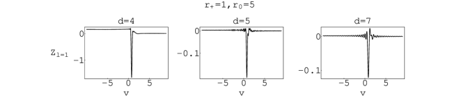
Figure 9: The $l=1$ waveform for the case of a particle falling from $r_{0}=5$ into a $r_{+}=1$ black hole.

Figure 10: Typical energy spectra for the spherically symmetric part of the perturbation ($l=0$), here shown for $r_{+}=1$, and $r_{0}=5$, and for $d=4,\,5$ and $7$.

Figure 11: Typical energy spectra (for $l=1$), here shown for $r_{+}=1$, and $r_{0}=5$.

The value attained by ${\bf\tilde{Z}}$ for large negative $v$ - Fig. 12 - is the initial data, and this can be most easily seen by looking at the value of $Z_{0}$ near the horizon in Fig. 3 (see also lemosvitor ). This happens for small black holes also, which is only natural, since large negative $v$ means very early times, and at early times one can only see the initial data, since no information has arrived to tell that the particle has started to fall. The spectra in general does not peak at the lowest quasinormal frequency (cf Figs. 10, 11 and 13), as it did in flat spacetime davis . (Scalar quasinormal frequencies of Schwarzschild-AdS black holes can be found in HH ; cardosolemos1 ). Most importantly, the location of the peak seems to have a strong dependence on $r_{0}$ (compare Figs. 10 and 13). This discrepancy has its roots in the behavior of the quasinormal frequencies. In fact, whereas in (asymptotically) flat spacetime the real part of the frequency is bounded and seems to go to a constant andersson , in AdS spacetime it grows without bound as a function of the principal quantum number $n$ HH ; cardosolemos1 . Increasing the distance $r_{0}$ at which the particle begins to fall has the effect of increasing this effect, so higher modes seem to be excited at larger distances.

Figure 12: The $l=0$ waveform for the case of a particle falling from $r_{0}=1.5$ into a $r_{+}=1$ black hole.

Figure 13: Typical energy spectra (for $l=0$), here shown for $r_{+}=1$, and $r_{0}=1.5$.

III.2 Discussion of Results

Two important remarks regarding these results can be made:

(i) the total energy radiated depends on the size of the infalling object, and the smaller the object is, the more energy it will radiate. This is a kind of a scalar analog in AdS space of a well known result for gravitational radiation in flat space naka .

(ii) the fact that the radiation emitted in each multipole is high even for high multipoles leads us to another important point, first posed by Horowitz and Hubeny HH . While we are not able to garantee that the damping time scale stays bounded away from infinity (as it seems), it is apparent from the numerical data that the damping time scale increases with increasing $l$. Thus it looks like the late time behavior of these kind of perturbations will be dominated by the largest $l$-mode ($L_{\rm max}\sim\frac{r_{+}}{{\rm size}\,{\rm of}\,{\rm object}}$), and this answers the question posed in HH . Thus a perturbation in $<F^{2}>$ in the CFT ] with given angular dependence $Y_{l}$ on $S^{3}$ will decay exponentially with a time scale given by the imaginary part of the lowest quasinormal mode with that value of $l$.

IV Conclusions

We have computed the scalar energy emitted by a point test particle falling from rest into a Schwarzschild-AdS black hole. ¿From the point of view of the AdS/CFT conjecture, where the (large) black hole corresponds on the CFT side to a thermal state, the infalling scalar particle corresponds to a specific perturbation of this state (an expanding bubble), while the scalar radiation is interpreted as particles decaying into bosons of the associated operator of the gauge theory. Previous works HH ; cardosolemos1 have shown that a general perturbation should have a timescale directly related to the inverse of the imaginary part of the quasinormal frequency, which means that the approach to thermal equilibrium on the CFT should be governed by this timescale. We have shown through a specific important problem that this is in fact correct, but that it is not the whole story, since some important features of the waveforms highly depend on $r_{0}$.

Overall, we expect to find the same type of features, at least qualitatively, in the gravitational or electromagnetic radiation by test particles falling into a Schwarzschild-AdS black hole. For example, if the black hole is small, we expect to find in the gravitational radiation spectra a strong peak located at $\omega^{2}=4n^{2}+l(l+1)\;,\quad n=1,2,...$ cardoso3 . Moreover, some major results in perturbation theory and numerical relativity anninos ; gleiser , studying the collision of two black holes, with masses of the same order of magnitude, allow us to infer that evolving the collision of two black holes in AdS spacetime, should not bring major differences in relation to our results (though it is of course a much more difficult task, even in perturbation theory). In particular, in the small black hole regime, the spectra and waveforms should be dominated by quasinormal ringing.

References

- (1) V. Cardoso, J. P. S. Lemos, Phys. Rev. D 65, 104032 (2002), hep-th/0112254.
- (2) S. Dimopoulos, and G. Landsberg, Phys. Rev. Lett. 87,161602 (2001);
- (3) O. Aharony, S. S. Gubser, J. Maldacena, H. Ooguri, Y. Oz, Phys. Rept. 323, 183 (2000).
- (4) G. T. Horowitz, V. E. Hubeny Phys. Rev. D 62, 024027 (2000).
- (5) V. Cardoso, and J. P. S. Lemos, Phys. Rev. D 64, 084017 (2001).
- (6) V. Cardoso, J. P. S. Lemos, Phys. Rev. D 63, 124015 (2001); S. F. J. Chan and R. B. Mann, Phys. Rev. D 55, 7546 (1997); D. Birmingham, I. Sachs and S. N. Solodukhin, Phys. Rev. Lett. 88, 151301 (2002); J. Zhu, B. Wang, and E. Abdalla, Phys. Rev. D 63, 124004(2001).
- (7) J. M. Maldacena, Adv. Theor. Math. Phys. 2, 253 (1998).
- (8) S. S. Gubser, I. R. Klebanov, A. M. Polyakov, Phys. Lett. B 428, 105 (1998).
- (9) E. Witten, Adv. Theor. Math. Phys. 2, 253 (1998).
- (10) G. ’t Hooft, gr-qc/9310026; L. Susskind, J. Math. Phys. 36, 6377 (1995).
- (11) E. Witten, Adv. Theor. Math. Phys. 2, 505 (1998); T. Banks, M. R. Douglas, G. T. Horowitz, E. Martinec, hep-th/9808016;
- (12) L. Susskind, E. Witten, hep-th/9805114.
- (13) U. H. Danielsson, E. Keski-Vakkuri, M. Kruczenski, Nucl. Phys. B 563, 279 (1999); JHEP 0002, 039 (2000).
- (14) M. Davis, R. Ruffini, W. H. Press, R. H. Price, Phys. Rev. Lett. 27, 1466(1971); for a review see, R. Gleiser, C. Nicasio, R. Price, J. Pullin Phys. Rept. 325, 41 (2000).
- (15) A. Erdelyi, W. Magnus, F. Oberlettinger, and F. Tricomi, Higher Transcendental Functions, (McGraw-Hill Book Co., Inc, New York, 1953); M. Abramowitz, and I. A. Stegun in Handbook of Mathematical Functions, (Dover, New York, 1970); A. F. Nikiforov, V. B. Uvarov, Special Functions of Mathematical Physics, (Birkhäuser, Boston, 1988).
- (16) J. M. Cohen, and R. M. Wald, J. Math. Phys. 12, 1845 (1971).
- (17) L. M. Burko, Class. Quantum Grav. 17, 227 (2000).
- (18) R. Ruffini, in Black Holes: les Astres Occlus, (Gordon and Breach Science Publishers, 1973) R57.
- (19) S. J. Avis, C. J. Isham and D. Storey, Phys. Rev. D 18, 3565 (1978).
- (20) C. Burgess and C. Lutken, Phys. Lett. 153B, 137 (1985).
- (21) R. A. Konoplya, hep-th/0205142.
- (22) M. Davis, R. Ruffini, and J. Tiomno, Phys. Rev. D 5, 2932 (1971).
- (23) E. S. C. Ching, P. T. Leung, W. M. Suen, and K. Young, Phys. Rev. D52, 2118 (1995).
- (24) M. Davis, R. Ruffini, W. H. Press, and R. H. Price, Phys. Rev. Lett. 27, 1466 (1971).
- (25) N. Andersson, Class. Quantum Grav. 10, L61 (1993).
- (26) M. Sasaki and T. Nakamura, Phys. Lett. B 89, 68 (1982).
- (27) P. Anninos, D. Hobill, E. Seidel, L. Smarr, and W. M. Suen, Phys. Rev. Lett. 71, 2851 (1993).
- (28) R. J. Gleiser, C. O. Nicasio, R. H. Price, and J. Pullin, Phys. Rev. Lett. 77, 4483 (1996).