IHES/P/02/35

LPT-Orsay-02/14

OUTP-02/06P

hep-th/0206042

June 2002

EFFECTIVE LAGRANGIANS AND UNIVERSALITY CLASSES OF NONLINEAR BIGRAVITY

Thibault Damour${}^{\,a}$ and Ian I. Kogan${}^{\,a,b,c}$

^a IHES, 35 route de Chartres, 91440, Bures-sur-Yvette, France
^b Laboratoire de Physique Théorique, Université de Paris XI, 91405 Orsay Cédex, France
^c Theoretical Physics, Department of Physics, Oxford University, 1 Keble Road, Oxford, OX1 3NP, UK

Abstract

We discuss the fully non-linear formulation of multigravity. The concept of universality classes of effective Lagrangians describing bigravity, which is the simplest form of multigravity, is introduced. We show that non-linear multigravity theories can naturally arise in several different physical contexts: brane configurations, certain Kaluza-Klein reductions and some non-commutative geometry models. The formal and phenomenological aspects of multigravity (including the problems linked to the linearized theory of massive gravitons) are briefly discussed.

1 Introduction

One of the most important problems which is facing theoretical physics now is the blending of the Standard Model (SM) with General Relativity (GR). Whatever way we choose (the most popular ones nowadays are based on some multidimensional constructions involving extended objects), nobody doubts that it will definitely modify physics at short scales. On the other hand, the current general paradigm is to keep General Relativity unchanged at large scales, but to add new forms of gravitating matter beyond the Standard Model (dark matter, dark energy) for explaining pressing astrophysical and cosmological facts such as galactic rotational curves and the accelerating universe. In the present paper, we consider an alternative paradigm: a modification of General Relativity at large scales as a possible explanation of some pressing cosmological issues (notably cosmic acceleration).

The modification of GR that we are going to consider is linked to the issue of “massive gravity” (for very light gravitons, with Compton wavelength of cosmological scale). A generic prediction of multidimensional constructions is the existence of massive gravitons. In particular, any Kaluza-Klein (KK) model predicts, besides a massless graviton, the presence of an infinite tower of massive gravitons. However, it seems impossible to use the tower of massive KK gravitons to modify gravity at large scales. Indeed, its spectrum is generically regularly spaced (as illustrated on Fig. 1a), so that, even if the first mode were very light (i.e. of cosmological Compton wavelength), there would exist no regime where the first mode (or first few modes) would be important, and where one could truncate away the rest of the tower of massive states. In other words, as soon as the first mode is important, we open the extra KK dimensions (see, however, below). The situation is, however, different in some brane models. In particular, Refs. [1]-[4] discovered the possibility (illustrated in Fig. 1b or Fig. 1c) of having a hierarchical gap, $m_{1}\ll m_{2}$, between the first mode (or first group, or even band, of modes) and the tower of higher modes. This situation, called multigravity (see [5] for a review and [6] for detailed presentation), makes it possible to envisage an effective four-dimensional theory which contains only the massless and ultra-light gravitons and discards the states of mass $m\geq m_{2}$. The constructions [1]-[4] predict see-saw-like spectra, $m_{1}\,M_{\rm Planck}^{1+\gamma}\sim m_{2}^{2+\gamma}$, with $\gamma$ interpolating [5] between $0$ [1] and $1$ [2]. Such spectra are naturally compatible with the phenomenologically interesting situation where $m_{1}^{-1}$ is of cosmological order, while $m_{2}^{-1}$ is smaller than the millimetre scale.

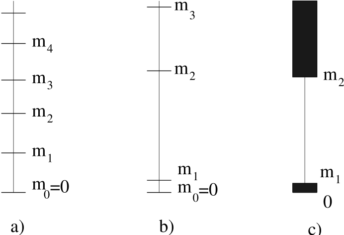
Figure 1: Regular spectrum on (Fig.1 a) versus bigravity (Fig.1 b) or quazi-localized gravity (Fig. 1 c). The last spectrum is continuous but the first band is very narrow in comparison with the gap between bands.

So far multigravity was only analyzed in the linearized approximation. The main emphasis of this paper is to provide a fully non-linear formulation of multigravity, i.e. to write down, and analyze, a class of consistent effective four-dimensional Lagrangians, describing, in some limit, the light-mode truncation of the hierarchical spectra of Figs. 1b or 1c. Though we shall illustrate below our approach in the context of particular multidimensional realizations (notably brane models exhibiting multilocalization [1],[7] or quasi-localization [2], [8], [9]), we view our considerations as concerning a very general phenomenon: the concept of Weakly Coupled Worlds (WCW). The concept of WCW is very simple: one assumes that there are several Universes (labelled by $i=1,\ldots,N$), each endowed with its own metric $g_{(i)\mu\nu}$ and set of matter fields $\{\Phi_{i}\}$, which are coupled only through some mixing of their gravitational fields. We require that the theory describing the WCW be near a point of enhanced symmetry, in the sense that there exists a limit (say as some parameter $\lambda\rightarrow 0$) where the theory contains $N$ diffeomorphism-like symmetries, corresponding to $N$ massless gravitons. A recent theorem [10] has proven that the only consistent non-linear theory involving $N$ massless gravitons is the sum of $N$ decoupled GR-type actions

$$S_{0}=\sum_{i=1}^{N}S[g_{i},\Phi_{i}]\,,$$ (1)

with (we use the signature $-+++$)

$$S[g_{i},\Phi_{i}]=\int d^{4}x\,\sqrt{-g_{i}}\,[M_{i}^{2}R(g_{i})-\Lambda_{i}+L(g_{i},\Phi_{i})]\,.$$ (2)

Therefore, the only consistent action for a theory of worlds coupled only through gravity is of the form

$$S_{\rm tot}=\sum_{i=1}^{N}S[g_{i},\Phi_{i}]+\lambda\,S_{\rm int}(g_{1},g_{2},\ldots,g_{N})\,.$$ (3)

When $\lambda\rightarrow 0$, the $N$ worlds are non interacting (which implies that, from the point of view of any observer in one world, the other worlds have only a meta-physical existence), and the theory has the enormous symmetry $\Pi_{i}{\rm Diff}_{(i)}$, where each diffeomorphism group ${\rm Diff}_{(i)}$ acts separately on its own metric $g_{(i)\mu\nu}$ and matter fields $\{\Phi_{i}\}$. In the interacting case, $\lambda\neq 0$, the symmetry of the full action must (again because of the theorem [10]) be reduced to (at most) one group of diffeomorphisms: the diagonal group of common diffeomorphisms transforming all metrics as

$$\delta\,g_{\mu\nu}^{(i)}=\epsilon^{\lambda}\,\partial_{\lambda}\,g_{\mu\nu}^{(i)}+\partial_{\mu}\,\epsilon^{\lambda}\,g_{\lambda\nu}^{(i)}+\partial_{\nu}\,\epsilon^{\lambda}\,g_{\mu\lambda}^{(i)}\equiv D_{\mu}^{(i)}\,\epsilon_{\nu}+D_{\nu}^{(i)}\,\epsilon_{\mu}\,.$$ (4)

This symmetry restricts the interaction term $\lambda\,S_{\rm int}(g_{1},\ldots,g_{N})$ to depend only on the invariants one can make with several metrics. This even leaves room for extra kinetic terms built from covariant derivatives such as $g_{(i)}^{\mu\nu}\,D_{\lambda}^{(j)}\,g_{\mu\nu}^{(k)}$ (such terms do not exist in the case of one metric because $D_{\lambda}^{(i)}\,g_{\mu\nu}^{(i)}\equiv 0$). However, in view of the many potential diseases associated to modifications of the standard Einsteinian kinetic terms, and in the spirit of describing the class of interaction terms most relevant at large scales, i.e. containing the lowest possible number of derivatives ( namely zero, as expected from a generalization of the mass terms that appear in linearized multigravity), we shall only consider ultra-local interaction terms, i.e.

$$\lambda\,S_{\rm int}=-\mu^{4}\int d^{4}x\,{\cal V}(g_{1}(x),\ldots,g_{N}(x))\,,$$ (5)

where $\mu$ is a mass scale (henceforth replacing $\lambda$ as “small parameter”) and where ${\cal V}$ is a scalar density made out of the values of the $N$ metrics at the same “point”. We assume, for simplicity, that the $N$ weakly coupled worlds “live” on the same abstract manifold, i.e., in other terms, that one is given a family of (smooth) canonical one-to-one maps: ${\rm world}_{(i)}\rightarrow{\rm world}_{(j)}$.

The aim of this paper is threefold: (i) to motivate the possibility of the effective action (3), (5) by considering several different specific models (brane models, Kaluza-Klein models and non-commutative geometry ideas); (ii) to delineate and parametrize the various “universality classes” of non-linear multigravity; and (iii) to sketch the main qualitative consequences of such non-linear multigravity theories and to contrast them with the usual paradigm of “massless plus massive gravitons” which is based on a linearized approximation.

It should be noted that theories defined by (3), (5) (in the “bigravity” case: $N=2$) were first introduced in the seventies [11] as a model for describing a sector of hadronic physics where a massive spin-2 field (the “$f$ meson”, with “Planck mass” $M_{f}\sim 1\,{\rm GeV}$ in Eq. (2)) plays a dominant role. It was then called “strong gravity” or the “$f$-$g$ theory”. Our work not only proposes to revive, within a new (purely “gravitational”) physical context, this early proposal, but initiates the task of systematically studying the general phenomenological consequences of the action (3), (5). The present paper will only briefly sketch the new physical paradigm following from such actions. In subsequent papers, we shall discuss in detail the cosmological consequences of such theories [12], as well as its strong-field phenomenology [13].

2 Universality Classes of Bigravity Effective
Lagrangians

For simplicity, we focus, in this paper, on the case of “bigravity”, i.e. $N=2$. Understanding this case is a prerequisite for understanding the general multigravity case ($N>2$). Let us note also that the bigravity “potentials” that we discuss here can be immediately used in the general case. Indeed a rather general class of “$N$-metric potentials” ${\cal V}(g_{(1)},\ldots,g_{(N)})$, Eq. (5), is the class containing only “two-metric interactions”: ${\cal V}=\sum_{i\neq j}{\cal V}(g_{(i)},g_{(j)})$. For instance, one can define a “crystal-like” many-world with “nearest neighbour” interactions only ${\cal V}=\sum_{i}{\cal V}(g_{(i)},g_{(i+1)})$. It is interesting to note that the continuum limit ($N\rightarrow\infty$) for some suitable “nearest neighbour” interactions can mimic the propogation of gravity in a higher-dimensional space, i.e. the term $\int dya^{4}(y)\,\sqrt{-g(x,y)}\left[{\rm tr}(g^{-1}\,\partial_{y}\,g)^{2}-({\rm tr}\,g^{-1}\,\partial_{y}\,g)^{2}\right]\,.$ as in (29) below. See [12] for further discussion of this subject.

2.1 Parametrization of invariants

Using, when $N=2$, the notation $g_{(1)}=g_{L}$ (for “Left”) and $g_{(2)}=g_{R}$ (for “Right”), and factoring a conventional “average volume factor” $(g_{L}\,g_{R})^{1/4}$ out of the scalar density ${\cal V}$ , the generic bigravity action reads

$$S=\int d^{4}x\,\sqrt{-g_{L}}\left(M_{L}^{2}\,R(g_{L})-\Lambda_{L}\right)+\int d^{4}x\,\sqrt{-g_{L}}\,L(\Phi_{L},g_{L})+$$

$$\int d^{4}x\,\sqrt{-g_{R}}\left(M_{R}^{2}\,R(g_{R})-\Lambda_{R}\right)+\int d^{4}x\,\sqrt{-g_{R}}\,L(\Phi_{R},g_{R})$$

$$-\mu^{4}\int d^{4}x\left(g_{R}\,g_{L}\right)^{1/4}V(g_{L},g_{R})\,.$$ (6)

Note that the bigravity action (6) contains 5 dimensionfull parameters: two “Planck masses” $M_{L}$ and $M_{R}$, two cosmological constants $\Lambda_{L}$, $\Lambda_{R}$ (with dimensions $M^{4}$), and the “coupling mass scale” $\mu$.

Before proceeding, we note that the mass scale $\mu$, entering Eq. (6), will be treated here as a constant parameter determining the coupling of the two worlds. However, one should keep in mind the possibility that it be replaced by a fluctuating field. This is suggested, in particular, by the brane realizations of bigravity where the value of $\mu$ depends on the physical distance between the branes, which is controlled by dilaton/radion fields. A more general model where $\mu\rightarrow\mu(x)$, and where one adds a kinetic term for $\mu(x)$, may play an important role in addressing crucial cosmological issues (such as inflation) in the context of multigravity theories.

Before we shall proceed further let us make two additional comments

• We shall treat $V$ as a potential here, i.e. as an ultra-local function of $g_{L}$ and $g_{R}$. As already mentioned above one could also include extra kinetic terms like $g^{\mu\nu}D^{L,R}_{\mu}g_{R,L}^{\sigma\rho}D^{L,R}_{\nu}g_{L,R~{}\sigma\rho}$, etc. For example mixed terms like $\sqrt{-g_{L}}R(g_{R})$ or $\sqrt{-g_{R}}R(g_{L})$ are of these type. However, let us emphasise again that the fundamental concept of WCW explored here is that one is required to be near the point of enhanced symmetry and according to the theorem proven in [10] in this point mixing of different metrics is forbidden. Because of this all higher derivative terms mixing different metrics must be supressed by the small parameter $\mu^{4}$ and enter as $\mu^{4}f(D^{2}g/M^{2})$. One can see that in the long-wave limit $D^{2}g/M^{2}\sim k^{2}/M^{2}<<1$ one can neglect their contribution in comparison with a potential term.

• Let us stress that we did not introduce any direct coupling between the two worlds exept the indirect one mediated by gravity. It means that all matter which can be observed by any observer is locally coupled only to one world or the other one. Thus any local experimental check of the equivalence principle is the same as in the General Relativity - all locally mutually observable matter moves in the same metric. One can consider other cases but such a study will be left for future publications.

The common diffeomorphism invariance (4) restricts the scalar potential $V(g_{L},g_{R})$ entering Eq. (6) to depend only on the invariants of the mixed tensor $H\equiv g_{L}^{-1}\,g_{R}$, i.e.

$$H_{\nu}^{\mu}\equiv g_{L}^{\mu\sigma}\,g_{R\sigma\nu}\,.$$ (7)

In 4 dimensions, there are (because of Cayley’s theorem) only 4 independent scalar invariants which can be made from $H$. For instance, using a matrix notation for $H$, one can take the first 4 traces of the powers of the matrix $H$, say

$$\tau_{n}\equiv{\rm tr}(H^{n})\,;\qquad n=1,2,3,4\,.$$ (8)

Let us introduce the 4 eigenvalues $\lambda_{a}$ ($a=0,\ldots,3$) of $H_{\nu}^{\mu}$, i.e. the 4 eigenvalues of the metric $g_{R}$ with respect to $g_{L}$. They can be defined either by $\tau_{n}=\Sigma_{a}\,\lambda_{a}^{n}$, or by writing the two metrics in a special bi-orthogonal vierbein $e_{\mu}^{a}$ such that

$$g_{\mu\nu}^{L}=-e_{\mu}^{0}\,e_{\nu}^{0}+e_{\mu}^{1}\,e_{\nu}^{1}+e_{\mu}^{2}\,e_{\nu}^{2}+e_{\mu}^{3}\,e_{\nu}^{3}\,,$$

$$g_{\mu\nu}^{R}=-\lambda_{0}\,e_{\mu}^{0}\,e_{\nu}^{0}+\lambda_{1}\,e_{\mu}^{1}\,e_{\nu}^{1}+\lambda_{2}\,e_{\mu}^{2}\,e_{\nu}^{2}+\lambda_{3}\,e_{\mu}^{3}\,e_{\nu}^{3}\,.$$ (9)

It is easily seen that, apart from an exceptional case (where two eigenvalues coincide, and correspond to a null eigenvector), it is generically possible to write Eq. (9), though maybe with a complex vierbein $e_{\mu}^{a}$. Indeed, two (but at most two) eigenvalues, say $\lambda_{0}$, $\lambda_{1}$ (one of which necessarily corresponds to a time-like direction) can become complex. We shall focus on the case where the 4 eigenvalues $\lambda_{0}$, $\lambda_{1}$, $\lambda_{2}$, $\lambda_{3}$ are real and positive. As we shall only deal with symmetric functions of the eigenvalues, this restriction is mainly a notational convenience which can be relaxed by analytic continuation. It is then convenient to parametrize the invariants of $H=g_{L}^{-1}\,g_{R}$ by means of the logarithms of the eigenvalues of $H$:

$$\mu_{a}\equiv\ln\,\lambda_{a}\ ;\quad\lambda_{a}\equiv e^{\mu_{a}}\,,$$ (10)

(the $\mu_{a}$’s should not be confused with the mass scale $\mu^{4}$ in front of $V$) and to introduce, as basis of independent scalars, the 4 symmetric polynomials

$$\sigma_{n}\equiv\sum_{a}\mu_{a}^{n}\,.$$ (11)

With this notation, our first result is that the most general (densitized) potential can be written as

$$\mu^{4}\,{\cal V}(g_{L},g_{R})=\mu^{4}(g_{L}\,g_{R})^{\frac{1}{4}}\,V(\sigma_{1},\sigma_{2},\sigma_{3},\sigma_{4})\,,$$ (12)

where $V$ is an arbitrary function of the 4 $\sigma_{a}$’s.

2.2 Universality classes

In the same way as the various mathematical forms of the Landau free energy define universality classes of phase transitions, we can define universality classes of bigravity theories by considering as equivalent the functions $V(\sigma_{a})$ leading to (essentially) the same multi-gravitational phenomenology. As we shall see below and in [12, 13], some of the important qualitative features of the function $V(\sigma_{a})$ are: (i) its behaviour near $\sigma_{a}\rightarrow 0$, (ii) its behaviour when $\sigma_{a}\rightarrow\infty$, and (iii) the existence or non-existence of “critical points” where some derivatives $\partial V/\partial\sigma_{a}$ vanish.

As a first example of a universality class, we can define the class of $V$’s which reduce (in absence of cosmological constants in (6), i.e. $\Lambda_{L}=\Lambda_{R}=0$), in the linearized approximation, to the Pauli-Fierz mass term $\sim h_{\nu}^{\mu}\,h_{\mu}^{\nu}-h_{\mu}^{\mu}\,h_{\nu}^{\nu}$. The linearized approximation corresponds to the particular case where $g_{L\mu\nu}$ and $g_{R\mu\nu}$ are both near the same flat metric $\eta_{\mu\nu}$, i.e. $g_{L\mu\nu}=\eta_{\mu\nu}+h_{\mu\nu}^{L}$, $g_{R\mu\nu}=\eta_{\mu\nu}+h_{\mu\nu}^{R}$, with $h_{L}\ll 1$ and $h_{R}\ll 1$. In this limit the above object $H=g_{L}^{-1}\,g_{R}$ reads $H_{\nu}^{\mu}\simeq\delta_{\nu}^{\mu}+h_{R\nu}^{\mu}-h_{L\nu}^{\mu}$ (where the indices on $h_{R}$ and $h_{L}$ are raised by $\eta^{\mu\nu}$). It is then seen that the eigenvalues of $H$ are $\lambda_{a}\simeq 1+\mu_{a}$, where $\mu_{a}\ll 1$ are the eigenvalues of $h_{R\nu}^{\mu}-h_{L\nu}^{\mu}$. With the identification of the massive graviton mode $h_{\mu\nu}$ as $h_{\mu\nu}=h_{\mu\nu}^{R}-h_{\mu\nu}^{L}$ (see below), one then sees that the Pauli-Fierz mass term $\sim h_{\nu}^{\mu}\,h_{\mu}^{\nu}-h_{\mu}^{\mu}\,h_{\nu}^{\nu}$ is obtained if the function $V(\sigma_{a})$ behaves (modulo a positive factor that can be absorbed in the mass scale $\mu^{4}$) as

$$V(\sigma_{a})\simeq\sigma_{2}-\sigma_{1}^{2}=\sum_{a}\mu_{a}^{2}-\left(\sum_{a}\mu_{a}\right)^{2}\,,\quad\hbox{when}\ \mu_{a}\rightarrow 0\,.$$ (13)

The behaviour (13) near $\mu_{a}\rightarrow 0$ defines the universality class of “Pauli-Fierz-like” bigravity. Note that one can imagine a case where the potential $V$ does not have quadratic terms when $\mu_{a}\rightarrow 0$. In the linearized approximation, one would see two massless gravitons, while the full theory would contain two interacting metric field $g_{L},g_{R}$ (and only one common diffeomorphism invariance).

As a second example of the concept of universality class, we can define the class of potentials ${\cal V}(g_{L},g_{R})$ which are symmetric under the exchange $g_{L}\leftrightarrow g_{R}$. It is easily seen that under the exchange $L\leftrightarrow R$, the eigenvalues $\lambda_{a}$ get inverted $(\lambda_{a}\rightarrow\lambda_{a}^{-1})$ so that the logarithmic eigenvalues $\mu_{a}$ change sign: $\mu_{a}\rightarrow-\mu_{a}$. The class of exchange-symmetric potentials therefore corresponds to the class of functions $V(\mu_{a})$ which are even in the $\mu_{a}$’s. In terms of the $\sigma$’s this becomes $V(\sigma_{1},\sigma_{2},\sigma_{3},\sigma_{4})=V(-\sigma_{1},\sigma_{2},-\sigma_{3},\sigma_{4})$.

As a further example of universality class, we can consider the class of functions which depend only on the first two invariants $\sigma_{1}\equiv\sum_{a}\mu_{a}$ and $\sigma_{2}=\sum_{a}\mu_{a}^{2}:V=V(\sigma_{1},\sigma_{2})$. We shall see that this class appears naturally in brane models, and our (preliminary) investigations suggest that this class might be general enough to describe all the possible qualitative features of a general bigravity theory.

2.3 Equations of motion

The equations of motion derived from the bigravity action read

$$2\,M_{L}^{2}\left(R_{\mu\nu}(g^{L})-\frac{1}{2}\,g_{\mu\nu}^{L}\,R(g^{L})\right)+\Lambda_{L}\,g_{\mu\nu}^{L}=t_{\mu\nu}^{L}+T_{\mu\nu}^{L}\,,$$

$$2\,M_{R}^{2}\left(R_{\mu\nu}(g^{R})-\frac{1}{2}\,g_{\mu\nu}^{R}\,R(g^{R})\right)+\Lambda_{R}\,g_{\mu\nu}^{R}=t_{\mu\nu}^{R}+T_{\mu\nu}^{R}\,.$$ (14)

Here $T_{L}^{\mu\nu}\equiv 2(-g_{L})^{-1/2}\,\delta\,S_{\rm matter}^{L}/\delta\,g_{\mu\nu}^{L}$ denotes the stress-energy tensor of the matter on the left brane $(S_{\rm matter}^{L}=\int d^{4}x\,\sqrt{-g_{L}}\,L(\Phi_{L},g_{L}))$, while $t_{L}^{\mu\nu}\equiv g_{L}^{\mu\alpha}\,g_{L}^{\nu\beta}\,t_{\alpha\beta}^{L}$ denotes the effective stress-energy tensor (as seen on the left brane) associated to the coupling term $S_{\rm int}\equiv-\mu^{4}\int d^{4}x(g_{R}\,g_{L})^{1/4}\,V(g_{L},g_{R})$:

$$t_{L}^{\mu\nu}\equiv\frac{2}{\sqrt{-g_{L}}}\,\frac{\delta\,S_{\rm int}(g_{L},g_{R})}{\delta\,g_{\mu\nu}^{L}}=-2\,\mu^{4}\left(\frac{g_{R}}{g_{L}}\right)^{\frac{1}{4}}\left[g^{\mu\nu}_{L}\,\frac{V}{4}+\frac{\partial\,V(g_{L},g_{R})}{\partial\,g_{\mu\nu}^{L}}\right]\,.$$ (15)

The corresponding expressions for the right brane are obtained by the exchange $L\leftrightarrow R$. For instance

$$t_{R}^{\mu\nu}=-2\,\mu^{4}\left(\frac{g_{L}}{g_{R}}\right)^{\frac{1}{4}}\left[g^{\mu\nu}_{R}\,\frac{V}{4}+\frac{\partial\,V(g_{L},g_{R})}{\partial\,g_{\mu\nu}^{R}}\right]\,.$$ (16)

The Bianchi identities $\left(D_{L}^{\nu}\left(R_{\mu\nu}^{L}-\frac{1}{2}\,R^{L}\,g_{\mu\nu}^{L}\right)\equiv 0\right)$, and the conservation of the material energy tensor ($D_{L}^{\nu}\,T_{\mu\nu}^{L}=0;$ when the matter equations of motion are satisfied) imply the constraints:

$$D_{L}^{\nu}\,t_{\mu\nu}^{L}=0\quad\hbox{and}\quad D_{R}^{\nu}\,t_{\mu\nu}^{R}=0\,.$$ (17)

Actually these two constraints are not independent because the invariance of $S_{\rm int}$ under the unbroken diagonal diffeomorphism group implies the identity

$$\sqrt{-g_{L}}D_{L}^{\nu}\,t_{\mu\nu}^{L}+\sqrt{-g_{R}}D_{R}^{\nu}\,t_{\mu\nu}^{R}\equiv 0\,.$$

The explicit expressions of the derivative terms $\partial\,V/\partial\,g_{\mu\nu}^{L,R}$ in Eqs. (15), (16) tends to be rather complicated. However, they acquire a simple form when written in the special frames with respect to which both $g_{\mu\nu}^{L}$ and $g_{\mu\nu}^{R}$ are diagonalized (such as in Eq. (9)). The mixed components of $t_{\mu\nu}^{L}$ and $t_{\mu\nu}^{R}$ with respect to any such frame (which can differ from the particular $e_{\mu}^{a}$ of (9) by arbitrary rescalings $e_{\mu}^{a}\rightarrow\zeta^{a}\,e_{\mu}^{a}$, because such rescalings leave $t_{La}^{a}$ and $t_{Ra}^{a}$ invariants) take the simple form: (no summation on the frame index $a$)

$$t_{La}^{a}=-2\,\mu^{4}\,e^{\frac{1}{4}\sigma_{1}}\left(\frac{V}{4}-\frac{\partial\,V}{\partial\,\mu_{a}}\right)\,,$$

$$t_{Ra}^{a}=-2\,\mu^{4}\,e^{-\frac{1}{4}\sigma_{1}}\left(\frac{V}{4}+\frac{\partial\,V}{\partial\,\mu_{a}}\right)\,,$$ (18)

with vanishing of the off-diagonal components (we recall: $\sigma_{1}\equiv\sum_{b}\mu_{b}$).

Here, we considered the scalar potential as a function of the $\mu_{a}$’s. If $V$ is given as a function of the $\sigma_{n}$’s, Eq. (11), the derivative entering Eqs. (18) takes the explicit:

$$\frac{\partial\,V(\sigma_{1},\ldots,\sigma_{4})}{\partial\,\mu_{a}}=\frac{\partial\,V}{\partial\,\sigma_{1}}+2\,\mu_{a}\,\frac{\partial\,V}{\partial\,\sigma_{2}}+3\,\mu_{a}^{2}\,\frac{\partial\,V}{\partial\,\sigma_{3}}+4\,\mu_{a}^{3}\,\frac{\partial\,V}{\partial\,\sigma_{4}}\,.$$ (19)

This explicit expression illustrates the third type ((iii)) of universality class mentioned above: If there exist “critical points” where $\partial_{\sigma_{2}}\,V=\partial_{\sigma_{3}}\,V=\partial_{\sigma_{4}}\,V=0$ (without restriction on $\partial_{\sigma_{1}}\,V$), such points give rise to a $t_{L\nu}^{\mu}$ and a $t_{R\nu}^{\mu}$ with the local “equation of state” $t_{L0}^{0}=t_{L1}^{1}=t_{L2}^{2}=t_{L3}^{3}$ (and similarly for $t_{R}$), i.e. such that $t_{\mu\nu}^{L}\propto g_{\mu\nu}^{L}$ and $t_{\mu\nu}^{R}\propto g_{\mu\nu}^{R}$. In some cases, such critical points can be “fixed points” and can give rise (in the “vacuum case”, i.e. in absence of “material” $T_{\mu\nu}^{L,R}$) to bi-(A)dS solutions of the coupled field equations. Note in this respect that the “perturbative limit” $\mu_{a}=0$ is a critical point in the sense that $\partial_{\mu_{a}}\,V=\partial_{\sigma_{1}}\,V$, independently of the value of $a$, so that $\mu_{a}=0$ (i.e. $g_{\mu\nu}^{L}=g_{\mu\nu}^{R}$) can be a (perturbative) fixed point of the coupled vacuum equations, corresponding to a bi-(A)dS solution, if the corresponding (constant) curvature $\lambda$ ($R_{L\nu}^{\mu}=\lambda\,\delta_{\nu}^{\mu}=R_{R\nu}^{\mu}$) satisfies the two equations

$$-2\,\lambda\,M_{L}^{2}+\Lambda_{L}=-2\,\mu^{4}\left[\frac{V}{4}-\partial_{\sigma_{1}}\,V\right]_{\mu_{a}=0}\,,$$

$$-2\,\lambda\,M_{R}^{2}+\Lambda_{R}=-2\,\mu^{4}\left[\frac{V}{4}+\partial_{\sigma_{1}}\,V\right]_{\mu_{a}=0}\,.$$ (20)

In the “Pauli-Fierz” universality class the right-hand sides of Eqs. (20) vanish and one has the usual relation $\lambda=\Lambda_{L}/(2\,M_{L}^{2})$ (with the constraint $\Lambda_{L}/M_{L}^{2}=\Lambda_{R}/M_{R}^{2}$). In more general classes the coupling between the two worlds can modify the usual link between $\lambda$ and $\Lambda_{L,R}$.

2.4 Single “massive graviton” as a limiting case of bigravity

Let us consider the formal limit $M_{R}\rightarrow\infty$ in the action (6) (and the field equations (14)). In this limit the metric $g_{R}$ is (formally) frozen into some given “background” metric $G_{\mu\nu}:g_{R}\rightarrow G$, with $G_{\mu\nu}$ solution of $R_{\mu\nu}(G)=\lambda\,G_{\mu\nu}$, where $\lambda=\lim(\Lambda_{R}/(2\,M_{R}^{2}))$ can be zero, or can be arranged to take any fixed real value. This leaves us with an action for a single dynamical metric $g\equiv g_{L}$ of the form

$$S=\int d^{4}x\sqrt{-g}\,(M_{L}^{2}\,R(g)-\Lambda_{L})-\mu^{4}\int d^{4}x\,(g\,G)^{\frac{1}{4}}\,V(G^{-1}\,g)\,.$$ (21)

If $V$ belongs to the Pauli-Fierz universality class, $g_{\mu\nu}=G_{\mu\nu}$ is a solution of the equations of motion (if $\lambda=\Lambda_{L}/(2\,M_{L}^{2}))$, and the small excitations of $g_{\mu\nu}$ around $G_{\mu\nu}$ describe a “massive graviton” (propagating in an Einstein space). But the behaviour of the large excitations of $g_{\mu\nu}$ are described by the non-linear action (21) instead of the usual quadratic Pauli-Fierz action.

The action (21) is (formally) generally covariant: when $g$ is transformed as (4), the frozen metric $G$ must also be transformed as $\delta\,G_{\mu\nu}=D_{\mu}^{G}\,\epsilon_{\nu}+D_{\nu}^{G}\,\epsilon_{\mu}$. These fluctuations of $G$ (which do not change the background curvature invariants) are playing the same role as the Goldstone degrees of freedom in the Higgs mechanism for gauge fields. In a recent paper [14] these Goldstone degrees of freedom were discussed for the single AdS₄ brane case, using an holographic description of five-dimensional gravity in terms of a four-dimensional CFT, and it was shown that there is indeed a vector field which provides extra components to the graviton.

3 Specific Examples of Bigravity Effective
Lagrangians

After having discussed general possible structural features of bigravity effective Lagrangians, we shall consider specific physical models in which such Lagrangians arise. We consider in turn: (i) brane models, (ii) Kaluza-Klein models, and (iii) non-commutative-type models. Beforehand let us note that the work in the seventies that first considered bigravity models did not have any underlying physical models from which they could derive some specific potentials $V(g_{L},g_{R})$. They made up some non-linear generalizations of the quadratic Pauli-Fierz mass term. For instance, they particularly considered the one-parameter family of models with

$$V(g_{L},g_{R})\propto\left(\frac{g_{R}}{g_{L}}\right)^{a}(g_{\alpha\mu}^{L}\,g_{\beta\nu}^{L}-g_{\alpha\beta}^{L}\,g_{\mu\nu}^{L})(g_{R}^{\alpha\beta}-g_{L}^{\alpha\beta})(g_{R}^{\mu\nu}-g_{L}^{\mu\nu})\,.$$ (22)

3.1 Brane models

Let us start by briefly recalling why (multi-)brane models naturally give rise to “multigravity”. For more details the reader is advised to look at the original papers, and/or at reviews such as, [15], [5]. Before explaining how several worlds can be gravitationally “weakly coupled”, let us recall that the paradigmatic brane example of a separate (gravitationally decoupled) brane world is a Randall-Sundrum (RS) scenario, i.e. a flat 3-brane in AdS(5), with jump conditions on the brane (coming from an assumed $Z_{2}$ symmetry) able to “localize” the 5-dimensional graviton as a massless excitation propagating (as a “surface wave”) in the vicinity of the brane [16], [17]. Putting the brane at the point $y=0$ (where $y$ is the “fifth”, transversal coordinate, and where one requires the $Z_{2}$ symmetry $y\rightarrow-y$), the background 5-dimensional geometry is (see Fig. 2a)

$$ds^{2}=e^{-2\sigma(y)}\eta_{\mu\nu}dx^{\mu}dx^{\nu}+dy^{2}=e^{-2\sigma(z)}\left[\eta_{\mu\nu}dx^{\mu}dx^{\nu}+dz^{2}\right]\,.$$ (23)

The warp factor behaves as $\sigma(y)\sim|y|\sim\ln(1+|z|)$. The fluctuations near the background metric are studied by writing:

$$ds^{2}=e^{-2\sigma(z)}\left[\left(\eta_{\mu\nu}+h_{\mu\nu}(x,z)\right)dx^{\mu}dx^{\nu}+dz^{2}\right]\,.$$ (24)

The field $h_{\mu\nu}(x,z)$ is expanded in terms of the graviton and KK plane wave states : $h_{\mu\nu}(x,z)=\sum_{n=0}^{\infty}\exp\left(\frac{3}{2}\,\sigma\right)h_{\mu\nu}^{(n)}(x)\Psi_{n}(z)$ where the $\exp\left(\frac{3}{2}\,\sigma\right)$ factor in the expansion is necessary for the functions $\Psi^{(n)}(z)$ to obey an ordinary Schrödinger equation:

$$\left\{-\partial_{z}^{2}+V(z)\right\}\Psi_{n}(z)=m_{n}^{2}\Psi_{n}(y)\,.$$ (25)

Here the potential $V(z)=(dA/dz)^{2}-d^{2}A/dz^{2}$ where $A=3\sigma(z)/2$. Qualitatively it is made up of an attractive $\delta$-function potential plus a smoothing term (due to the AdS geometry) that gives the attractive potentials a “volcano” form. An interesting characteristic of this potential is that it gives rise to a (massless) normalizable zero mode

$$\Psi_{0}(z)=\exp[-A(z)]=\exp[-\frac{3}{2}\,\sigma(z)]$$ (26)

One can show (see for details [18] and references therein) that the normalization factor $\int dz\Psi_{0}^{2}=\int dz\exp[-3\sigma(z)]$ also relates the fundamental five-dimensional mass scale $M_{5}$ to the four-dimensional Planck mass $M_{p}$, namely $M_{p}^{2}=M_{5}^{3}\int dz\exp[-3\sigma(z)]$.

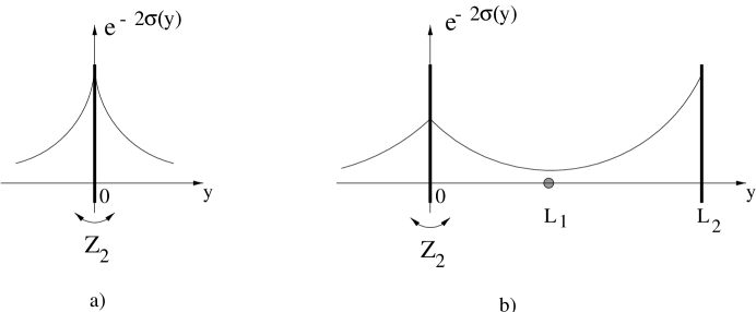
Figure 2: Warped metric for single flat brane (Fig. 2a) and bounce for a two-brane configuration (Fig. 2b). $L_{2}$ is the separation between branes and $L_{1}$ is the position of the bounce. If $L_{1}\ll L_{2}$ the metric is mostly concentrated on a right brane and if $L_{2}-L_{1}\ll L_{1}$ then it is concentrated on the left brane.

One can consider now multibrane configurations where the warped metric is a bounce as on Fig. 2b. By analysing the spectrum in this case one can easily see that in the case of an infinitely large separation between the branes massless gravitons are localized on both of them. But then, according to basic properties of the Shrödinger equation, when the separation is finite, the degeneracy between the two massless modes is removed and one ends up with one massless and one ultralight massive graviton. The prototype model of this class was the “$+-+$ bigravity” model [1] with two positive tension flat branes (${}^{\prime\prime}+^{\prime\prime}$ branes) separated at the bounce position $L_{1}$ by one intermediate negative tension flat brane (${}^{\prime\prime}-^{\prime\prime}$ brane) in an $AdS_{5}$ bulk. The task of finding the KK spectrum reduces to a simple quantum mechanical problem. It is simple to see that the model (as every compact model) has a massless graviton that corresponds to the ground state of the system whose wave function follows the “warp” factor. Then it is easy to see that (say, for simplicity, in the symmetric case $L_{2}=2L_{1}$) there should be a state with wave function antisymmetric with respect to the minimum of the “warp” factor, whose mass splitting from the massless graviton will be very small compared to the masses of the higher levels. Because the “warp” factor is exponential the difference in mass behaviour of the first and the rest of the KK states is also exponential. This allowed for the construction of a linear “bigravity” model in which the remainder of the KK tower does not affect gravity beyond the millimetre bound. Soon after this model, other models were discussed. Some of them, for example the “quasi-localized” GRS model [2] and a more general $+--+$ multigravity model [3], [4] also used dynamical negative tension branes. In other models, like the $++$ model with two $AdS_{4}$ branes [19] (or the limiting case of one single $AdS_{4}$ brane when the second one is moved to infinity [20]) or in a six-dimensional case [21], there are no negative tension branes and so no problems emerge with ghost-like radion states. Models with moving branes in which one also can get “warped” factors were discussed in [22]-[23]. Finally there is a whole zoo of different models in which one can get modification of gravity at large scales.

To be specific, let us consider the $+-+$ model and let us now derive the fully non-linear bigravity action it gives rise to in the weak-coupling limit where we keep only the dominant terms in the exponentially small (“tunnelling”) coupling between the two positive tension branes. We are going to ignore the fact that there is a ghost-like radion field due to the existence of the negative tension brane in this model [24]. Anyway we freeze all dilaton and radion degrees of freedom.

The action describing the full 5-dimensional configuration is (in units where the five-dimensional Planck mass is set to one)

$$S=\int d^{4}x\int dy\,\sqrt{-G}\left[R(G)-V_{b}-\sum_{i}V_{i}\,\delta(y-y_{i})\right]\,.$$ (27)

Here, $G$ denotes the 5-dimensional metric, $V_{b}$ the bulk cosmological constant, and $V_{i}$ the tensions of the branes (the index $i$ takes, in our case, three values corresponding to the three branes: e.g. $V_{1}=V_{L}>0$, $V_{2}<0$ and $V_{3}=V_{R}>0$). We generalize the linear fluctuation ansatz (24) by writing the 5-dimensional metric as ($\mu,\nu=0,1,2,3$)

$$ds_{5}^{2}=a^{2}(y)\,g_{\mu\nu}(x,y)\,dx^{\mu}\,dx^{\nu}+dy^{2}\,,$$ (28)

where $a^{2}(y)=e^{-2\sigma(y)}$ is the background warp factor. We assume here that the degrees of freedom associated to the fluctuations of: (i) the warp factor (“dilaton”), and (ii) the distance between the branes (“radions”) are all frozen. The detailed mechanism of how to do that is not important for us now. For example, one can add extra terms in the action (27) that give large enough mass terms to these fluctuations (say with submillimeter Compton wave length) following [25] (of course for those radion fields which are ghost-like one has to add tachyonic mass terms). The fluctuations of the mixed components $g_{\mu y}$ can be consistently set to zero, because of the $Z_{2}$ symmetry requirement. Inserting the ansatz (28) into the action (27) yields, after integration by parts and use of the background equations of motion for the warp factor (which allow one to dispose of all terms containing $y$-gradients of $a(y)$) the following action for $g_{\mu\nu}(x,y)$

$$S=\int d^{4}x\int dy\,\sqrt{-g(x,y)}\left\{a^{2}(y)\,R(g(x,y))-\frac{1}{4}\,a^{4}(y)\left[{\rm tr}(g^{-1}\,\partial_{y}\,g)^{2}-({\rm tr}\,g^{-1}\,\partial_{y}\,g)^{2}\right]\right\}\,.$$ (29)

Here, ${\rm tr}\,h^{2}-({\rm tr}\,h)^{2}\equiv h_{\nu}^{\mu}\,h_{\mu}^{\nu}-(h_{\mu}^{\mu})^{2}$ where $h_{\nu}^{\mu}\equiv(g^{-1}\,\partial_{y}\,g)_{\nu}^{\mu}=g^{\mu\sigma}\,\partial_{y}\,g_{\sigma\nu}$. Note that this exact (after freezing the dilaton and the radions) action for the nonlinear dynamics of $g_{\mu\nu}(x,y)$ is still 5-dimensional. Note also that all explicit coupling to the branes have disappeared (thanks to integration by parts). The crucial feature of (29) for our discussion of an effective 4-dimensional bigravity action is the presence of the warp-factor dependent coefficients $a^{2}(y)$ and $a^{4}(y)$. It is the fact that these factors are exponentially localized on the two positive-tension branes (as shown in Fig. 2b which plots $a^{2}(y)=e^{-2\sigma(y)}$) which will allow for the derivation of an approximate 4-dimensional action. Though Eq. (29) was derived from an explicit 5-dimensional model, we expect that the general structure of Eq. (29), namely to have a curvature term with a weight function (here $a^{2}(y)\,dy$) which localizes it on some branes, and a transverse-gradient term which also comes with a similarly localized weight function (here $a^{4}(y)\,dy$), will hold in more general situations, like, for instance, the 6-dimensional model of [21] (which is free from negative tension branes). Probably, in the latter model, if we assume that the excitations related to gradients in the sixth “angular type” direction $\theta$ are frozen (i.e. massive enough), we shall get an effective action of the type (29) but, possibly, with weight factors which are somewhat modified (by the $y$-varying volume of the sixth circular dimension). To enhance the generality of our discussion, and cover such cases, we shall henceforth work with an action of the form (29) but with the replacements $a^{2}(y)\rightarrow a_{2}(y)$, $a^{4}(y)\rightarrow a_{4}(y)$, where $a_{2}(y)$ and $a_{4}(y)$ are two (unrelated) “weight” functions which are strongly localized around two branes. The generalization to the case of $N$ branes is obvious. The essential features of $a_{2}(y)$ and $a_{4}(y)$ that will be needed in the following is that they are both positive and that: (i) $a_{2}(y)$ reaches maxima which are sharply localized on two branes, while (ii) $a_{4}^{-1}(y)$ reaches a sharp maximum somewhere between the two branes. The crucial point is to realize that these generic conditions imply the following specific $y$-dependence of $g_{\mu\nu}(x,y)$: as a function of $y$, $g(y)$ is nearly constant everywhere, except in a “transition layer”, located around the minimum of $a_{4}(y)$, where $g(y)$ has a fast variation with $y$. In other words $g(y)$ is a smoothed version of a Heaviside step function: $g(y)\simeq g_{1}\,\theta(y_{*}-y)+g_{2}\,\theta(y-y_{*})$ where $y_{*}$ is the location of the minimum of $a_{4}(y)$ and where $g_{1}$ and $g_{2}$ are two different asymptotic values (which depend on $x^{\mu}$ when putting back everywhere the $x$-dependence). It is this transition-layer behaviour which allows us to derive an approximate 4-dimensional action for $g_{1}(x)$, $g_{2}(x)$.

To understand intuitively this transition-layer behaviour we can assume that we normalize $a_{4}^{-1}(y)$ so that it takes the value $a_{4}^{-1}(y_{*})=1$ at its maximum and then decreases to very small values as $y$ gets away from $y_{*}$ (either way). Let us view the action (29) (with $a^{2}\rightarrow a_{2}$, $a^{4}\rightarrow a_{4}$) as a “mechanical” Lagrangian for the motion of the particle $g$, when thinking of $y$ as being “time”. The “kinetic” terms are the last two terms quadratic in $y$-derivatives. We then view $a_{4}(y)$ as the “mass” of the $g$-particle. This mass is of order unity around $y=y_{*}$, and then increases to very large values on both sides. In other words, the $g$-particle is extremely “heavy” everywhere away from $y_{*}$, and becomes relatively “light” only around $y_{*}$, which makes it clear that $g(y)$ will “move” very little away from $y_{*}$, and that all “$y$-motion” will take place only around $y_{*}$. Another way of seeing that what is important is to have separate maxima in $a_{2}(y)$ and $a_{4}^{-1}(y)$ would be to consider the $y$-Hamiltonian, (in terms of the $y$-momentum $\pi=\partial{\cal L}/\partial(\partial_{y}\,g)$) which is of the symbolic form: $a_{2}\,R+a_{4}^{-1}\,\pi^{2}$. One can technically analyze the behaviour of $g(y)$ in the transition-layer by zooming on the exact solution of the only relevant part of the “dynamics” near $y=y_{*}$, namely the “kinetic terms” $\sim a_{4}(\partial_{y}\,g)^{2}\sim a_{4}^{-1}\,\pi^{2}$. Note that $a_{2}$ takes very small values around $y_{*}$, so that we can, in first approximation, neglect $a_{2}\,R$ with respect to $a_{4}^{-1}\,\pi^{2}$. This can be done exactly by changing the “time variable”. Indeed, in terms of the new “time” $t$, defined by

$$dt\equiv a_{4}^{-1}(y)\,dy\,,$$ (30)

the “kinetic” part of the action (29) reads simply

$$S_{k}=-\int d^{4}x\,I\,,$$ (31)

where

$$I\equiv\frac{1}{4}\int dt\,\sqrt{-\det g(t)}\,\left[{\rm tr}(g^{-1}\,\dot{g})^{2}-({\rm tr}\,g^{-1}\,\dot{g})^{2}\right]\,.$$ (32)

Here $\dot{g}\equiv\partial g/\partial t$, and we leave implicit the $x$-dependence of $g$. Actually, (31) does not couple anymore $t$- and $x$-derivatives. Therefore we can solve the equations of motion derived from (31) separately for each point $x$, i.e. it is enough to solve (32) at each $x$. The action (32) is still a very non-linear action for the $t$-dynamics of a $4\times 4$ matrix $g_{\mu\nu}(t)$. However, it is exactly integrable. This is seen by exploiting the symmetries of $I$: (i) invariance under rigid SL(4) transformations of $g_{\mu\nu}$, and (ii) invariance under time translations. Note that we only have an SL(4) symmetry, and not a GL(4) one because of the presence of $\det g$. In other words, the action is invariant under $g_{\mu\nu}\rightarrow g^{\prime}_{\mu\nu}=\Lambda_{\mu}^{\alpha}\,\Lambda_{\nu}^{\beta}\,g_{\alpha\beta}$ only when $\det\Lambda=1$. The first symmetry leads to the traceless mixed tensor constant of motion (in any spacetime dimension $D$)

$$C_{\nu}^{\mu}=\pi_{\nu}^{\mu}-\frac{1}{D}\,\pi_{\sigma}^{\sigma}\,\delta_{\nu}^{\mu}\,.$$ (33)

Here $\pi_{\nu}^{\mu}\equiv g_{\nu\sigma}\,\pi^{\mu\sigma}$ where $\pi^{\mu\nu}$ is the “momentum” conjugate to $g_{\mu\nu}$, namely

$$\pi^{\mu\nu}=\frac{\delta\,I}{\delta\,\dot{g}_{\mu\nu}}=\sqrt{-g}\,(K^{\mu\nu}-K\,g^{\mu\nu})$$ (34)

where $K^{\mu\nu}\equiv g^{\mu\alpha}\,g^{\nu\beta}\,K_{\alpha\beta}$ with $K_{\alpha\beta}=\frac{1}{2}\,\dot{g}_{\alpha\beta}$ being the usual “second fundamental form”.

The second symmetry leads to the constancy of the “energy”:

$$E=\frac{1}{4}\,\sqrt{-g}\,\left[{\rm tr}(g^{-1}\,\dot{g})^{2}-({\rm tr}\,g^{-1}\,\dot{g})^{2}\right]=\sqrt{-g}\,(K_{\nu}^{\mu}\,K_{\mu}^{\nu}-K^{2})\,.$$ (35)

Contrary to what happens in the well-known Kasner solutions, we are not restricted here to the “zero-energy” shell (because of the influence of the curvature term $a_{2}\,R$ which changes the asymptotic behaviour of $g$ on both sides of the “transition layer” that we are currently zooming into). This implies that the exact solution $g_{\mu\nu}(t)$ is different from, and more complicated than, a Kasner solution.

The exact solution is obtained by decomposing $g_{\mu\nu}$ in its determinant (or better $w\equiv\sqrt{-\det g}$) and its unimodular part, say $\gamma_{\mu\nu}/(-\det g)^{1/D}$. Eq. (33) simply says that $w\,\gamma^{-1}\,\dot{\gamma}$ is the constant matrix $2\,C_{\nu}^{\mu}$. This is immediately integrated to the matrix equation

$$\gamma(t)=\gamma(t_{0})\exp\left(2\,C\int_{t_{0}}^{t}\frac{dt}{w(t)}\right)\,.$$ (36)

To complete the solution for $g(t)$ we need to know how its determinant $-\det g\equiv w^{2}$ depends on $t$. This is obtained by combining (33) with (35). This yields a first order differential equation for $w(t)$:

$$\frac{D-1}{D}\,\dot{w}^{2}=c^{2}-E\,w\,;\ c^{2}\equiv{\rm tr}\,C^{2}=C_{\nu}^{\mu}\,C_{\mu}^{\nu}\,.$$ (37)

In terms of the new parameter

$$x\equiv\frac{1}{c}\,\left[\sqrt{\frac{D}{D-1}}\,\frac{E}{2}\,t-B\right]\,,$$ (38)

where $B$ is a constant of integration we get the solution

$$w=\sqrt{-\det g}=\frac{c^{2}}{E}\,(1-x^{2})\,,$$

$$\frac{dt}{w}=\frac{2}{c}\,\sqrt{\frac{D-1}{D}}\,\frac{dx}{1-x^{2}}\,.$$ (39)

This allows one to express the matrix $g$ as an explicit function of $x$:

$$g(x)=\left(\frac{1-x^{2}}{1-x_{0}^{2}}\right)^{\frac{2}{D}}\,g(0)\exp\left(4\sqrt{\frac{D-1}{D}}\,\widehat{C}\int_{x_{0}}^{x}\frac{dx}{1-x^{2}}\right)\,,$$ (40)

where the matrix $\widehat{C}$ is $\widehat{C}_{\nu}^{\mu}\equiv c^{-1}\,C_{\nu}^{\mu}$, i.e. is normalized so that ${\rm tr}\,\widehat{C}^{2}=1$.

The above exact solution for $g(x)$, i.e. $g(t)$, using (38), does not seem to involve any transition-layer behaviour. The transition-layer behaviour appears when we express $g$ in terms of the original transverse variable $y$ (which is the proper distance orthogonally to the branes). Indeed, when (qualitatively) integrating Eq. (30) to express $t$ as a function of $y$, the sharp maximum of $a_{4}^{-1}(y)$ around $y_{*}$ means that $t(y)$ behaves essentially as a (smoothed) step function $t(y)\simeq t_{1}\,\theta(y_{*}-y)+t_{2}\,\theta(y-y_{*})$. Inserting this sharp-transition behaviour into the smooth solution $(g(x(t))$ (40) then leads to the announced (smoothed) step-like behaviour of $g(y)$, with the bonus that we now have in hand the (rather complicated) precise manner in which $g(y)$ sharply (but smoothly) evolves in the transition region. It is interesting to make the link between the nonlinear transition of $g(x,y)$ between the two positive-tension branes (which is a smoothed version of $g(x,y)\simeq g_{1}(x)\,\theta(y_{*}-y)+g_{2}(x)\,\theta(y-y_{*})$) and the result of linearized fluctuations which, as recalled above, is expressed as

$$g_{\mu\nu}(x,y)=\eta_{\mu\nu}+h_{\mu\nu}(x,y)\quad\hbox{with}\quad h_{\mu\nu}(x,y)=\Sigma_{n}\exp\left(\frac{3}{2}\,\sigma\right)\,h_{\mu\nu}^{(n)}\,(x)\,\Psi_{n}(y)\,.$$

One indeed finds, when looking at the explicit results for the various mode functions $\Psi_{n}(y)$ that the first two modes ($n=0,1$; corresponding to the massless mode, and the lightest mode) behave as $\Psi_{0}(y)\equiv\exp\left(-\frac{3}{2}\,\sigma\right)$ and $\Psi_{1}(y)\simeq\varepsilon(y-y_{*})\exp\left(-\frac{3}{2}\,\sigma\right)$ where $\varepsilon(x)\equiv{\rm sign}(x)$. Keeping only the first two modes is then equivalent to considering metric fluctuations of the form $g_{\mu\nu}(x,y)\simeq\eta_{\mu\nu}+h_{\mu\nu}^{(0)}(x)+\varepsilon(y-y_{*})\,h_{\mu\nu}^{(1)}(x)$, which is fully consistent with our result for the fully nonlinear metric $g(x,y)$ interpolating between a $g_{1}(x)$ and a $g_{2}(x)$ through a transition layer. When going beyond the step-function approximation, one can also check that the nontrivial transition behaviour (40) does also correspond (when linearized in $g_{\mu\nu}-\eta_{\mu\nu}$) to a zoom on the (large $k\ell$) limit of the first mode $e^{\frac{3}{2}\sigma}\,\Psi_{1}(y)$ (considered as a smoothed version of $\varepsilon(y-y_{*})$). Note also that the characteristic width of the transition layer is $\Delta y\sim k^{-1}$, where $k$ is the usual bulk curvature parameter defined such that the background solution has $(\partial_{y}\,\sigma)^{2}=k^{2}$ (outside the branes), so that $\sigma(y)=k\,|y-y_{1}|$ near brane $1$ (and $a^{2}(y)=e^{-2\sigma}=e^{-2k|y-y_{1}|}$). There is a clean separation between the transition layer (around $y_{*}$ which is the location of the middle negative-tension brane) and the “localization layers” (around $y_{1}$ and $y_{2}$, i.e. the locations of the two positive-tension branes), when $k\ell\gg 1$, where $\ell$ denotes the smallest interbrane distance: $\ell=\min(L_{1},L_{2}-L_{1})$; see Fig. 2b. Because of the exponential dependence of the warp factors (and therefore of $a_{2}(y)$ and $a_{4}(y)$ in the $+-+$ model), even a moderately large value of $k\ell$ suffices to ensure that the above (nonlinear) transition-layer approximation is valid up to exponentially smaller corrections.

The exact, nonlinear transition-layer solution (40) interpolates between a certain metric $g_{1}(x)\equiv g(x,y_{1})$ on the first brane, and another one $g_{2}(x)\equiv g(x,y_{2})$ on the second brane. Instead of viewing the exact solution (40) as the solution of a Cauchy problem (e.g. for given $g_{1}$ and $\dot{g}_{1}$), we should reexpress it as the solution of a “Lagrange-Feynman” problem, i.e. as the unique extremizing solution of the action (31), (32), for given “initial” and “final” values of $g(y)$: i.e. for given $g_{1}(x)\equiv g(x,y_{1})$ and $g_{2}(x)\equiv g(x,y_{2})$. We can also think of (32) as defining a certain Riemannian metric in the space of metrics $g_{\mu\nu}$. We are then considering the “geodesic” connecting some given initial point $g_{1}$ to some given final point $g_{2}$. Let $g_{g_{1},g_{2}}(y)$ denote this unique (parametrized) geodesic. The analysis above then leads us to estimate that a good approximation (when $k\ell\gg 1$) to the effective action describing the dynamics of $g_{1}(x)$ and $g_{2}(x)$ is obtained by inserting the “geodesic” $g_{g_{1},g_{2}}(x,y)$ (computed for each point $x$) in the original full action (29), so that

$$S\,[g_{1},g_{2}]=\int d^{4}x\,{\cal L}[g_{1},g_{2}]\,,$$ (41)

where (suppressing the $x$-dependence to focus on the $y$-dependence)

$${\cal L}[g_{1},g_{2}]=2\int_{y_{1}}^{y_{2}}dy\,a_{2}(y)\,{\cal R}[g_{g_{1},g_{2}}(y)]-2I[g_{1},g_{2}]\,,$$ (42)

where ${\cal R}[g]\equiv\sqrt{-g}\,R(g)$, and where $I[g_{1},g_{2}]$ is the value of the “geodesic” action (32) evaluated for the extremizing solution $g_{g_{1},g_{2}}(y)$ and integrated between $y_{1}$ and $y_{2}$. The factors $2$ in (42) come from the fact that we are assuming periodicity over $y$ varying between $y_{1}$ and $2y_{2}-y_{1}$. Calculating $I[g_{1},g_{2}]$ from the exact solution (40) is somewhat complicated. Let us only give the final result (which is simpler than the necessary intermediate steps):

$$I[g_{1},g_{2}]=(g_{1}\,g_{2})^{\frac{1}{4}}\,V_{b}(g_{1},g_{2})\,,$$ (43)

where

$$V_{b}(g_{1},g_{2})=\frac{8}{T}\,\frac{D-1}{D}\,(\cosh\beta-\cosh\alpha)$$ (44)

with

$$T=\int_{y_{1}}^{y_{2}}dt=\int_{y_{1}}^{y_{2}}a_{4}^{-1}(y)\,dy\,,$$ (45)

$$\beta=\frac{1}{4}\,\sqrt{\frac{D}{D-1}}\,\sqrt{\sigma_{2}-\frac{\sigma_{1}^{2}}{D}}=\frac{1}{4}\,\sqrt{\frac{D}{D-1}}\,\sqrt{\widehat{\sigma}_{2}}\,,$$ (46)

$$\alpha=\frac{1}{4}\,\sigma_{1}\,.$$ (47)

As above, $\sigma_{1}\equiv\Sigma_{a}\,\mu_{a}$, $\sigma_{2}\equiv\Sigma_{a}\,\mu_{a}^{2}$ where $\mu_{a}$ denote the logarithms of the eigenvalues of the matrix $g_{1}^{-1}\,g_{2}$, i.e. $\sigma_{1}={\rm tr}\,\ln\,g_{1}^{-1}\,g_{2}$ and $\sigma_{2}={\rm tr}\,(\ln\,g_{1}^{-1}\,g_{2})^{2}$. The combination $\widehat{\sigma}_{2}$ is $\Sigma_{a}\,\widehat{\mu}_{a}^{2}$ where $\widehat{\mu}_{a}\equiv\mu_{a}-\sigma_{1}/D$ denote the logarithms of the eigenvalues of the unimodular metric $\gamma_{1}^{-1}\,\gamma_{2}$, i.e. $\widehat{\sigma}_{2}={\rm tr}\,(\ln\,\gamma_{1}^{-1}\,\gamma_{2})^{2}$. For added generality, we have left the dependence upon the brane (spacetime) dimension, though we have in mind here only $D=4$. The weak-coupling parameter appearing in front of the interaction term $I$ is the inverse of the total “$t$-time” $T=\int dt$ needed to interpolate between $g_{1}$ and $g_{2}$. We recall that, in the $+-+$ model, we have $a_{4}=a^{4}$. An explicit computation then yields

$$T=\frac{e^{4k\ell}}{2k}\,.$$ (48)

This exponentially large value (due to the exponentially small value of $a^{4}$ near the intermediate brane) corresponds to the expected exponentially small coupling between the two metrics on the positive-tension branes.

To get an explicit bigravity action, one still needs to evaluate the first contribution in the Lagrangian (42). Neglecting exponentially small fractional contribution it is clear (in view of the localized behaviour of $a_{2}(y)$ and of the near $y$-constancy of $g_{g_{1},g_{2}}(y)$ outside of the transition-layer) that this contribution is well approximated by replacing $g_{g_{1},g_{2}}(y)$ by its (relevant) boundary value $g_{1}$ or $g_{2}$. Finally, the full brane-derived bigravity effective Lagrangian density (in units where the coefficient of ${\cal R}$ in the higher-dimensional theory is set to one) is

$${\cal L}(g_{1},g_{2})=A_{1}\,{\cal R}(g_{1})+A_{2}\,{\cal R}(g_{2})-2I(g_{1},g_{2})\,,$$

where ${\cal R}(g)\equiv\sqrt{-g}\,R(g)$, where (see Fig. 2b; we assume that $y$ varies over a full period $[-L_{2},+L_{2}]$)

$$A_{1}=\int_{-L_{1}}^{L_{1}}dy\,a_{2}(y)\,,\quad A_{2}=\int_{L_{1}}^{2L_{2}-L_{1}}dy\,a_{2}(y)\,,$$ (49)

and where the “potential” term $I(g_{1},g_{2})$ is given by Eqs. (43), (44) above.

It is easily checked that the potential (44) has the Pauli-Fierz limiting behaviour (13) in the limit $\mu_{a}\rightarrow 0$. One can then compute the corresponding Pauli-Fierz mass. One finds (in the symmetric case $L_{2}=2\,L_{1}=2\,\ell$, for simplicity) $m_{\rm PF}^{2}=4\,T^{-1}\,A_{1}^{-1}$. The explicit value, in the $+-+$ model, of $A_{1}$ is $A_{1}\simeq 1/k$, so that we get $m_{\rm PF}=2\,\sqrt{2}\,e^{-2k\ell}\,k$, in agreement with the direct analysis of linearized fluctuations [1]. In the Appendix we further compare the nonlinear bigravity action to the linearized bigravity results already derived in the literature. In particular we check that they are fully consistent, even in the asymetric case $L_{2}\neq 2\,L_{1}$.

A full justification of the effective action (42) can, in principle, be obtained by explicitly considering the effect of corrections to our approximation $g(x,y)\simeq g_{g_{1},g_{2}}(x,y)$. For instance, we can write $g(y)\equiv g_{g_{1},g_{2}}(y)+\xi(y)$ where the correction $\xi(y)$ vanishes, by definition, when $y=y_{1}$ and $y=y_{2}$. We can then expand $\xi(y)=\Sigma_{n}\,\xi_{n}\sin 2\pi\,n\,\tau(y)$ where $\tau\equiv t/T$ varies (by definition) in the interval $(0,1)$. [The condensed notation $\xi_{n}$ denotes some $\xi_{n\mu\nu}(x)$]. An analysis of the full action (expanded quadratically in the $\xi$’s), containing not only the “light fields” $g_{1}(x)$, $g_{2}(x)$, but the tower of “heavy fields” $\xi_{n}(x)$, shows that the mass of the heavy fields scale like $m_{\xi}\sim e^{-k\ell}\,k$, which is exponentially heavier (by a factor $e^{+k\ell}$) than the Pauli-Fierz mass scale. This confirms that the nonlinear bigravity action (42) is a good effective description when one considers configurations $g_{1}(x)$, $g_{2}(x)$ where the relevant gradients are small compared to $m_{\xi}$.

3.2 Kaluza-Klein Models

As said in the Introduction, and sketched in Fig. 1, one expects generic Kaluza-Klein models to give rise to “regular spectra” containing no gap allowing one to separate a finite number of light gravitons from an infinite tower of heavy ones. We wish, however, to emphasize the existence of a class of KK models where such a gap can exist.

By KK model, we mean a higher-dimensional background geometry which decomposes as a direct (unwarped) product, $ds_{\rm tot}^{2}=ds_{D}^{2}+d\sigma^{2}$ where $ds_{D}^{2}=g_{\mu\nu}^{(0)}(x)\,dx^{\mu}\,dx^{\nu}$ (with, e.g., $g_{\mu\nu}^{(0)}(x)=\eta_{\mu\nu}$) and $d\sigma^{2}=\gamma_{ab}(y)\,dy^{a}\,dy^{b}$. When decomposing the fluctuations of the higher-dimensional metric $g_{MN}(x,y)=(g_{\mu\nu},g_{\mu a},g_{ab})$ into representations of the symmetry group of $g_{\mu\nu}^{(0)}$ (say $g_{\mu\nu}^{(0)}=\eta_{\mu\nu}$) one generally expects the squared mass spectrum of tensor (spin 2) fluctuations $\delta\,g_{\mu\nu}$ to be given by the spectrum of the scalar Laplacian on the (compact) internal manifold, say $\Gamma$, with metric $d\sigma^{2}=\gamma_{ab}(y)\,dy^{a}\,dy^{b}$. Let $\lambda_{n}\geq 0$, with $n=0,1,2,\ldots$ denote the latter spectrum, i.e. $\gamma^{-1/2}\,\partial_{a}(\gamma^{1/2}\,\gamma^{ab}\,\partial_{b})\,\phi_{n}(y)=-\lambda_{n}\,\phi_{n}(y)$. There is always a zero-mode, $\phi_{0}(y)={\rm const.}$, corresponding to $\lambda_{0}=0$, i.e. to a massless graviton. The question of the existence of a hierarchy allowing one to consider, for instance, an effective theory containing only the massless graviton and a superlight one, is then equivalent to requiring that the first eigenvalue $\lambda_{1}$ (or group of eigenvalues) be parametrically smaller than higher eigenvalues. It is interesting to note that there are general mathematical theorems which guarantee that such a hierarchy cannot occur if the compact metric $\gamma$ is Ricci-flat (or Ricci-positive). Indeed, if we consider, for simplicity, the Ricci-flat case, there are theorems (see [26], [27]) saying that there exist universal positive constants $a_{n}(d)$, $b_{n}(d)$ (which depend only on the dimension $d$ of the compact manifold $\Gamma$) such that $a_{n}(d)\,\delta^{-2}<\lambda_{n}<b_{n}(d)\,\delta^{-2}$ for all $n\geq 1$, where $\delta$ denotes the (metric) “diameter” of $\Gamma$. However, we wish to emphasize that, if one does not constraint the sign of the Ricci tensor, nothing prevents the occurrence of a spectral hierarchy. We conjecture that the generic situation where such a spectral hierarchy (between a finite group of abnormally small eigenvalues and the rest) occurs is a “near pinching” situation, i.e. the case where the manifold $\Gamma$ is on the verge of getting split into two (or more) separate manifolds (of the same dimension $d$ as $\Gamma$), as is illustrated in Fig.3a.

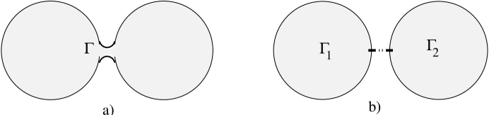
Figure 3: Manifold $\Gamma$ (Fig. 3a) is on the verge of splitting into two classically disconnected manifolds $\Gamma_{1}$ and $\Gamma_{2}$ (Fig. 3b). These two manifolds may be connected at the quantum level.

We have confirmed by some toy-model calculations that the near-pinching case (if the connecting “tube” between, say, two manifolds is not too long) does indeed lead to a spectral hierarchy. Let us also mention that a general theorem of Cheeger (see [28]) can be viewed as a (moral) confirmation of our conjecture. Indeed, this theorem says that a lower bound of the first eigenvalue is $\lambda_{1}\geq h^{2}/4$ where Cheeger’s constant $h$ is defined as the lower bound of the ratio $|S|/{\rm inf}(|\Gamma_{1}|,|\Gamma_{2}|)$ when $S$ runs over all closed submanifolds of $\Gamma$ (of dimension $d-1$) which partition $\Gamma$ into two open manifolds $\Gamma_{1},\Gamma_{2}$, with common boundary $\partial\Gamma_{1}=\partial\Gamma_{2}=S$. We use the notation $|\Gamma|$ to denote the (riemannian) volume of $\Gamma$. Note that $h$ has the dimension of an inverse length, and that “pinching” does indeed correspond to the case where $h\rightarrow 0$.

Physically, we can view the very light mode arising in a nearly pinched configuration $\Gamma_{1}\cup\{{\rm tube}\}\cup\Gamma_{2}$ as coming from the effect of a weak coupling between two “resonators” (or quantum mechanical systems) having regular spectra $\lambda_{n}^{(1)}$, $\lambda_{n}^{(2)}$. Before coupling, the ground state is degenerate, $\lambda_{0}^{(1)}=\lambda_{0}^{(2)}=0$. Weak coupling is generally expected to split this degeneracy into a doublet. As $\lambda_{0}=0$ is always an exact eigenvalue of the combined system (corresponding to $\phi_{0}(y)=1$), this mechanism always leads to a small $\lambda_{1}$ (going to zero with the coupling). Note that the eigenmode corresponding to $\lambda_{1}$ is approximately equal to $\phi_{1}(y)\simeq\varepsilon(y)$ where $\varepsilon(y)$ is $+1$ over $\Gamma_{1}$, and $-1$ over $\Gamma_{2}$.

We are aware of the fact that weakly coupled string theory suggests compactification on Ricci-flat manifolds (which exclude a spectral hierarchy). However, we think that string theory might still, in certain circumstances, allow for a spectral hierarchy: either because of $\alpha^{\prime}$-corrections to Einstein equations (which lead one away from the Ricci-flat case), or (more speculatively) because of conceivable quantum tunnelling effect between two (separate, but “near”) Ricci-flat manifolds $\Gamma_{1}$, $\Gamma_{2}$. Pictorially, such a tunnelling situation is the limit of Fig. 3b where the link between $\Gamma_{1}$ and $\Gamma_{2}$ is classically broken. The exponentially small coupling associated to such a tunnelling situation would naturally induce an exponentially small $\lambda_{1}$, and thereby a bigravity coupling scale $\mu$ exponentially smaller than the string scale.

3.3 Bigravity and Connes’ non-commutative geometry

Within his general non-commutative geometry programme [29], Connes introduced the model of a two-sheeted space $X$, made from the product of a continuous space $Y$ by a discrete “two-point space” $\{a,b\}$ (or $Z_{2}$) : $X=Y\times Z_{2}$. Though the algebra ${\cal A}$ of “functions on $X$” (defined as the algebra of pairs of functions viewed as diagonal matrices ${\rm diag}(f_{a}(y),f_{b}(y))$ with $y\in Y$) is commutative, the bimodule of 1-forms on such a space is not commutative [29]. Generalizations of this model (also based on the product of a continuum by a discrete space) were used in [30] to give a geometrical explanation of the structure of the Standard Model. In particular, it was found that the VEV of the Higgs field is related to the (non-commutative) “distance” between the two sheets. The metric aspect of such a two-sheeted space was developed along different lines by several authors [31], [32], [33], [34]. For instance, Ref. [31] introduced (non-commutative) analogues of the Riemannian metric, curvature tensor and scalar curvature, which enabled them to introduce a generalized Einstein-Hilbert action. This generalized Einstein-Hilbert action was found to contain (besides the standard integral of the scalar curvature of $Y$) a minimally coupled massless scalar field $\sigma$ related to the “distance” between the two sheets by $d\propto e^{-\sigma(y)}$. An alternative approach to studying gravitational effects within general non-commutative spaces has been proposed in [34]. We shall follow this approach which is based on a general “spectral action principle”. In its simplest form, this principle is proposing to take as bare bosonic (Euclidean) action for any non-commutative model $X$ the trace of the heat kernel associated with the square of the (non-commutative) Dirac operator $D_{X}$ of $X$:

$$I={\rm Tr}\,\exp\,(-t\,D_{X}^{2})\,.$$ (50)

Here $t\equiv m_{0}^{-2}$ introduces a cut-off, roughly equivalent to keeping only frequencies smaller than $m_{0}$. The cut-off-dependent Euclidean action (50) is viewed (à la Wilson) as the bare action at the mass scale $\sim m_{0}$.

It seems that all previous works interested in the metric aspect of a two-sheeted space $X=Y\times Z_{2}$ have restricted themselves (either for simplicity, or because of some constraints [33]) to the case where the metric is the same on the two sheets. By contrast, we focus here on the case where the two metrics are different, say $g_{\mu\nu}^{L}$ and $g_{\mu\nu}^{R}$, and the aim of this subsection is to compute the “potential” ${\cal V}(g_{L},g_{R})$ implied by the spectral action (50). Following Connes (see p. 569 of the English edition of his book [29]) we define a Dirac operator on a bi-Riemannian space $X=Y\times Z_{2}$ as

$$D_{X}=\left(\begin{array}[]{ccc}D\!\!\!\!/\,_{L}&&\gamma_{5}\,m\\ &&\\ \gamma_{5}\,m&&D\!\!\!\!/\,_{R}\\ \end{array}\right)\,.$$ (51)

This operator acts on bi-spinors $\left({\psi_{L}\atop\psi_{R}}\right)$ living on $Y\times Z_{2}$. Our conventions are that the (Euclidean) gamma matrices are hermitian, as well as $\gamma_{5}$ (which satisfies $\gamma_{5}^{2}=1$ and which anticommutes with the gamma matrices and therefore with the separate Dirac operators $D\!\!\!\!/\,_{L}$ and $D\!\!\!\!/\,_{R}$). The explicit form of the (hermitian) Dirac operators on each sheet is

$$D\!\!\!\!/\,_{L,R}=i\,\gamma^{\mu}_{L,R}\left(\partial_{\mu}+\Omega_{\mu}(L,R)\right),\quad\{\gamma^{\mu}_{I},\gamma^{\nu}_{I}\}=2\,g^{\mu\nu}_{I},\quad I=L,R\,.$$ (52)

The explicit form of the spin connections $\Omega_{\mu}$ will not be important for our calculations. On the other hand, the explicit form of the gamma matrices will be crucial. They read $\gamma_{L}^{\mu}=\gamma^{a}\,E_{aL}^{\mu}$, $\gamma_{R}^{\mu}=\gamma^{a}\,E_{aR}^{\mu}$ where $\{\gamma^{a},\gamma^{b}\}=2\,\delta^{ab}$ is a standard set of (space-independent) gamma matrices and where $E_{aL}^{\mu}(x)$, $E_{aR}^{\mu}(x)$ (where $x\in Y$) are vierbeins corresponding to the two positive definite metrics $g_{\mu\nu}^{L}$, $g_{\mu\nu}^{R}$ given on the abstract manifold $Y:g_{L}^{\mu\nu}(x)=\delta^{ab}\,E_{aL}^{\mu}\,E_{bL}^{\nu}$, etc. Note that the structure (51) assumes that we are given not only an identification map between corresponding points of the two sheets (here gauge-fixed by the identification of the two underlying abstract manifolds and the use of only one coordinate system $x^{\mu}$ to describe the metrics on the two sheets), but also a one-to-one map between the spin structures, and in particular between any choice of vierbein. In other words to any $E_{aL}^{\mu}$ must correspond a unique $E_{aR}^{\mu}$ so that an arbitrary, local SO(4) rotation of $E_{aL}^{\mu}$ corresponds to the same rotation of $E_{aR}^{\mu}$. It is most natural to use as map $E_{aL}^{\mu}\rightarrow E_{aR}^{\mu}$ the canonical map defined in [35]. This map can be defined by requiring that it reduces to simple rescalings $E_{aR}^{\mu}=e^{-\mu_{a}/2}\,E_{aL}^{\mu}$ when considering bi-orthogonal frames (as in Eq. (9) above). For simplicity, the quantity $m$ in Eq. (51) (which “connects” the two sheets) will be taken to be a constant real scalar. More generally, it could also be a matrix when considering multiplets of fermions and could be space-dependent. We shall see that $m$ is connected with the coupling scale $\mu$ in Eq. (6). It might be interesting to consider generalized models where $m$ (and therefore $\mu$) is linked to a fluctuating scalar $m(x)\propto e^{-\sigma(x)}$ as in [31].

The square of the Dirac operator (51) is easily obtained as

$$D_{X}^{2}=\left(\begin{array}[]{ccc}D\!\!\!\!/\,_{L}^{2}+m^{2}&&m\,\gamma_{5}(D\!\!\!\!/\,_{R}-D\!\!\!\!/\,_{L})\\ &&\\ m\,\gamma_{5}(D\!\!\!\!/\,_{L}-D\!\!\!\!/\,_{R})&&D\!\!\!\!/\,_{R}^{2}+m^{2}\\ \end{array}\right)$$ (53)

The heat kernel expansion of (50) is a series in increasing powers of $t=m_{0}^{-2}$ which starts at order $t^{-2}=m_{0}^{4}$. At this leading order the action $I$ leads to two bare cosmological constant terms $m_{0}^{4}/(4\pi^{2})\int d^{4}x(\sqrt{g_{L}}+\sqrt{g_{R}})$. At the next to leading order, ${\cal O}(t^{-1})={\cal O}(m_{0}^{2})$, one gets two separate Einstein actions $m_{0}^{2}/(48\pi^{2})\int d^{4}x(-\sqrt{g_{L}}\,R_{L}-\sqrt{g_{R}}\,R_{R})$ (with negative signs, as is appropriate for an Euclidean action $I_{E}$ which is essentially $I_{E}=-I_{\rm Minkowski}$ with a positive signature metric) as well as a “potential” term $+\int d^{4}x\,{\cal V}(g_{L},g_{R})$ proportional to $m_{0}^{2}\,m^{2}$. In view of its $m_{0}^{2}\,m^{2}$ scaling, the potential ${\cal V}$ contains no derivatives of $g_{L}$ or $g_{R}$. It can therefore be evaluated by considering the case of constant metrics $g_{\mu\nu}^{L}$, $g_{\mu\nu}^{R}$. We can then neglect the spin connections in (52) and go to the momentum representation $(i\,\partial_{\mu}\rightarrow k_{\mu})$ to set

$$D_{X}^{2}=\left(\begin{array}[]{ccc}k\!\!\!\!/\,_{L}^{2}+m^{2}&&m\,\gamma_{5}(k\!\!\!\!/\,_{R}-k\!\!\!\!/\,_{L})\\ &&\\ m\,\gamma_{5}(k\!\!\!\!/\,_{L}-k\!\!\!\!/\,_{R})&&k\!\!\!\!/\,_{R}^{2}+m^{2}\\ \end{array}\right)\,.$$ (54)

Here $k\!\!\!\!/\,_{L}\equiv\gamma_{L}^{\mu}\,k_{\mu}$, $k\!\!\!\!/\,_{R}\equiv\gamma_{R}^{\mu}\,k_{\mu}$. Using the explicit vierbein expressions of $\gamma_{L}^{\mu}$ and $\gamma_{R}^{\mu}$ we can rewrite these as $k\!\!\!\!/\,_{L}\equiv\gamma^{a}\,k_{a}^{L}$, $k\!\!\!\!/\,_{R}\equiv\gamma^{a}\,k_{a}^{R}$, where

$$k_{a}^{L}\equiv k_{\mu}\,E_{aL}^{\mu}\ ,\quad k_{a}^{R}\equiv k_{\mu}\,E_{aR}^{\mu}\,.$$ (55)

In terms of these two different vectors (that live in a local Euclidean space common to the tangent spaces of the two sheets), one easily finds that the eigenvalues of $D_{X}^{2}$ are

$$\lambda_{\pm}=\frac{\mbox{\boldmath$k$}_{L}^{2}+\mbox{\boldmath$k$}_{R}^{2}}{2}+m^{2}\pm\sqrt{\frac{(\mbox{\boldmath$k$}_{L}^{2}-\mbox{\boldmath$k$}_{R}^{2})^{2}}{4}+m^{2}(\mbox{\boldmath$k$}_{L}-\mbox{\boldmath$k$}_{R})^{2}}\,.$$ (56)

Here, all squares are evaluated with the flat Euclidean metric $\delta^{ab}$ appropriate to the local Euclidean space where both $k_{a}^{L}$ and $k_{a}^{R}$ live. In the limit $m^{2}\rightarrow 0$ (appropriate to the heat kernel expansion) the eigenvalues (56) read (we henceforth suppress the boldfacing of the Euclidean vectors $k^{L}$ and $k^{R}$)

$$\lambda_{+}=k_{L}^{2}+m^{2}+m^{2}\,\frac{(k_{L}-k_{R})^{2}}{k_{L}^{2}-k_{R}^{2}}+{\cal O}(m^{4})\,,$$

$$\lambda_{-}=k_{R}^{2}+m^{2}-m^{2}\,\frac{(k_{L}-k_{R})^{2}}{k_{L}^{2}-k_{R}^{2}}+{\cal O}(m^{4})\,.$$ (57)

The heat kernel action reads

$$I={\rm Tr}\,\exp\,(-t\,D_{X}^{2})=4\int d^{4}x\int\frac{d^{4}k}{(2\pi)^{4}}\ [e^{-t\lambda_{+}}+e^{-t\lambda_{-}}],$$ (58)

where the 4 comes from the trace in spinor space and where $d^{4}k$ is the fourfold integral over the covariant components $k_{\mu}$. Expanding (58) in powers of $m^{2}$ leads to the mixing term $+\,4\,m_{0}^{2}\,m^{2}\int d^{4}x$ $(V_{1}+V_{2})$ where

$$V_{1}=-t^{2}\int\frac{d^{4}k}{(2\pi)^{4}}\ \frac{e^{-tk_{L}^{2}}-e^{-tk_{R}^{2}}}{k_{L}^{2}-k_{R}^{2}}\,(k_{L}-k_{R})^{2}\,,$$ (59)

$$V_{2}=-t^{2}\int\frac{d^{4}k}{(2\pi)^{4}}\,(e^{-tk_{L}^{2}}+e^{-tk_{R}^{2}})\,.$$ (60)

After our factorization of $m_{0}^{2}=t^{-1}$ in front of $V_{1}$ and $V_{2}$, the expressions (59), (60) are easily seen to be $t$-independent. We can then evaluate them by setting, say, $t=1$ in them. Noting that $k_{L}^{2}=\delta^{ab}\,k_{a}^{L}\,k_{b}^{L}=g_{L}^{\mu\nu}\,k_{\mu}\,k_{\nu}$, etc., $V_{2}$ is easily evaluated:

$$V_{2}=-c_{4}((\det g_{L}^{\mu\nu})^{-\frac{1}{2}}+(\det g_{R}^{\mu\nu})^{-\frac{1}{2}})=-c_{4}(\sqrt{g_{L}}+\sqrt{g_{R}})$$ (61)

where $c_{4}\equiv(16\pi^{2})^{-1}$ and where $g_{L}\equiv\det g_{\mu\nu}^{L}=(\det g_{L}^{\mu\nu})^{-1}$. The potential $V_{1}$ is much more tricky. However, it can be nicely expressed by introducing a Schwinger-type parameter $\alpha$ (varying between 0 and 1) and by using the identity $(e^{-a}-e^{-b})/(a-b)\equiv-\int_{0}^{1}d\alpha\exp[-((1-\alpha)a+\alpha b)]$. This naturally leads to the introduction of a one-parameter family of metrics $g(\alpha)$ interpolating between $g_{L}$ and $g_{R}$ (reached, respectively, when $\alpha=0$ and $\alpha=1$). More precisely we define

$$g^{\mu\nu}(\alpha)\equiv(1-\alpha)\,g_{L}^{\mu\nu}+\alpha\,g_{R}^{\mu\nu}\,.$$ (62)

[Note that the “line” connecting $g_{L}$ to $g_{R}$ is “straight” when expressed in terms of contravariant metrics (which naturally appear in the squared Dirac operator $D^{2}=-g^{\mu\nu}\,\partial_{\mu\nu}=+\,g^{\mu\nu}\,k_{\mu}\,k_{\nu}$), but will become “curved” when expressed in terms of the covariant components $g_{\mu\nu}(\alpha)$.] In terms of the definition (62) (and the associated $g_{\mu\sigma}(\alpha)\,g^{\sigma\nu}(\alpha)=\delta_{\mu}^{\nu}$, $g(\alpha)\equiv\det g_{\mu\nu}(\alpha)\equiv(\det g^{\mu\nu}(\alpha))^{-1}$) we find that $V_{1}$ can be written as

$$V_{1}=+\frac{1}{2}\,c_{4}\,\Delta E_{a}^{\mu}\,\Delta E_{a}^{\nu}\int_{0}^{1}d\alpha\,\sqrt{g(\alpha)}\,g_{\mu\nu}(\alpha)\,,$$ (63)

where $\Delta E_{a}^{\mu}\equiv E_{aR}^{\mu}-E_{aL}^{\mu}$. Finally, the ${\cal O}(m^{2})$ piece of the Euclidean action (i.e. the “potential”, remembering that ${\cal L}_{\rm Eucl.}=-{\cal L}_{\rm Mink.}$) predicted by the non-commutative approach to two-sheeted spaces reads $+\int d^{4}x\,{\cal V}$ with

$${\cal V}=\frac{m_{0}^{2}\,m^{2}}{4\pi^{2}}\left[\frac{1}{2}\,\Delta E_{a}^{\mu}\,\Delta E_{a}^{\nu}\int_{0}^{1}d\alpha\,\sqrt{g(\alpha)}\,g_{\mu\nu}(\alpha)-\sqrt{g_{L}}-\sqrt{g_{R}}\right]\,.$$ (64)

The explicit evaluation of the $\alpha$-integral in (64) can be reduced to (incomplete) elliptic integrals. In fact, it can be reduced to the evaluation of the single integral

$$I(g_{L},g_{R})\equiv\int_{0}^{1}d\alpha\,\sqrt{g(\alpha)}=\int_{0}^{1}\frac{d\alpha}{\sqrt{\det((1-\alpha)\,g_{L}^{\mu\nu}+\alpha\,g_{R}^{\mu\nu})}}$$ (65)

by using the identity

$$\left(\frac{\partial}{\partial\,g_{L}^{\mu\nu}}+\frac{\partial}{\partial\,g_{R}^{\mu}}\right)I(g_{L},g_{R})=-\frac{1}{2}\int_{0}^{1}d\alpha\,\sqrt{g(\alpha)}\,g_{\mu\nu}(\alpha)\,.$$ (66)

When considering a bi-orthogonal frame, say with $E_{aL}^{\mu}={\rm diag}(e^{-\mu_{a}^{L}/2})$, $E_{aR}^{\mu}={\rm diag}(e^{-\mu_{a}^{R}/2})$ (so that $g_{\mu\nu}^{L}={\rm diag}(e^{+\mu_{a}^{L}})$, $g_{\mu\nu}^{R}={\rm diag}(e^{+\mu_{a}^{R}})$ and $g_{L}^{-1}\,g_{R}={\rm diag}(e^{\mu_{a}})$ with $\mu_{a}=\mu_{a}^{R}-\mu_{a}^{L}$) the integral (65) is a rather simple elliptic integral of the first kind which, in principle, can be explicitly expressed in terms of the eigenvalues $\lambda_{a}^{L,R}\equiv e^{\mu_{a}^{L,R}}$. Of more direct interest for us is the discussion of the “weak-excitation” limit of ${\cal V}$, i.e. the limit $\mu_{a}=\mu_{a}^{R}-\mu_{a}^{L}\rightarrow 0$, i.e. $(g_{L}^{-1}\,g_{R})_{\nu}^{\mu}=\delta_{\nu}^{\mu}+h_{\nu}^{\mu}$ with $h_{\nu}^{\mu}\rightarrow 0$. In this limit we find that ${\cal V}$ behaves as (with $\sigma_{1}=\Sigma\,\mu_{a}$, $\sigma_{2}=\Sigma\,\mu_{a}^{2}$ as above)

$${\cal V} \simeq \frac{m_{0}^{2}\,m^{2}}{4\pi^{2}}\,(g_{L}\,g_{R})^{\frac{1}{4}}\left(-2+\frac{\sigma_{2}}{8}-\frac{\sigma_{1}^{2}}{16}\right)$$ (67)

$$= \frac{m_{0}^{2}\,m^{2}}{4\pi^{2}}\,(g_{L}\,g_{R})^{\frac{1}{4}}\left(-2+\frac{1}{8}\,h_{\mu}^{\nu}\,h_{\nu}^{\mu}-\frac{1}{16}\,(h_{\mu}^{\nu})^{2}\right)\,.$$

Besides a negative $m^{2}$-dependent, contribution to the cosmological constant (which has anyway bare contributions ${\cal O}(m_{0}^{4})$), we see that we do not get a Pauli-Fierz-type mass term for weak excitations away from $g_{\mu\nu}^{L}=g_{\mu\nu}^{R}$. We get instead (remembering that the (bare) Planck mass is $M_{L}^{2}=M_{R}^{2}=m_{0}^{2}/(48\pi^{2})$) a mass term proportional to $m^{2}\left[h_{\mu}^{\nu}\,h_{\nu}^{\mu}-\frac{1}{2}\,(h_{\mu}^{\nu})^{2}\right]$. Such a mass term contains a scalar ghost, but has the virtue (contrary to the Pauli-Fierz one $\sim m^{2}\,[h_{\mu}^{\nu}\,h_{\nu}^{\mu}-(h_{\mu}^{\mu})^{2}]$) of exhibiting excellent continuity properties of the limit $m^{2}\rightarrow 0$ for all processes linked to the generation of gravitational fields by sources (see, e.g., Appendix C of [37] where it is easily seen that $\alpha=1/2$ leads to an Einstein-like propagator $h_{\mu\nu}\,T^{\mu\nu}\propto T^{\mu\nu}(\Box-m^{2})^{-1}\,\left(T_{\mu\nu}-\frac{1}{2}\,\eta_{\mu\nu}\,T\right)$).

4 Phenomenology of Multigravity

4.1 Bigravity, and bicosmology, versus massive gravity

There is quite a sizable (and somewhat confusing) literature about the “problems” raised by having either “massive gravity” (i.e. a kind of finite-range version of Einstein’s theory), or a “massive graviton” in addition to Einstein’s massless one. We leave to a future publication a detailed discussion of such issues, but wish to emphasize the fact that the change of paradigm, brought by focusing on a fully nonlinear bigravity theory, drastically modifies, in our opinion, the way one should view the traditional “problems” of massive gravity (in both senses recalled in the sentence above). One of the basic points is that many of the “problematic” issues (such as, unboundedness of the energy, singularity of the infinite-range limit) simply loose their meaning in a general bigravity setting. Indeed, these problematic issues make sense only for states (in some theories) which are, at least asymptotically, close to some trivial, Poincaré invariant background. We think that, even when considering formally “small” excitations above a trivial background state $g_{\mu\nu}^{L}(x)=g_{\mu\nu}^{R}(x)=\eta_{\mu\nu}$, the exact bigravity configurations will generically develop into full-blown “bi-cosmological” configurations with fields that grow so much (in time and/or in space) so as to be outside the usually considered domain of bi-asymptotically flat configurations containing localized excitations. Note that most of the results concerning the “discontinuity” of the $m^{2}\rightarrow 0$ limit [38], [39], [37] implicitly (or explicitly) assumed such a framework of asymptotically decaying perturbations of a (minimum energy) Poincaré invariant background. We think that, if one relaxes this asymptotic restriction, there exists a sector of bigravity theories which exhibits “physical continuity” for small $m^{2}$, at the cost of cosmological behaviour on large scales. Note that such a claim, while being consistent with the works [40, 41, 42] which found continuity of massive graviton interactions in maximally symmetric ((A)dS) cosmological backgrounds, is somewhat different from the claim of [43],[44]. Indeed, the latter claim seems to insist on a framework (and a language, like that of propagators, coupling and scattering states) which preassumes the restriction to localized excitations of a Poincaré-invariant vacuum, i.e. that the metrics under consideration are asymptotically flat. Leaving to a future publication a detailed discussion of the “discontinuity” issue, we shall content ourselves here to sketch the general dynamical structure à la Arnowitt-Deser-Misner (ADM) [36] of bigravity theories.

4.2 ADM analysis of bigravity theories

We consider a general bigravity action (6). Let us decompose the two spacetime metrics ${}^{4}g_{\mu\nu}^{L}$, ${}^{4}g_{\mu\nu}^{R}$ into the two lapses $N_{L}$, $N_{R}$ $(N_{L}\equiv(-\,^{4}g_{L}^{00})^{-\frac{1}{2}})$, the two shift vectors $N_{L}^{i}$, $N_{R}^{i}$ $(^{4}g_{ij}^{L}\,N_{L}^{j}\equiv\,^{4}g_{0i}^{L})$ and the two spatial metrics $g_{ij}^{L}$, $g_{ij}^{R}$ $(g_{ij}^{L}\equiv\,^{4}g_{ij}^{L})$. We have

$$ds_{L}^{2}=-N_{L}^{2}\,dt^{2}+g_{ij}^{L}(dx^{i}+N_{L}^{i}\,dt)(dx^{j}+N_{L}^{j}\,dt)\,,$$

$$ds_{R}^{2}=-N_{R}^{2}\,dt^{2}+g_{ij}^{R}(dx^{i}+N_{R}^{i}\,dt)(dx^{j}+N_{R}^{j}\,dt)\,.$$ (68)

After integration by parts, each separate “Left” or “Right” pieces of the action (6) reads (say for the Left piece)

$$I_{L}=\int dt\int d^{3}x\,(\pi_{L}^{ij}\,\dot{g}_{ij}^{L}+\Pi_{L}\,\dot{\Phi}_{L}-N_{L}\,H_{L}-N_{L}^{i}\,H_{i}^{L})$$ (69)

where $\pi_{L}^{ij}$ is the Left gravitational momentum density, $\Pi_{L}$ is a (generic) matter momentum density and where the left super-Hamiltonian, and super-momentum densities have the structure

$$H_{L}=\frac{1}{M_{L}^{2}}\ \frac{1}{\sqrt{g_{L}}}\left(\pi_{L}^{ij}\,\pi_{ij}^{L}-\frac{1}{2}\,\pi_{L}^{2}\right)-M_{L}^{2}\,\sqrt{g_{L}}\,R_{L}+H_{L}^{\rm matter}\,,$$ (70)

$$H_{i}^{L}=-2\ D_{j}^{L}\,\pi_{Li}^{j}+H_{i}^{L\,{\rm matter}}\,.$$ (71)

Let us now consider the interaction term $-(^{4}g_{L}\,^{4}g_{R})^{\frac{1}{4}}\,V(^{4}g_{L}^{-1}\,{}^{4}g_{R})$. Using the fact that the local scalar $V$ must be (in particular) invariant under transformations of the type $dt^{\prime}=\lambda\,dt$, $dx^{\prime i}=\Lambda_{j}^{i}(dx^{j}+v^{j}\,dt)$ one finds that it can only depend on the lapses and shifts through the combinations $N_{R}/N_{L}$ and $(N_{R}^{i}-N_{L}^{i})/\sqrt{N_{L}\,N_{R}}$. Let us then replace the 8 variables $N_{L}$, $N_{L}^{i}$, $N_{R}$, $N_{R}^{i}$ by the combinations

$$\overline{N}\equiv\sqrt{N_{R}\,N_{L}}\,,\ n\equiv\sqrt{\frac{N_{R}}{N_{L}}}\,,\ \overline{N}^{i}\equiv\frac{1}{2}\,(N_{R}^{i}+N_{L}^{i})\,,\ n^{i}\equiv\frac{N_{R}^{i}-N_{L}^{i}}{2\,\sqrt{N_{R}\,N_{L}}}\,.$$ (72)

With these definitions it is found that the total action reads

$$I=\int dt\int d^{3}x\,(\pi_{L}^{ij}\,\dot{g}_{ij}^{L}+\pi_{R}^{ij}\,\dot{g}_{ij}^{R}+\Pi_{L}\,\dot{\Phi}_{L}+\Pi_{R}\,\dot{\Phi}_{R}-{\cal H})$$ (73)

where the total Hamiltonian density reads (here and below $g_{ij}^{L}$, $g_{ij}^{R}$ are the spatial metrics and $g_{L}\equiv\det g_{ij}^{L}$, $g_{R}\equiv\det g_{ij}^{R}$)

$${\cal H}(\overline{N},\overline{N}^{i},n,n^{i},g_{L},\pi_{L},g_{R},\pi_{R},\Phi_{L},\Pi_{L},\Phi_{R},\Pi_{R})=\overline{N}\,\overline{H}+\overline{N}^{i}\,\overline{H}_{i}$$ (74)

where

$$\overline{H}(n,n^{i},g,\pi,\Phi,\Pi)=n^{-1}\,H_{L}+n\,H_{R}-n^{i}\,H_{i}^{L}+n^{i}\,H_{i}^{R}+(g_{L}\,g_{R})^{\frac{1}{4}}\,V(n,n^{i},g_{L},g_{R})\,,$$ (75)

$$\overline{H}_{i}(g,\pi,\Phi,\Pi)=H_{i}^{L}+H_{i}^{R}\,.$$ (76)

The crucial point for the present discussion is the separation of the 8 lapse and shift variables into two sets: (i) the four “average” lapse and shifts $\overline{N}$, $\overline{N}^{i}$, which are true Lagrange multipliers appearing only linearly in the action, and (ii) the four “relative” lapse and shifts $n$, $n^{i}$ which enter algebraically in the action (no kinetic terms) but in a non linear manner. The four average lapse and shifts give rise to four constraints, which are linked to the symmetry of the action under common diffeomorphisms:

$$\overline{H}=0\ ,\qquad\overline{H}_{i}=0\,.$$ (77)

$\overline{N}$, $\overline{N}^{i}$ are gauge variables which can be gauged away (e.g. to $\overline{N}=1$, $\overline{N}_{i}=0$). The four (first-class) constraints (77) can be used, together with the field equations (which involve $\overline{N}$ and $\overline{N}^{i}$) to eliminate four degrees of freedom (i.e. eight functions of positions and momenta). By contrast, the four relative lapse and shifts $n$, $n^{i}$ are not (undeterminable) gauge variables but are dynamical variables which are instantaneously determinable in terms of the other variables $(g,\pi,\Phi,\Pi)$ by their (algebraic) equations of motion:

$$\frac{\partial\,\overline{H}}{\partial\,n}=0\ ,\qquad\frac{\partial\,\overline{H}}{\partial\,n^{i}}=0\,.$$ (78)

This result generalizes the findings of [37] which studied the case of “massive gravity”, i.e. (21). We must assume here that the potential $V$ has a “good” dependence on $n$ and $n^{i}$ which allow for an (essential) unique solution of Eqs. (78) for a generic (or at least an open) domain of free dynamical data $g,\pi,\Phi,\Pi$. We think that the only (covariant) situation where $n$ and $n_{i}$ combine with $\overline{N}$, $\overline{N}^{i}$ to generate more (gauge-related) Lagrange multipliers is the case where ${\cal V}$ is linear in $N_{L}$ and $N_{R}$, which must then correspond (by covariance) to ${\cal V}=c_{L}\,N_{L}\,\sqrt{g_{L}}+c_{R}\,N_{R}\,\sqrt{g_{R}}=c_{L}(-\det\,^{4}g_{\mu\nu}^{L})^{1/2}+c_{R}(-\det\,^{4}g_{\mu\nu}^{R})^{1/2}$. For instance, we can think that $V(n,n_{i})$ contains terms quadratic in $n^{i}$ (as already follows from a Pauli-Fierz mass term), and behaves, for both large (respectively, small) $n$ as $+\,a\,n^{2}$ (respectively $+\,b\,n^{-2}$). Note also that if we define the new scalar potential $V^{\rm new}$ by factoring $(-\det\,^{4}g_{\mu\nu}^{L})^{1/2}+(-\det\,^{4}g_{\mu\nu}^{R})^{1/2}$ instead of $(^{4}g^{L}\,{}^{4}g^{R})^{1/4}$ from ${\cal V}$, i.e. ${\cal V}=((-\det\,^{4}g_{\mu\nu}^{L})^{1/2}+(-\det\,^{4}g_{\mu\nu}^{R})^{1/2})V^{\rm new}$, the last term in Eq. (75) will become $(n^{-1}\sqrt{g_{L}}+n\sqrt{g_{R}})V^{\rm new}(n,n_{i},g_{L},g_{R})$. It is then enough to require that $V^{new}(n)$ grows in any manner (even logarithmically) towards $+\infty$, as $n\rightarrow+\infty$ or $n\rightarrow 0$. Such conditions ensure the existence of (possibly non unique) solutions of the equations of motion of $n$ and $n^{i}$, Eq. (78).

We can then use (78) to eliminate $n$ and $n^{i}$ (by replacing them by their expression in terms of the other dynamical data). It is then easily seen that the reduced Hamiltonian $\overline{H}_{\rm red}(g,\pi,\Phi,\Pi)$ obtained by inserting these expressions into (75) defines (together with (76)) a dynamical system for the variables $g_{ij}^{L}$, $\pi_{L}^{ij}$, $g_{ij}^{R}$, $\pi_{R}^{ij}$, $\Phi_{L}$, $\Pi_{L}$, $\Phi_{R}$, $\Pi_{R}$ (submitted to the four first-class constraints (77) coming from the Lagrange multipliers $\overline{N}$, $\overline{N}^{i}$). For instance, if we consider the matter-free system, we end up with the $6+6$ degrees of freedom linked to $g_{ij}^{L}$ and $g_{ij}^{R}$, from which must be subtracted 4 degrees of freedom killed by the first-class constraints (77). This leaves us with 8 degrees of freedom. As in the analysis of (nonlinear) massive gravity in [37], which concluded to the presence of 6 degrees of freedom (instead of the expected 5 of a Pauli-Fierz linear graviton), we have here $2+6=8$ (where the 2 can be formally thought of as corresponding to an Einstein (massless) graviton, and the 6 to a “massive graviton”).

Two of the potential defects of the supplementary tensor degree of freedom ($1=6-5$) are, according to [37]: (i) the unboundedness of the total “energy”, and (ii) experimental difficulties (e.g. with light scattering by the Sun), even if a suitable mass term can be found for which the $m^{2}\rightarrow 0$ limit exists. Our point of view concerning (i) is to argue that the notion of energy is not defined when considering (as we argue must be done) non-asymptotically flat metrics, with cosmological-type behaviour at infinity. Alternatively, we can dismiss the problem of spatial boundary conditions by considering spatially compact manifolds (e.g. with toroidal topology). For such a situation, the dynamics associated to (73)–(78) should entail a well-defined (classical) evolution system for $g_{L},\pi_{L},g_{R},\pi_{R},\ldots$ The ill-defined issue of “unbounded energy” is then transformed in a well-posed dynamical question: do Hamilton’s equations of motion quickly lead to a catastrophic evolution towards some singular state?, or do they admit many solutions which evolve rather quietly on times scales comparable to the age of the universe? (which is the only stability property which is really required by experimental data). This question will be discussed in detail in [12]. Let us only mention here the result that there does exist, for suitable potentials ${\cal V}$, many solutions which can quietly evolve on Hubble time scales or more.

4.3 Phenomenology and a new form of dark energy

Using the dynamical, and cosmological like, viewpoint expressed in the previous subsection, let us now briefly discuss why we think that bigravity is not only compatible with existing gravitational data, but might also furnish a natural explanation of the recently observed cosmic acceleration. Let us first argue that there exist large classes of bigravity data $g_{L},\pi_{L},g_{R},\pi_{R},\ldots$ which can adequately represent the universe as we see it at the present moment. For definiteness, we assume that we “live on the right brane” (when viewed in brane language), i.e. that the matter around as is made of $\Phi_{R}$-type matter only. Let us start by considering an instantaneous “Einstein” model of our universe, i.e. an exact solution $g_{R},\pi_{R},\Phi_{R},\Pi_{R}$ of the constraints $H^{R}=0=H_{i}^{R}$. Let us complete this configuration by a random “Einstein” model of the (shadow) left universe, i.e. a solution $g_{L},\pi_{L},\Phi_{L},\Pi_{L}$ of $H^{L}=0=H_{i}^{L}$. Taken together, these two configurations “nearly” satisfy the bigravity constraints (77) and (78). More precisely, (77) is satisfied modulo a term proportional to $V$, while (78) is satisfied modulo terms proportional to $\partial V/\partial n$ and $\partial V/\partial n^{i}$. Let us assume that all dimensionless variables ($n$, $n^{i}$ and $g_{L}^{-1}\,g_{R}$) are of order unity, and that $V\propto\mu^{4}$ is at most comparable to the average cosmological energy density $V\sim 10^{-29}\,g\,{\rm cm}^{-3}$ (i.e. $\mu\sim 10^{-3}$ eV) (in right units, say). Instead of viewing Eqs. (78) as equations for determining $n$ and $n^{i}$, we can pick rather arbitrary (initial) values of $n$ and $n^{i}$ (or order unity) and slightly deform the Einstein data $g_{R},\pi_{R},\ldots,g_{L},\pi_{L},\ldots$ to compensate for the small violation of the usual Einstein constraints brought by the terms proportional to $V$, $\partial V/\partial n$ and $\partial V/\partial n^{i}$. It is intuitively clear that there are many ways of doing so, i.e. of constructing exact bigravity initial data $g_{R},\pi_{R},\ldots,g_{L},\pi_{L},\ldots$ which exactly satisfy (77) and (78) for arbitrarily given $n$ and $n^{i}$. Locally, say around our Galaxy, the new, deformed data $g_{R},\pi_{R},\ldots$ can be constructed so as to be experimentally indistinguishable from a pure Einstein model (after all, we are simply modifying the stress-energy tensor in the Galaxy by less than $10^{-29}\,g\,{\rm cm}^{-3}$, which is many orders of magnitude smaller than the average density in the Galaxy). If the dependence of $V$ on $n$ and $n^{i}$ is adequate the equations (78) will continue to admit a solution $(n,n^{i})$ during the future evolution of the other dynamical variables. In fact, as (under a general assumption made in Section 2 above) we know one exact (but physically trivial) solution of the full bigravity evolution equations, namely $g_{\mu\nu}^{L}(t,x)=g_{\mu\nu}^{R}(t,x)$, i.e. $g_{L}=g_{R}$, $\pi_{L}=\pi_{R}$, $\Phi_{L}=\Phi_{R},\ldots$ with $n=1$, $n^{i}=0$, we expect (by mathematical continuity) that there will be classes of bigravity solutions where, during a long time, $g_{L}\simeq g_{R}$, $\pi_{L}\simeq\pi_{R},\ldots$ with $n\simeq 1$, $n^{i}\simeq 0$. The crucial question is whether one can solve Eqs. (78) for a long time (without catastrophe) for more general data where $g_{L}^{-1}\,g_{R}={\cal O}(1)$ and $n={\cal O}(1)=n^{i}$. This question will be addressed in [12] for cosmological-type solutions and in [13] for solar-system-type solutions. Note that this is here that the potential “discontinuity” problems linked to the $m^{2}\rightarrow 0$ (or $\mu\rightarrow 0$) limit show up because the potential $V(n,n^{i})$ is proportional to $\mu^{4}$, so that, when solving for $n$ and $n^{i}$ Eqs. (78), $\mu^{4}$ will tend to appear in a denominator and might cause the solution $n,n^{i}$ to take parametrically large values, proportional to some negative power of $\mu$ (depending on the behaviour of, say, $V(n)$ as $n\rightarrow+\infty$ or $n\rightarrow 0$).

Assuming, for the time being, the continuous existence of regular bigravity solutions, evolved from some data $g_{L},\pi_{L},g_{R},\pi_{R},n,n^{i},\ldots$ we can finish by mentioning some of the pleasing phenomenological aspects of bigravity. First, bigravity exactly satisfies the equivalence principle, because each type of matter (say $\Phi_{R}$ whithin “our universe”) is universally coupled to the corresponding metric, say $g_{\mu\nu}^{R}$. Second, (as just discussed) there are classes of bigravity solutions which differ from standard Einstein ones only by the presence “on the right-hand side” of Einstein’s equations of numerically very small additional terms (say $t_{\mu\nu}^{R}\sim t_{\mu\nu}^{L}\sim 10^{-29}\,g\,{\rm cm}^{3}$ in the covariant form (14)), which locally modify $g_{\mu\nu}^{R}$ and $\Phi^{R}$ (and $g_{\mu\nu}^{L}$, $\Phi^{L}$) only in a numerically very small way (though they might globally forbid the stable existence of asymptotically flat models). These solutions will be fully compatible with all local (or quasi-local) experimental tests of relativistic gravity: such as solar-system tests and binary-pulsar tests. Third, if $\mu$ indeed happens to be of the order of $10^{-3}$ eV, and if $g_{L}^{-1}\,g_{R}$ is of order unity, bigravity will only lead to experimentally significant deviations from Einstein’s gravity on cosmological scales. Moreover, if, seen from our universe $g_{\mu\nu}^{R}$, we view $g_{\mu\nu}^{L}$ as an “external field”, or, more precisely, if we (approximately) view the “difference” between the two metrics $g_{L}^{-1}\,g_{R}$ as a given (time varying) tensor “condensate” of order unity, the potential term ${\cal V}=\sqrt{g_{R}}(g_{R}^{-1}\,g_{L})^{\frac{1}{4}}\,V(g_{L}^{-1}\,g_{R})$ can be approximately viewed as a time-varying “vacuum energy” term (of order $\mu^{4}$), i.e. as a kind of “dark energy”. It is tempting to assume that this new form of dark energy (which might be called “tensor quintessence”) can explain the observed cosmic acceleration. It might also be used in primordial cosmological scenarios, possibly when using the idea mentioned above that $\mu$ could be an evolving field. See [12] for a study of this new form of dark energy, and its phenomenological differences with quintessence models based on evolving scalar (rather than tensor) condensates.

5 Conclusions

In this paper we suggested a new paradigm concerning “massive gravity” and “large scale modification of gravity”. Considering the fully nonlinear bigravity action suggests to change viewpoint: instead of the theory with massless and massive graviton(s) we had in linearized approximation, we are dealing with several interacting metrics. We introduced the concept of universality class which we formulated using bigravity (two interacting metrics) as an example. Different approaches (brane, KK, non-commutative geometry) naturally lead to different universality classes for the fully nonlinear bigravity action. Another important new suggestion is that almost all solutions must now be of the non-asymptotically flat (cosmological) type.

This new formulation can change the standard problematic of the $m^{2}\rightarrow 0$ discontinuity. We showed the existence of classes of solutions that are compatible with “our universe”. However, we do not claim to have proven that general solutions of bigravity are phenomenologically acceptable. The two main problems of massive gravity (ghost, potential blow up of some field variables when $m^{2}\rightarrow 0$) must still be examined in detail. The important problem is to find the matching to the local sources of the field so that the full metric is free of singularities. We do not worry about matching at infinity because we abandon the requirement of asymptotic flatness. It is possible that in some models of bigravity such local matching does not exist because of the explicit or implicit presence of ghost modes in the theory. Such models would be physically unacceptable. We note in this respect that the 6-dimensional model discussed in [21] which does not contain negative tension branes, contains instead either branes with equations of state violating the weak energy condition $T_{\mu\nu}^{\rm brane}\,\ell^{\mu}\,\ell^{\nu}\geq 0$ ( with light-like $\ell^{\mu}$) or has a conifold singularity in the bulk. The physical consistency of this model must be further investigated. We have also quoted mathematical theorems linking the existence of a hierarchical spectrum (necessary for the derivation of an effective bigravity Lagrangian) to the necessary negativity of the Ricci curvature of the compactified manifold. This sign condition might hide the presence of ghost-like fields in the theory. These questions are pressing and deserve detailed investigation.

Assuming a positive resolution of these issues or simply taking the phenomenological viewpoint that nonlinear bigravity Lagrangians open an interesting new arena for non standard gravitational effects, we shall explore in future publications [12], [13] the nonlinear physics of bigravity actions, with a particular view on its cosmological aspects, as it may provide a natural candidate for some new type of “dark energy”.

Acknowledgments: We would like to thank P. Bérard, M. Berger, A. Connes, J. Fröhlich, M. Gromov, M. Kontsevitch, A. Papazoglou, G. Ross and A. Vainshtein for informative discussions. I.K. is supported in part by PPARC rolling grant PPA/G/O/1998/00567 and EC TMR grants HPRN-CT-2000-00152 and HRRN-CT-2000-00148.

Appendix

In this Appendix we check the consistency of the linearized limit of the nonlinear action (6) with a direct linearized analysis of the coupling strengths of massless and light graviton modes in brane models. Omitting the tensor structure (and considering only the relative coefficients between the various terms) the Lagrangian describing the coupling of the massless graviton mode $h^{0}$, and of the lightest one $h^{1}$, reads

$$L_{Lin}=h^{0}\partial^{2}h^{0}+h^{1}\left(\partial^{2}+m_{1}^{2}\right)h^{1}+\frac{1}{M_{p}}\left(h^{0}+\alpha_{L}h^{1}\right)T_{L}+\frac{1}{M_{p}}\left(h^{0}-\alpha_{R}h^{1}\right)T_{R}$$ (79)

where the coefficients $\alpha_{L,R}$ describe the relative strengths of the massive graviton coupling to the matter on left and right branes. It seems that there are four parameters here: $M_{p},\,m_{1},\,\alpha_{L},$ and $\alpha_{R}$.

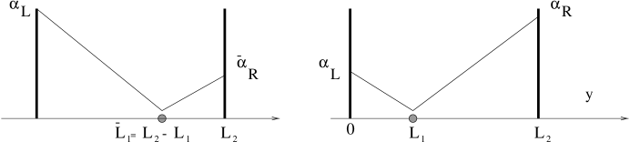
Figure 4: Here $L_{1}$ is the position of the bounce. The left configuration is just the mirror image of the right one and the positions of the bounces are related by $\bar{L}_{1}=L_{2}-L_{1}$. Under this transformation left and right branes are exchange their roles and, at the same time, $\alpha_{R}=\exp(2L_{1}-L_{2})\rightarrow\bar{\alpha}_{R}=\exp(2L_{2}-L_{1})=\alpha^{-1}_{R}$.

But actually $\alpha_{L}=\alpha_{R}^{-1}$ which is extremely important as we shall see next. This relation follows from the expression for $\alpha_{R}$ which was obtained in [1] (see Eq.(20) and Eq.(22) there)

$$\alpha_{R}=\exp\left(2L_{1}-L_{2}\right)\,.$$ (80)

Being derived originally for the $+-+$ model this expression holds for other models with bigravity, for example the $++$ model. In Figure 3 it is shown that one can interchange left and right branes by changing the position of the bounce from $L_{1}$ to $\bar{L}_{1}=L_{2}-L_{1}$. One gets the new coupling strength

$$\bar{\alpha}_{R}=\exp\left(2\bar{L}_{1}-L_{2}\right)=\exp\left(L_{2}-2L_{1}\right)=\frac{1}{\alpha_{R}}\,.$$ (81)

At the same time it is easy to see that a new right brane is just an old left one, so that we have the result

$$\alpha_{L}=\bar{\alpha}_{R}=\frac{1}{\alpha_{R}}\,.$$ (82)

This relation is crucial to the consistency of the nonlinear bigravity approach because only in this case can one relate $h_{0}$ and $h_{1}$ to $h_{L}\sim\left(h^{0}+\alpha_{L}h_{1}\right)$ and $h_{R}\sim\left(h^{0}-\alpha_{R}h_{1}\right)$ by orthogonal rotation. If it were not the case one would get mixing between $h_{L}$ and $h_{R}$ even in the limit $m_{1}=0$ and we could not have two non-interacting worlds. Introducing

$$h_{L}=\cos\theta h^{0}+\sin\theta h^{1},\,\,\,,h_{R}=\sin\theta h^{0}-\cos\theta h^{1}\,\,\,,\tan\theta=\alpha_{R}$$ (83)

we can rewrite (79) as

$$L_{Lin}=h_{L}\partial^{2}h_{L}+h_{R}\partial^{2}h_{R}+\frac{m_{1}^{2}}{M_{L}^{2}+M_{R}^{2}}\left(M_{L}h_{R}-M_{R}h_{L}\right)^{2}+\frac{1}{M_{L}}h_{L}T_{L}+\frac{1}{M_{R}}h_{R}T_{R}$$ (84)

where $M_{L}=M_{p}/\sqrt{1+\alpha^{2}},\,\,M_{R}=\alpha M_{p}/\sqrt{1+\alpha^{2}}$

Let us note that in the limit $L_{2}\rightarrow\infty$ both $\alpha_{L}$ and $M_{p}$ are divergent and $\alpha_{R}\rightarrow 0$. In this limit $M_{L}$ is finite and $M_{R}\rightarrow\infty$. The massless graviton $h_{R}$ becomes essentially a free sterile particle and decouples from the spectrum, while the massive graviton $h_{R}$ interacts with matter on the left brane only. Long range gravity completely decouples from the right brane.

Here we discussed the linearized bigravity lagrangian for flat branes, but one can get the same picture for $(A)dS$ branes. The limiting case $L_{2}\rightarrow\infty$ with corresponds to a single $AdS_{4}$ brane was considered in [20] (see also [14, 45, 46, 47]).

References

- [1] I. I. Kogan, S. Mouslopoulos, A. Papazoglou, G. G. Ross and J. Santiago, Nucl. Phys. B 584, 313 (2000) [hep-ph/9912552].
- [2] R. Gregory, V. A. Rubakov and S. M. Sibiryakov, Phys. Rev. Lett. 84, 5928 (2000) [hep-th/0002072].
- [3] I. I. Kogan and G. G. Ross, Phys. Lett. B 485, 255 (2000) [hep-th/0003074].
- [4] I. I. Kogan, S. Mouslopoulos, A. Papazoglou and G. G. Ross, Nucl. Phys. B 595, 225 (2001) [hep-th/0006030].
- [5] I. I. Kogan, arXiv:astro-ph/0108220.
- [6] A. Papazoglou, D.Phil. Thesis [arXiv:hep-ph/0112159].
- [7] I. I. Kogan, S. Mouslopoulos, A. Papazoglou and G. G. Ross, Nucl. Phys. B 615 (2001) 191 [arXiv:hep-ph/0107307].
- [8] C. Csaki, J. Erlich and T. J. Hollowood, Phys. Rev. Lett. 84 (2000) 5932 [hep-th/0002161].
- [9] G. Dvali, G. Gabadadze and M. Porrati, Phys. Lett. B 484, 112 (2000) [hep-th/0002190].
- [10] N. Boulanger, T. Damour, L. Gualtieri and M. Henneaux, Nucl. Phys. B 597 (2001) 127 [arXiv:hep-th/0007220]; arXiv:hep-th/0009109.
- [11] C. J. Isham, A. Salam and J. Strathdee, Phys. Rev. D 3 (1971) 867.
- [12] T. Damour, I. Kogan and A. Papazoglou, arXiv:hep-th/0206044.
- [13] T. Damour, I. Kogan and A. Papazoglou, work in progress
- [14] M. Porrati, arXiv:hep-th/0112166.
- [15] V. A. Rubakov, Phys. Usp. 44 (2001) 871 [Usp. Fiz. Nauk 171 (2001) 913] [arXiv:hep-ph/0104152].
- [16] M. Gogberashvili, Mod. Phys. Lett. A 14 (1999) 2025 [arXiv:hep-ph/9904383].
- [17] L. Randall and R. Sundrum, Phys. Rev. Lett. 83 (1999) 4690 [arXiv:hep-th/9906064].
- [18] C. Csaki, J. Erlich, T. J. Hollowood and Y. Shirman, Nucl. Phys. B 581 (2000) 309 [arXiv:hep-th/0001033].
- [19] I. I. Kogan, S. Mouslopoulos and A. Papazoglou, Phys. Lett. B 501, 140 (2001) [hep-th/0011141].
- [20] A. Karch and L. Randall, JHEP 0105 (2001) 008 [arXiv:hep-th/0011156].
- [21] I. I. Kogan, S. Mouslopoulos, A. Papazoglou and G. G. Ross, hep-th/0107086.
- [22] A. S. Gorsky and K. G. Selivanov, Phys. Lett. B 485 (2000) 271 [arXiv:hep-th/0005066]; arXiv:hep-th/0006044; arXiv:hep-th/0009207.
- [23] J. R. Ellis, N. E. Mavromatos and D. V. Nanopoulos, Phys. Rev. D 62 (2000) 084019 [arXiv:gr-qc/0006004]; G. K. Leontaris and N. E. Mavromatos, Phys. Rev. D 64 (2001) 024008 [arXiv:hep-th/0011102].
- [24] L. Pilo, R. Rattazzi and A. Zaffaroni, JHEP 0007 (2000) 056 [arXiv:hep-th/0004028]; I. I. Kogan, S. Mouslopoulos, A. Papazoglou and L. Pilo, Nucl. Phys. B 625 (2002) 179 [arXiv:hep-th/0105255].
- [25] W. D. Goldberger and M. B. Wise, Phys. Rev. Lett. 83 (1999) 4922 [arXiv:hep-ph/9907447].
- [26] P. Bérard, Spectral Geometry:Direct and Inverse Problems, Lecture Notes in Mathematics 1207 (Springer, Berlin, 1986).
- [27] M. Ledoux, Annales de la Faculté des Sciences de Toulouse, 9 (2000) 305.
- [28] M. Berger, P. Gauduchon and E. Mazet, Le Spectre d’une Variété Riemannienne , Lecture Notes in Mathematics 194 (Springer, Berlin, 1971); M. Berger, Riemannian Geometry Today: Introduction and Panorama (Springer, 2002, in press).
- [29] A. Connes, Inst.Hautes Études Sci. Publ. Math. 62 (1985) 257; Géométrie Non Commutative (InterEditions, Paris, 1990); Non Commutative Geometry (Academic Press, San Diego, 1994).
- [30] A. Connes and J. Lott, Nucl. Phys. Proc. Suppl. 18B (1991) 29.
- [31] A. H. Chamseddine, G. Felder and J. Fröhlich, Commun. Math. Phys. 155 (1993) 205 [arXiv:hep-th/9209044].
- [32] A. H. Chamseddine and J. Fröhlich, arXiv:hep-th/9307012.
- [33] A. H. Chamseddine, J. Fröhlich and O. Grandjean, J. Math. Phys. 36 (1995) 6255 [arXiv:hep-th/9503093].
- [34] A. H. Chamseddine and A. Connes, Commun. Math. Phys. 186 (1997) 731 [arXiv:hep-th/9606001]; Phys. Rev. Lett. 77 (1996) 4868 [arXiv:hep-th/9606056].
- [35] J. P. Bourguignon and P. Gauduchon, Commun. Math. Phys. 144 (1992) 581.
- [36] R. Arnowitt, S. Deser and C. W. Misner, in Gravitation: an introduction to current research, ed. by L. Witten (Wiley, New York, 1962), pp 227 -265.
- [37] D. G. Boulware and S. Deser, Phys. Rev. D 6, 3368 (1972).
- [38] H. van Dam and M. Veltman, Nucl. Phys. B 22, 397 (1970).
- [39] V.I. Zakharov, JETP Lett. 12 (1970) 312.
- [40] A. Higuchi, Nucl. Phys. B 325, 745 (1989).
- [41] I. I. Kogan, S. Mouslopoulos and A. Papazoglou, Phys. Lett. B 503 (2001) 173 [arXiv:hep-th/0011138].
- [42] M. Porrati, Phys. Lett. B 498 (2001) 92 [arXiv:hep-th/0011152].
- [43] A. I. Vainshtein, Phys. Lett. B 39 (1972) 393.
- [44] C. Deffayet, G. R. Dvali, G. Gabadadze and A. I. Vainshtein, Phys. Rev. D 65 (2002) 044026 [arXiv:hep-th/0106001].
- [45] M. Porrati, Phys. Rev. D 65 (2002) 044015 [arXiv:hep-th/0109017].
- [46] A. Miemiec, Fortsch. Phys. 49 (2001) 747 [arXiv:hep-th/0011160].
- [47] M. D. Schwartz, Phys. Lett. B 502 (2001) 223 [arXiv:hep-th/0011177].