hep-th/0206033

MCTP-02-26

Penrose Limits and RG Flows

Eric Gimon¹, Leopoldo A. Pando Zayas^1,2 and Jacob Sonnenschein^1,3

¹ School of Natural Sciences

Institute for Advanced Study

Princeton, NJ 08540

² Michigan Center for Theoretical Physics

Randall Laboratory of Physics, The University of Michigan

Ann Arbor, MI 48109-1120

³ School of Physics and Astronomy

Beverly and Raymond Sackler Faculty of Exact Sciences

Tel Aviv University, Ramat Aviv, 69978, Israel

The Penrose-Güven limit  simplifies a given supergravity solution into a pp-wave background. Aiming at clarifying its relation to renormalization group flow we study the Penrose-Güven limit  of supergravity backgrounds that are dual to non-conformal gauge theories. The resulting backgrounds fall in a class simple enough that the quantum particle is exactly solvable. We propose a map between the effective time-dependent quantum mechanical problem and the RG flow in the gauge theory. As a testing ground we consider explicitly two Penrose limits of the infrared fixed point of the Pilch-Warner solution. We analyze the corresponding gauge theory picture and write down the operators which are the duals of the low lying string states. We also address RG flows of a different nature by considering the Penrose-Güven limit  of a stack of $N$ $D_{p}$ branes. We note that in the far IR (for $p<3$ )the limit generically has negative mass². This phenomenon signals, in the world sheet picture, the necessity to transform to another description. In this regard, we consider explicitly the cases of $M2$ from $D2$ and $F1$ from $D1$ .

 

1 Introduction

In spite of the remarkable successes of the gauge/gravity duality [1], it has become clear that to penetrate to the core of the real world gauge dynamics, one will have to go beyond the SUGRA description and extract information from the related string theory. Superstring theories on backgrounds like the $AdS_{5}\times S^{5}$ are still far from being tractable. However, a breakthrough in turning the string theory into a solvable one, has been recently achieved [6] by taking the Penrose limit[2, 3] (see also [4, 5])in the neighborhood of a suitably selected null geodesic. This led to an exactly solvable superstring theory [7, 8]. In the SYM side of the duality relation this limit translates into a projection on operators with large R-charge $J$ such that $g_{YM}^{2}N\over J^{2}$ is fixed. So far most of the applications of the Penrose limit technique were on SUGRA backgrounds that are the holographic duals of conformal field theories. The gauge interactions that we detect in nature are characterized by a scale and hence are not conformaly invariant. Thus, a natural step to take is to apply the Penrose-Güven limit  on SUGRA backgrounds associated with non-conformal gauge theories.

Indeed, the goal of the present work is to analyze the pp–wave limit of SUGRA backgrounds that are dual to non-conformal field theories. Whereas in the context of the gauge/gravity duality the renormalization group flow was mapped into the variation of the SUGRA background fields, our main idea is to study the map between the field theory RG flow and the world-sheet time evolution of the corresponding string theory. We argue that the essential part of this map is in fact captured by the system of a quantum particle on the world-sheet(line) time-dependent pp–wave (tdppw) background. We show that this time-dependent quantum system can be solved exactly.

The best situation to develop our intuition is the flow between two fixed points. An example of a property of the RG flow of the gauge theory that might be computed in the QM system is the mixing between operators. Operators at the UV fixed point flow into the IR fixed point where they mix with several operators that carry their quantum numbers. In the dual QM system we can compute transition probabilities between initial state and final states of a time dependent QM harmonic oscillator. This yields the mixing between gauge theory states with short characteristic scales (UV) and gauge theory state with long characteristic scales (IR) which point to a mixing between operators in the UV and the IR which we still do not quite understand. The tdppw string theory generically differ from the conformal one in that it has additional non-trivial background fields like the dilaton, $NSNS$ $B_{\mu\nu}$ field and additional RR forms. We briefly discuss the effect of these fields.

We then demonstrate the general behavior of the tdppw duality in two classes of examples: (i) The Pilch Warner (PW) 10-d SUGRA solution [10] which is dual to the Leigh-Strassler flow [11] of a UV ${\cal N}=4$ SYM theory into an IR ${\cal N}=1$ superconformal YM theory. (ii) The near horizon limit of large $N$ $D_{p}$ branes [12]. In the former case we explicitly construct the Penrose limit of the IR fixed point of the PW solution. In fact we show that there are two possible natural limits that one can take. In the geometry side the two limits are associated with different choices of directions for the geodesic lines around which we zoom, whereas in the field theory side they are related to different sets of conformal operators that are the duals of the low lying string states. As opposed to the pp–wave limit of the ${\cal N}=4$ SYM here the string theory is characterized by non-trivial complex field-strength three form and hence a $B_{\mu\nu}$ term in the world action. Correctly matching to the field theory dynamics will require the inclusion of the effects of this B-field on the world sheet Hamiltonian.

For the second class of examples, the SUGRA backgrounds of large $N$ $D_{p}$ branes, we derive the explicit metric, dilaton and $p+2$ forms expressed in the Poincaré coordinates. An interesting result of these limits is the appearance of negative $\mu^{2}$ terms. We show that this is the generic behavior apart from certain small region of the radial coordinate. We discuss the meaning of these negative masses and show that the systems do not suffer from any pathological behavior. This is due to the fact that in the far IR one has to transform into another description of the system which is characterized by positive $\mu^{2}$ terms. In the case of $D_{1}$–brane in the region of large dilaton, an S-duality transformation render the system into that of large $N$ fundamental strings and for the case of $p=2$ the $D_{2}$ is replaced by an M2. In both cases the corresponding squared masses return to being positive. Thus changing our description of the Hilbert space of states fixes any pathological runaway behavior.

The analysis of Penrose limits of backgrounds dual to field theories that are not conformal was first addressed in [13], where the Schwarschild black hole in AdS, the small resolution of the conifold and the Klebanov-Tseytlin background were considered. Other papers that discussed related issues in pp-wave backgrounds [20]. The results of this paper were previously presented in [22]. While preparing the manuscript for submission we received [21] which overlaps with section 4 of our work.

In section 2 we discuss the general structure of the bosonic string on world-sheet time dependent pp–wave (tdppw) background. We start with the description of the geometry on the tdppw background, the additional forms and the dilaton and the relation between them via the SUGRA equation of motion. We then analyze the quantum particle on this background. Since this system is in fact identical to a set of harmonic oscillators with time dependent frequencies, we review some of the techniques for solving such systems. In particular we write down the Schroedinger wave function and certain transition probabilities. We show that the time-dependent frequencies associated with the tdppw limit have a form that enable us to have an exact solution to the QM system. We then briefly discuss the bosonic string on this background. Section 3 is devoted to a discussion of the RG flow of the gauge theory operators that associate with the tdppw limit. We review the operator/state duality of [6] and discuss its alteration for the tdppw cases. We adress the issue of the Calan Symazic equation and its stringy analog.

We then address our examples for the tdppw duality. We discussed our first example in section 4: the Penrose limits of the Pilch-Warner SUGRA solution that describes a RG flow from ${\cal N}=4$ to ${\cal N}=1$ SYM theories. We briefly review the the Pilch-Warner (PW ) solution. The Penrose limit at the UV fixed point is reduced to that of the ${\cal N}=4$ SYM discussed in [6]. We show that there are two different Penrose limits at the ${\cal N}=1$ fixed point which correspond to different geodesic lines. We analyze the associated string states and the corresponding gauge field operators. We also write an expression of the masses of the $AdS_{5}$ coordinates from the Penrose limit of the SUGRA flow in between the fixed points. The second class of examples are the pp–wave limit of the near horizon limit of the large number of $D_{p}$ branes are discussed in section 5. We perform the explicit limit in the Poincar’e coordinates and deduce the masses that appear in the string world sheet action. We show that apart from a small region of the radial coordinate, the values of $\mu_{u}^{2}$ are negative. The source of this behavior is the non-constant dilaton. We discuss the meaning of the negative world-sheet mass term for the propagating string. We analyze separately the cases of $p=1$ where there is a flow from $D1$ to $F1$ string as well as the flow form the $D_{2}$ solution to the uplifted $M2$ background. The masses in the proper IR picture turn out to be positive.

2 Strings on a time-dependent pp–wave background: General structure

2.1 The geometry of the pp-wave limit of non-conformal backgrounds

The general form of the pp–wave metric in the Brinkman coordinates is given by

$$ds^{2}=-4dx^{+}dx^{-}-\mu^{2}_{ij}(x^{+})x^{i}x^{j}(dx^{+})^{2}+dx^{i}dx^{i}$$ (2.1)

where $i,j=1...8$ This metric has an isometry group that includes the shift of $x^{-}$ and rotations in the eight dimensional space of $x^{i}$ which leave $\mu^{2}_{ij}$ invariant, for instance $SO(8)$ for $\mu^{2}_{ij}=\mu^{2}\delta_{ij}$. Isometry in a shift of $x^{+}$ occurs only provided that $\mu^{2}$ remains constant.

Any pp–wave metric can be achieved by taking the Penrose limit of a certain parent metric, as we discuss in appendix A. If the parent metric is conformaly invariant then the resulting $\mu^{2}_{ij}(x^{+})$ is a constant. For instance, in the $AdS_{5}\times S^{5}$ parent metric expressed in global coordinates, the daughter Killing vector is $\partial_{x^{+}}=\partial_{t}+\partial_{\psi}$ where $\partial_{t}$ is associated with conformal transformation and $\partial_{\psi}$ with R symmetry.

Non-conformal backgrounds expressed in terms of global coordinates are characterized by $G_{00}$ which is a function of time and hence shifting the global time $t$ is no longer a symmetry.

The curvature of the pp–wave metric is characterized by one non-trivial component of the Ricci tensor and vanishing scalar curvature.

$$R_{++}=Tr[\mu_{ij}^{2}(x^{+})]=\sum_{i}^{8}\mu_{i}^{2}(x^{+})\qquad R=0$$

where $\mu_{i}(x^{+})$ are the eigenvalues of $\mu_{ij}(x^{+})$.

In addition to the metric, the pp–wave background is characterized by a dilaton and certain forms. In the string frame the relation between the Ricci curvature, the dilaton and the five form is given by

$$R_{MN}=-2\nabla_{M}\nabla_{N}\phi+{1\over 96}e^{2\phi}[F_{M...}F_{N}^{...}-{1\over 10}G_{MN}F_{...}F^{...}]$$ (2.2)

where ${}_{...}\ ^{...}$ denotes contracted indices. Since only $R_{++}\neq 0$ this reduces to

$$R_{++}=-2\partial_{+}\partial_{+}\phi+{1\over 96}e^{2\phi}[F_{+...}F_{+...}].$$ (2.3)

In section 4 we will discuss a background that include also a three form. For that case one can easily amend (2.3).

2.2 The particle on the tdppw background

Prior to analyzing the bosonic string on the tdppw background, we start with the simpler case of a particle propagating on this background. The system is that of a set of harmonic oscillators with time-dependent frequencies. The corresponding classical action takes the form

$$S_{P}={1\over 2}\int d\tau[{1\over 2}((\dot{x}^{i})^{2}-\mu^{2}_{i}(\tau)(x^{2})]$$ (2.4)

where $\mu^{2}_{ij}$ has been taken to be diagonal. The classical equations of motion

$$\ddot{x}^{i}+\mu_{i}^{2}(\tau)x^{i}=0$$ (2.5)

are solved by

$$x^{i}=a^{i}v^{i}+{a^{i}}^{\dagger}{v^{i}}^{*}$$ (2.6)

where $v^{i}(t)$ has to obey

$$\ddot{v}^{i}+\mu_{i}^{2}(\tau)v^{i}=0$$ (2.7)

where there is no summation over the $i$ indices. The conjugate momenta are $p^{i}=a^{i}\dot{v}^{i}+{a^{i}}^{\dagger}\dot{v^{i}}^{*}$ and the Hamiltonian takes the form

$$H_{P}={1\over 2}[(p^{i})^{2}+\mu_{i}^{2}(\tau)(x^{i})^{2}]$$ (2.8)

We will now perform the canonical quantization of this system using two different methods. In the first one we elevate the classical $a$ and $a^{\dagger}$ into creation and annihilation operators $a$ and $a^{\dagger}$

$$a^{i}(\tau)=i[{v^{i}}^{*}(\tau)p^{i}(\tau)-\dot{v^{i}}^{*}(\tau)x^{i}(\tau)]\qquad{a^{i}}^{\dagger}=-i[v^{i}(\tau)p^{i}(\tau)-\dot{v}^{i}(\tau)x^{i}(\tau)]$$ (2.9)

To obey the standard quantization condition $[a^{i},{a^{j}}^{\dagger}]=\delta^{ij}$. one has to impose the following further condition on $v^{i}$

$$[\dot{v^{i}}^{*}v^{i}-\dot{v}^{i}{v^{i}}^{*}]=-i$$ (2.10)

The creation and annihilation operators are “time independent” since

$${da^{i}\over d\tau}={\partial a^{i}\over\partial\tau}+i[H(\tau),a^{i}(\tau)]=0$$ (2.11)

Thus we can now define a Fock space of states

$$a^{i}|0>=0;\qquad|n_{i}>={[{a^{i}}^{\dagger}]^{n}\over n!}|0>$$ (2.12)

In terms of $a$ and $a^{\dagger}$ the Hamiltonian takes the form

$$H_{P}={1\over 2}[((\dot{v}^{i})^{2}+\mu_{i}^{2}(v^{i})^{2})(a^{i})^{2}+((\dot{v^{i}}^{*})^{2}+\mu_{i}^{2}({v^{i}}^{*})^{2})({a^{i}}^{\dagger})^{2}+((|\dot{v}^{i}|)^{2}+\mu_{i}^{2}(|v^{i}|)^{2})({a^{i}}^{\dagger}a^{i}+a^{i}{a^{i}}^{\dagger})$$ (2.13)

For the special case of constant $\mu_{i}^{2}=w^{2}$ it is easy to check that $v^{i}(t)={e^{iw^{i}t}\over\sqrt{2w^{i}}}$ and then the Hamiltonian takes the usual form of $H={1\over 2}w^{i}({a^{i}}^{\dagger}a^{i}+a^{i}{a^{i}}^{\dagger})$ such that $H|n_{i}>=({1\over 2}+n_{i})w^{i}$.

The expectation values of the Hamiltonian at any time for the states $|n>$are

$$<n_{i}|H_{P}|n_{i}>=({1\over 2}+n_{i})[|\dot{v}^{i}(\tau)|^{2}+\mu_{i}^{2}(\tau)|v^{i}(\tau)|^{2}]$$ (2.14)

Note however that these states do not diagonalize the Hamiltonian. We will see shortly that one can define instead of the Hamiltonian another hermitian operator which is time independent and is diagonalized by (2.12). Meanwile we write the Schroedinger wave function of the $n_{i}$ state[17]

$$\Psi_{n_{i}}(x^{i},\tau)=\left[1\over 2\pi|v^{i}|^{2}\right]^{1/4}{1\over\sqrt{2^{n}_{i}n_{i}!}}\left[{v^{i}\over{v^{i}}^{*}}\right]H_{n_{i}}({x_{i}\over\sqrt{2|v_{i}|^{2}}})e^{i{\dot{v^{i}}^{*}\over{v^{i}}^{*}}x^{2}}$$ (2.15)

Consider the following invariant[19]

$$I={1\over 2}\left[{1\over|v|^{2}}x^{2}+(|v|p-|\dot{v}|x)^{2}\right]$$ (2.16)

where $v(\tau)=|v|(\tau)e^{-i\varphi(\tau)}$ was defined in(2.7). To simplify the notation we discuss from here on a single oscillator. It is easy to check that $I$ is hermitian and that it is an invariant, namely

$${dI\over d\tau}={\partial I\over\partial\tau}+i[H(\tau),I(\tau)]=0$$ (2.17)

We construct a new Fock space by using $\tilde{a}$ and $\tilde{a}^{\dagger}$ given by

$$\tilde{a}={1\over\sqrt{2}}\left[{1\over|v|}x+i(|v|p-|\dot{v}|x)\right]$$ (2.18)

which can easily be related to $a$, $a=\tilde{a}e^{i\varphi(\tau)}$. In terms of $\tilde{a}$ and $\tilde{a}^{\dagger}$ the invariant takes the form

$$I=\tilde{a}^{\dagger}\tilde{a}+{1\over 2}$$ (2.19)

such that the state $|\tilde{n}>={[{\tilde{a}}^{\dagger}]^{n}\over n!}|0>$ has an eigenvalue $I|\tilde{n}>=\lambda_{n}|\tilde{n}>=(n+1/2)|\tilde{n}>$ for the invariant $I$. Note that the invariant can also be expressed in the previous base since $I=a^{\dagger}a+1/2$. We can now expand the general solution of the Schrodinger equation in terms of the new base $|\tilde{n}>$.

$$\Psi=\sum_{\tilde{n}}c_{\tilde{n}}e^{i\alpha_{\tilde{n}}(\tau)}|\tilde{n}>$$ (2.20)

where $c_{\tilde{n}}$ are constants and $\alpha_{\tilde{n}}(\tau)=-(\tilde{n}+1/2)\int^{\tau}{dt^{\prime}\over|v(t^{\prime})|^{2}}$.

Of a particular interest for us will be the case where $\mu_{i}^{2}$ “flows” between two fixed points, constant $\mu^{(i)}$ at the initial time and constant $\mu^{(f)}$ at the final time. In that case there is a natural Fock space in both ends. To determine the transition between the initial and final states one can use the method of Bogolyubov transformation. Instead we follow the precedure of using the invariant. Suppose now that at $\tau=-\infty$ the Hamiltonian is characterized by a constant $\mu^{(i)}$ so that $|v(\tau=-\infty)|={1\over\sqrt{\mu^{(i)}}}$ and the system is in its ground state $|0,i>$. At $\tau\rightarrow\infty$ the corresponding “frequency” is $\mu^{(f)}$, and the system is at a state $|\tilde{n},f>$. At the final time $|v(\tau)|$ can be parametrized as follows $|v(\tau)|={1\over\sqrt{\mu^{(f)}}}[\cosh(\delta)+\sinh(\delta)\sin(2\mu^{(f)}\tau+\tilde{\delta})]^{1/2}$ where $\delta$ and $\tilde{\delta}$ are real. The transition probability between these initial and final states takes the form[19]

$$P_{0n}={(2n)!\over 2^{2n}(n!)^{2}}\left[{\cosh(\delta)-1\over(\cosh(\delta)+1)}\right]^{n/2}\left[{2\over(\cosh(\delta)+1)}\right]^{1/2}$$ (2.21)

for even $n$ and it vanishes for odd $n$. In the sudden approximation the transition probability takes the form

$$P_{0n}={(2n)!\over 2^{2n}(n!)^{2}}\left[{(\mu^{(f)}-\mu^{(i)})\over(\mu^{(f)}+\mu^{(i)}}\right]^{n/2}{2(\mu^{(f)}\mu^{(i)})^{1/2}\over\mu^{(i)}+\mu^{(f)}}$$ (2.22)

In certain cases it is useful to use the path-integral approach[18]. In this case the evolution of the wave function is expressed in terms of a Kernel $K(x^{\prime},\tau^{\prime};x,\tau)$ such that $\Psi(x,\tau)=\int dx^{\prime}K(x^{\prime},\tau^{\prime};x,\tau)$. The Kernel is determined by the path integral $K(x^{\prime},\tau^{\prime};x,\tau)=\int D(\tilde{x})e^{i\int_{\tau}^{\tau^{\prime}}Ld\tau^{\prime\prime}}$. An expression for the Kernel was written down in [18] and it takes the following form

$$K(x^{\prime},\tau^{\prime};x,\tau) = \left[{\sqrt{\dot{\varphi}^{\prime}\dot{\varphi}}\over 2\pi i\sin(\varphi^{\prime}-\varphi)}\right]^{1/2}e^{i/2({|\dot{v}|^{\prime}\over|v|^{\prime}}{x^{\prime}}^{2}-{|\dot{v}|\over|v|}x^{2})}$$ (2.24)

$$\times e^{\left({i\over 2\sin(\varphi^{\prime}-\varphi)}[\dot{\varphi}^{\prime}{x^{\prime}}^{2}+\dot{\varphi}{x}^{2})\cos(\varphi^{\prime}-\varphi)-2\sqrt{\dot{\varphi}^{\prime}\dot{\varphi}}{x^{\prime}}x]\right)}$$

where ^′ stands for a variable evaluated at $\tau^{\prime}$ and $\dot{A}\equiv\partial_{\tau}A$. It is easy to check that for constant $\mu$ where $|v|={1\over\sqrt{\mu}}$ and $\varphi=w\tau$ the Kernel reduces to that of an ordinary harmonic oscillator.

We can now apply these general considerations of a time dependent quantum Harmonic oscillator to the particular quantum mechanics on a tdppw backgrounds. It was shown in [4] ( see also appendix A) that a background with diagonal $\mu_{ij}^{2}$, the eigenvalues of the mass matrix take the following form

$$\mu_{i}^{2}(\tau)=-{\ddot{A}_{i}\over A_{i}}$$ (2.25)

where $A_{i}$ is given in terms of the metric. For instance in appendix A we have $A_{i}=\sqrt{g_{ii}}$ for $\mu_{x^{i}}$, and $A_{i}=\sqrt{E^{2}g_{\psi\psi}-\mu^{2}g_{tt}}$ for $\mu_{\phi}$. It is easy to see that $v_{i}(\tau)=A_{i}(\tau)$ is a solution of the defining equation (2.7). However since $v_{i}$ is in general complex and $A_{i}$ is real, it is clear that $v_{i}(\tau)=A_{i}(\tau)$ is not the most general solution. It is easy to show that the latter takes the form

$$v^{i}(\tau)=A_{i}(\tau)(c^{i}_{0}+c^{i}_{1}\int{d\tau\over A_{i}^{2}})\qquad({c^{i}}^{*}_{0}c^{i}_{1}-c^{i}_{0}{c^{i}}^{*}_{1})=i$$ (2.26)

where $c^{i}_{0}$ and $c^{i}_{1}$ are two time-independent complex coefficients and the condition they have to fulfill follows from (2.10). We would like to emphasize that the relation (2.9) implies that we have an exact solution of the quantum mechanical particle in the tdppw backgrounds we are considering. It is now straightforward to deduce the eigenvalues of the Hamiltonian (2.14), the Schroedinger wave function (2.15) and the transition probabilities (2.21) just by substituting (2.9) for $v(\tau)$.

The rate of change of the eigenvalues of the Hamiltonian in the basis (2.12)

$$\partial_{\tau}<n_{i}|H|n_{i}>=(n_{i}+1/2)\partial_{\tau}\mu_{i}^{2}(\tau)|v(\tau)|^{2}\sim[(c_{0}+c_{1}\int{d\tau\over A_{i}^{2}}]^{2}(\partial_{\tau}^{3}A_{i}A_{i}-\partial_{\tau}^{2}A_{i}\partial_{\tau}A_{i})$$ (2.27)

It is thus clear that the Hamiltonian has fixed points at

$$\partial_{\tau}^{3}A_{i}A_{i}-\partial_{\tau}^{2}A_{i}\partial_{\tau}A_{i}=0$$ (2.28)

This is clearly the same as demanding that $\mu$ be constant in eq. (2.25).

We will be interested in cases where there is a fixed point at each end of the flow, namely, when (2.28) is obeyed for $A_{i}(\pm\infty)$.

2.3 The bosonic tdppw string

The discussion of the particle in the previous subsection applies also to the zero modes of the corresponding bosonic string on tdppw background. In fact, as will be shown below, in the dual gauge theory picture the operators that correspond to the ground state and to the zero mode of the string are the basic building blocks of for the operators which are dual to the string states, and hence the quantum mechanical system captures the essence of the state/operator duality. In this subsection we add several comments about the full bosonic string theory. For the case where $\mu^{2}_{ij}(x^{+})$ is a constant matrix the string theory has been analyzed in [7, 8]. Here we focus on the properties that are directly related to non-constant masses and to additional fields of the background.

The action of the bosonic part of the superstring theory defined on a ppw background is given by

$$S = {1\over 2\pi\alpha^{\prime}}\int d^{2}\sigma\sqrt{h}[h^{\alpha\beta}(-4\partial_{\alpha}x^{+}\partial_{\beta}x^{-}-\mu^{2}_{ij}(x^{+})x^{i}x^{j}\partial_{\alpha}x^{+}\partial_{\beta}x^{+}+\partial_{\alpha}x^{i}\partial_{\beta}x^{i})+\alpha^{\prime}R^{(2)}\phi(x^{+})]$$ (2.30)

$$+ {1\over 2\pi\alpha^{\prime}}\int d^{2}\sigma\epsilon^{\alpha\beta}(B_{ij}(x^{+})\partial_{\alpha}x^{i}\partial_{\beta}x^{i}+B_{i+}(x^{j})\partial_{\alpha}x^{i}\partial_{\beta}x^{+})$$

For the case where the dilaton is a constant, the last term in the first line is just a constant times the Euler number of the world sheet and can be ignored. In general the dilaton term is multiplied by $\alpha^{\prime}$ and hence it is a quantum correction that does not directly affect the equations of motion. The $NS$–$NS$ $B_{\mu\nu}$ two form term will be relevant in section 4. In fact using a gauge transformation the $B_{\mu\nu}$ term transforms in such a way that it contains only a $B_{ij}(x^{+})$ component. This is in accordance with the general form of the pp–wave limit where any field strength has the form $F_{p+1}=dx^{+}\wedge\partial_{x^{+}}A_{p}(x^{+})$  [4]. However as will be discussed in section 4. the gauge transformation may yield a non-trivial surface term.

We now implement the light-cone gauge fixing. In [16] it was shown that the ppw background is the only curved space-time for which the gauge can be implemented as in the flat case namely $\sqrt{h}h^{\alpha\beta}=\eta^{\alpha\beta}$ with $h^{00}=-1$ . In addition, since $x^{+}$ obeys the equation $\Box x^{+}=0$ due to the equation of motion for $x^{-}$, we fix the residual symmetry by setting $x^{+}(\tau,\sigma)=\tau$. The gauged fixed action (for a constant dilaton) thus takes the form

$$S_{B}={1\over 2\pi\alpha^{\prime}}\int d\tau\int_{0}^{2\pi\alpha^{\prime}p^{+}}d\sigma[((\dot{x}^{i})^{2}-({x^{i}}^{\prime})^{2}-\mu^{2}_{ij}(\tau)x^{i}x^{j}+B_{ij}(x^{+})(\dot{x}^{i}{x^{j}}^{\prime}-\dot{x}^{j}{x^{i}}^{\prime})+B_{i+}(x^{j}){x^{i}}^{\prime}]$$ (2.31)

where ^′ stands for derivative with respect to $\sigma$. For the case of vanishing $B_{\mu\nu}$ terms we have a 1+1 dimensional action of eight scalar fields with a time-dependent mass term. Note also that if one reduce the world-sheet into a world-line going from the string model to a particle model the $B_{\mu\nu}$ terms do not affect the QM picture so the discussion of the previous subsection remains valid.

The corresponding equations of motion take the form

$$\ddot{x}^{i}-{x^{i}}^{\prime\prime}+\mu_{ij}(\tau)x^{j}-H_{+ij}(\tau){x^{j}}^{\prime}=0$$ (2.32)

where $H_{+ij}=\partial_{x^{+}}B_{ij}$ Unlike the quantum mechanical problem, even with a vanishing $H_{+ij}$ we cannot write down a universal solution to the equations of motion. If we substitute $\mu_{i}^{2}(\tau)=-{\ddot{A}_{i}\over A_{i}}$ and assuming a dependence on $\sigma$ of the form $e^{ik_{n}\sigma}$ we get an equation of the form $\ddot{x}^{i}+(k_{n}^{2}-{\ddot{A}_{i}\over A_{i}})x^{i}=$ which does not see to admit a universal solution.

The bosonic part of the world sheet Hamiltonian $H$ associated with the action 2.31 is given by

$$H=\int_{0}^{2\pi\alpha^{\prime}p^{+}}d\sigma[(p_{i}-B_{ij}(\tau){x^{j}}^{\prime})^{2}+({x^{i}}^{\prime})^{2}+\sum_{i}\mu^{2}_{i}(\tau){x^{i}}^{2}]$$ (2.33)

Obviously this Hamiltonian is not conserved due to the $\tau$ dependence of the mass term and the $B_{ij}$ term. We quantize the system following similar steps to those taken for the the particle.

3 The RG flow in the dual field theories

In [6] the field theory duals of the pp–wave string states were identified with operators of large $J$. In particular the vacuum state $|0,p^{+}>$ is identified with the state dual to the operator ${1\over\sqrt{J}N^{J/2}}Tr[Z^{J}]$ integrated over $S^{3}$ and an excited string state ${a^{i}}^{\dagger}_{n}{a^{j}}^{\dagger}_{-n}|0>$ with a state dual to

$$O_{n}={1\over\sqrt{JN^{J+2}}}\sum_{l=0}^{J}e^{2\pi iln/J}Tr[\phi^{i}Z^{l-J}\phi^{j}Z^{l}],$$ (3.1)

also integrated over $S^{3}$. In fact, as was mentioned above, the basic building blocks are the GS and the first excited states with $n=0$. It was further shown that the perturbative calculation with ${\lambda n^{2}\over J^{2}}$ as the coupling constant reproduced the string theory spectrum. The world-sheet energy eigenvalues $w_{n}=\sqrt{1+{\lambda n^{2}\over J^{2}}}$ are mapped into the values of $(\Delta-J)_{n}$ of the corresponding operators.

Throughout this work, the conformal nature of ${\cal N}=4$ SYM was explicitly used to map from the field theory on $R^{1,3}$ to a theory on $R\times S^{3}$ where the operator/state correspondence makes sense. To be more precise, suppose we start with a state $|\Psi(t,\vec{x})>$ in a conformal theory on ${R}^{1,3}$. We can use a conformal transformation to turn this into a state $|\Psi(t,\vec{\varphi})>$ on ${R}\times S^{3}$. After a Euclidean continuation, one can see that these states correspond to placing and operator $\Phi$ at the origin of ${R}^{4}$ and then using radial quantization to get $|\Psi(\lambda,\vec{\varphi})>$.

A natural question to ask is what of the structure of the BMN limit also holds for non-conformal cases and to what extent can the behavior of strings on a tdppw background teach us about the properties of the RG flow of the gauge theory dual to the tdppw background’s parent SUGRA solution. States in the tdppw correspond to states in the SUGRA solution localized around a geodesic in the Poincaré patch going from large values of $u$ (UV) to smaller values of $u$ as $t\to\pm\infty$. In the dual gauge theory we will start with a state, $|\Psi(t=0,\vec{x})>$, with short characteristic scales (UV) and it will evolve with time into a state,$|\Psi(t\gg 0,\vec{x})>$, with long characteristic scales(IR). Suppose we are dealing with a gauge theory which is conformal in the IR and the UV. Then near $t=0$ and $t\to\pm\infty$ we can use a separate state/operator map to get operators $\Phi_{UV}$ and $\Phi_{IR}$ respectively. The time evolution of $|\Psi(t,\vec{x})>$ which is described by strings on the tdppw background should correspond to some kind of RG-flow on the operator $\Phi$.

Going back briefly to the ${\cal N}=4$ case in [6], it was shown that an eigenvalue of the world sheet Hamiltonian $H_{ws}\equiv 2P^{-}$ for a given state translates in the CFT picture to $\Delta-J$ of the corresponding operator, where $\Delta$ is the conformal dimension and $J$ is a global symmetry charge. In the non-conformal case the analog of the time-dependence of the string Hamiltonian is the evolution of the gauge theory states in a scale dependent theory. Near conformal points, this is just scale dependence for conformal dimensions. Strictly speaking it does not make sense to discuss the eigenvalues of a time dependent Hamiltonian just as it is not meaningful to discuss conformal dimension in a non-conformal invariant system. In time-dependent QM, what replaces a description in terms of eigenstates of the Hamiltonian is the evolution of the wave-function determined by the Schroedinger operator $i\partial_{\tau}-H(\tau)$. In non-conformal field theories the RG flow is described by the Callan Symanzic (CS) equation which reads $({\cal M}\partial_{{\cal M}}+\beta\partial_{g}+n\gamma)G_{n}(x_{1},...x_{n},{\cal M})$ where ${\cal M}$ is the scale of the system (Euclidean time), $\beta$ is the $\beta$ function of the coupling $g$, $\gamma$ is the anomalous dimension of the operator and $G_{n}$ is an n-point function which depends on the locations of the operators and the scale. It is not completely clear to us how the RG flow for operators is related to the time evolution of the corresponding gauge theory states, but the connection is tantalizing.

The flow that will capture great part of our attention is between a fixed point in the UV and a fixed point in the IR, where the state/operator map can be well defined at both ends. An example of this nature will be discussed in details in section 4. A schematic description of the evolution of the conformal dimension is drawn in fig. 1. An operator that flows from the UV fixed point will mix with a set of operators in the IR that carry the same quantum numbers. The transition probabilities between the initial operator and the final ones maps into the transition probability of an initial state of the QM system described in the previous section to mix with certain final states.

Flows in gauge dynamical systems can take a variety of forms. In ordinary QCD there is a flow from asymptotic freedom in the UV to a mass gap in the IR. There is a state/operator map in the UV, and we could hope that a pp–wave–like procedure might show how states created by higher spin operators in the UV mix with infrared states like baryons.

4 The Penrose-Güven limit  of the Pilch-Warner solution

The Pilch-Warner solution computed in ref.[10] is one of the premier examples of the RG flow in the AdS/CFT context. It is the full ten dimensional supergravity uplift of the FGPW solution [9] describing the gravity dual of ${\cal N}=4$ supersymmetric $SU(N)$ Yang–Mills theory mass deformed to become the Leigh-Strassler ${\cal N}=1$ SCFT in the IR[11].

4.1 The Pilch-Warner solution-a brief review

The ten dimensional solutions computed in ref.[10] may be written as  :

$$ds^{2}_{10}=\Omega^{2}ds^{2}_{1,4}+ds^{2}_{5}\ ,$$ (4.1)

for the Einstein metric, where

$$ds^{2}_{1,4}=e^{2A(r)}\left(-dt^{2}+dx_{1}^{2}+dx_{2}^{2}+dx_{3}^{2}\right)+dr^{2}\,$$ (4.2)

and

$$ds_{5}^{2} = {L^{2}}{\Omega^{2}\over{\bar{\rho}}^{2}\cosh^{2}\chi}\left[{d\theta^{2}}+{\bar{\rho}}^{6}\cos^{2}\theta\left({\cosh\chi\over{4\bar{X}}_{2}}\sigma_{3}^{2}+{\sigma_{1}^{2}+\sigma_{2}^{2}\over{4\bar{X}}_{1}}\right)\right.$$ (4.3)

$$\left.+{{\bar{X}}_{2}\cosh\chi\sin^{2}\theta\over{\bar{X}}^{2}_{1}}\left({d\psi}+{{\bar{\rho}}^{6}\sinh\chi\tanh\chi\cos^{2}\theta\over{2\bar{X}}_{2}}\sigma_{3}\right)^{2}\right]\ ,$$

with

$$\Omega^{2} = {{\bar{X}}_{1}^{1/2}\cosh\chi\over{\bar{\rho}}}$$

$${\bar{X}}_{1} = \cos^{2}\theta+{\bar{\rho}}^{6}\sin^{2}\theta$$

$${\bar{X}}_{2} = {\rm sech}\chi\cos^{2}\theta+{\bar{\rho}}^{6}\cosh\chi\sin^{2}\theta\ .$$ (4.4)

The $\sigma_{i}$ are the standard $SU(2)$ left–invariant forms, the sum of the squares of which give the standard metric on a round three–sphere of radius 2. They are normalized such that $d\sigma_{i}={1\over 2}\,\epsilon_{ijk}\sigma_{j}\wedge\sigma_{k}$. We use the coordinates on the $S^{3}$ as $(\phi_{1},\theta_{1},\psi_{1})$ and we will us the explicit form for the $\sigma^{i}$’s:

$$\sigma_{1}+i\sigma_{2}=e^{i\phi_{1}}(d\theta_{1}-i\sin\theta_{1}d\psi_{1}),\qquad\sigma_{3}=d\phi_{1}+\cos\theta_{1}d\psi_{1}.$$ (4.5)

The functions ${\bar{\rho}}(r)$ and $\chi(r)$ which appear here in the ten dimensional metric are a one–parameter family of functions which depend on the size of the initial mass deformation.

At $r\to\infty$, the UV, the various functions in the solution have the following asymptotic values:

$${\bar{\rho}}(r)\to 1\ ,\,\,\chi(r)\to 0\ ,\,\,A(r)\to{r\over L}\ .$$ (4.6)

This gives standard AdS${}_{5}\times S^{5}$ with radius $L$. At $r\to\ 0$, the IR, we get new asymptotic values:

$${\bar{\rho}}(r)\to 2^{1\over 6}\ ,\,\,\sinh\chi(r)\to 3^{-{1\over 2}}\ ,\,\,A(r)\to{r\over\tilde{L}}\ .$$ (4.7)

(with ${\bar{\rho}}^{\prime}=\chi^{\prime}=A^{\prime\prime}=0$. This yields AdS₅ with a new radius $\tilde{L}=32^{-{5\over 3}}L$ times a deformed $S^{5}$ (see [24]). There is no known exact solution for the particular equations which give ${\bar{\rho}}(r),\chi(r)$ and $A(r)$ throughout the flow.

4.2 Penrose Limit of the Pilch-Warner solution in the IR

In the IR limit the Pilch-Warner solution has three simple Penrose limits that we can identify. In the first limit we pick a trajectory on $S^{5}$ near $\theta={\pi\over 2}$ and along the $-\,\psi$ direction (i.e., $\psi=-\textrm{const.}\,\cdot\,x^{+}+\ldots$), expanding to quadratic order in $\theta^{\prime}$: $\theta={\pi\over 2}-\theta^{\prime}$. The PW solution then takes the form:

$$ds_{10}^{2} = \Omega^{2}{9L^{2}\over 2^{10/3}}\bigg{[}-\cosh^{2}\rho d\tau^{2}+d\rho^{2}+\sinh^{2}\rho\,\,d\Omega_{3}^{2}\bigg{]}+L^{2}ds_{5}^{2},$$

$$ds_{5}^{2} = {\sqrt{3}\over 2}\bigg{[}\,d\theta^{\prime 2}+{\theta^{\prime 2}\over 4}(d\theta_{1}^{2}+d\phi_{1}^{2}+d\psi_{1}^{2}+2\cos\theta_{1}d\phi_{1}d\psi_{1})+({2\over 3}-{7\over 12}\,\theta^{\prime 2})d\psi^{2}$$

$$\qquad\quad+{\theta^{\prime 2}\over 6}(d\phi_{1}+\cos\theta_{1}d\psi_{1})d\psi\bigg{]},$$

$$\Omega^{2} = {2^{4/3}\over\sqrt{3}}-{\theta^{\prime 2}\over 2^{2/3}\sqrt{3}}.$$ (4.8)

If we now make the following coordinate transformation (the shift in in $\phi_{1}$ is not a change in the geodesic, but an $x^{+}$–dependent rotation of its transverse space):

$$x^{+}={\sqrt{3}\over 4\mu}(\tau-{2\over 3}\,\psi),\;x^{-}=\mu{L^{2}\over 2}({3\over 2}\,\tau+\psi),\;\hat{\phi_{1}}=\phi_{1}+{1\over 3}\,\psi,\;\theta^{\prime 2}={2\,y^{2}\over\sqrt{3}L^{2}},\;\rho^{2}={4\,r^{2}\over 3\sqrt{3}L^{2}}$$ (4.9)

we get the final form for the Penrose limit of the Pilch-Warner background :

$$ds^{2}_{PP} = -4dx^{+}dx^{-}-{4\over 3}\mu[\vec{r}^{2}+\vec{y}^{2}](dx^{+})^{2}+(d\vec{r})^{2}+(d\vec{y})^{2}+\emph{O}\,(L^{-1})$$

$${\cal A}_{(2)} = B_{NS-NS}+iB_{RR}$$ (4.10)

$$= -{\sqrt{3}\over 2}\,e^{i{2\over\sqrt{3}}\mu x^{+}}d\bar{z}_{1}\wedge d\bar{z}_{2}+{1\over\sqrt{6}}\,d\bigg{[}e^{i{2\over\sqrt{3}}\mu x^{+}}(\bar{z}_{1}\wedge d\bar{z}_{2}-\bar{z}_{2}\wedge d\bar{z}_{1})\bigg{]}$$

with $z_{1}=y_{1}+iy_{2},z_{2}=y_{3}+iy_{4}$ (the total derivative in ${\cal A}_{(2)}$ is important because it does not appear in the UV) and

$$p_{+} = \partial_{x^{+}}={2\over\sqrt{3}}\mu\,(\partial_{\tau}-{3\over 2}\,\partial_{\psi}+{1\over 2}\,\partial_{\psi_{1}})$$

$$p_{-} = \partial_{x^{-}}=\;\,{2\over 3\mu}\;(\partial_{\tau}+{3\over 2}\,\partial_{\psi}-{1\over 2}\,\partial_{\psi_{1}}).$$ (4.11)

The second and third limit correspond to boosting along a path in $S^{5}$ corresponding to $\theta=0,\;\theta_{1}=0$ or $\pi$. These two limits are pretty much identical except for a change in the sign of $\psi_{1}$. Expanding the PW solution to quadratic order in $\theta$ and $\theta_{1}$ we get:

$$ds_{10}^{2} = \Omega^{2}{9L^{2}\over 2^{10/3}}\bigg{[}-\cosh^{2}\rho d\tau^{2}+d\rho^{2}+\sinh^{2}\rho\,\,d\Omega_{3}^{2}\bigg{]}+L^{2}ds_{5}^{2},$$

$$ds_{5}^{2} = {\sqrt{6}\over 4}(1+{1\over 2}\theta^{2})\bigg{[}\,d\theta^{2}+{2\over 3}(1-{8\over 3}\theta^{2})(d\phi_{1}^{2}+d\psi_{1}^{2}-\theta_{1}^{2}d\phi_{1}\psi_{1}-\theta_{1}^{2}d\psi_{1}d\psi_{1})$$

$$\quad+{1\over 2}(d\theta_{1}^{2}+\theta_{1}^{2}\,d\psi_{1}^{2})+\theta^{2}\bigg{(}d\psi+{1\over 3}(d\phi_{1}+d\psi_{1})\bigg{)}\bigg{]},$$

$$\Omega^{2} = {2^{5/6}\over\sqrt{3}}(1+{1\over 2}\theta^{2}).$$ (4.12)

Now the following coordinate transformation is appropriate:

$$x^{+}={\sqrt{6}\over 8\mu}(\tau+{2\over 3}\,(\phi_{1}+\psi_{1})),\;x^{-}=\mu{L^{2}\over 2}({3\over 2}\,\tau-(\phi_{1}+\psi_{1})),\;\hat{\psi_{1}}={2\over 3}\,\phi_{1}-{1\over 3}\,\psi_{1},$$

$$\hat{\psi}=\psi+{1\over 3}(\phi_{1}+\psi_{1}),\;\theta^{2}={4\,y^{2}\over\sqrt{6}L^{2}},\;\theta_{1}^{2}={8\,x^{2}\over\sqrt{6}L^{2}},\;\rho^{2}={8\,r^{2}\over 3\sqrt{6}L^{2}}.$$ (4.13)

Implicitly we have performed a coordinate change from $(\phi_{1},\psi_{1},\psi)$ to $(x^{+}\propto\phi_{1}+\psi_{1},\hat{\psi},\hat{\psi}_{1})$ which rotates, as function of the affine parameter, the transverse space to the geodesic used to take the Penrose limit. This eliminates any ”magnetic” terms in $\hat{\psi}_{1}$ and $\hat{\psi}$ in the final form of the metric for the Penrose limit in the Pilch–Warner background, which can now be written as:

$$ds^{2}_{PP} = -4dx^{+}dx^{-}-{8\over 3}\mu\,[\vec{r}^{2}+4\vec{y}^{2}+\vec{x}^{2}](dx^{+})^{2}+(d\vec{r})^{2}+(d\vec{y})^{2}+(d\vec{x})^{2}+\emph{O}\,(L^{-1})$$

$${\cal A}_{(2)} = B_{NS-NS}+iB_{RR}$$ (4.14)

$$= a\;d\bar{z}_{2}\wedge dz_{3}+b\;\bar{z}_{2}\,dx^{+}\wedge dz_{3}+c\;z_{3}\,dx^{+}\wedge d\bar{z}_{2}$$

where $a$,$\,b$ and $c$ are constants which we were not quite able to extract from ref.[10]. The momenta for $x^{+}$ and $x^{-}$ are:

$$p_{+} = \partial_{x^{+}}={4\over\sqrt{6}}\mu(\partial_{\tau}+{1\over 2}\,\partial_{\phi_{1}}-{1\over 2}\,\partial_{\psi}+\partial_{\psi_{1}})$$ (4.15)

$$p_{-} = \partial_{x^{-}}=\;\;{2\over 3\mu}\;(\partial_{\tau}-{1\over 2}\,\partial_{\phi}+{1\over 2}\,\partial_{\psi}-\partial_{\psi_{1}})$$ (4.16)

Note that in both the solutions above we normalize $x^{+}$ such that when these pp-wave solutions appear as IR endpoints for the full RG-flow pp-wave, $x^{+}$ is continued into the UV region such that

$${\partial{\psi}\over\partial{x^{+}}}=-\mu$$ (4.17)

for the $\theta={\pi\over 2}$ flow and

$${\partial{(\phi_{1}\pm\psi_{1}})\over\partial{x^{+}}}=\mu.$$ (4.18)

for the $\theta=0$ flows.

For example, in the $\theta={\pi\over 2}$ flow there exists a constant of motion $p_{\psi}$ which takes the form

$$p_{\psi} = g_{\psi\psi}\,{\partial{\psi}\over\partial{x^{+}}}$$ (4.19)

$$= {L^{2}\,\textrm{cosh}\,\chi(r)\over\rho(r)^{6}}\,{\partial{\psi}\over\partial{x^{+}}}$$

(see appendix and note that $L^{2}$ has been absorbed in $\mu$) so

$${\partial{\psi}\over\partial{x^{+}}}|_{UV} = {1\over L^{2}}\,p_{\psi}=-\mu$$

$${\partial{\psi}\over\partial{x^{+}}}|_{IR} = {\sqrt{3}\over L^{2}}\,p_{\psi}=-\sqrt{3}\,\mu$$ (4.20)

which normalizes eq. (4.9) just right.

Whereas for the two fixed points we have a “global” coordinates, at any generic point along the flow we have a formulation only in terms of the Poincaré coordinates. In the appendix we briefly summarize the determination of the masses for the Penrose limit taken in Poincaré coordinates. Following that discussion we know that the mass–squared associated with the $AdS_{5}$ coordinates are given by

$$-\mu_{x}^{2}={\partial^{2}_{x^{+}}\sqrt{g_{tt}}\over\sqrt{g_{tt}}}={\partial^{2}_{x^{+}}\Omega e^{A}\over\Omega e^{A}}=1/2\partial_{r}(\dot{r})^{2}[{\partial_{r}\Omega\over\Omega}+\partial_{r}A]+(\dot{r})^{2}[{\partial^{2}_{r}\Omega\over\Omega}+\partial^{2}_{r}A+2{\partial_{r}\Omega\over\Omega}\partial_{r}A+(\partial_{r}A)^{2}]]$$ (4.21)

Since there is no analytic expression for $\chi(r)$ and $\tilde{\rho}(r)$ we can write down an analytic expression for the masses along the whole flow. However, it is easy to check that $\mu_{x}^{2}$ is $\mu^{2}$ and $4/3\mu^{2}$ for the UV and IR fixed points respectively, where we have used the geodesic line associated with (A.14). The function $\mu_{x}^{2}(x^{+})$ for the $\theta={\pi\over 2}$ limit will have the functional form in fig.1 for various values of E (the conjugate momentum to $t$).

Figure 1: $\mu(x^{+})$ for various values of $E$; $E_{0}<E_{1}<E_{2}$

4.3 Flows in the corresponding field theory

Now that we have some examples of workable Penrose limits for the 10-dimensional PW background describing the flow from $N=4$ SYM to the $N=1$ SCFT with 2 adjoints, we will examine what these limits mean within the context of the field theory. The first step in establishing this understanding is to set down how the symmetries of the ”sphere” part of the SUGRA solution map to R-symmetries in the field theory.

The original R-symmetry of $N=4$ SYM is $SU(4)$. The 3 complex adjoint fields $\Phi_{1},\Phi_{2},\Phi_{3}$ transform in the 6 representation of this group, while the spinors $\Psi_{1},\Psi_{2},\Psi_{3},\Psi_{4}$ transform in the 4. We start the flow by introducing a mass term for $\Phi_{3}$ and $\Psi_{3}$, and now the flow only preserves an $SU(2)\times U(1)_{R}$ subgroup of $SU(4)$ with the following charge assignment:

	$T_{3}$	$U(1)_{R}$
$(\Phi_{1},\Psi_{1})$	1/2	$(1/2,-1/2)$
$(\Phi_{2},\Psi_{2})$	-1/2	$(1/2,-1/2)$
$(\Phi_{3},\Psi_{3})$	0	$(1,0)$
$\Psi_{4}$	0	$1$

with $T_{3}$ generating the $U(1)$ of $SU(2)$.

In the metric (4.3) of the PW SUGRA solution, we see that there exist an $SU(2)_{L}\times U(1)_{\phi_{1}}\times U(1)_{\psi}$ symmetry: the forms $\sigma^{i}$ are by definition invariant under $SU(2)_{L}$ and the metric is explicitly independent of the angles $\phi_{1}$ and $\psi$. If we align our definition of the $\Phi_{i}$’s with the $u_{i}$’s used in the derivation of the PW metric, we are lead to the following charges:

	$T_{3}$	$U(1)_{\phi_{1}}$	$U(1)_{\psi}$
$(\Phi_{1},\Psi_{1})$	1/2	$(1/2,0)$	$(0,1/2)$
$(\Phi_{2},\Psi_{2})$	-1/2	$(1/2,0)$	$(0,1/2)$
$(\Phi_{3},\Psi_{3})$	0	$(0,-1/2)$	$(-1,-1/2)$
$\Psi_{4}$	0	$+1/2$	$-1/2$

from which we conclude that

$$U(1)_{R}=U(1)_{\phi_{1}}-U(1)_{\psi}=-i\,(\partial_{\phi_{1}}+\partial_{\psi}).$$ (4.22)

A quick look at the form of $A_{(2)}$ in the appendix (A.12) confirms this picture, as the complex 2-form transforms under the combination $(\phi_{1}+\psi)$, which leaves $U(1)_{R}$ alone and breaks the other combination of the two $U(1)$’s. Having now identified the various charges of fields, we can take a look at what flows lead to the two PP-wave limits above.

4.3.1 The $\theta={\pi\over 2}$ Flow

In the IR limit, we took the $\theta={\pi\over 2}$ Penrose limit with

$$x^{+}={\sqrt{3}\over 4\mu}(\tau-{2\over 3}\,\psi)\qquad\textrm{and}\qquad p_{+}={2\over\sqrt{3}}\,\mu\,(\partial_{\tau}-{3\over 2}\,\partial_{\psi}-{1\over 2}\,\partial_{\psi_{1}}).$$ (4.23)

When this IR fixed point is embedded in the PW flow solution the natural choice of variables which continuously connects the affine parameter (see appendix) to the UV gives in that limit

$$x^{+}={1\over 2\mu}(\tilde{\tau}-\psi)\qquad\textrm{and}\qquad p_{+}=\mu\,(\partial_{\tilde{\tau}}-\partial{\psi}).$$ (4.24)

The variables $\tau$ and $\tilde{\tau}$ are only well defined in the IR and UV respectively, where we recover conformal invariance. At the two fixed points, conformal invariance implies that the bulk space approaches $AdS_{5}$ for which we can define “global time” with conformal killing vectors $\partial_{\tau}$ and $\partial_{\tilde{\tau}}$ respectively. It is still unclear to us whether or not one can define a good coordinate on the whole flow which reduces to “global time” at each of the fixed points, but such a coordinate will not be necessary for our purposes.

We now summarize in the following tables the properties of the chiral superfields in the IR and UV ends. For the ${\cal N}=4$ UV theory, eq. (4.24) tells us that $J=-U(1)_{\psi}$. This is the $U(1)$ subgroup of $SU(4)_{R}$ which acts naturally on $\Phi_{3}$:

UV	$SU(N)$	$J$	$\Delta$	$\Delta-J$
$(\Phi_{3},\Phi_{3}^{{\dagger}},\Psi_{3})$	$adjoint$	$(1,-1,1/2)$	$(1,1,3/2)$	$(0,2,1)$
$(\Phi_{1},\Phi_{1}^{{\dagger}},\Psi_{1})$	$adjoint$	$(0,0,-1/2)$	$(1,1,3/2)$	$(1,1,2)$
$(\Phi_{2},\Phi_{2}^{{\dagger}},\Psi_{2})$	$adjoint$	$(0,0,-1/2)$	$(1,1,3/2)$	$(1,1,2)$
$(D_{i}\Phi_{3},D_{i}\Psi_{3})$	$adjoint$	$(1,1/2)$	$(2,5/2)$	$(1,2)$

For the ${\cal N}=1$ IR theory, we can read from eq. (4.23) that $J=-{3\over 2}U(1)_{\psi}-{1\over 2}U(1)_{\phi_{1}}$. This is not a conserved current of the ${\cal N}=1$ SCFT at the quantum level, which implies that the pp-wave limit must restore some extra supersymmetry.

IR	$SU(N)$	$J$	$\Delta$	$\Delta-J$
$(\Phi_{3},\Phi_{3}^{{\dagger}},\Psi_{3})$	$adjoint$	$(3/2,-3/2,1)$	$(3/2,3/2,2)$	$(0,3,1)$
$(\Phi_{1},\Phi_{1}^{{\dagger}},\Psi_{1})$	$adjoint$	$(-1/4,1/4,-1/2)$	$(3/4,3/4,5/4)$	$(1,1/2,2)$
$(\Phi_{2},\Phi_{2}^{{\dagger}},\Psi_{2})$	$adjoint$	$(-1/4,1/4,-1/2)$	$(3/4,3/4,5/4)$	$(1,1/2,2)$
$(D_{i}\Phi_{3},D_{i}\Psi_{3})$	$adjoint$	$(3/2,1)$	$(5/2,3)$	$(1,2)$

From these two tables it seems clear that the proper operator to expand around is Tr$[\Phi_{3}^{J}]$. It will provide a natural vacuum state for the dual string theory with $\Phi_{1},\Phi_{1}^{{\dagger}},\Phi_{2},\Phi_{2}^{{\dagger}}$ and $(D_{i}\Phi_{3})$ acting as the oscillator insertion operators. It is important note that in the IR, the operators $\Phi_{1}^{{\dagger}}$ and $\Phi_{2}^{{\dagger}}$ have $\Delta-J=1/2$ as opposed to $1$ as might be expected from the form of the metric (4.2). The difference can be explained on the supergravity side by the presence of a non-zero time-dependent $B_{\mu\nu}$ field which will modify the energy of some of the string states. Since such a $B$–field only couples to the world sheet with a $\sigma$ derivative, it is not yet clear to us how the level–0 oscillator energies are shifted.

4.3.2 The $\theta=0$ Flow

In the $\theta=0$ limit we get in the IR an affine parameter with the property that

$$x^{+}={\sqrt{6}\over 8\mu}(\tau+{2\over 3}\,(\phi_{1}+\psi_{1}))\qquad\textrm{and}\qquad p_{+}={4\over\sqrt{6}}\,\mu\,(\partial_{\tau}+{1\over 2}\,\partial_{\phi_{1}}-{1\over 2}\,\partial_{\psi}+\partial_{\psi_{1}}).$$ (4.25)

If we continue this choice into the UV along a geodesic in the PW-flow with large energy ($\partial_{t}$) we get in the UV:

$$x^{+}={1\over 2\mu}(\tilde{\tau}-\psi)\qquad\textrm{and}\qquad p_{+}=\mu(\partial_{\tilde{\tau}}+\partial_{\phi_{1}}+\partial{\psi_{1}}).$$ (4.26)

For this choice of $J$ in the ${\cal N}=4$ UV limit corresponds to the $U(1)$ which acts naturally on $\Phi_{1}$. We can then draw a table of charges in the UV very similar to that related to the $\theta={\pi\over 2}$ geodesics:

UV	$SU(N)$	$J$	$\Delta$	$\Delta-J$
$(\Phi_{1},\Phi_{1}^{{\dagger}},\Psi_{1})$	$adjoint$	$(1,-1,1/2)$	$(1,1,3/2)$	$(0,2,1)$
$(\Phi_{2},\Phi_{2}^{{\dagger}},\Psi_{2})$	$adjoint$	$(0,0,-1/2)$	$(1,1,3/2)$	$(1,1,2)$
$(\Phi_{3},\Phi_{3}^{{\dagger}},\Psi_{3})$	$adjoint$	$(0,0,-1/2)$	$(1,1,3/2)$	$(1,1,2)$
$(D_{i}\Phi_{1},D_{i}\Psi_{1})$	$adjoint$	$(1,1/2)$	$(2,5/2)$	$(1,2)$

We can use eqs. (4.25) and (4.22) to derive that the appropriate $J$ in the IR is

$$J={1\over 2}U(1)_{R}+T_{3}.$$ (4.27)

which allows us to read off the relevant charges in the IR:

	$SU(N)$	$T_{3}$	$U_{R}(1)$	$\Delta$	$\Delta-J$
$(\Phi_{1},\Phi_{1}^{{\dagger}},\Psi_{1})$	$adjoint$	$(1/2,-1/2,1/2)$	$(1/2,,-1/2,-1/2)$	$(3/4,3/4,5/4)$	$(0,2,1)$
$(\Phi_{2},\Phi_{2}^{{\dagger}},\Psi_{2})$	$adjoint$	$(-1/2,1/2,-1/2)$	$(1/2,-1/2,-1/2)$	$(3/4,3/4,5/4)$	$(1,1/2,2)$
$(\Phi_{3},\Phi_{3}^{{\dagger}},\Psi_{3})$	$adjoint$	0	$(1,-1,0)$	$(3/2,3/2,2)$	$(1,2,2)$
$(D_{i}\Phi_{1},D_{i}\Psi_{1})$	$adjoint$	1/2	$(1/2,-1/2)$	$(7/4,9/4)$	$(1,2)$

Note that we now have Tr$[\Phi_{1}^{J}]$ as the operator dual to the string vacuum state throughout the whole flow. The oscillators will then correspond to $\Phi_{2},\Phi_{2}^{{\dagger}},\Phi_{3},\Phi_{3}^{{\dagger}}$ and $(D_{i}\Phi_{1})$. Since the pp-wave metric in eq. (4.2) has twice the mass for the direction along $\vec{y}$ we expect that the two oscillators which correspond to this direction will have $\Delta-J=2$ in the IR. These oscillators have $-\partial_{\hat{\psi}}=\pm 1$ and so can be readily identified as $\Phi_{3}$ and $\Phi_{3}^{{\dagger}}$. Looking at the table above we see that relative to the metric there are two fields with “deviant” $\Delta-J$: $\Phi_{3}$ and $\Phi_{2}^{{\dagger}}$. This difference should be accounted for after the $B_{\mu\nu}$ field effects on the worldsheet are accounted for.

4.3.3 General Comments on the limits

For both of the flows above, if we consider $p_{+}$ at a generic point in the flow, we will not be able to expand in terms of the vector field $\partial_{\tau}$ since it is only defined at the fixed points. However, we can always isolate the $S^{5}$ part of the vector $p_{+}$. It is possible to see what this might be proportional to by looking carefully at how $J$ is defined in the UV and IR for both the flows. We get that

$$J_{IR} = J_{UV}-{1\over 2}(U(1)_{\phi}+U(1)_{\phi 1})$$ (4.28)

$$= J_{UV}-\gamma^{i}_{IR}\;K^{i}$$

where the $\gamma^{i}$ are the corrections to the anomalous dimensions for the $i^{th}$ chiral superfield, and $K^{i}$ is the Konishi current which assigns charge 1 to the $i^{th}$ chiral superfield. This means that a natural guess that the $S^{5}$ related part of $p_{+}$ is proportional to $J_{UV}-\gamma^{i}(x^{+})\;K^{i}$.

As a last remark of this section let us following the discussion in section 2 compute the transition amplitude between the initial and final ground states. Substituting the values of $\mu$ for instance for the $\theta=\pi/2$ case, $\mu^{(i)}=1,\mu^{(f)}=2/\sqrt{3}$ into (2.22) we find that the transition probability is .997.

5 The pp–wave limit of large N $D_{p}$ branes

5.1 Dp branes and their Penrose Limit

Before proceeding to study the Penrose-Güven limit of $D_{p}$ we briefly review the corresponding backgrounds. In the field theory limit of $D_{p}$ branes, which was discussed in [12] we have

$$g_{YM}^{2}=(2\pi)^{p-2}g_{s}\alpha^{(p-3)/2}=\mbox{fixed},\;\;~{}~{}~{}~{}~{}\alpha\to 0,$$ (5.1)

where $g_{s}=e^{\phi_{\infty}}$, and $g_{YM}$ is the Yang-Mills coupling constant. The energies are kept fixed when we take the limit. For $p\leq 3$ this limit implies that the theory decouples from the bulk since the ten dimensional Newton constant goes to zero. It also suppresses higher order corrections in $\alpha^{\prime}$ to the action. At a given energy scale, $U$, (related to the radial coordinate as $U\equiv\frac{r}{\alpha}$) the effective dimensionless coupling constant in the corresponding super-Yang-Mills theory is $g^{2}_{eff}\approx g_{YM}^{2}NU^{p-3}$. This implies that weakly coupling calculations in SYM are valid if

$$g^{2}_{eff}\ll 1~{}~{}~{}~{}\Rightarrow~{}~{}~{}~{}\left\{\begin{array}[]{l}U\gg(g_{YM}^{2}N)^{1/(3-p)}~{},~{}~{}~{}~{}p<3\\ U\ll 1/(g_{YM}^{2}N)^{1/(p-3)}~{},~{}~{}~{}~{}p>3\end{array}\right.$$ (5.2)

In the Maldacena limit the supergravity solution describing a stack of $N$ $D_{p}$ branes is

$$ds^{2}=\alpha\left(\frac{U^{(7-p)/2}}{g_{YM}\sqrt{c_{p}N}}dx^{2}_{||}+\frac{g_{YM}\sqrt{c_{p}N}}{U^{(7-p)/2}}dU^{2}+g_{YM}\sqrt{c_{p}N}U^{(p-3)/2}d\Omega^{2}_{8-p}\right),$$

$$e^{\phi}=(2\pi)^{2-p}g_{YM}^{2}\left(\frac{g_{YM}^{2}c_{p}N}{U^{7-p}}\right)^{\frac{3-p}{4}}\sim\frac{g_{eff}^{(7-p)/2}}{N}.$$ (5.3)

where $c_{p}=2^{7-2p}\pi^{9-3p\over 2}\Gamma({7-p\over 2})$. Note that the effective string coupling, $e^{\phi}$, is finite in the decoupling limit. In terms of $g_{eff}$ the curvature associated with the metric (5.1) is

$$\alpha R\approx{1\over g_{eff}}\sim\sqrt{{U^{3-p}\over g_{YM}^{2}N}}.$$ (5.4)

Since from the field theory point of view $U$ is an energy scale, going to the UV in the field theory means taking the limit $U\to\infty$. In this limit we see from eq.(5.1) that for $p<3$ the effective string coupling vanishes and the theory becomes UV free. For $p>3$ the coupling increases and we have to go to a dual description before we can investigate it reliably. This property of the supergravity solution is closely related to the fact that for $p>3$ the super-Yang-Mills theories are non-renormalizable and hence, at short distances, new degrees of freedom appear.

In order to trust the type II supergravity solution (5.1) we need both the curvature (5.4) and the dilaton (5.1) to be small. This implies $1\ll g_{eff}^{2}\ll N^{4\over 7-p}$.

Since the main intuition in the understanding of Penrose limits arises from the study of the near horizon limit of a stack of $D3$ branes, we choose to work in a set of coordinates that shares some properties with $AdS_{5}\times S^{5}$ [14, 15] and is valid for $p<5$

$$ds^{2} = l_{s}^{7-p\over 5-p}R^{4\over 5-p}z^{3-p\over 5-p}\bigg{[}{-dt^{2}+d\vec{x}^{2}+dz^{2}\over z^{2}}+{(5-p)^{2}\over 4}d\Omega_{8-p}^{2}\bigg{]},$$

$$e^{\phi} \sim {1\over N}l_{s}^{-(7-p)(3-p)\over 2(5-p)}R^{2(7-p)\over(5-p)}z^{(7-p)(3-p)\over 2(5-p)},$$

$$A_{0...p} = {1\over 2}\left[1-\left(R^{8\over 5-p}z^{2(p-7)\over p-5}\right)^{-1}\right].$$ (5.5)

The $z$ coordinate used here is related to the more conventional $U$ coordinate according to

$$z={2\sqrt{c_{p}g_{YM}^{2}N}\over(5-p)U^{5-p\over 2}}.$$ (5.6)

In order to understand the relevance of the Penrose limit for the dual gauge theory it was important in the BMN construction to perform the limit by taking the radius of AdS to infinity; in the field theory it implied taking the large $N$ limit since for $AdS_{5}\times S^{5}$ we have that the dimensionless number $R^{4}=4\pi g_{s}N$. It is thus, important for us to elucidate this relation in the context of Dp-branes. The dimensionless “radius” $R$ is defined by

$$R^{4}=({2\over 5-p})^{7-p}c_{p}g_{s}N.$$ (5.7)

so that it converges to the dimensionless radius of the $AdS_{5}\times S^{5}$. If we naively take the $R\rightarrow\infty$ as part of the Penrose-Güven limit  the effective string coupling $e^{\phi}$ diverges for the all the $D_{p}$ backgrounds with $p\leq 5$ (apart from $p=3$). There are different approaches to avoid this situation. The simplest one is to rescale the string scale $l_{s}$

$$l_{s}=\tilde{l}_{s}R^{{4\over 3-p}}$$ (5.8)

with finite $\tilde{l}_{s}$ so that $l_{s}$ vanishes for $p<3$ and diverges for $p>3$. The background (for $p\neq 3$) expressed in terms of $\tilde{l}_{s}$ now reads

$$ds^{2} = \tilde{l}_{s}^{7-p\over 5-p}R^{8\over(3-p)}z^{3-p\over 5-p}\bigg{[}{-dt^{2}+d\vec{x}^{2}+dz^{2}\over z^{2}}+{(5-p)^{2}\over 4}d\Omega_{8-p}^{2}\bigg{]}.$$

$$e^{\phi} \sim {1\over N}\tilde{l}_{s}^{-(7-p)(3-p)\over 2(5-p)}z^{(7-p)(3-p)\over 2(5-p)}$$

$$A_{0...p} = {1\over 2}\left[1-\left(R^{8\over 5-p}z^{2(p-7)\over p-5}\right)^{-1}\right]$$ (5.9)

From the form of the rescaled metric it is thus clear that the Penrose-Güven limit with $g_{s}N\rightarrow\infty$ can be taken for only for backgrounds of $D_{p\leq 3}$. With the intention of applying the Penrose-Güven limit  we consider a null geodesic in the plane expanded by $(t,z,\psi)$ where $\psi$ an angle in the $(8-p)$–dimensional sphere with metric: $d\psi^{2}+\sin^{2}\psi\ d\Omega_{7-p}^{2}$. The effective Lagrangian characterizing the motion along that geodesic is

$${\cal L}=-z^{-{7-p\over 5-p}}\dot{t}^{2}+z^{-{7-p\over 5-p}}\dot{z}^{2}+z^{3-p\over 5-p}\dot{\psi}^{2},$$ (5.10)

where dot means differentiation with respect to the affine parameter $\lambda$ and we have rescaled $\psi$ by $2/(5-p)$. The equations of motion resulting from this Lagrangian together with the constraint are:

$$\dot{\psi}=\mu\,z^{-{3-p\over 5-p}},\qquad\dot{t}=E\,\,z^{7-p\over 5-p},\qquad\dot{z}=\pm z^{2\over 5-p}\sqrt{[E^{2}\,z^{2}-\mu^{2}]}$$ (5.11)

Note that the null geodesic line is well defined only for $z\geq{\mu\over E}$. Our aim, following [2] (see also [4]) is to find coordinates convenient for the Penrose limit, i.e., coordinates where the metric takes the form

$$ds^{2}=d\beta(d\lambda+ad\beta+b_{i}dY^{i})+C_{ij}dY^{i}dY^{j},$$ (5.12)

where $a,b_{i}$ and $C_{ij}$ can depend on any coordinate. For the metric (5.1) we need a transformation of the form: $(t,z,\psi)\to(\lambda,\beta,\phi)$, such that $g_{\lambda\lambda}=g_{\lambda\phi}=0$ and $g_{\lambda\beta}=1$. The condition $g_{\lambda\lambda}=0$ follows directly from the fact that $\lambda$ is the affine parameter of the null geodesic determined by (5.10) since $g_{\lambda\lambda}=\dot{z}^{2}G_{zz}+\dot{t}^{2}G_{tt}+\dot{\psi}^{2}G_{\psi\psi}={\cal L}=0$.

The other two conditions on the metric in the new coordinates $(g_{\lambda\beta}=1,g_{\lambda\phi}=0)$, imply a first order system of differential equations that can be satisfied by

$$z=z_{\lambda},\quad t=t_{\lambda}-{\beta\over E}+\mu\phi,\qquad\psi=\psi_{\lambda}+E\phi,$$ (5.13)

where the subindex $\lambda$ represents dependence only on $\lambda$. The quantities $r_{\lambda},\,t_{\lambda}$ and $\psi_{\lambda}$ are completely determined from equation (5.11), in the general case we have the following implicit solution:

$$E\left({\mu\over E}\right)^{2\over 5-p}\,\,\lambda = \int^{E\,z/\mu}{dy\over y^{2\over 5-p}\sqrt{y^{2}-1}},$$

$$\psi_{\lambda} = -\arctan{1\over\sqrt{{E^{2}\over\mu^{2}}z^{2}-1}},$$

$$t_{\lambda} = {\mu\over E}\,\sqrt{{E^{2}\over\mu^{2}}\,z^{2}-1},$$ (5.14)

where $y={E\over\mu}z$. For $p=0,1,2$ the above integral is given by Elliptic integral of first kind, for $p=3$ we obtain a trigonometric function and for $p=4$ is simply reduces to a square–root (see below). As can be seen from previous equations (5.1)-(5.1) we are, in fact, considering a family of geodesic characterized by $(E,\mu)$. To uniformly treat all Dp-branes we need to follow a specific member of this family by rescaling $E$ and $\mu$ differently. This provides and alternative to rescaling $R$ and $l_{s}$.

The metric in the new coordinates takes the expected form

$$ds^{2} = 2d\lambda\,d\beta-{1\over E^{2}}z^{-{7-p\over 5-p}}d\beta^{2}+2{\mu\over E}z^{-{7-p\over 5-p}}d\beta d\phi+\big{[}E^{2}\,z^{3-p\over 5-p}-\mu^{2}\,z^{-{7-p\over 5-p}}\big{]}d\phi^{2}$$ (5.15)

$$+ z^{-{7-p\over 5-p}}(dx_{1}^{2}+...+dx_{p}^{2})+{(5-p)^{2}\over 4}z^{3-p\over 5-p}\,\sin^{2}(\psi_{\lambda}+E\phi)d\Omega_{7-p}^{2}.$$

After taking the Penrose-Güven limit, which involves taking $\Omega\to 0$ $(R\rightarrow\infty)$ while rescaling the metric as $\Omega^{-2}$ with the following rescaling of the coordinates

$$\lambda=\lambda,\qquad\beta=\Omega^{2}\,\beta,\qquad Y^{i}=\Omega\,y^{i},$$ (5.16)

the metric becomes

$$ds^{2}=2d\lambda\,d\beta+\big{[}E^{2}\,z^{3-p\over 5-p}-\mu^{2}\,z^{-{7-p\over 5-p}}\big{]}d\phi^{2}+z^{-{7-p\over 5-p}}d\vec{x}^{2}+{(5-p)^{2}\over 4}z^{3-p\over 5-p}\,\sin^{2}(\psi_{\lambda})ds^{2}({\bf R}^{7-p}).$$ (5.17)

One can introduce the Brinkman or harmonic coordinates in which case the metric takes the less explicit form

$$ds^{2}=-4dx^{+}dx^{-}-(m_{\phi}^{2}\phi^{2}+m_{x}^{2}\sum\limits_{i=1}^{p}x_{i}^{2}+m_{y}^{2}\sum\limits_{i=p+1}^{7}y_{i}^{2})(dx^{+})^{2}+d\phi^{2}+\sum\limits_{i=1}^{p}dx_{i}^{2}+\sum\limits_{i=p+1}^{7}dy_{i}^{2}$$ (5.18)

The presence of a covariantly constant killing vector allows to impose the light-cone gauge, in which case $m_{i}^{2}$ become the mass of the corresponding field in the worldsheet theory. The masses

$$m_{x}^{2} = {7-p\over 4(5-p)^{2}}z^{-2{3-p\over 5-p}}\bigg{[}-(3-p)E^{2}z^{2}+(13-3p)\mu^{2}\bigg{]},$$

$$m_{y}^{2} = {7-p\over 4(5-p)^{2}}z^{-2{3-p\over 5-p}}\bigg{[}-(3-p)E^{2}z^{2}+(p+1)\mu^{2}\bigg{]},$$

$$m_{\phi}^{2} = m_{x}^{2}$$

We thus have $p+1$ coordinates with “mass” $m_{x}$ and $7-p$ coordinates with mass $m_{y}$. The masses as a function of $z$ are shown when discussing some of the Dp branes. Several comments are in order:

• As expected for $p=3$ we reproduce the standard result that $m_{x}^{2}=m_{y}^{2}=\mu^{2}$, the behavior for $p=4$ is qualitatively different from $p<3$ the functions $m_{x}$ and $m_{y}$ have zero at the origin and increase very rapidly.

• A general property of the quantities $m_{x}$ and $m_{y}$ is that for $p<3$ they have zeroes located at

  $$z_{x}=\sqrt{13-3p\over 3-p}{\mu\over E},\qquad z_{y}=\sqrt{p+1\over 3-p}{\mu\over E}$$ (5.20)

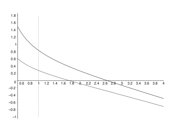
Figure 5: The values of the masses for D2

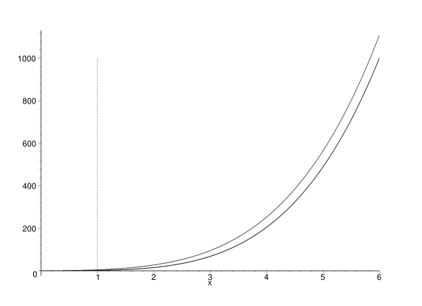
Figure 6: The values of the masses for D4

• Since, as discussed above, the geodesic line makes sense only for $z\geq{\mu\over E}$, apart from a small region where $\sqrt{13-3p\over 3-p}{\mu\over E}\geq z\geq{\mu\over E}$ for $m_{x}^{2}$ and $\sqrt{p+1\over 3-p}{\mu\over E}\geq z\geq{\mu\over E}$ for $m_{y}$, the masses–squared are negative as can be seen in figures 4–6.

One can check that these negative value of $m^{2}$ are consistent with the SUGRA equations of motions. As discussed above in section 2 the Ricci tensor is related to the masses as follows

$$R_{++}=(p+1)m_{x}^{2}+(7-p)m_{y}^{2}$$ (5.21)

Recall that one of the SUGRA equations of motion takes the form

$$R_{MN}=-2\nabla_{M}\nabla_{N}\phi+{1\over 96}e^{2\phi}[F_{M...}F_{N}^{...}-{1\over 10}G_{MN}F_{...}F^{...}]$$ (5.22)

where ${}_{...}\ ^{...}$ denotes contracted indices. Applying this to $R_{++}$ we have for our case

$$R_{++}=-2\partial_{+}\partial_{+}\phi+{1\over 96}e^{2\phi}[F_{+...}F_{+...}]$$ (5.23)

Had the dilaton been constant, this equation would imply that the sum $\sum m^{2}$ must be positive, however this is not the case here since we have a running dilaton. In fact it is easy to check that for large $z$ the dilaton term dominates the $F^{2}$ term so that one finds

$$R_{++}\rightarrow_{z\rightarrow\infty}-2{(7-p)(3-p)\over(5-p)^{2}}z^{-2{3-p\over 5-p}}E^{2}z^{2}$$ (5.24)

which is equal to the asymptotic value of $(p+1)m_{x}^{2}+(7-p)m_{y}^{2}$.

5.2 Comments on negative negative masses–squared

The issue of negative masses is a very interesting and intricate one and deserves a detailed study on its own. In general, pp-waves with negative masses make for a potentially very rich laboratory for exploring string theory in an expanding universe. Here we will attempt a much more modest heuristic approach and argue in favor of negative mass signaling a breakdown in the description for the quantum Hilbert space of asymptotic states.

First let us state that what we mean by negative mass originates from the coefficient $+\mu(x^{+})^{2}X_{i}^{2}(dx^{+})^{2}$ in the generic pp-wave metric in Brinkman coordinates. Note, first of all, that this term becomes a negative mass–squared for a worldsheet coordinate only after we take the light-cone gauge, that is $x^{+}=p^{+}\tau$. In other words, there is a gauge choice involved in this statement.

Another word of caution is in order: the tachyonic behavior is exclusively in the world sheet theory, that is, we are dealing with a tachyon in a $1+1$ dimensional field theory. From the spacetime point of view it does not make sense to define mass, as the system is not invariant under translation of $X^{i}$’s. The mass–squared term breaks this symmetry.

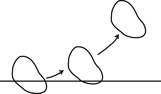
Figure 2: Motion of a stiff string in a background of negative mass squared.

PP-wave backgrounds with negative mass–squared appear very naturally in string theory [16]. In the absence of fluxes the Ricci tensor has to vanish and therefore there will be masses–squared of opposite signs. Based on the symmetries of these backgrounds it was argued in [16] that such backgrounds are exact string solutions to all orders in $\alpha^{\prime}$. Namely, the fact that only $R_{+i+j}$ is nonzero, combined with $g^{++}=0$, implies that all curvature tensors necessarily vanish. Such scalar tensors are precisely the $\alpha^{\prime}$ contribution to the SUGRA equations. However, Horowitz and Steif considered test strings and found that $<M^{2}>$ diverges, pointing to a quantum mechanical instability.

The clearest analogy (and the main intuition) for the motion of the string in these backgrounds is provided by a particle of energy $n^{2}$ moving in a potential given by $\mu(x^{+})^{2}$. The geodesic motion along the coordinates $X_{i}$ with negative mass is given by $\ddot{X}_{i}-\mu^{2}X_{i}=0$. This means that test masses will run away from the origin and feel a tidal force separating them of order $\mu^{2}$.

Coming back to string theory, we see that as long as the string tension $\alpha^{\prime}>\mu^{2}$, strings will behave like a classical particles and nothing unusual happens (see fig.2). Once $\mu^{2}>\alpha^{\prime}$, however, the string will be torn apart due to repulsive tidal forces. For any nonzero $g_{s}$, it will always be favorable for the string to split into smaller strings (see fig.3).

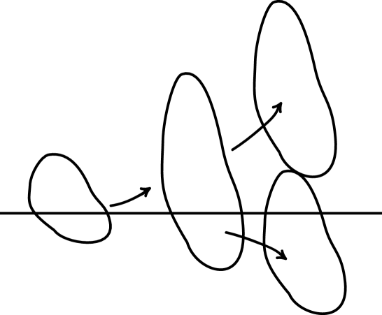
Figure 3: Motion and splitting of a string in a background of large negative mass squared.

This implies that the Hilbert space of asymptotic strings derived from the first-quantized string is no longer valid. Note that for highly excited strings $n^{2}>\mu^{2}$ these modes feel nothing.

In the rest of this section we describe possible ways to deal with the negative mass–squared issue in some of the D–p–brane solution. To do so we repeatedly use the D–p–brane maps described in [12] that point to the most appropriate theory to describe the degrees of freedom of a given Dp branes at different energy scale.

5.3 $p=1$ the flow from $D_{1}$ to $F_{1}$

Figure 4: The values of the masses for D1

In this case the solution can be written as

$$ds^{2}=-4dx^{+}dx^{-}+{3\over 16}z^{-1}\bigg{[}(E^{2}z^{2}-5\mu^{2})\sum\limits_{i=1}^{2}x_{i}^{2}+(E^{2}z^{2}-\mu^{2})\sum\limits_{j=3}^{8}x_{j}^{2}\bigg{]}(dx^{+})^{2}+\sum\limits_{i=1}^{8}dx_{i}^{2},$$ (5.25)

where $x^{+}=\left({2\over E\mu}\right)^{1/2}F(\sqrt{{Ez\over\mu}+1},{1\over\sqrt{2}})$ and $F()$ is a hyper–geometric function. As can be seen from figure 4 the masses of this solution are mostly negative and we naturally turn to the whole D1-map to understand this situation better.

The $D_{1}$ SUGRA background [12] can be trusted only in the ${1\over\sqrt{g^{2}_{Y}MN}}<<z<<{1\over\sqrt{g^{2}_{Y}MN}}N^{2/3}$ otherwise either the curvature or the string coupling are not small. For $z$ smaller then the lower bound one has to use the description of the $1+1$ SYM theory with 16 supersymmetries. In the IR side of the allowed window, where the dilaton becomes large, one performs an S-duality transformation and then describe the system as the near horizon limit of large $N$ fundamental strings. The Penrose limit of this background can be taken following the same lines as for the $D_{1}$ background. Had we taken the limit on the Einstein metric of the fundamental string, obviously the limit would be the same as the one of the $D_{1}$ string since the Einstein metric does not change under S-duality. However, the relevant metric here is obviously the string metric. For this metric the geodesic line $\partial_{x^{+}}z$ and the corresponding mass $m_{x}^{2}$ take the form

$$\partial_{x^{+}}z = \pm{z}^{2}\sqrt{z^{2}E_{F_{1}}^{2}-\mu_{F_{1}}^{2}}$$ (5.26)

$$m_{x}^{2} = {3/4}z^{2}\bigg{[}E_{F_{1}}^{2}z^{2}+\mu_{F_{1}}^{2}\bigg{]}$$ (5.27)

where the $E_{F_{1}}$ and $\mu_{F_{1}}^{2}$ are the corresponding integration constants. Recall that for the $D_{1}$ the geodesic and the mass are given by

$$\partial_{x^{+}}z = \pm\sqrt{z}\sqrt{z^{2}E_{D_{1}}^{2}-\mu_{D_{1}}^{2}}$$ (5.28)

$$m_{x}^{2} = 3/16z^{-1}\bigg{[}-E_{D_{1}}^{2}z^{2}+5\mu_{D_{1}}^{2}\bigg{]}$$ (5.29)

It is thus clear that in the IR region where the $D1$ description ceases to be valid, the squared masses become positive again. For given parameters $E_{D_{1}}$ and $\mu_{D_{1}}^{2}$ one can guarantee continuity in the masses by adjusting the parameters of the string background $E_{F_{1}}$ and $\mu_{F_{1}}^{2}$.

5.4 D2 to M2 Flow in 11-d

As is typical of nonconformal Dp branes a given supergravity solution is part of a greater phase diagram called the D2-map in [12]. Here we review that map since it is crucial for us to understand which description is valid at each energy scale. Taking the Maldacena limit amounts to decoupling the bulk from the theory on the D2 branes which turns out to be a U(N) super-Yang-Mills in 2+1 dimensions, with 16 supersymmetries. At a given energy scale, $U$, the dimensionless effective coupling of the gauge theory is $g^{2}_{eff}\sim g_{YM}^{2}N/U$ and, hence, perturbative super-Yang-Mills can be trusted in the UV region where $g_{eff}$ is small $g_{YM}^{2}N\ll U$. The type II supergravity description can be trusted when the curvature (5.4) in string units and the effective string coupling are small $g^{2}_{YM}N^{1/5}\ll U\ll g_{YM}^{2}N$. We see that a necessary condition is to have $N\gg 1$. In the region $g_{eff}\approx 1$ we have a transition between the perturbative super-Yang-Mills description and the supergravity description.

In the region $U<g_{YM}^{2}N^{1/5}$ the dilaton becomes large. In other words the local value of the radius of the eleventh dimension, $R_{11}(U)$, becomes larger than the Planck scale since $R_{11}=e^{2\phi/3}l_{p}$. Even though the string theory is becoming strongly coupled we will be able to trust the supergravity solution if the curvature is small enough in eleven dimensional Planck units.

The relation between the eleven dimensional metric and the ten dimensional type IIA string metric, dilaton and gauge field is

$$ds^{2}_{11}=e^{4\phi/3}(dx_{11}+A^{\mu}dx_{\mu})^{2}+e^{-2\phi/3}ds^{2}_{10},$$ (5.30)

which implies that the curvature in 11D Planck units is

$$l^{2}_{p}R\sim e^{2\phi/3}\frac{1}{g_{eff}}\sim\frac{1}{N^{1/3}}\left(\frac{g^{2}_{YM}}{U}\right)^{1/3}.$$ (5.31)

For large $N$, in the region $g_{YM}^{2}<U$, the curvature in 11D Planck units is small. In the region $U<g_{YM}^{2}$ we should use a different solution corresponding to M2-branes localized on the circle associated with the 11th dimension.

The curvature of $N$ M2-branes in the field theory limit is $l^{2}_{p}R\sim\frac{1}{N^{1/3}}$. Note that the curvature does not depend on $U$ since the theory is conformal in the IR limit. We conclude, therefore, that for large $N$ the supergravity description is valid in the region $U\ll g_{YM}^{2}N^{1/5}$.

The M2 brane solution is characterized by a harmonic function $H$ and is given by

$$ds^{2}_{11}=H^{-2/3}dx^{2}_{||}+H^{1/3}dx^{2}_{\perp}$$ (5.32)

and there is also a fourform field strength given in terms of $H$. When we take $H\sim N/x^{6}$ we have a solution where the M2 branes are localized in the eight transverse non-compact dimensions. If one of the dimensions is compact (let us say the 11th dimension) we can take $H\sim N/r^{5}$ where now $r$ denotes the radial distance in the seven transverse non-compact dimensions. This is the solution we get from uplifting $N$ D2’s. The appropriate solution to think of interpolating between uplifted D2 and M2 is the one in which we take the M2 branes to be localized in the compact dimension so that the harmonic function is

$$H=\sum_{n=-\infty}^{\infty}{2^{5}\pi^{2}Nl_{p}^{6}\over(r^{2}+(x_{11}-x_{11}^{0}+2\pi nR_{11})^{2})^{3}}$$ (5.33)

with $x_{11}\sim x_{11}+2\pi R_{11}$. For distances much larger than $R_{11}$ we can Poisson resum this expression to

$$l_{p}^{3}H={6\pi^{2}g_{YM}^{2}N\over U^{5}}+\sum_{m=1}^{\infty}Ne^{-mU/g_{YM}^{2}}\cos(mx_{11}^{0}/R_{11}){\cal O}(U^{-5}),$$ (5.34)

where we have used that $R_{11}=g^{2}_{YM}{\alpha^{\prime}}$. For $g_{YM}^{2}\ll U$ we can, therefore, use the uplifted solution to describe the physics while for smaller values of $U$ we should use (5.33). Note that for such small energy scales it becomes necessary to specify the expectation value of $\phi^{11}=g_{YM}^{2}x_{11}^{0}/R_{11}$ which is the new scalar coming from dualizing the vector in 2+1 dimensions. For very low energies

$$U\ll g_{YM}^{2},$$ (5.35)

we are very close to the M2 branes and we can neglect the “images” in (5.33). Thus, the solution will resemble that of M2 branes in non-compact space and we have the conformal field theory with SO(8) symmetry.

The effective Lagrangian describing the motion along null geodesics for a metric of the form (5.32) is

$${\cal L}=-H^{-2/3}\dot{t}^{2}+H^{1/3}\dot{r}^{2}+H^{1/3}r^{2}\dot{\psi}^{2}.$$ (5.36)

The corresponding equations of motion

$$\dot{\psi}=\mu\,H^{-1/3},\qquad\dot{t}=E\,H^{2/3},\quad\dot{r}^{2}+{\mu^{2}\over H^{2/3}r^{2}}=E^{2}H^{1/3}.$$ (5.37)

The coordinate transformation that allows to perform the Penrose-Güven limit limit is,

$$r=r(u),\qquad t=t_{u}-{v\over E}+\mu\,\phi,\qquad\psi=\psi_{u}+E\,\phi,$$ (5.38)

where the subindex $u$ means that the corresponding term is a function of only $u$. After the Penrose limit the metric in Rosen coordinates takes the following form

$$ds^{2}=2dudv+(E^{2}\,H^{1/3}-\mu^{2}H^{-2/3})d\phi^{2}+H^{-2/3}(dx_{1}^{2}+dx_{2}^{2})+H^{1/3}\big{[}r^{2}\sin^{2}\psi_{u}ds^{2}({\bf R}^{5})+R_{11}^{2}dz^{2}\big{]}.$$ (5.39)

In the more familiar Brinkman coordinates

$$ds^{2} = -4dx^{+}dx^{-}-\big{[}\mu_{\phi}^{2}\phi^{2}+\mu^{2}_{p}(x_{1}^{2}+x_{2}^{2})+\mu^{2}_{y}(\sum\limits_{i=1}^{5}y_{i}^{2})+\mu^{2}_{z}z^{2}\big{]}(dx^{+})^{2}$$

$$+ d\phi^{2}+\sum\limits_{i=1}^{2}dx_{i}^{2}+\sum\limits_{i=1}^{5}dy_{i}^{2}+dz^{2},$$

$$\mu^{2}_{p} = {\mu^{2}\over 3\,r}\sqrt{{E^{2}r^{2}H\over\mu^{2}}-1}{d\over dr}\left({H^{\prime}\over H^{5/3}\,r}\sqrt{{E^{2}r^{2}H\over\mu^{2}}-1}\right),$$

$$\mu_{y}^{2} = {\mu^{2}\over H^{2/3}r^{4}}-{\mu^{2}\over H^{1/2}\,r^{2}}\sqrt{{E^{2}r^{2}H\over\mu^{2}}-1}{d\over dr}\left({(H^{1/6}r)^{\prime}\over H^{1/3}\,r}\sqrt{{E^{2}r^{2}H\over\mu^{2}}-1}\right).$$ (5.40)

The above solution is not very illuminating. For our purpose the most important information is contained in the limits. In the M2 limit $(N/r^{6})$ we naturally recover the expected result $\mu_{p}^{2}=4\mu^{2},\,\,\mu_{y}^{2}=\mu^{2}$. In the uplifted D2 limit

$$\mu^{2}_{p} = {20\mu^{2}\over L^{10/3}\,r^{2/3}}+{5\,E^{2}\,L^{5/3}\over 18\,r^{11/3}},$$

$$\mu^{2}_{y} = {35\mu^{2}\over 36\,L^{10/3}\,r^{2/3}}+{E^{2}\,L^{5/3}\over 9\,r^{11/3}},$$ (5.41)

The key observation we want to make is that the masses are nowhere negative.This result shows that once lifted to M-theory the possible instability is gone.

5.5 $p=4$

The behavior of Dp branes for $p>3$ is, as explained before, very different. In this subsection we discuss the D4.

In this particular case we are able to provide a closed-form solution for the Penrose-Güven limit . The metric is

$$ds^{2}=-4dx^{+}dx^{-}-{3\mu^{4}\over 4(E^{2}-\mu^{4}x_{+}^{2})^{2}}\bigg{[}(2E^{2}-\mu^{4}x_{+}^{2})\sum\limits_{i=1}^{5}x_{i}^{2}+(6E^{2}-\mu^{4}x_{+}^{2})\sum\limits_{j=6}^{8}x_{j}^{2}\bigg{]}(dx^{+})^{2}+\sum\limits_{i=1}^{8}dx_{i}^{2},$$ (5.42)

where $0\leq x_{+}\leq{E\over\mu^{2}}$.

6 Summary and discussion

An important goal of the gauge/string duality is to develop a dual picture of QCD. Since this is a formidable task, much simpler systems that include supersymmetry and conformal invariance were analyzed first. At a later stage the duality associated with non-conformal gauge theories was also addressed[10]. The corresponding RG flows were mapped into the evolution of certain SUGRA modes. It the present work an attempt has been made to go a step forward by mapping the RG flows into an evolution on the world sheet of the string model derived using the Penrose[2] limit. In fact we argued that an essential part of the flow is captured by a QM particle theory on the tdppw background. In this language the system is mapped into a harmonic oscillator with time dependent frequency. We use the tool kit that has been developed to solve this well known QM problem to gain insight on the operator mixing of the gauge theory. The main point that we have made in this regard is that the QM associated with the tdppw limit is exactly solvable.

We then demonstrated these ideas by explicitly constructing the Penrose limit of the PW solution. We showed that in the IR fixed point one can take two null geodesics. The associated gauge theory flows were analyzed. It is remarkable that the killing vectors deduced from the limit on the geometry side were mapped into global currents of the gauge theory that led to a simple structure of the gauge theory operators duals of the low lying string states.

Another class of models that we have analyzed is that of the near horizon limit of the large number of $D_{p}$ branes[12]. We wrote the equations of the null geodesic lines and the masses of the string model. It turns out that for $p<3$ the masses–squared become very negative, namely there is a large upside–down potential unbounded from below. This signals that the world sheet theory has become inadequate, and points to the necessity for a different description of the IR region. In the SUGRA picture this was caused by large string coupling or large curvature.

The work on this paper has raise several related open questions that are under current investigation. Here is a short list of them: (i) We have made only a very limited use of the knowledge about the QM system. A natural question to ask is how to map all the properties of this system to those of the dual gauge theory. In particular one can construct special states like coherent and squeezed states. It is not clear to what do these state translate in the gauge theory operators language. (ii) For what tdppw string models can one provide an exact solution similar to the exact solution of the QM problem. (iii) The Penrose limit at any generic point along the (PW) flow and not only at the fixed points, with a better understanding for the roles of the 3–forms. (iv) The study of tdppw of SUGRA space-times that are duals to confining gauge theories. (v) The precise map of the CS equation in the tdppw string picture.

Acknowledgments

We have benefited from discussions with D. Berenstein, T. Brun, M. Einhorn, A.Hashimoto, F. Larsen J. Maldacena, H. Nastase, S. Sethi, M. Strassler, C. Thorn and D. Vaman. We are specially grateful to J. Maldacena for a careful reading of the manuscript and useful discussions and to N. Seiberg for several illuminating conversations.

Appendix A Penrose limit of a general metric

In this appendix we provide the Penrose-Güven limit for the Pilch-Warner background for an arbitrary value or $r$. The purpose is to outline how we can, in principle, trace a particular geodesic throughout the flow, that is, for values of $r$ in both the IR and UV regions. Since the Pilch-Warner solution is not known analytically for any value of the $r$ our calculation is limited to the regions where the solution is known. However, it allows us to understand better the general scheme of Penrose limits in the presence of RG flows.

We will divide the problem into two stages. The first one is general and we apply its results throughout the paper. Consider a metric of the form:

$$ds^{2}=-g_{tt}dt^{2}+g_{rr}^{2}dr^{2}+g_{\psi\psi}^{2}d\psi^{2}+g_{ij}dY^{i}dY^{j},$$ (A.1)

where $g_{ij}(r)$, that is, is the metric is a function of $r$ only. The effective Lagrangian for the null geodesic is

$${\cal L}=-g_{tt}(r)\dot{t}^{2}+g_{rr}(r)\dot{r}^{2}+g_{\psi\psi}(r)\dot{\psi}^{2},$$ (A.2)

where dots represent derivatives with respect to the affine parameter $U$. Since the effective Lagrangian is explicitly independent of $t$ and $\psi$ we have the following equations of motion

$$\dot{t} = {E\over g_{tt}},\qquad\dot{\psi}={\mu\over g_{\psi\psi}},$$

$$\dot{r}^{2} = {E^{2}\over g_{rr}g_{tt}}-{\mu^{2}\over g_{rr}g_{\psi\psi}}$$ (A.3)

Introducing new coordinates $(U,V,\Phi)$ such that

$$r=r_{U},\quad t=t_{U}-{v\over E}+\mu\phi,\quad\psi=\psi_{U}+E\Phi,$$ (A.4)

where $x^{i}_{U}$, a function of $U$ only, is determined by (Appendix A Penrose limit of a general metric ) we guarantee that $g_{UU}=g_{U\Phi}=0$ and $g_{UV}=1$. The new metric becomes

$$ds^{2}=2dUdV-{1\over E^{2}}g_{tt}dV^{2}+{2\mu\over E}g_{tt}dVd\Phi+(E^{2}g_{\psi\psi}-\mu^{2}g_{tt})d\Phi^{2}+g_{ij}dY^{i}dY^{j}.$$ (A.5)

Taking the Penrose limit means

$$ds^{2} = \Omega^{-2}ds^{2}(\Omega),$$

$$U = u,\quad V=\Omega^{2}v,\quad\Phi=\Omega\phi,\quad Y^{i}=\Omega y^{i},$$

$$\Omega \to 0.$$ (A.6)

The resulting metric is

$$ds^{2}=2dudv+(E^{2}g_{\psi\psi}-\mu^{2}g_{tt})d\phi^{2}+g_{ij}dy^{i}dy^{j},$$ (A.7)

where the metric entries, $g_{\alpha\beta}$, are only a function of $u$. This metric can be taken to Brinkman coordinates. In particular, the mass associated $\phi$ will be

$$m_{\phi}^{2}=-{\big{[}\sqrt{E^{2}g_{\psi\psi}-\mu^{2}g_{tt}}\big{]}^{\prime\prime}\over\sqrt{E^{2}g_{\psi\psi}-\mu^{2}g_{tt}}},$$ (A.8)

where the prime means derivatives with respect to $x^{+}=u$. For a diagonal $g_{ij}$ the mass associated with the coordinate $x_{i}$ is

$$m_{i}^{2}=-{(\sqrt{g_{ii}})^{\prime\prime}\over\sqrt{g_{ii}}}.$$ (A.9)

We now turn to the Pilch-Warner solution which can be written as:

$$ds_{10}^{2} = \Omega^{2}\left(e^{2A}\big{[}-dt^{2}+dx_{1}^{2}+dx_{2}^{2}+dx_{3}^{2}\big{]}+dr^{2}\right)+ds_{5}^{2},$$

$$ds_{5}^{2} = g_{\theta\theta}d\theta^{2}+g_{\theta_{1}\theta_{1}}d\theta_{1}^{2}+g_{\phi\phi}d\phi^{2}+g_{\phi_{1}\phi_{1}}d\phi_{1}^{2}+g_{\psi_{1}\psi_{1}}d\psi_{1}^{2}$$ (A.10)

$$+ 2g_{\phi\phi_{1}}d\phi d\phi_{1}+2g_{\phi\psi_{1}}d\phi d\psi_{1}+2g_{\phi_{1}\psi_{1}}d\phi_{1}d\psi_{1}.$$

where

$$g_{\theta\theta} = {L^{2}\,\Omega^{2}\over{\bar{\rho}}^{2}\,\cosh^{2}\chi},$$

$$g_{\theta_{1}\theta_{1}} = {L^{2}\,\Omega^{2}\,{\bar{\rho}}^{4}\cos^{2}\theta\over 4\,\bar{X}_{1}\,\cosh^{2}\chi},$$

$$g_{\phi\phi} = {L^{2}\,\Omega^{2}\,\bar{X}_{2}\,\sin^{2}\theta\over{\bar{\rho}}^{2}\,\cosh\chi\,\bar{X}_{1}^{2}},$$

$$g_{\phi_{1}\phi_{1}} = {L^{2}\,\Omega^{2}\over{\bar{\rho}}^{2}\,\cosh^{2}\chi}\bigg{[}{{\bar{\rho}}^{6}\,\cosh\chi\,\cos^{2}\theta\over 4\bar{X}_{2}}+{{\bar{\rho}}^{12}\sinh^{4}\chi\cos^{4}\theta\sin^{2}\theta\over 4\bar{X}_{1}^{2}\bar{X}_{2}\cosh\chi}\bigg{]},$$

$$g_{\psi_{1}\psi_{1}} = {L^{2}\,\Omega^{2}\over{\bar{\rho}}^{2}\,\cosh^{2}\chi}\bigg{[}{{\bar{\rho}}^{6}\,\cosh\chi\,\cos^{2}\theta\,\cos^{2}\theta_{1}\over 4\bar{X}_{2}}+{{\bar{\rho}}^{12}\sinh^{4}\chi\cos^{4}\theta\sin^{2}\theta\cos^{2}\theta_{1}\over 4\bar{X}_{1}^{2}\bar{X}_{2}\cosh\chi}+{{\bar{\rho}}^{6}\cos^{2}\theta\sin^{2}\theta_{1}\over 4\bar{X}_{1}}\bigg{]},$$

$$g_{\phi\phi_{1}} = {L^{2}\,\Omega^{2}\,{\bar{\rho}}^{4}\,\sinh^{2}\chi\,\cos^{2}\theta\,\sin^{2}\theta\over\bar{X}_{1}^{2}\cosh^{2}\chi},$$

$$g_{\phi\psi_{1}} = {L^{2}\,\Omega^{2}\,{\bar{\rho}}^{4}\,\sinh^{2}\chi\,\cos^{2}\theta\,\sin^{2}\theta\,\cos\theta_{1}\over\bar{X}_{1}^{2}\cosh^{2}\chi},$$

$$g_{\phi_{1}\psi_{1}} = {L^{2}\,\Omega^{2}\,{\bar{\rho}}^{4}\,\cos^{2}\theta\,\cos\theta_{1}\over 4\bar{X}_{2}\,\cosh^{2}\chi}\bigg{[}\cosh\chi+{{\bar{\rho}}^{6}\sinh^{4}\chi\cos^{2}\theta\sin^{2}\theta\over\bar{X}_{1}^{2}\cosh\chi}\bigg{]}.$$ (A.11)

The complex 3–form ${\cal A}_{(2)}$ is:

$${\cal A}_{(2)}=e^{-i(\phi+\phi_{1})}\,{L^{2}\over 8}\bigg{[}i\cos\theta\ d\theta-{\cos^{2}\theta\sin\theta\over 1+\sin^{2}\theta}(d\phi+\cos\theta_{1}\ d\psi-d\psi)\bigg{]}\wedge(d\theta_{1}\ +i\sin\theta_{1}\ d\psi_{1})$$ (A.12)

Note that in general $g_{ij}(r,\theta,\theta_{1})$. Following the general approach we would like to find coordinates in which the above metric takes the form:

$$ds^{2}=d\beta(d\lambda+ad\beta+b_{i}dY^{i})+C_{ij}dY^{i}dY^{j},$$ (A.13)

where $a,b_{i}$ and $C_{ij}$ can depend on any coordinate. This task involve considering a geodesic for which, in principle, all functions will depend nontrivially on the affine parameter. One is therefore, to consider an effective Lagrangian of the form:

$${\cal L}=-g_{tt}\dot{t}^{2}+g_{rr}\dot{r}^{2}+g_{\theta\theta}\dot{\theta}^{2}+g_{\theta_{1}\theta_{1}}\dot{\theta}_{1}^{2}+g_{ij}\dot{x}_{i}\dot{x}_{j},$$ (A.14)

where $x_{i}=\{\phi,\phi_{1},\psi_{1}\}$. Since the metric does not explicitly depends on $x_{i}$ we will have three integrals of motion that reduce the equations of motion for $x_{i}$ to first order differential equations. We are thus left with three second order differential equations for $\{r,\theta,\theta_{1}\}$, one of which can be exchanged by a first order equation which is the condition of the geodesic being null: ${\cal L}=0$. With similar coordinate transformations to those described in the main body we bring the metric to the required form and subsequently perform the Penrose limit.

A different approach that exploits the symmetry of the problem is to used the procedure outlined above, supplemented by the approach used by BMN which makes use of the specific form of the metric. In the BMN approach the metric automatically takes the Brinkman form. Namely, we will expand around a particular value of $\theta$ and $\theta_{1}$, at this point it does not matter which particular value. In the main body we naturally considered, for example, $\theta=\pi/2$ and $\theta=0$. The nature of the dependence of $g_{ij}(r,\theta,\theta_{1})$ on $\theta$ and $\theta_{1}$ is such that we obtain $g_{ij}(r,\theta,\theta_{1})=g_{ij}(r)\big{[}1+a(r){y^{2}\over L^{2}}+b(r){x^{2}\over L^{2}}\big{]}+{\cal O}(L^{-3})$. We have, by means of expanding in $\theta$ and $\theta_{1}$, reduced the problem to the one considered at the beginning of the appendix. We can now consider a geodesic that is determined motion in $(t,r,\vartheta)$ where $\vartheta$ is one of the angles of $S^{5}$ or a combination of them. The only difference being that in addition to the standard contribution to $g_{++}$ discussed in the first part of the appendix due to going from Rosen to Brinkman coordinates, we now have a contribution due to the expansion discussed above.

Although conceptually less straightforward the described method to the Penrose limit is very efficient technically. In the case of $AdS_{5}\times S^{5}:-\cosh^{2}\rho dt^{2}+d\rho^{2}+\sinh^{2}\rho d\Omega_{3}^{2}+d\theta^{2}+\cos^{2}\ d\psi^{2}+\sin^{2}\theta\tilde{\Omega}_{3}^{2}$ it is especially simple, expanding around $\rho=r/L$ and $\theta=y/L$

$$L^{-2}\,ds_{AdS_{5}}^{2} = -(1+{r^{2}\over L^{2}}+{\cal O}(L^{-4}))dt^{2}+{dr^{2}\over L^{2}}+({r^{2}\over L^{2}}+{\cal O}(L^{-4}))d\Omega_{3}^{2},$$

$$L^{-2}\,ds_{S^{5}}^{2} = (1-{y^{2}\over L^{2}}+{\cal O}(L^{-4}))d\psi^{2}+{dy^{2}\over L^{2}}+({y^{2}\over L^{2}}+{\cal O}(L^{-4}))d\tilde{\Omega}_{3}^{2}.$$ (A.15)

The effective Lagrangian analogous to the one considered in the previous appendix is now

$${\cal L}=-\dot{t}^{2}+\dot{\psi}^{2},$$ (A.16)

making the whole task straightforward. There is one last detail in taking the Penrose limit that has very important physical implications. In the case of the Pilch-Warner background the metric is not diagonal. Similar to the case of the $AdS_{5}\times T^{1,1}$ one needs to shift some of the coordinates by a function of $x^{+}$. Without shifting we have that following (A.2) and (Appendix A Penrose limit of a general metric )

$${\partial\over\partial x^{+}}=\dot{t}\partial_{t}+\dot{r}\partial_{r}+\dot{\psi}\partial_{\psi}.$$ (A.17)

However, it will generically be the case that the metric contains some nondiagonal terms of the form $l(x^{+})dx^{+}d\vartheta$. We can cancel those terms by simply shifting $\vartheta\to\vartheta+f(x^{+})$, such that

$$l(x^{+})dx^{+}d\vartheta+p(x^{+})d\vartheta d\vartheta\to p(x^{+})d\vartheta d\vartheta-{l^{2}\over 4p}(dx^{+})^{2}$$ (A.18)

This shift changes the masses of some of the field and more importantly changes the definition of $P^{-}$ since now

$${\partial\over\partial x^{+}}=\dot{t}\partial_{t}+\dot{r}\partial_{r}+\dot{\psi}\partial_{\psi}-{l\over 2p}\partial_{\vartheta}.$$ (A.19)

It might not always be possible to diagonalize the coefficient of $g_{++}$ which in general is of the form $A_{ij}(x^{+})x^{i}x^{j}$, in particular we have implicitly used the fact that both terms of (A.18) are multiplied by an overall function of say $y^{2}$ or $x^{2}$. In case the terms in (A.18) are multiplied by different powers of $y$ or $x$ we can not diagonalize the metric in this and will, in general, have “magnetic” terms.

References

• [1] J. Maldacena, “The large N limit of superconformal field theories and supergravity,” Adv. Theor. Math. Phys.  2 (1998) 231[hep-th/9711200].
S.S. Gubser, I.R. Klebanov and A.M. Polyakov, “Gauge theory correlators from non-critical string theory,” Phys. Lett. B428 (1998) 105 [hep-th/9802109].
E. Witten, “Anti-de Sitter space and holography,” Adv. Theor. Math. Phys.  2 (1998) 253 [hep-th/9802150].
• [2] R. Penrose, “Any space-time has a plane wave as a limit”, in Differential Geometry and Relativity, Reidel, Dordrecht, 1976.
R. Penrose, “Techniques of Differential Topology in Relativity”, SIAM,1972.
• [3] R. Güven, “Plane wave limits and T-duality,” Phys. Lett. B 482 (2000) 255 [arXiv:hep-th/0005061].
• [4] M. Blau, J. Figueroa-O’Farrill and G. Papadopoulos, “Penrose limits, supergravity and brane dynamics,” arXiv:hep-th/0202111.
• [5] M. Blau, J. Figueroa-O’Farrill, C. Hull and G. Papadopoulos, “Penrose limits and maximal supersymmetry,” arXiv:hep-th/0201081.
M. Blau, J. Figueroa-O’Farrill, C. Hull and G. Papadopoulos, “A new maximally supersymmetric background of IIB superstring theory,” JHEP 0201 (2002) 047 [arXiv:hep-th/0110242].
• [6] D. Berenstein, J. Maldacena and H. Nastase, “Strings in flat space and pp waves from N = 4 super Yang Mills,” arXiv:hep-th/0202021.
• [7] R. R. Metsaev, “Type IIB Green-Schwarz superstring in plane wave Ramond-Ramond background,” Nucl. Phys. B 625 (2002) 70 [arXiv:hep-th/0112044].
• [8] R. R. Metsaev and A. A. Tseytlin, “Exactly solvable model of superstring in plane wave Ramond-Ramond background,” arXiv:hep-th/0202109.
• [9] D. Z. Freedman, S. S. Gubser, K. Pilch and N. P. Warner, “Renormalization group flows from holography supersymmetry and a c-theorem,” Adv. Theor. Math. Phys.  3 (1999) 363 [arXiv:hep-th/9904017].
• [10] K. Pilch and N. P. Warner, “N = 1 supersymmetric renormalization group flows from IIB supergravity,” Adv. Theor. Math. Phys.  4 (2002) 627 [arXiv:hep-th/0006066].
• [11] R. G. Leigh and M. J. Strassler, “Exactly marginal operators and duality in f our-dimensional N=1 supersymmetric gauge theory,” Nucl. Phys. B 447 (1995) 95 [arXiv:hep-th/9503121].
• [12] N. Itzhaki, J. M. Maldacena, J. Sonnenschein and S. Yankielowicz, “Supergravity and the large N limit of theories with sixteen supercharges,” Phys. Rev. D 58 (1998) 046004 [arXiv:hep-th/9802042].
• [13] L. A. Pando Zayas and J. Sonnenschein, “On Penrose limits and gauge theories,” JHEP 0205 (2002) 010 [arXiv:hep-th/0202186].
• [14] H. J. Boonstra, K. Skenderis and P. K. Townsend, “The domain wall/QFT correspondence,” JHEP 9901 (1999) 003 [arXiv:hep-th/9807137].
• [15] O. Aharony, S. S. Gubser, J. Maldacena, H. Ooguri and Y. Oz, “Large N field theories, string theory and gravity,” Phys. Rept.  323 (2000) 183 [arXiv:hep-th/9905111].
• [16] G. T. Horowitz and A. R. Steif, “Space-Time Singularities In String Theory,” Phys. Rev. Lett.  64 (1990) 260.
G. T. Horowitz and A. R. Steif, “Strings In Strong Gravitational Fields,” Phys. Rev. D 42 (1990) 1950.
• [17] For instance see S. P. Kim and C. H. Lee, “Nonequilibrium quantum dynamics of second order phase transitions,” Phys. Rev. D 62, 125020 (2000), and reference therein.
• [18] D.C. Khandekar and S.V. Lawande “Exact propagator for time dependent harmonic oscillator with and without a singular perturbation” Jour. of Mtah Phys. 16 2 (1975) 384
• [19] H. R. Lewis, Jr and W. B¿ Riesenfeld 11 An exact Quantum theory of time-dependent Harmonic oscillator and of a charged particle in a time-dependent Electromagnetic field” Jour. of Mtah Phys. 10 8 (1969) 1458
• [20] U. Gursoy, C. Nunez and M. Schvellinger, “RG flows from Spin(7), CY 4-fold and HK manifolds to AdS, Penrose limits and pp waves,” arXiv:hep-th/0203124.
S. R. Das, C. Gomez and S. J. Rey, “Penrose limit, spontaneous symmetry breaking and holography in pp-wave background,” arXiv:hep-th/0203164.
D. Berenstein and H. Nastase, “On lightcone string field theory from super Yang-Mills and holography,” arXiv:hep-th/0205048.
V. E. Hubeny, M. Rangamani and E. Verlinde, “Penrose limits and non-local theories,” arXiv:hep-th/0205258.
• [21] R. Corrado, N. Halmagyi, K. D. Kennaway and N. P. Warner, “Penrose Limits of RG Fixed Points and PP-Waves with Background Fluxes,” arXiv:hep-th/0205314.
• [22] J. Sonnenschein, RG flows and strings on pp–wave background, talk presented at Mathematics and Physics of Extra Dimensions, Ann Arbor Michiga, April, 2002. and DPF Meeting Williamsburg, May 2002.
• [23] C. V. Johnson, K. J. Lovis and D. C. Page, “The Kaehler structure of supersymmetric holographic RG flows,” JHEP 0110, 014 (2001) [arXiv:hep-th/0107261]. “Probing some N = 1 AdS/CFT RG flows,” JHEP 0105 (2001) 036 [arXiv:hep-th/0011166].
• [24] K. Pilch and N. P. Warner, “A new supersymmetric compactification of chiral IIB supergravity,” Phys. Lett. B 487, 22 (2000) [arXiv:hep-th/0002192].