Domain walls in three-field models

Abstract

We investigate the presence of domain walls in models described by three real scalar fields. We search for stable defect structures which minimize the energy of the static field configurations. We work out explict orbits in field space and find several analytical solutions in all BPS sectors, some of them presenting internal structure such as the appearence of defects inside defects. We point out explicit applications in high energy physics, and in other branches of nonlinear science.

This paper deals with domain walls presenting internal structure that may engender nontrivial phenomena. Specifically we propose new systems of three coupled real scalar fields whose dynamics are controlled by superpotentials in the bosonic sector of supersymmetric theories. The systems allow for a multiplicity of solitonic solutions including the presence of defects inside defects, introducing new results that lead to a variety of applications in diverse fields of physics, chemistry and biology.

Domain walls may involve energy scales as different as those found in fields of magnetic systems ms , nonequilibrium thermodynamics wal and cosmology co . Usually, domain walls are immersions in $(3,1)$ dimensions of linear kink-like defects living in $(1,1)$ dimensions. These extended spatial structures are the basic building blocks to describe the coexistence of different domains or phases, and they are usually modeled by a set of scalar fields playing the role of order parameters satisfying amplitude equations. They also appear in models that include supersymmetry susy1 ; susy2 ; susy3 ; susy4 and supergravity sugra1 ; sugra2 . In particular, a great deal of attention has been given to the restrictions imposed by supersymmetry in the classification and solution of the solitonic field equations – in a supersymmetric theory one can categorize the topological defects as BPS and non-BPS states, according to the work of Bogomol’nyi and of Prasad and Sommerfield bps .

In models described by a single real scalar field we may distinguish at least two classes of systems, one that supports a single type of defect, and the other, that supports two or more different defects. We exemplify this by recalling the $\phi^{4}$ model, which supports a single type of defect, the tanh-like kink, and the double sine-Gordon model, which may support two different defects, the large and the small kinks 01 . On the other hand, models containing two or more real scalar fields give rise to at least two other classes of systems - those that support defects that engender internal structure is1 ; is2 and, those that support junctions of defects susy1 ; susy3 ; susy4 . In the latter context, in Ref. 00 , one has investigated the possibility of a regular hexagonal network of defects to spring in a model described by two real scalar fields. In Ref. 00a the idea of an hexagonal network of defect to be nested inside a topological defect has been investigated in a model described by three real scalar fields. That investigation has shown that when the host domain wall is driven to relax to cylindrical or spherical shape, the nested hexagonal network could give rise to structures resembling nanotubes or fulerenes, respectively. Similar ideas have been recently presented in bb , in the case of a soliton star that entraps a fulerenelike network of domain walls, and in bs , where the Skirme model is used to show the presence of fulerenelike structures in light nuclei, and also in ff , in the case of solutions of the Einstein equations describing black holes pierced by cosmic strings, forming structures that very much resemble the Platonic solids.

In Refs.00 ; 00a one has given up supersymmetry, to circumvent issues concerning stability of the nested network of domain walls. Here, however, we return to the basic problem, which concerns investigating models described by three real scalar fields in the bosonic portion of supersymmetric theories. Models with three real scalar fields have been studied before, for instance in an $O(3)$ model which admits unstable embedded walls ab , and also in agg , which investigates stability of kinks in a deformed $O(3)$ linear sigma model. Other motivations include the possibility of building spatial junctions of defects, instead of the planar junctions considered in susy3 ; susy4 , and the issue of finding a host domain wall that entraps a network of defects within the framework of supersymmetry. To construct spatial junctions of defects one first recalls the simpler issue, of contructing planar junctions. As we know, we can tile the plane with regular polygons in three distinct ways: with triangles, squares or hexagons. These cases require junctions with six, four and three legs, respectively. Thus, the two-field model should engender discrete $Z_{6}$, $Z_{4}$, or $Z_{3}$ symmetry. Interestingly, however, we notice that the triangular lattice is dual to the hexagonal lattice, and vice versa, and that the squared lattice is self-dual. This means that there is a dual relation between the (triangular, square or hexagonal) disposition of minima in the two-field model, and the (hexagonal, square or triangular) lattice made with the junction that spring with the very same minima. We take this as a guide to construct spatial junctions of defects in three-field models, to fill space with regular polyhedra. Before investigating such issue, however, let us first deal with the more general problem of finding topological defects in three-field models engendering discrete symmetry.

In general we are interested in potentials that can be obtained in terms of superpotentials, in the form

$$V=\frac{1}{2}W^{2}_{\phi}+\frac{1}{2}W^{2}_{\chi}+\frac{1}{2}W^{2}_{\rho}$$ (1)

where $W_{\phi_{i}}=\partial W/\partial\phi_{i}$, $\phi_{i}=\phi,\chi,\rho$. The energy density for static solutions that depend on the single spatial coordinate $x$ can be written as

$${\cal E}(x)=\frac{dW}{dx}+\sum_{i}\left(\frac{d\phi_{i}}{dx}-W_{\phi_{i}}\right)^{2}$$ (2)

It can be minimized to give $E_{ab}=|\Delta W_{ab}|$, with

$$\Delta W_{ab}=W_{a}-W_{b}$$ (3)

where the indices identify vacuum states, such that $W_{a}=W({\bar{\phi}}_{a},{\bar{\chi}}_{a},{\bar{\rho}}_{a})$ and so forth. This energy is the energy of Bogomol’nyi-Prasad-Sommerfield (BPS) solutions bps ; b1 . The BPS states obey the first order ordinary differential equations

$$\frac{d\phi}{dx}=W_{\phi},\;\;\;\;\;\frac{d\chi}{dx}=W_{\chi},\;\;\;\;\;\frac{d\rho}{dx}=W_{\rho}$$ (4)

We now introduce the model, given by the superpotential depending on two real parameters, $r$ and $s$,

$$W=\phi-\frac{1}{3}\phi^{3}-r\phi(\chi^{2}+\rho^{2})+rs\rho^{2}$$ (5)

Here we are using dimensionless space-time coordinates and fields. The corresponding potential is

$$V = \frac{1}{2}(1-\phi^{2})^{2}+2r^{2}\phi^{2}\chi^{2}+\frac{1}{2}r^{2}(\chi^{2}+\rho^{2})^{2}+$$ (6)

$$-r(1-\phi^{2})(\chi^{2}+\rho^{2})+2r^{2}(\phi-s)^{2}\rho^{2}$$

It may support two, four, and six minima, depending on the values of the two real parameters $r\neq 0$ and $s\neq 0$. In the case of six minima, for $r>0$ and $-1<s<1$ we get

$$v_{1,2} = \left(\pm 1,0,0\right)$$ (7)

$$v_{3,4} = \left(0,\pm\sqrt{\frac{1}{r}},0\right)$$ (8)

$$v_{5,6} = \left(s,0,\mp\sqrt{\frac{1}{r}(1-s^{2})}\;\right)$$ (9)

The model engenders the $Z_{2}\times Z_{2}$ symmetry, corresponding to reflections in the $\chi$ and $\rho$ axes. The presence of the $s$-dependent term in the superpotential forbids reflection symmetry in the $\phi$ axis. However, we notice that the operation $\phi\to-\phi$ leads the system to a partner system, in which one changes $s\to-s$.

Before studying the topological solutions of this system, it is interesting to analyse the projections over diverse axis and planes. The projection of the potential over the $\phi$ axis gives

$$V(\phi,0,0)=\frac{1}{2}(1-\phi^{2})^{2}$$ (10)

which is known to produce kink-like domain walls that may host internal structure. In the $(\phi,\chi)$ plane we have

$$V(\phi,\chi,0) = \frac{1}{2}(1-\phi^{2})^{2}+2r^{2}\phi^{2}\chi^{2}$$ (11)

$$-r(1-\phi^{2})\chi^{2}+\frac{1}{2}r^{2}\chi^{4}$$

We see that inside the domain wall

$$V(0,\chi,0)=\frac{1}{2}r^{2}\left(\frac{1}{r}-\chi^{2}\right)^{2}$$ (12)

and that outside the wall

$$V(\pm 1,\chi,0)=2r^{2}\chi^{2}+\frac{1}{2}r^{2}\chi^{4}$$ (13)

Thus, if the $\phi$ field gives rise to a domain wall, then inside this wall the $\chi$ field generates another defect. Notice that the squared masses of the $\chi$ field inside and outside of the domain wall are given by $m^{2}_{\chi}(in)=4r$ and $m^{2}_{\chi}(out)=4r^{2}$, showing that the parameter $r$ may be used to control the presence of elementary $\chi$ mesons inside or outside the host domain wall, according to $r$ being greater or smaller than unit, respectively.

The projection of the potential in the $(\phi,\rho)$ plane gives

$$V(\phi,0,\rho) = \frac{1}{2}(1-\phi^{2})^{2}+2r^{2}(\phi-s)^{2}\rho^{2}$$ (14)

$$-r(1-\phi^{2})\rho^{2}+\frac{1}{2}r^{2}\rho^{4}$$

which takes the following forms, inside and outside the wall

$$V(0,0,\rho)=\frac{1}{2}+r(2rs^{2}-1)\rho^{2}+\frac{1}{2}r^{2}\rho^{4}$$ (15)

$$V(\pm 1,0,\rho)=2r^{2}(1\mp s)^{2}\rho^{2}+\frac{1}{2}r^{2}\rho^{4}$$ (16)

Clearly there is no spontaneous symmetry breaking (SSB) outside the host domain wall, but for $2rs^{2}<1$ there is SSB inside the host domain wall and the system may generate domain walls with internal structure. The mass of the $\rho$ meson inside the host wall, in this case, reads $m^{2}_{\rho}(in)=4r(1-2rs^{2})$. Outside the host wall there is an asymmetry in the $+$ and $-$ sides which is controlled by the vacua $v_{1,2}=(\pm 1,0,0)$ and the mass of the $\rho$ meson is $m^{2}_{\rho}(out,\pm)=4r^{2}(1\pm s)^{2}$. The $s$ parameter induces the asymmetry for the $\rho$ meson, since its mass depends on which side of the wall the meson is. Despite this asymmetry, the ratio $m^{2}_{\rho}(in)/m^{2}_{\rho}(out,\pm)=(1/r)[(1-2rs^{2})/(1\mp s)^{2}]$ shows that for $1/r<1-2|s|+3s^{2}$ the $\rho$ mesons prefer to live inside the host wall. We notice that the two conditions $2rs^{2}<1$ and $1/r<1-2|s|+3s^{2}$ define a large region in parameter space, and for $s$ very small we have $r>1+2|s|$. The special case $rs^{2}=1$ is also worth mentioning since it defines an interesting region in parameter space, in which there are explicit analytical solutions connecting the minima $v_{3,4}$ to $v_{5,6}$ by linear orbits (see below). In this case, as discussed above, the host wall cannot entrap topological defects but the masses of the $\rho$ mesons can be explicitly computed to give $m^{2}_{\rho}(in)=2/s^{2}$ inside the host wall and $m^{2}_{\rho}(out,\pm)=4(1\mp s)^{2}/s^{4}$ outside. Thus, $m^{2}_{\rho}(in)/m^{2}_{\rho}(out,\pm)=(1/2)[s/(1\mp s)]^{2}$, showing that, even without explicit SSB but with $s$ sufficiently small, the $\rho$ mesons prefer to live inside the host wall. The fact that $\rho$ mesons prefer to live inside the wall is new, it does not appear in the other case, in the plane $(\phi,\chi)$. More importantly, although $s$ induces an asymmetry for the $\rho$ field, we may control both $r$ and $s$ to entrap $\rho$ mesons inside the host wall, in a way such that they do not perceive the asymmetry the model engenders.

The model defined by Eq. (5) has several topological sectors. All the sectors are BPS, except those connecting the minima $v_{3}$ to $v_{4}$ and $v_{5}$ to $v_{6}$, which are of the non BPS type. The energies of the BPS sectors are given as follows. In the $v_{1,2}$ minima sector we have $E_{BPS}^{1}=4/3$. In the sectors connecting $v_{1,2}$ to $v_{3,4}$ we have $E_{BPS}^{2}=2/3$. For the connections between $v_{1,2}$ and $v_{5,6}$

$$E_{BPS}^{\pm}(s)=\frac{2}{3}\pm s\left(1-\frac{1}{3}s^{2}\right)$$ (17)

and for connections between $v_{3,4}$ and $v_{5,6}$

$$E_{BPS}(s)=|s|\left(1-\frac{1}{3}s^{2}\right)$$ (18)

We notice that these energies do not depend on $r$. They are plotted below, to show their behavior with the parameter $s$. Eq. (18) shows that the limit $s\to 0$ turns to zero the energy in the sector connecting the minima $(0,\pm\sqrt{1/r},0)$ and $(s,0,\pm\sqrt{(1-s^{2})/r})$. This is so because in the limit $s\to 0$ these minima degenerate to a continuum set of minima, which may be connected with no energy cost, according to the Goldstone theorem. It is interesting to see that $E^{+}_{BPS}(s>0)-E_{BPS}(s>0)$ and $E^{-}_{BPS}(s<0)-E_{BPS}(s<0)$ do not depend on $s$, and that there are two specific values of $s$ [$s=\pm{\bar{s}}$, with ${\bar{s}}^{3}-3{\bar{s}}+1=0$, $0<{\bar{s}}<1$] for which $E_{BPS}(\pm{\bar{s}})=E^{\mp}_{BPS}(\pm{\bar{s}})$; for these two values the energies of all the BPS sectors become equally spaced, ordered as $E^{1}_{BPS}$, $E^{+}_{BPS}\;{\rm for}\;s>0\;{\rm or}\;E^{-}_{BPS}\;{\rm for}\;s<0,\;E^{2}_{BPS},\;{\rm and}\;E^{-}_{BPS}\;{\rm for}\;s>0\;{\rm or}\;E^{+}_{BPS}\;{\rm for}\;s<0$, with the values $4/3,1,2/3,1/3$, respectively.

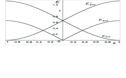
Figure 1: Energies of the BPS states given by Eqs. (17) and (18) as functions of the parameter s.

Let us now examine the presence of defects in the $s\neq 0$ case. The BPS states obey the first order equations

$$\frac{d\phi}{dx} = 1-\phi^{2}-r(\chi^{2}+\rho^{2})$$ (19)

$$\frac{d\chi}{dx} = -2r\phi\chi$$ (20)

$$\frac{d\rho}{dx} = -2r(\phi-s)\rho$$ (21)

In the sector connecting the minima $v_{1,2}$ there are topological solutions that come from a straight line orbit with $\chi=\rho=0$, which is described by $\phi(x)=\tanh(x)$. This is the one-field kink solution for the system projected into the $\phi$ axis that generates the domain wall hosting the other fields, as we referred to above. For the system projected in the $(\phi,\chi)$ plane we get the superpotential

$$W(\phi,\chi)=\phi-\frac{1}{3}\phi^{3}-r\phi\chi^{2}$$ (22)

This model was first examined in b1 , and also in b2 . In this case all the orbits in $(\phi,\chi)$ plane can be obtained explicitly, as it was recently shown in Ref. es2 .

For the system projected in the $(\phi,\rho)$ plane the superpotential is

$$W(\phi,\rho)=\phi-\frac{1}{3}\phi^{3}-r(\phi-s)\rho^{2}$$ (23)

It gives rise to the first order equations

$$\frac{d\phi}{dx} = 1-\phi^{2}-r\rho^{2}$$ (24)

$$\frac{d\rho}{dx} = -2r(\phi-s)\rho$$ (25)

To find solutions that connect the minima $v_{1,2}$ to $v_{5,6}$ we follow the approach developed in Ref. bfl . We found straight line orbits connecting these minima with

$$\rho=\pm\sqrt{\frac{1}{r}\frac{1+s}{1-s}}\,(1-\phi)$$ (26)

and

$$\rho=\pm\sqrt{\frac{1}{r}\frac{1-s}{1+s}}\,(1+\phi)$$ (27)

For the first trajectories, Eq.(26), there are BPS states for $1/r=1-s$. They are

$$\phi(x) = \frac{1}{2}(1+s)+\frac{1}{2}(1-s)\tanh(x)$$ (28)

$$\rho(x) = \pm\frac{1}{2}(1-s)\sqrt{1+s}[1-\tanh(x)]$$ (29)

They obey $\phi(x\to-\infty)\to s$ and $\rho(x\to-\infty)\to(1-s)\sqrt{1+s}$, and $\phi(x\to\infty)\to 1$ and $\rho(x\to-\infty)\to 0$. Thus, they connect $(s,0,\pm\sqrt{(1-s^{2})(1-s)})$ to $(1,0,0)$. For the second trajectories, Eq.(27), there are BPS states for $1/r=1+s$. They are

$$\phi(x) = -\frac{1}{2}(1-s)+\frac{1}{2}(1+s)\tanh(x)$$ (30)

$$\rho(x) = \pm\frac{1}{2}(1+s)\sqrt{1-s}[1+\tanh(x)]$$ (31)

They connect $(-1,0,0)$ to $(s,0,\pm\sqrt{(1-s^{2})(1+s)})$.

There are other orbits connecting the minima $v_{1,2}$ and $v_{5,6}$. We found the following parabolic trajectories

$$\rho^{2}=\frac{1}{2r}(1-s^{2})(1\pm\phi)$$ (32)

giving rise to BPS states connecting the minima for $r=1/4$. They have the form

$$\phi(x) = \frac{1}{2}(1+s)+\frac{1}{2}(1-s)\tanh[x/L^{-}(s)]$$ (33)

$$\rho(x) = \pm[2(1-s^{2})]^{1/2}\{1-\tanh[x/L^{-}(s)]\}^{1/2}$$ (34)

and

$$\phi(x) = -\frac{1}{2}(1-s)+\frac{1}{2}(1+s)\tanh[x/L^{+}(s)]$$ (35)

$$\rho(x) = \pm[2(1-s^{2})]^{1/2}\{1+\tanh[x/L^{+}(s)]\}^{1/2}$$ (36)

where $L^{\pm}(s)=2/(1\pm s)$ give the width of the topological defects.

We also found three-field BPS states connecting the minima $v_{3,4}$ to $v_{5,6}$. This is even harder, because no field can vanish along any smooth orbit connecting $v_{3,4}$ to $v_{5,6}$. We first notice that there are four different ways to connect $(0,\pm\sqrt{1/r},0)$ and $(s,0,\pm\sqrt{(1-s^{2})/r})$. We found straight line orbits described by

$$\phi\pm s\sqrt{r}\chi-s=0$$ (37)

and

$$\sqrt{\frac{1}{r}(1-s^{2})}\,\phi\mp s\rho=0$$ (38)

which imply that

$$\rho+\sqrt{1-s^{2}}\chi\mp\sqrt{\frac{1}{r}(1-s^{2})}=0$$ (39)

These orbits also project as straight line segments in each one of the three planes $(\phi,\chi)$, $(\phi,\rho)$ and $(\chi,\rho)$. We use them to rewrite Eq. (19) in the form

$$\frac{d\phi}{dx}=\frac{2}{s}\left(\phi-\frac{1}{s}\phi^{2}\right)$$ (40)

which is solved by

$$\phi(x)=\frac{s}{2}[1+\tanh(x/s)]$$ (41)

The other solutions are

$$\chi(x) = \pm\frac{1}{2}\sqrt{\frac{1}{r}}[1-\tanh(x/s)]$$ (42)

$$\rho(x) = \pm\frac{1}{2}\sqrt{\frac{1}{r}(1-s^{2})}[1+\tanh(x/s)]$$ (43)

They require that $rs^{2}=1$.

As we have shown, we have been able to find explicit BPS solutions in all the BPS sectors of a model described by three real scalar field with discrete symmetry. The presence of the parameter $s$ restricts the symmetry of the model to $Z_{2}\times Z_{2}$, since $s\neq 0$ forbids reflection symmetry along the $\phi$ axis. For this reason, now we study the behavior of the system in the limit $s\to 0$. In this case the superpotential (5) becomes

$$W=\phi-\frac{1}{3}\phi^{3}-r\phi(\chi^{2}+\rho^{2})$$ (44)

The corresponding potential supports the two minima $(\pm 1,0,0)$, and also $(0,\sqrt{1/r}\cos\theta,\sqrt{1/r}\sin\theta)$, which defines a circle in the $(\chi,\rho)$ plane for $\theta\in[0,2\pi)$. The first order equations are

$$\frac{d\phi}{dx} = 1-\phi^{2}-r(\chi^{2}+\rho^{2})$$ (45)

$$\frac{d\chi}{dx} = -2r\phi\chi$$ (46)

$$\frac{d\rho}{dx} = -2r\phi\rho$$ (47)

There are solutions connecting the minima $(\pm 1,0,0)$. One of them is given by $\chi=\rho=0$ and $\phi(x)=\tanh(x)$. Its energy is $4/3$, and it may give rise to a domain wall in $(3,1)$ space-time dimensions. There are other solutions connecting the minima $(\pm 1,0,0)$, with the same energy of the above solution. They are given by

$$\phi(x) = \tanh(2rx)$$ (48)

$$\chi(x) = \pm\sqrt{\frac{1}{r}-2\;}\frac{\cos\theta}{\cosh(2rx)}$$ (49)

$$\rho(x) = \pm\sqrt{\frac{1}{r}-2\;}\frac{\sin\theta}{\cosh(2rx)}$$ (50)

They form an elliptical surface, and in Fig. [2] we depict these solutions in the case $r=1/6$ and $\theta=\pi/6$.

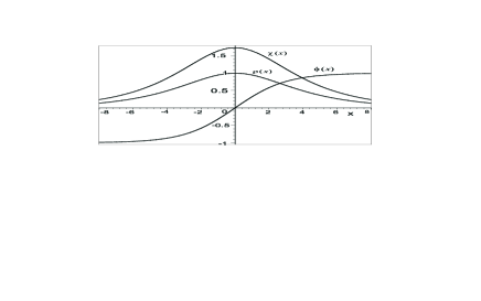
Figure 2: The BPS solution described by Eqs. (48), (49), and (50), for $r=1/6$ and $\theta=\pi/6$.

We notice that this three-field solution may be used to describe three-wave parametric solitons in quadratic nonlinear media pha . Moreover, the fact that $\chi$ and $\rho$ are non-vanishing for $x\to 0$ indicates that the wall generated by the $\phi$ field may entrap both $\chi$ and $\rho$ in its interior – see Refs. is1 ; is2 ; 00a for further details.

There are other solutions, connecting the minima $(\pm 1,0,0)$ to $(0,\sqrt{1/r}\cos\theta,\sqrt{1/r}\sin\theta)$ through parabolic surfaces. Some of them are, for $r=1/4$, and for $\chi^{2}+\rho^{2}=(1/4)(1-\phi)$

$$\phi(x) = \frac{1}{2}(1+\tanh(x/2))$$ (51)

$$\chi(x) = \pm\cos\theta\sqrt{2(1-\tanh(x/2))}$$ (52)

$$\rho(x) = \pm\sin\theta\sqrt{2(1-\tanh(x/2))}$$ (53)

and also, for $\chi^{2}+\rho^{2}=(1/4)(1+\phi)$

$$\phi(x) = -\frac{1}{2}(1-\tanh(x/2))$$ (54)

$$\chi(x) = \pm\cos\theta\sqrt{2(1+\tanh(x/2))}$$ (55)

$$\rho(x) = \pm\sin\theta\sqrt{2(1+\tanh(x/2))}$$ (56)

These solutions have the same energy, given by the value $2/3$. This is one-half the value of the energy in the former sector, defined by the minima $(\pm 1,0,0)$.

We notice that the potential generated by $W(\phi,\chi,\rho)$ as in Eq. (44) is such that

$$V(0,\chi,\rho)=\frac{1}{2}r^{2}\left(\frac{1}{r}-\chi^{2}-\rho^{2}\right)^{2}$$ (57)

It shows that the domain wall generated by the $\phi$ field may entrap the other two fields in its interior, giving rise to a model where one can have SSB of the continuum, global $U(1)$ symmetry. In Eqs. (45), (46), and (47), if we change $\chi\to\sigma\cos\theta$ and $\rho\to\sigma\cos\theta$, for $\theta$ constant we get to the equations $d\phi/dx=1-\phi^{2}-r\sigma^{2}$ and $d\sigma/dx=-2r\phi\sigma$, which are similar to the first order equations that appear in the model represented by Eq. (22), thus we can follow Ref. es2 to find all the BPS states of the model.

The continuum, global $U(1)$ symmetry that appear for $s=0$ can be further explored. For instance, we notice that in $(3,1)$ space-time dimensions the host wall $\phi(x)$ depends only on $x$, and may entrap the other two fields in two spatial dimensions. Now, if we let the continuum symmetry that appear in the $(\chi,\rho)$ plane to become local, and if we start with all the needed physical ingredients, the model gives rise to a host domain wall that entraps a planar system, driving us for instance to the scenario where the so-called Callan-Harvey effect ch may spring very naturally. We recall that the Callan-Harvey effect concerns anomaly cancelation in $(2,1)$ space-time dimensions due to the presence of a domain wall mass to a fermionic field, and we quote Ref. cha for an Abelian version of this effect. This issue is presently under investigation, and we hope to report on it in the near future.

Another line of investigation concerns the high temperature effects, which may drive the system to phase transitions. This line may follow the two last work in Ref. is2 , which deal with the thermal effects in the case of two real scalar fields. Furthermore, since the high temperature effects are obtained a la Matsubara, which is a compactification process, we can also consider more general possibilities mms , in which one investigates the effective potential in the case two or more dimensions of the original space-time are compactified. Similar ideas have been introduced in rwo for bosons and fermions, examining the temperature inversion symmetry. This direction brings other issues since together with the usual thermal effects, we are also investigating effects of compactification of one or more spatial dimensions.

The presence of topological sectors depends on the manifold of vacuum states of the system, and this indicates that our investigations are model-dependent. Thus we can build other three-field models, exploring the possibility of finding spatial junctions of defects, which may allow that we fill space with solid structures, generalizing the idea of tiling the plane with regular poligons. In the plane there are an infinity of regular polygons, although only three of them are capable of tiling the plane. In space, however, there are only five regular polyhedra – the five Platonic solids – and the issue is then which are capable of filling space, and how we can generate them within the context of three-field models. These and other related issues are presently under consideration, and we hope to report on them in the near future.

We would like to thank A.R. Gomes, J.R.S. Nascimento and R.F. Ribeiro for discussions, and CAPES, CNPq, PROCAD and PRONEX for partial support.

References

- (1) A.H. Eschenfelder, Magnetic Bubble Technology (Springer-Verlag, Berlin, 1981).
- (2) D. Walgraef, Spatio-Temporal Pattern Formation (Springer-Verlag, New York, 1997).
- (3) A. Vilenkin and E.P.S. Shellard, Cosmic Strings and Other Topological Defects (Cambridge University Press, Cambridge, UK, 1994).
- (4) E.R.C. Abraham and P.K. Townsend, Nucl. Phys. B 351, 313 (1991).
- (5) J.R. Morris and D. Bazeia, Phys. Rev. D 54, 5217 (1996); J.D. Edelstein, M.L. Trobo, F.A. Brito and D. Bazeia, Phys. Rev. D 57, 7561 (1998).
- (6) G.W. Gibbons and P.K. Townsend, Phys. Rev. Lett. 83, 1727 (1999); P.M. Saffin, Phys. Rev. Lett. 83, 4249 (1999); H. Oda, K. Ito, M. Naganuma, and N. Sakai, Phys. Lett. B 471, 140 (1999).
- (7) S.M. Carroll, S. Hellerman, and M. Trodden, Phys. Rev. D 61, 065001 (2000); D. Binosi and T. ter Veldhuis, Phys Lett. B 476, 124 (2000); M. Shifman and T. ter Veldhuis, Phys. Rev. D 62, 065004 (2000).
- (8) M. Cvetiv, S. Griffies, and S.-J. Rey, Nucl. Phys. B 381, 301 (1992); M. Cvetic and H.H. Soleng, Phys. Rep. 282, 159 (1997).
- (9) O. DeWolfe, D.Z. Freedman, S.S. Gubser, and A. Karch, Phys. Rev. D 62, 046008 (2000).
- (10) E.B. Bogomol’nyi, Sov. J. Nucl. Phys. 24, 449 (1976); M.K. Prasad and C.M. Sommerfield, Phys. Rev. Lett. 35, 760 (1975).
- (11) D. Bazeia, A.S. Inácio, and L. Losano, hep-th/0111015.
- (12) J.R. Morris, Phys. Rev. D 51, 697 (1995); 52, 1096 (1995); Int. J. Mod. Phys. A 13, 1115 (1998).
- (13) D. Bazeia, R.F. Ribeiro and M.M. Santos, Phys. Rev. D 54, 1852 (1996); F.A. Brito and D. Bazeia, Phys. Rev. D 56, 7869 (1997); D. Bazeia, H. Boschi-Filho, and F.A. Brito, J. High Energy Phys. 04, 028 (1999).
- (14) D. Bazeia and F.A.Brito, Phys. Rev. Lett. 84, 1094 (2000).
- (15) D. Bazeia and F.A. Brito, Phys. Rev. D 62, 101701(R) (2000).
- (16) F.A. Brito and D. Bazeia, Phys. Rev. D 64, 065022 (2001).
- (17) R.A. Battye and P.M. Sutcliffe, Phys. Rev. Lett. 86, 3989 (2001).
- (18) V.P. Frolov and D.V. Fursaev, Class. Quant. Grav. 18, 1535 (2001).
- (19) S. Alexander, R. Brandenberger, R. Easther, and A. Sornborger, hep-ph/9903254; M. Nagasawa and R. Brandenberger, Phys. Lett. B 467, 205 (1999).
- (20) A. Alonso Izquierdo, M.A. González León, and J. Mateos Guilarte, Nonlinearity 15, 1097 (2002).
- (21) D. Bazeia, M. J. dos Santos, and R. F. Ribeiro, Phys. Lett. A. 208, 84 (1995).
- (22) D. Bazeia, R. F. Ribeiro, and M. M. Santos, Phys. Rev. D 54, 1852 (1996); Phys. Rev. E 54, 2943 (1996); D. Bazeia, J.R.S. Nascimento, R.F. Ribeiro, and D. Toledo, J. Phys. A 30, 8157 (1997); D. Bazeia and F.A. Brito, Phys. Rev. D 61, 105019 (2000).
- (23) C.G. Callan, Jr and J.A. Harvey, Nucl. Phys. B 250, 427 (1985).
- (24) S. Chandrasekharan, Phys. Rev. D 49, 1980 (1994).
- (25) A. Alonso Izquierdo, M.A. Gonzáles León, and J. Mateos Guilarte, Phys. Rev. D 65, 085012 (2002).
- (26) D. Bazeia, W. Freire, L. Losano, and R.F. Ribeiro, hep-th/0205305.
- (27) A. Picozzi and M. Haelterman, Phys. Rev. Lett. 86, 2010 (2001).
- (28) A.P.C. Malbouisson, J.M.C. Malbouisson, and A.E. Santana, Nucl. Phys. B 631, 83 (2002).
- (29) F. Ravndal and C. Wotzasek, Phys. Lett. B 249, 266 (1990); C. Wotzasek, J. Phys A 23, 1627 (1990).