MCTP-02-25

Hagedorn Inflation: Open Strings on Branes Can Drive Inflation

Steven Abel^a,, Katherine Freese ^b,, Ian I. Kogan ^c,

$a$ Dept. of Mathematical Sciences, University of Durham, Science Laboratories, South Rd., Durham DH1 3LE, United Kingdom
$b$ Michigan Center for Theoretical Physics, University of Michigan, Ann Arbor MI 48109-1120, USA
$c$ Theoretical Physics, 1 Keble Rd, Oxford OX1 3NP, UK

Abstract

We demonstrate an inflationary solution to the cosmological horizon problem during the Hagedorn regime in the early universe. Here the observable universe is confined to three spatial dimensions (a three-brane) embedded in higher dimensions. The only ingredients required are open strings on D-branes at temperatures close to the string scale. No potential is required. Winding modes of the strings provide a negative pressure that can drive inflation of our observable universe. Hence the mere existence of open strings on branes in the early hot phase of the universe drives Hagedorn inflation, which can be either power law or exponential. We note the amusing fact that, in the case of stationary extra dimensions, inflationary expansion takes place only for branes of three or less dimensions.

1 Introduction

Inflationary cosmology [1] was proposed as a solution to the horizon, flatness, and monopole problems of the standard Hot Big Bang scenario. The cosmological horizon problem can be stated as follows: The comoving size of our observable universe today is $L_{o}=\int_{t_{dec}}^{t_{o}}{dt\over a(t)}$, where $a(t)$ is the scale factor, $t_{dec}$ is the time of radiation decoupling, and $t_{o}$ is the age of the universe today. This lengthscale must fit inside the comoving size of the horizon (a causal region) at some early time $t_{n}$ (before decoupling), $L_{n}=\int_{o}^{t_{n}}{dt\over a(t)}$. To explain causal contact of all points of our observable universe at $t_{n}$, we need $L_{o}<L_{n}$. For power law expansion of the scale factor both before $t_{n}$ and after $t_{dec}$, this condition becomes ${1\over a_{n}H_{n}}\geq{1\over a_{o}H_{o}}$ where the Hubble constant $H=\dot{a}/a$. Inflation solves this causality condition with a period of accelerated expansion, $\ddot{a}>0$, corresponding to a superluminal expansion of the scale factor. In the standard 3+1 dimensional universe, the Friedmann Robertson Walker (FRW) equations imply ${\ddot{a}\over a}=-{4\pi\over 3m_{pl}^{2}}(\rho+3p)$. Hence accelerated expansion is provided by a negative pressure. In standard inflationary models, this negative pressure is provided by a vacuum energy (a potential) with $p=-\rho$.

We have found [2] an entirely different source of negative pressure: open strings on D-branes at temperatures close to the string scale. Although Einstein’s equations in higher dimensions take a different form than the FRW equation above, negative pressure can still drive inflation. Note that there is no potential of any kind in our model; instead, open strings on branes drive the inflation.

At sufficiently high temperatures and densities fundamental strings enter a curious ‘long string’ Hagedorn phase [3, 4, 5, 6, 7, 8]. A classical random walk picture can be used to model the behaviour of the strings in cosmological backgrounds. The particular systems we will focus on are D-branes in the weak coupling limit [9]. In particular, we consider the scenario in which our observable universe is confined to three spatial dimensions (a three-brane) embedded in higher dimensions. We will denote the rest of the universe outside of our 3-brane as the bulk. We can separate the energy momentum tensor into two components: a localized component corresponding to the D-brane tension, and a diffuse component that spreads into the bulk corresponding to open string excitations of the brane. We find an interesting type of cosmological effect of a primordial Hagedorn phase of open strings on branes:

• Hagedorn inflation. The transverse ‘bulk’ components of the energy-momentum tensor can be negative. If all of the transverse dimensions have winding modes, this negative ‘pressure’ causes the brane to power law inflate along its length with a scale factor that varies as $a\sim t^{4/3}$ even in the absence of a nett cosmological constant (as shown in eq.(20)). If there are transverse dimensions that are large (in the sense that the string modes are not space-filling in these directions), then we can find exponential inflation (as shown in eq.(21)). No potential is required here. Merely the existence of open strings on D-branes drives the inflation.

We begin by discussing string thermodynamics of open strings on D-branes at high temperatures near the string scale. We argue that the features relevant to this paper can be derived by obtaining the density of states from a random walk picture. From the density of states one can derive a partition function. Then the partition function gives the energy-momentum tensor, the principal ingredient of Einstein’s equations. Winding modes of the strings give rise to a negative ‘pressure’ in the bulk (the directions perpendicular to the three-brane on which we live). This energy-momentum tensor, given in Eq.(3), is one of the most important results of the paper. Armed with the energy-momentum tensor, we examine the resultant cosmology. We can solve Einstein’s equations with various ansätze in the presence of this negative bulk component. Our primary result is that we find Hagedorn inflation of our observable universe due to the negative pressure in the bulk.

If one assumes adiabaticity, the inflationary growth period drives down the temperature of the system; eventually the temperature drop causes the universe to leave the Hagedorn regime, and consequently inflation ends automatically. In fact our solutions are only valid for small changes in the metric corresponding to small changes in the volumes, i.e., we can demonstrate instability to inflationary expansion but cannot follow the solutions further. If one uses the solutions beyond the region of their validity, the period of superluminal growth ends too quickly to solve cosmological problems. Hence we do also discuss how, in non-adiabatic systems, inflation can be sustained.

An amusing result is that power law inflation in the universal high energy system only takes place if the number of large dimensions on the brane is $p\leq 3$. In addition, branes tend to ‘melt’ unless $p\leq 4$. Hence one can speculate on the role of these effects in the fact that our observable universe has three large dimensions.

2 The Hagedorn phase and random walks

Previous work ref.[7] obtained the thermodynamic properties of D-branes in toroidal compactification using both microcanonical and canonical ensembles. The same results can be obtained from a random walk argument, where the thermodynamic properties are independent of the details of the compactification (e.g. nontoroidal) and the degree of supersymmetry. Here we will derive an expression for the partition function based on a random walk argument. The reader interested only in the result for the energy-momentum tensor and the resultant cosmology should proceed directly to Eq.(3).

2.1 String thermodynamics and the Hagedorn phase

The Hagedorn phase arises in theories containing fundamental strings because they have a large number of internal degrees of freedom. Indeed, because of the existence of many oscillator modes, the density of states grows exponentially with energy $\varepsilon$, $\omega(\varepsilon)\sim\varepsilon^{-b}e^{\beta_{H}\varepsilon}$, where the inverse Hagedorn temperature $\beta_{H}$ (where $\beta=1/T$) and the exponent $b$ depend on the particular theory in question (for example heterotic or type II) [3]. For type I,IIA,IIB strings the numerical value of the inverse Hagedorn temperature is $\beta_{H}=2\sqrt{2}\pi$ in string units. It is easy to see that thermodynamic quantities, such as the entropy, are liable to diverge at the Hagedorn temperature; obtaining the partition function $Z$ with the canonical ensemble and multiplying by the usual Boltzmann factor $e^{-\beta\varepsilon}$, one finds an integral for the partition function (for large $\varepsilon$) $Z\propto\int d\varepsilon\varepsilon^{-b}e^{(\beta_{H}-\beta)\varepsilon}$ which diverges at $\beta=\beta_{H}$ for $b\leq 2$.

In the Hagedorn regime, fundamental strings can be described as ‘long strings’ in a random walk analogy. [In a one-dimensional random walk, with each step one has 2 choices of direction (right or left) leading after ‘n’ steps to the factor $2^{n}=e^{(log2)n}$, which mimics the exponential behavior of $\omega(\varepsilon)$ above.] The size of the random walk (the distance covered by the string) is given by the length scale $\sqrt{\varepsilon}$. The physical setup is shown in Figure 1.

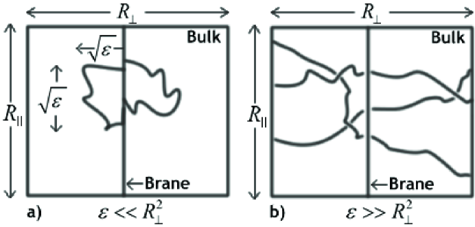
Figure 1: We consider a volume, portrayed by the box, containing a single brane embedded in the bulk. The quantity $R_{||}$ indicates the size of the dimensions parallel to the brane (for cosmology, $R_{||}\rightarrow\infty$) and $R_{\perp}$ indicates the size of the dimensions perpendicular to the brane. The random walk of strings attached to the brane traverses a distance $\sqrt{\varepsilon}$. Figs. 1a represents the case $\sqrt{\epsilon}<<R_{\perp}$. Fig. 1b represents the case $\sqrt{\epsilon}>>R_{\perp}$. This latter case is our standard high energy case in which all modes are space-filling (effectively, “winding modes”).

We consider a volume, portrayed by the box, containing a single brane. The quantity $R_{||}$ indicates the size of the dimensions parallel to the brane (for cosmology, $R_{||}\rightarrow\infty$) and $R_{\perp}$ indicates the size of the dimensions perpendicular to the brane. The random walk of strings attached to the brane traverses a distance $\sqrt{\varepsilon}$. Figs. 1a and 1b show the cases $\sqrt{\epsilon}<<R_{\perp}$ and $\sqrt{\epsilon}>>R_{\perp}$ respectively. In this paper we are particularly interested in the high energy case of fig. 1b, in which the strings fill all the space; for the case of toroidal compactification this corresponds to winding modes. We will use the nomenclature ‘winding modes’ to encompass these space-filling modes regardless of the type of compactification. We define $d_{o}$ to be the number of dimensions transverse to the brane in which there are no windings. As our standard ‘high-energy’ regime, we will take the case of $d_{o}=0$, so that all dimensions have windings; this is the system which is always reached provided that the the energy density is high enough.

In ref.[7], results for the entropy density for various limiting systems of different values of $d_{o}$ were obtained in the microcanonical ensemble working in an approximation to the thermodynamic limit. In ref.[7] a random walk interpretation with the appropriate combinatorics was also used to obtain the distribution function $\omega(\varepsilon)$ for open strings attached to a brane:

$$\omega(\varepsilon)_{\rm open}\sim{V_{\parallel}\over\varepsilon^{d_{\perp}/2}}\;\exp\,(\beta_{H}\,\varepsilon)\,\,\hskip 28.45274ptR_{\perp}\gg\sqrt{\varepsilon}\,.$$ (1)

and

$$\omega(\varepsilon)_{\rm open}\sim{V_{\parallel}\over V_{\perp}}\;\exp\,(\beta_{H}\,\varepsilon)\,\,\hskip 28.45274ptR_{\perp}\ll\sqrt{\varepsilon}.$$ (2)

One can now adapt the random walk to a cosmological background. In the case of a non-trivial metric the most natural interpretation of the parameter $\varepsilon$ is that it is the proper length of a string in the bulk and certainly we can always go to the local inertial frame in which a small portion of the string has the usual Euclidean energy $\equiv$ length equivalence.

We first make the usual quasi-equilibrium approximation that equilibrium is established much more quickly than any change in the metric so that the metric may be taken to be approximately constant in time when evaluating properties such as density. In order to simplify matters, we also assume that the metric is expressed in terms of parallel dimensions $x$ and transverse ones $y$

$$ds^{2}=-n^{2}dt^{2}+g_{||ij}dx^{i}dx^{j}+g_{\perp nm}dy^{n}dy^{m},$$ (3)

with the brane lying at $y^{n}=0$. We also define an averaging over the extra dimension with an overbar,

$$\overline{O}=\frac{\int dy\sqrt{g_{\perp}}O(y)}{\int dy^{\prime}\sqrt{g_{\perp}}}\,.$$ (4)

In [2], we found the density of states for the limiting systems to be the same expression as in the flat space case of eq. (2) but with all volumes averaged over transverse dimensions as in eq.(4).

2.2 Partition Function

Now that we have obtained a density of states of open strings attached to branes near the Hagedorn temperature, we can find the partition function at temperature $1/\beta$,

$$\log Z(\beta,\overline{V_{\parallel}},\overline{V_{\perp}})\sim\int d\varepsilon\,\,\omega(\varepsilon)\,\,e^{-\beta\varepsilon}.$$ (5)

In the standard $d_{o}=0$ case,

$$\log Z(\beta,\overline{V_{\parallel}},\overline{V_{\perp}})=2\frac{\overline{V_{\parallel}}^{2}\beta_{H}^{2}}{\overline{V_{\perp}}(\beta^{2}-\beta_{H}^{2})}+{\rm nonsingular}\,\,{\rm cutoff}\,\,{\rm terms}$$ (6)

which are the successive terms in a saddle point approximation. In [2], we present the density of states and partition function for arbitrary values of $d_{o}$ as well.

3 Stress-energy tensor $T_{\mu\nu}$ in a bulk Hagedorn phase

We now use these thermodynamic results to find the bulk energy momentum tensor during the Hagedorn regime. We may find the energy momentum tensor from

$$\langle T^{\mu}_{\nu}\rangle=2\frac{g^{\mu\rho}}{\sqrt{g}}\frac{\delta\log Z(\beta,\overline{V_{\parallel}},\overline{V_{\perp}})}{\delta g^{\rho\nu}}.$$ (7)

We will treat the functional derivative with respect to $g_{\mu\nu}$ in the following way. We assume that small changes in the metric correspond to making small changes in the volumes in $\log Z$, e.g. for a single extra dimension

$${\delta Z\over\delta g_{55}}=\int dx^{\prime}{\delta Z\over\delta\overline{V}_{\perp}(x^{\prime})}{\delta\overline{V}_{\perp}(x^{\prime})\over\delta g_{55}}\,.$$ (8)

Then, in the case of only one extra dimension, we can write

$$\overline{V_{\perp}}=\int dy\sqrt{g_{55}}={\int d^{5}x\sqrt{g_{55}}\over\int d^{4}x}={1\over v\beta}\int d^{5}x\sqrt{g_{55}}\,,$$ (9)

and

$${\delta\overline{V_{\perp}}\over\delta g_{55}}=\frac{1}{2\sqrt{g_{55}}V_{\parallel}\beta}\,.$$ (10)

Then from eqs.(8–10) we can determine the functional derivative in eq.(7). Our ansatz automatically means that $T_{05}=0$ and hence $G_{05}=0$; in other words we are not considering energy exchange between the brane and the bulk. (In general there might be energy flux between the two.)

We now summarize the results for the energy-momentum tensor. We first drop the overline notation of the previous section and simply redefine $V_{\perp}$ and $V_{\parallel}$ to be the transverse and parallel volumes covariantly averaged over the region of the transverse dimensions covered by the strings. We define an energy density $\rho$ of strings

$$\rho=\frac{E}{V_{\parallel}}$$ (11)

and define

$$\gamma=d_{o}/2-1$$ (12)

where $d_{o}$ is the number of dimensions with no windings. We find that the ‘bulk’ components of the energy momentum tensor are given by

$$\hat{T}^{0}_{0} = -\hat{\rho}$$

$$\hat{T}^{i}_{i} = \hat{p}_{\gamma}$$

$$\hat{T}^{m}_{m}\equiv p_{bulk} \approx \left\{\begin{array}[]{ll}-\hat{p}_{\gamma}&\mbox{transverse with windings}\\ 0&\mbox{transverse without windings,}\end{array}\right.$$ (15)

where $\hat{\rho}=\rho/V_{\perp}$ and

$$\hat{p}_{\gamma}=\left\{\begin{array}[]{ll}\frac{1}{V_{\perp}^{3/2}}\rho^{\frac{\gamma}{\gamma-1}}&{\rm if}\;\;\;\;{\gamma=-1,-\frac{1}{2},\frac{1}{2}}\\ \\ \frac{1}{V_{\perp}^{3/2}}\log\rho&{\rm if}\;\;\;\;{\gamma=0}\\ \\ \frac{1}{V_{\perp}^{3/2}}e^{-\rho}&{\rm if}\;\;\;\;{\gamma=1,}\end{array}\right.$$

wherever there are strings present, and zero otherwise. In particular, for our standard high energy case of $\gamma=-1$, the negative bulk pressure is:

$$p_{bulk}\sim-\rho^{1/2}/V_{\perp}^{3/2}.$$ (16)

As expected $\hat{T}_{0}^{0}$ resembles the local energy density of strings. The $\hat{T}^{i}_{i}$ represents a relatively small pressure coming from Kaluza-Klein modes in the Neumann directions and $\hat{T}^{m}_{m}$ is a negative pressure coming from winding modes in the Dirichlet directions. If we T-dualize the Dirichlet directions these ‘winding modes’ also become Kaluza-Klein modes in Neumann-directions and $T_{m}^{m}$ becomes positive. Thus negative $T_{m}^{m}$ reflects the fact that we have T-dualized a dimension much smaller than the string scale thereby reversing the pressure. For this reason negative $T_{\mu}^{\mu}$ is expected to be a general feature of space-filling excitations in transverse dimensions. The most important result of this section is the negative bulk pressure found in Eqs.(15) and (16).

4 Cosmological Equations in $D=5$

We now consider a D-brane configuration that has 3 large parallel dimensions (i.e. the ‘observable universe’) and only one transverse dimension $y$ that supports winding modes. For now, we also assume adiabaticity.

We use the metric,

$$ds^{2}=-n^{2}dt^{2}+a^{2}d{\bf x}^{2}+b^{2}dy^{2},$$ (17)

which foliates the space into flat, homogeneous, and isotropic spatial 3-planes. Here ${\bf x}=x_{1},x_{2},x_{3}$ are the coordinates on the spatial 3-planes while $y$ is the coordinate of the extra dimension. For simplicity, we make a further restriction by imposing $Z_{2}$ symmetry under $y\rightarrow-y$. Without any loss of generality we choose the 3-brane of the ‘observable universe’ to be fixed at $y=0$. We can associate a scale factor with the parallel dimensions $a(t,y)$ and one for the ‘extra’ transverse dimensions $b(t,y)$. We define $a_{0}(t(\tau))=a(t,0)$ as the scale factor describing the expansion of the 3-brane where $t(\tau)\equiv\int d\tau n(\tau,y=0)$ is the proper time of a comoving observer.

Several authors [11] - [16] have presented the bulk Einstein equations. For illustrative purposes we restate the results for the 55 (yy) equation:

$$\hat{G}_{55}=3\Biggl{\{}\frac{a^{\prime}}{a}\,\Biggl{(}\frac{a^{\prime}}{a}+\frac{n^{\prime}}{n}\Biggr{)}-\frac{b^{2}}{n^{2}}\,\Biggl{[}\frac{\dot{a}}{a}\,\Biggl{(}\frac{\dot{a}}{a}-\frac{\dot{n}}{n}\Biggr{)}+\frac{\ddot{a}}{a}\Biggr{]}\Biggr{\}}=\hat{\kappa}^{2}\,\hat{T}_{55}\,,$$ (18)

where $\hat{\kappa}^{2}=8\pi\hat{G}=8\pi/M_{5}^{3}$, $M_{5}$ is the five-dimensional Planck mass, and the dots and primes denote differentiation with respect to $t$ and $y$, respectively. As stated earlier, our ansatz implies that $T_{05}=0$ in the bulk. Shortly we will use the $T_{\mu\nu}$ appropriate to the Hagedorn regime on the right hand side of Einstein’s equations.

From Eqn.(18), one can see right away the importance of negative components of the bulk energy momentum tensor. In the case where time derivatives of $a$ dominate on the left hand side of the equation, one has ${b^{2}\over n^{2}}\Biggl{[}\Biggl{(}{\dot{a}\over a}\Biggr{)}^{2}+{\ddot{a}\over a}\Biggr{]}=-\hat{\kappa}^{2}\,\hat{T}_{55}$. One can see that accelerated expansion $\ddot{a}>0$, which is required for inflation, takes place with a negative $\hat{T}_{55}$ such as that found in Eqns.(15) and (16).

In addition to the bulk Einstein equations, we have boundary conditions (the Israel jump conditions  [11]-[16]) due to the fact that our observable brane is embedded in the bulk. We will assume that the energy momentum tensor on the boundary can be written in a perfect fluid form, $t^{0}_{0}=\rho_{br}$ and $t^{1}_{1}=-p_{br}$, where $\rho_{br}$ and $p_{br}$ are the energy density and pressure, respectively, measured by a comoving observer. For the metric in eq.(17) and the brane at a $Z_{2}$ symmetry fixed plane, the Israel conditions become

$$3[a^{\prime}/a]_{0} = -\hat{\kappa}^{2}b_{0}\rho_{br}$$

$$3[n^{\prime}/n]_{0} = \hat{\kappa}^{2}b_{0}(2\rho_{br}+3p_{br})\,.$$ (19)

In the next section, we will solve Einstein’s equations together with the constraints provided by the Israel conditions, using the energy momentum tensor we have obtained for the primordial Hagedorn regime.

Before turning to our results, let us compare the relative contributions of the stringy excitations and of the D-brane tension to the cosmology. Somewhat counterintuitively, we conclude that the diffuse stringy component can have a dominant effect on the cosmology even in the weak coupling limit (see the discussion in [2]). The intrinsic tension of the D-brane, $T_{D}\sim 1/\hat{\kappa}$, with $\hat{\kappa}\sim g_{s}$, appears large for small coupling. However, using the Israel conditions, we see that the contribution of the brane tension to terms in Einstein’s equations is of the form $\hat{\kappa}^{4}T_{D}^{2}\sim\hat{\kappa}^{2}$ while the contribution of the stringy components is $\hat{\kappa}^{2}\rho/V_{\perp}$ or $\hat{\kappa}^{2}p_{\gamma}$. Since we have assumed $\rho\leq T_{D}$ in order for the perturbative treatment of the D=brane to be valid, we see that the stringy contribution to the cosmological equations can be ${\cal O}({\hat{\kappa}})$ while that from the intrinsic tension is ${\cal O}({\hat{\kappa}}^{2})$; thus weak coupling is advantageous for string dominance in the cosmology. In addition, the Yang-Mills degrees of freedom on the brane are subdominant to the bulk degrees of freedom near $T_{H}$.

5 Results: Behaviour of scale factors $a(t)$ and $b(t)$: Inflation without Inflatons

Our results are obtained by solving Einstein’s equations together with the constraints provided by the Israel conditions. We use the energy momentum tensor derived above in Eq.(3) appropriate to a primordial Hagedorn epoch. First we will consider the case where the brane is energy/pressureless and that $\dot{b}=0$ (where $b$ is the scale factor of the extra dimension). We then catalogue more general types of behaviour that can occur for $\dot{b}\neq 0$.

5.1 Case I: $\Lambda_{br}=\Lambda_{bulk}=\dot{b}=0$

Let us first impose $\dot{b}=0$ simply as an external condition; i.e. the extra dimension is fixed in time. We also set the cosmological constants both on the brane and in the bulk to zero, $\Lambda_{br}=\Lambda_{bulk}=0$. All other contributions to the energy momentum localized on the brane (for example massless Yang-Mills degrees of freedom) have an entropy that is subdominant to the limiting bulk degrees of freedom as long as the string energy density $\rho>\rho_{c}$ (where $\rho_{c}$ is a critical Hagedorn density of order 1 in string units). For the moment we will therefore neglect the brane energy-momentum and set $a^{\prime}(t,0)=n^{\prime}(t,0)=0$. In this discussion the brane at $y=0$ is playing no role in determining the evolution of the cosmology; the scale factor $a_{0}$ changes purely as a result of the bulk equations. It is simple to solve the 55 equation for the scale factor $a_{0}(t)\equiv a(t,0)$ on our brane (at $y=0$).

Standard case with $d_{o}=0$: In the high energy case with windings in all transverse dimensions we see from Eqs.(3) and (16) that $T_{5}^{5}\sim\sqrt{\rho}\sim a^{-3/2}$ (where, again, $\rho$ is the local energy density measured with respect to the volume $V_{\parallel}$) and hence,

$$a_{0}(t)\sim t^{4/3}\,,$$ (20)

i.e. power law inflation. For the more general case of ‘p’ large parallel dimensions in any number of extra perpendicular dimensions, we find $T_{5}^{5}\sim a^{-p/2}$ and $a\sim t^{4/p}$. Here adiabaticity has been assumed in taking $E\sim S\sim{\rm const}$. We note the amusing result that inflation requires $p\leq 3$ (for our brane $p=3$) and speculate on its role in our three large extra dimensions.

Case with $d_{o}=2$: In the case of 2 dimensions with no windings, we find a period of exponential inflation:

$$\frac{a_{0}(t)}{a_{0}(0)}=\exp\left({-\frac{t^{2}\hat{\kappa}^{2}}{8V_{\perp}^{\frac{3}{2}}}+t\sqrt{\frac{\hat{\kappa}^{2}}{6V_{\perp}^{\frac{3}{2}}}\log(\rho(0)e^{3/4})}}\right)$$ (21)

where $\rho(0)$ is the initial density at $t=0$. Initially the second term in the exponent dominates and there is exponential inflation. This solution has an automatic end to inflation when $\rho(t)\sim 1$ (in string units), just as the system is dropping out of the Hagedorn phase.

Other systems: We summarize the energy momentum tensors and cosmological behavior of $a_{0}(t)$ for systems with $d_{o}$ perpendicular dimensions without windings in Table 1, where $p=3$ in our ‘toy-model’. Superluminal expansion is found for systems with $d_{o}\leq 2$, i.e., no more than two perpendicular dimensions without windings.

In adiabatic systems the Hagedorn regime and hence the inflationary behaviour we have found eventually come to an end. For a system to be in the Hagedorn regime requires an entropy density higher than the critical Hagedorn density (of order 1 in string units). Below this density the energy momentum tensor and hence the cosmology is governed by the massless relativistic Yang-Mills gas (the gas is present on the brane even in the Hagedorn regime but is subdominant). Thus there is no problem exiting from the inflationary behaviour. In fact the main issue is how long inflation can last. We return to this question later when we discuss how inflation can be sustained.

regime $\rho(\beta)=E/V_{\parallel}$ $-p_{bulk}$ $a_{0}(t)/a_{0}(0)$ $d_{o}=0$ $\frac{1}{V_{\perp}}(\beta-\beta_{H})^{-2}$ $\rho^{\frac{1}{2}}$ $t^{\frac{4}{p}}$ $d_{o}=1$ $(\beta-\beta_{H})^{-\frac{3}{2}}$ $\rho^{\frac{1}{3}}$ $t^{\frac{6}{p}}$ $d_{o}=2$ $(\beta-\beta_{H})^{-1}$ $\log\rho$ $\exp\left({-Ct^{2}+Dt}\right)$ $d_{0}=3$ $(\beta-\beta_{H})^{-\frac{1}{2}}$ $\rho^{-1}$ $t^{-\frac{2}{p}}$ $d_{0}=4$ $-\log(\beta-\beta_{H})$ $e^{-\rho}$ const

Table 1: Cosmological regimes for open strings in the Hagedorn phase with $p$ large parallel dimensions, where $p=3$ for our observable universe as a 3-brane. Here $d_{0}$ is the number of dimensions transverse to the brane in which there are no windings; in our standard “high-energy” regime we take $d_{0}=0$. Here $\rho$ is the energy density of strings, i.e. , the $T_{00}$ component of the bulk energy-momentum tensor. In addition, $T_{55}=p_{bulk}$ is the negative bulk pressure that drives inflation of our scale factor $a_{0}(t)$. Note inflationary expansion for $d_{o}\leq 2$, i.e., at most 2 directions without windings. The constants $C$ and $D$ are given for $p=3$ in eq.(21).

In all cases, we have also found solutions to the $T_{00}$ and $T_{ii}$ equations.

5.2 Case II: $\frac{\hat{\kappa}^{2}}{12}\Lambda_{br}^{2}-\Lambda_{bulk}=0$ and $\dot{b}\neq 0$

We also studied the case where the extra dimension is not stabilized but there is still no nett cosmological constant. By ‘nett’ we mean that the contribution from $a^{\prime}$ and $n^{\prime}$ in $G_{5}^{5}$ cancels the bulk contribution on the RHS of the $T_{5}^{5}$ equation. The condition for this is

$$\Lambda_{nett}=-\frac{\hat{\kappa}^{2}}{12}\Lambda_{br}^{2}+\Lambda_{bulk}=0.$$ (22)

Using the 55 equation, we catalogued some possible types of behavior for $a$ with different ansätze for $b$. Since $\alpha\approx 1$, for $\gamma=-1,-\frac{1}{2},\frac{1}{2}$ ($\gamma=d_{o}/2-1$), the pressure is

$$-p_{bulk}\propto a^{{-3\gamma}\over{\gamma-1}}b^{-3\over 2}\,.$$ (23)

Taking $\Lambda_{nett}=0$, we find a family of power law solutions for $\gamma=-1,-\frac{1}{2},\frac{1}{2}$ of the form

$$a_{0}(t) \approx At^{q}$$

$$b_{0}(t) \approx Bt^{r}$$ (24)

where subscript-0 indicates values at $y=0$,

$$q={{{\gamma-1}\over{2\gamma}}({4\over 3}-r)},$$ (25)

and $r$ is arbitrary. For our standard $\gamma=-1$, we find superluminal solutions with $q>1$ for $r<1/3$. Hence one can have an inflating brane with a shrinking bulk ($r<0$) or with a growing bulk ($0<r<1/3$). We also find a family of hyperbolic solutions with

$${a_{o}(t)\over a_{o}(0)}=\Biggl{(}{{\rm sinh}2C(t+t_{1})\over{\rm sinh}2Ct_{1}}\Biggr{)}^{1/2}.$$ (26)

These solutions can give an exponentially increasing scale factor on our brane. The proper choice of solution in Case II depends on the initial value of $\dot{b}_{o}$.

5.3 Case III: $\frac{\hat{\kappa}^{2}}{12}\Lambda_{br}^{2}-\Lambda_{bulk}\neq 0$ and $\dot{b}\neq 0$

In [2] we also consider the case of additional cosmological constants in the brane and bulk. The results can be found in our longer paper. Not surprisingly we recover the usual cosmological constant driven inflation when we set $\rho=0$.

6 Sustaining inflation and solving the Horizon Problem

In the previous sections we have found the onset of inflation via superluminal growth of the scale factor. We also know that eventually, once the temperature drops out of the Hagedorn regime, inflation ends. This graceful exit from inflation is an appealing feature of this scenario. However, we cannot calculate in between. Once inflation begins, our calculations break down; our interpretation of small changes in the metric corresponding to small changes in volume no longer holds. At this point we can only speculate what happens in between. The following are three of the possibilities:

First, previous authors have argued that strings in a de Sitter background are unstable to fluctuations and that this instability can sustain a period of de Sitter inflation [20, 21, 22]. This phenomenon is well known for strings once they are in the de Sitter-like phase. However the missing ingredient that the present study adds is an explanation for how the universe enters a de Sitter like phase in the first place. Our mechanism gets the universe into the locally de Sitter phase, whereupon the mechanism of refs.[20, 21, 22] keeps it there without having to assume adiabaticity.

Second, our 3-brane sits in a bath of branes and bulk strings with ongoing dynamics such as branes smashing into each other and possibly annihilating. The dynamics is likely to keep the system hot. Hence high temperatures near the Hagedorn temperature may be sustained for a long period; inflation continues during this period. We note that the high entropy of our brane $S\sim 10^{88}$ may originate from the dynamics of this hot brane/string bath. Eventually the system cools, drops out of the Hagedorn regime, and inflation ends. We are investigating this scenario in a future paper.

Third, we suggest as a possible direction for future study, a metric in which each 4 dimensional leaf of the foliated space is a de Sitter space. It is well established (see for example ref.[23] and references therein) that the combined (geometric plus thermal) system obeys a generalized second law which is that the total entropy,

$$S=S_{matter}+S_{horizon}=S_{matter}+\frac{1}{4\hat{\kappa}^{2}}A_{horizon},$$ (27)

obeys $\delta S>0$, where $A_{horizon}$ is the area of the horizon. The generalized second law indicates that fluctuations in the geometry tend to drive the universe even further into the de Sitter phase provided that the Hubble constant is greater than the critical value. The entropy that the horizon loses when the Hubble constant is increased is more than offset by the huge increase in string entropy. Moreover, since the specific heat of the string gas becomes larger when the temperature increases, inevitably equilibrium is lost and energy flow to the strings becomes apparently limitless.

There is a slight difference between our study and the results of ref.[21] which we should comment on. In ref.[21], the density never goes above a critical density, $\rho^{\prime}_{c}$, and indeed asymptotes to it from below as one goes back in time. In our case, on the other hand, we must have $\rho>\rho_{c}\sim 1$ for the calculation to be valid (i.e. to be in the Hagedorn regime). Indeed in the present paper the energy density diverges as we approach the Hagedorn temperature. The difference is because ref.[21] was concerned with stretched strings and introduced a cut-off in the momentum integral in order to find the fractal dimension of the string. This ‘coarse graining’ put an artificial upper limit on the amount of string that can be packed into the volume. In fact they found the maximum fractal dimension (i.e. 2) only at the critical density $\rho^{\prime}_{c}$. A fractal dimension of 2 is typical of the random walk behaviour which exists once Hagedorn behaviour sets in. So the coarse graining in ref.[21] effectively removed the Hagedorn behaviour and consequently ref.[21] found that $\rho=\rho^{\prime}_{c}$ gave $\beta=\beta_{H}$. Conversely, the present paper begins in the regime $\rho>\rho_{c}$ where the calculations of ref.[21] end.

7 Conclusion and discussion

We have studied the possible cosmological implications of the Hagedorn regime of open strings on D-branes in the weak coupling limit. Our main result is that a gas of open strings can exhibit negative pressure leading naturally to a period of power law or even exponential inflation. Hagedorn inflation also has a natural exit since any significant cooling can cause a change in the thermodynamics if winding modes become quenched or if the density drops below the critical density, $\rho_{c}\sim 1$, needed for the entropy of the Hagedorn phase to be dominant. To summarize, open strings on branes in the hot early Hagedorn phase of the universe provide a mechanism to drive a period of inflation, even in the absence of any potential.

Acknowledgements

We thank Dan Chung, Cedric Deffayet, Emilian Dudas, Keith Olive, Geraldine Servant and Carlos Savoy for discussions. S.A.A. and I.I.K. thank Jose Barbón and Eliezer Rabinovici for a previous collaboration and discussions concerning this work. S.A.A. thanks the C.E.A. Saclay for support during this work. K.F. acknowledges support from the Department of Energy through a grant to the University of Michigan. K.F. thanks CERN in Geneva, Switzerland and the Max Planck Institut fuer Physik in Munich, Germany for hospitality during her stay. I.I.K. was supported in part by PPARC rolling grant PPA/G/O/1998/00567, the EC TMR grant FMRX-CT-96-0090 and by the INTAS grant RFBR - 950567.

References

- [1] A. Guth, Phys. Rev. D 23, 347 (1981)
- [2] S.A. Abel, K. Freese, and I.I Kogan, JHEP 0101 (2001) 039
- [3] R. Hagedorn, Suppl. Nuovo Cimento 3 (1965) 147; S. Frautschi, Phys. Rev. D 3, 2821 (1971); R.D. Carlitz, Phys. Rev. D 5, 3231 (1972)
- [4] K. Huang and S. Weinberg, Phys. Rev. Lett. 25, 895 (1970); E. Alvarez, Phys. Rev. D 31, 418 (1985); Nucl. Phys. B269, 596 (1986); M. Bowick and L.C.R. Wijewardhana, Phys. Rev. Lett. 54, 2485 (1985); B. Sundborg, Nucl. Phys. B254, 883 (1985); S.N. Tye, Phys. Lett. 158B, 388 (1985); P. Salomonson and B. Skagerstam, Nucl. Phys. B268, 349 (1986); Physica A158 (1989) 499; E. Alvarez and M.A.R. Osorio, Phys. Rev. D 36, 1175 (1987); D. Mitchell and N. Turok, Phys. Rev. Lett. 58, 1577 (1987); Nucl. Phys. B294, 1138 (1987); I. Antoniadis, J. Ellis and D.V. Nanopoulos, Phys. Lett. 199B, 402 (1987); M. Axenides, S.D. Ellis and C. Kounnas, Phys. Rev. D 37, 2964; (1988); I.I. Kogan, JETP. Lett. 45 (1987) 709; B.Sathiapalan, Phys. Rev. D 35, 3277 (1987); J. Atick and E. Witten, Nucl. Phys. B310, 291 (1988); A.A. Abrikosov Jr. and Ya. I. Kogan Int. J. Mod. Phys. A6 (1991) 1501 (submitted 1989), Sov. Phys. JETP 69 (1989) 235; R. Brandenberger and C. Vafa, Nucl. Phys. B316, 391 (1989); M.J. Bowick and S.B. Giddings, Nucl. Phys. B325, 631 (1989); S.B. Giddings, Phys. Lett. 226B, 55. (1989); R. Brandenberger and C. Vafa, Nucl. Phys. B316, 391. (1989); F. Englert and J. Orloff, Nucl. Phys. B334, 472 (1990); B.A. Campbell, J. Ellis, S. Kalara, D.V. Nanopoulos, K.A. Olive, Phys. Lett. 255B, 420 (1991); B.A. Campbell, N. Kaloper, K.A. Olive, Phys. Lett. 277B, 265 (1992); S.A. Abel, Nucl. Phys. B372, 189 (1992); N. Kaloper, K.A. Olive, Astropart.Phys.1 (1995) 185; N. Kaloper, R. Madden, K.A. Olive, Phys. Lett. 371B, 34, (1996), hep-th/9510117; N. Kaloper, R. Madden, K.A. Olive, Nucl. Phys. B452, 677, (1995) hep-th/9506027; M.L. Meana, M.A.R. Osorio and J.P. Penalba, Phys. Lett. 400B, 275, (1997) hep-th/9701122; Phys. Lett. 408B, 183 (1997) hep-th/9705185; K.R. Dienes, E. Dudas, T. Gherghetta and A. Riotto, Nucl. Phys. B543, 387 (1999)
- [5] N. Deo, S. Jain and C.-I. Tan, Phys. Lett. 220B, 125 (1989); Phys. Rev. D 40, 2646 (1989); N. Deo, S. Jain, O. Narayan and C.-I. Tan, Phys. Rev. D 45, 3641 (1992)
- [6] D.A. Lowe and L. Thorlacius, Phys. Rev. D 51, 665 (1995), hep-th/9408134; S. Lee and L. Thorlacius, Phys. Lett. 413B, 303 (1997), hep-th/9707167
- [7] J.L.F. Barbón, I.I. Kogan and E. Rabinovici, Nucl. Phys. B544, 1999 (104), hep-th/9809033; S.A. Abel, J.L.F. Barbón, I.I. Kogan, and E. Rabinovici, JHEP 04 (1999) 015
- [8] M.L. Meana and J.P. Penalba, Nucl. Phys. B560, 154 (1999); Phys. Lett. 447B, 59 (1999); M.A. Vazquez-Mozo, Phys. Rev. D 60, 106010 (1999); B. Sundborg, hep-th/9908001; S.A. Abel, J.L.F. Barbón, I.I. Kogan, and E. Rabinovici, hep-th/9911004
- [9] For reviews see: J. Polchinski, TASI lecturs on D-branes, hep-th/9611050; “String Theory”, vols 1,2 (CUP) 1998; C. Bachas, “Lectures on D-branes”, hep-th/9806199
- [10] S.A. Abel and E. Dudas, in preparation
- [11] P. Kanti, I. I. Kogan, K. A. Olive, M. Pospelov, Phys.Lett. B468 (1999) 31, hep-ph/9909481; hep-ph/9912266
- [12] K. Benakli, Int. J. Mod. Phys. D8 (1999) 153, hep-th/9804096; N. Arkani-Hamed, S. Dimopoulos and G. Dvali, Phys. Rev. D59, 086004 (1999), hep-ph/9807344; H.S. Reall, Phys. Rev. D 59, 103506, (1999) hep-th/9809195; N. Kaloper and A. Linde, Phys. Rev. D59 (1999) 101303, hep-ph/9811141; G. Dvali and S.H.H. Tye, Phys. Lett. 450B, 72 (1999), hep-ph/9812483; A. Lukas, B.A. Ovrut and D. Waldram, hep-th/9902071; T. Banks, M. Dine and A. Nelson, hep-th/9903019; H.A. Chamblin and H.S. Reall, Nucl. Phys. B562, 133 (1999), hep-th/9903225; N. Arkani-Hamed, S. Dimopoulos, N. Kaloper and J. March-Russell, hep-ph/9903224; hep-ph/9903239; P. Binétruy, C. Deffayet and D. Langlois, hep-th/9905012; N. Kaloper, Phys. Rev. D60 (1999) 123506, hep-ph/9905210; T. Nihei, Phys. Lett. B465 (1999) 81, hep-ph/9905487; C. Csáki, M. Graesser, C. Kolda and J. Terning, Phys. Lett. B462 (1999) 34, hep-ph/9906513; J.M. Cline, C. Grojean and G. Servant, Phys. Rev. Lett. 83 (1999) 4245, hep-ph/9906523
- [13] D. Chung and K.T. Freese, Phys. Rev. D 61, 023511 (2000), hep-ph/9906542
- [14] W.D. Goldberger and M.B. Wise, Phys. Rev. D60 (1999) 107505, hep-ph/9907218; Phys. Rev. Lett. 83, 4922 (1999), hep-ph/9907447; H.B. Kim and H.D. Kim, Phys. Rev. D 61, 064003 (2000), hep-th/9909053
- [15] U. Ellwanger, hep-th/9909103
- [16] T. Shiromizu, K. Maeda and M. Sasaki, gr-qc/9910076; C. Grojean, J. Cline and G. Servant, hep-th/9910081; P. Kraus, hep-th/9910149; P. Binétruy, C. Deffayet, U. Ellwanger and D. Langlois, hep-th/9910219; A. Kehagias and E. Kiritsis, JHEP 9911 (1999) 022; E. Flanagan, S.H.H. Tye and I. Wasserman, hep-ph/9910498; D. Ida, gr-qc/9912002; C. Csáki, M. Graesser, L. Randall, and J. Terning, hep-ph/9911406; W.D. Goldberger and M.B. Wise, hep-ph/9911457
- [17] O. Aharony, S. S. Gubser, J. Maldacena, H. Ooguri and Y. Oz, hep-th/9905111
- [18] C. Deffayet, private communication
- [19] , D. Chung and K. Freese, Phys. Rev. D 62, 023511 (2000)
- [20] R. Brout, F. Englert and E. Gunzig, Ann. Phys. 115 (1978) 78; Gen. Rel. Grav. 10 (1979) 1; R. Brout, F. Englert and P. Spindel, Phys. Rev. Lett. 43, 417 (1979); Y. Aharanov and A. Casher, Phys. Lett. 166B, 289 (1986); Y. Aharonov, F. Englert and J. Orloff, Phys. Lett. 199B, 366 (1987)
- [21] N.Turok, Phys. Rev. Lett. 60, 549 (1988)
- [22] N. Sanchez and G. Veneziano, Nucl. Phys. B333 (1990) 253; M. Gasperini, N. Sanchez and G. Veneziano, Int. J. Mod. Phys. A6 (1991) 3853; Nucl. Phys. B364 (1991) 365;
- [23] R. Brustein, S. Foffa and R. Sturani, Phys. Lett. B471 (2000) 352, hep-th/9907032; R. Brustein, gr-qc/9904061
- [24] A. Riotto, hep-ph/9904485
- [25] E. Alvarez, T. Ortin, Mod.Phys.Lett.A7 (1992) 2889; A. A. Bytsenko, K. Kirsten and S. Zerbini, Phys. Lett. B304 (1993) 235; A.A. Bytsenko and S.D. Odintsov, Prog. Theor. Phys. 98 (1997) 987; I.R. Klebanov and A.A. Tseytlin, Nucl. Phys. B479 (1996) 319; J.P. Penalba, Nucl. Phys. B556, 152 (1999)