Abstract

We examine a large $N$ duality via geometric transition for ${\cal N}=1$ $SO/Sp$ gauge theories with superpotential for adjoint chiral superfield. In this paper, we find that the large $N$ gauge theories are exactly analyzed for the classical quartic superpotentials by the finite rank $SO/Sp$ gauge theories. With this classical superpotentials, we evaluate the confining phase superpotentials using the Seiberg-Witten theory. In the dual theory, we calculate the superpotential generated by the R-R and NS-NS 3-form fluxes. As the non-trivial examples, we discuss for $SO(6)$, $SO(8)$ and $Sp(4)$ gauge theories. In these cases we have the perfect agreement of the confining phase superpotentials up to the 4th order of the glueball superfields.

1 Introduction

It has been conjectured that the large $N$ gauge theory describes the string theory [1]. The most prominent example of this large $N$ duality is $AdS/CFT$ correspondence [2]. As an example, Type IIB string theory on $AdS_{5}\times T^{1,1}$ realizes $\mathcal{N}=1$ supersymmetric gauge theory with conformal symmetry in large $N$ limit, and the field theory results are reproduced from the supergravity [3]. In [4], the breaking of the conformal symmetry of this model can be discussed by introducing the fractional branes.

As a large $N$ duality for topological string theory, gauge theory/geometry correspondence is proposed [5]. Via conifold transition, this duality claims that the topological string theory on the resolved conifold is equivalent to the topological string theory on the deformed conifold with $N$ A-branes wrapped on the special Lagrangian $3$-cycle in the large $N$ limit.

This topological string duality is extended to the large $N$ duality for the superstring theory [6] and M-theory [7][8]. For Type IIB string theory, T-duality reverses the direction of the transition [6][9]. The duality claims that the string theory on the resolved conifold with $N$ D$5$-branes wrapped on the exceptional ${\bf P}^{1}$ is equivalent to that on the deformed conifold with $N$ units of $3$-form fluxes through the special Lagrangian $3$-cycle $S^{3}$ in large $N$ limit. Here the fluxes on the defomed conifold generate the superpotential and break the supersymmetry spontaneously [10]. Therefore, an ${\cal N}=2$ vector multiplet splits into an ${\cal N}=1$ chiral and a vector multiplet. Especially, this chiral superfield is identified with the glueball superfield in the confining phase of the gauge theory realized on the $N$ D$5$-branes in the large $N$ limit. Under this identification, the superpotential generated by $3$-form fluxes on the deformed conifold coincides with that of the massive glueball superfield [11] in the gauge theory. In this way, the validity of the duality is examined for this geometry.

Applying the conifold transition locally, the duality is also considered for more complicated geometries [12][13][14]. In [12], the geometric transition for ${\cal O}(-2)\oplus{\cal O}(0)$ bundle over ${\bf P}^{1}$ is discussed. In the resolved geometry, classical superpotential for $U(N)$ adjoint chiral superpotential arises in the gauge theory on $N$ D5-branes wrapping on the exceptional ${\bf P}^{1}$’s, and it leads to ${\cal N}=1$ supersymmetric theory. After the geometric transition, $n$ exceptional ${\bf P}^{1}$’s shrink and $n$ $S^{3}$’s are replaced in the dual theory. Thus the dual theory is defined on the deformed geometry. On this dual geometry, $3$-form fluxes appear on $S^{3}$’s after the transition and generate superpotential. When the above duality conjecture is applied, the superpotential in the dual theory is also identified with the effective one for the original gauge theory in large $N$ limit. For some examples, the confining phase superpotentials for both theories coincides perfectly [12].

By introducing orientifold projection, the conifold is resolved by ${\bf RP}^{2}$ and the gauge group becomes $SO(N)/Sp(N)$. The large $N$ duality of unoriented string is examined for the topological string theory [15][16] and Type IIB superstring theory [17][18][19]. In [17], the geometric transition for $SO(N)$ gauge theory is discussed in this set up. As in $U(N)$ gauge theory case, The world-volume theory of $N$ D5-branes wrapped on ${\bf RP}^{2}$ realize $SO(N)/Sp(N)$ gauge theory with arbitrary classical superpotential for the adjoint chiral superfield. In order to confirm the duality proposal for this case, it is also necessary to examine the coincidence of the physical quantities on both theories. In [17], it is found that the effective coupling constant of $SO(N)$ gauge theory agrees with that of the dual theory.

In order examine the duality for $SO/Sp$ gauge theories further, we evaluate the confining phase superpotentials on both theories in this paper. On the gauge theory side, we need to evaluate it in large $N$ limit of $SO(N)/Sp(N)$ gauge group. We prove that it can be evaluated exactly from the finite rank gauge theory for the $SO/Sp$ gauge theory with the classical quartic superpotential for adjoint chiral superfield. On the dual theory side, we evaluate the periods for the deformed geometry with the orientifolding. By identifying the periods with the expectation values of the gluon superfields, we obtain the effective superpotentials. To evaluate the superpotentials explicitly on both sides, we consider $SO(6)$, $SO(8)$ and $Sp(4)$ gauge theories as the non-trivial examples. As a result, we find the perfect agreement of these superpotentials up to the 4th order of the glueball superfields.

This paper is organized as follows. In section 2, we will review the geometric transition [6] and see how the gauge theory and the string theory are exactly analyzed [12][17]. In section 3, we will prove that the confining phase superpotential for $SO(2N)/Sp(2N)$ gauge theory in the large $N$ limit is exactly evaluated from the finite rank gauge theory with the classical quartic superpotential. And then we will compute the confining phase superpotential using the Seiberg-Witten theory for the gauge groups $SO(6)$, $SO(8)$ and $Sp(4)$. In section 4, we will explicitly analyze the dual geometry and evaluate the effective superpotential from the computation of the periods. By comparing the results of section 3 and section 4, we will find the coincidence of the exact superpotentials. In the Appendix we will show the detailed computations of periods in section 3.

2 Geometric Transition and Large $N$ Duality

2.1 The Geometric Transition

We consider Type IIB string theory on non-compact Calabi-Yau manifold,

$$M_{s}:\,W^{\prime}(x)^{2}+y^{2}+z^{2}+w^{2}=0,$$ (2.1)

where $W(x)$ is defined as,

$$W(x)\equiv\sum_{p=1}^{n+1}\frac{g_{p}}{p}x^{p}.$$ (2.2)

This Calabi-Yau manifold is resolved by locating ${\bf P}^{1}$’s at the singularities where $W^{\prime}(x)=0$ is satisfied, and defined as ${\cal O}(-2)\oplus{\cal O}(0)$ bundle over ${\bf P}^{1}$. When $N$ D$5$-branes wraps on the exceptional ${\bf P}^{1}$’s and fill the flat $4$ dimensional space-time, $4$ dimensional ${\cal N}=1$ supersymmetric $U(N)$ gauge theory with superpotential $W_{{\rm cl}}$ for the adjoint chiral superfield $\Phi$,

$$W_{\rm cl}(\Phi)=\sum_{p=1}^{n+1}\frac{g_{p}}{p}{\rm Tr}\Phi^{p},$$ (2.3)

is realized [20].

In order to realize $SO(N)/Sp(N)$ gauge theories, we introduce orientifold projection which is complex conjugation. For singular geometry (2.1) this projection acts as

$$(x,y,z,w)\to(\bar{x},\bar{y},\bar{z},\bar{w}).$$ (2.4)

To extend this projection to the resolved geometry we consider new variables,

$$a=x+iy,\ \ b=z+iw,\ \ c=x-iy,\ \ d=-z+iw.$$ (2.5)

The complex conjugation (2.4) corresponds to the following action,

$$a\to\bar{c},\ \ b\to-\bar{d},\ \ c\to\bar{a},\ \ d\to-\bar{b}.$$ (2.6)

The resolved conifold can be described as a union of two patch, $M_{1}=\{(a,b,c,z)|d=ac\}$ and $M_{2}=\{(a^{\prime},b^{\prime},c^{\prime},z^{\prime})|c^{\prime}=b^{\prime}d^{\prime}\}$ glued together by the identification $b=a^{\prime}b^{\prime}$. The singular point of the Calabi-Yau manifold is replaced by ${\bf P^{1}}$ whose coordinates are given by $a^{\prime}$ on $M_{1}$ and $b^{\prime}$ on $M_{2}$. By the orientifolding (2.6) we identify $a^{\prime}$ with $-\bar{b}^{\prime}$. This is antipodal map, then ${\bf P^{1}}$ becomes ${\bf RP^{2}}$.

In this geometry world-volume theory on the D5-brane is $SO/Sp$ gauge theory with the following tree level superpotential [17],

$$W_{\mathrm{cl}}(\Phi)=\sum_{p=1}^{n+1}\frac{g_{2p}}{2p}{\rm Tr}\Phi^{2p}\equiv\sum_{p=1}^{n+1}g_{2p}u_{2p},$$ (2.7)

where $\Phi$ is the chiral superfield in the adjoint representation of $SO(N)/Sp(N)$ gauge group and $u_{2p}\equiv\frac{1}{2p}{\rm Tr}\Phi^{2p}$.

We define parameters $a_{i}$ by

$$W^{\prime}(x)=\sum_{p=1}^{n}g_{2p}x^{2p-1}=g_{2n+2}\ x\prod_{i=1}^{n}(x^{2}+a_{i}^{2}).$$ (2.8)

In the classical vacua of this gauge theory, the eigenvalues of $\Phi$ become roots $0,\pm ia_{i}$’s of $W^{\prime}(x)=0$. When $N_{0}$ D5-branes wrap on ${\bf RP}^{2}$ and $N_{i}$ D5-branes wrap on the ${\bf P}^{1}$ located at $x=\pm ia_{i}$, the vacuum of the gauge theory becomes classically $P(x)\equiv{\rm det}(x-\Phi)=x^{N_{0}}\prod_{i=1}^{n}(x^{2}+a_{i}^{2})^{N_{i}}$ and the gauge group breaks as,

$$SO(N)\to SO(N_{0})\otimes_{i=1}^{n}U(N_{i}),\quad Sp(N)\to Sp(N_{0})\otimes_{i=1}^{n}U(N_{i}),$$

where $N=N_{0}+\sum_{i=1}^{n}N_{i}$. This theory can be analyzed non-perturbatively in terms of the Seiberg-Witten theory [21][22] and we will review in the next section.

The large $N$ dual of this theory is found via conifold transition [5][6]. The conifold is defined as [23][24],

$$x^{2}+y^{2}+z^{2}+w^{2}=0.$$ (2.9)

This geometry has a singularity at $x=y=z=w=0$. This singularity can be removed in two ways. One way is the deformation of Kähler structure. This singularity is blown up and replaced by ${\bf P}^{1}$. The resulting geometry becomes ${\cal O}(-1)\oplus{\cal O}(-1)$ bundle over ${\bf P}^{1}$, and this is called resolved conifold. Another way is the deformation of the complex structure, where the defining equation is deformed as,

$$x^{2}+y^{2}+z^{2}+w^{2}=\mu^{2}.$$ (2.10)

Thus the singularity is replaced by $S^{3}$ with the radius $\mu$ and resulting geometry becomes $T^{*}S^{3}$. This manifold is called deformed conifold. When $N$ D5-branes are wrapped on ${\bf P}^{1}$ in the resolved conifold, D5-branes disappear and $N$ units of R-R $3$-form flux $H_{R}$ through $S^{3}$ and NS-NS $3$-form flux $H_{NS}$ through the dual $3$-cycle remain after the conifold transition. In the large $N$ limit, these two theories are equivalent and give the same physical quantities [6]. After the conifold transition, D$5$-branes and orientifold plane disappear and $N\mp 2$ units of R-R $3$-form flux $H_{R}$ through $\mathbf{S}^{3}$ and NS-NS $3$-form flux $H_{NS}$ through the dual $3$-cycle remain .

In the case of the Calabi-Yau manifold (2.1), above analysis can be applied locally. Through the geometric transition, the dual Calabi-Yau manifold is defined by replacing all ${\bf P}^{1}$’s and a ${\bf RP}^{2}$ by $S^{3}$’s. The deformed geometry is the following hypersurface in ${\bf C}^{4}$,

$$M_{{\rm cpx}}:\,g\equiv W^{\prime}(x)^{2}+f_{2n-2}(x)+y^{2}+z^{2}+w^{2}=0,$$ (2.11)

where $f_{2n-2}(x)$ is the degree $(n-1)$-th polynomial of $x^{2}$. In this deformed geometry, the integral basis of the $3$-cycles $A_{i},B_{i}\in H_{3}(M,{\bf Z})$ ($i=1,\cdots,h_{2,1}=2n+1$) satisfy the symplectic pairing,

$$(A_{i},B_{j})=-(B_{j},A_{i})=\delta_{ij}\ ,\qquad(A_{i},A_{j})=(B_{i},B_{j})=0,$$ (2.12)

where the pairing $(A,B)$ of three-cycles $A,B$ is defined as the intersection number. For the deformed Calabi-Yau manifold (2.11), these $3$-cycles are constructed as $\mathbf{P}^{1}$ fibration over the line segments between two critical points $x=0^{+},0^{-},\pm ia_{1}^{+},\pm ia_{1}^{-}\cdots\pm ia_{n}^{+},\pm ia_{n}^{-},\infty$ of $W^{\prime}(x)^{2}+f_{2n-2}(x)$ in $x$-plane. Therefore we set the three cycle $A_{0}$ to be the ${\bf P}^{1}$ fibration over the line segment between $0^{-}$ and $0^{+}$ and three cycle $A_{i}$ to be the fibration over the line segment between $ia_{i}^{-}$ and $ia_{i}^{+}$. On the other hand, three cycle $B_{0}$ is constructed as ${\bf P}^{1}$ fibration over the line segment between $0^{+}$ and $\Lambda_{0}$ and three cycle $B_{i}$ to be the fibration over the line segment between $ia_{i}^{+}$ and $i\Lambda_{0}$, Here we introduced the cut-off $\Lambda_{0}$, as these cycles are non-compact. Since this geometry has $\mathbf{Z}_{2}$ symmetry, the discussion is restricted to the upper half of $x$-plane in the following [17].

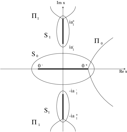
Figure 1: The 3-cycles which are constructed as the ${\bf P}^{1}$ fibration over the line segments in the complex plane.

The holomorphic $3$-form $\Omega$ for the deformed geometry (2.11) is given by

$$\Omega=2\frac{dx\wedge dy\wedge dz}{\partial g/\partial w}.$$ (2.13)

The periods $S_{i}$ and dual periods $\Pi_{i}$ for this deformed geometry is given as,

$$S_{i}=\int_{A_{i}}\Omega,\quad\Pi_{i}=\int_{B_{i}}\Omega.$$ (2.14)

The dual periods are expressed in terms of the prepotential ${\mathcal{F}}(S_{i})$ such as,

$$\Pi_{i}=\partial{\cal F}/\partial S_{i}.$$ (2.15)

Since these $3$-cycles are constructed as ${\bf P}^{1}$ fibrations, these periods are written in terms of the integrals over $x$-plane as,

$$S_{0}=\frac{1}{2\pi i}\int_{0^{-}}^{0^{+}}\omega,\quad S_{i}=\frac{1}{2\pi i}\int_{ia_{i}^{-}}^{ia_{i}^{+}}\omega,$$

$$\Pi_{0}=\frac{1}{2\pi i}\int_{0^{+}}^{\Lambda_{0}}\omega,\quad\Pi_{i}=\frac{1}{2\pi i}\int_{ia_{i}^{+}}^{i\Lambda_{0}}\omega,$$ (2.16)

where $\omega$ is obtained by integrating holomorphic $3$-form over the fiber ${\bf P}^{1}$,

$$\omega=2dx\ \left(W^{\prime}(x)^{2}+f_{2n-2}(x)\right)^{\frac{1}{2}}.$$ (2.17)

2.2 Partial SUSY Breaking and Confinement of Gauge Theory

When the geometric transition occurs, the exceptional ${\bf P}^{1}$’s on which D$5$-branes wrap in the resolved geometry, is replaced by $3$-form fluxes through the special Lagrangian $3$-cycles in the deformed geometry. This $3$-form fluxes generate the superpotential, and ${\mathcal{N}}=2$ supersymmetry for the dual theory is broken partially to ${\mathcal{N}}=1$ supersymmetry [10]. In this subsection, we will review how the partial supersymmetry breaking occurs in the dual geometry and how the supermultiplets in the dual theory are identified with that of the effective gauge theory by the large $N$ duality conjecture [6].

The partial supersymmetry breaking of ${\cal N}=2$ theory to ${\cal N}=1$ theory occurs by the electric and magnetic Fayet-Iliopoulous superpotential terms as [25],

$$W_{\mathrm{FI}}=\sum_{i}\int d\theta^{2}d\tilde{\theta}^{2}\left(e_{i}\Psi_{i}+m_{i}\frac{\partial{\cal F}}{\partial\Psi_{i}}\right),$$ (2.18)

where $e_{i}$’s and $m_{i}$’s are electric and magnetic charge respectively, and $\Psi_{i}$’s are ${\cal N}=2$ superfields and the holomorphic function ${\cal F}$ is the prepotential for the ${\cal N}=2$ theory.

Turning on R-R and NS-NS fluxes through the special Lagrangian $3$-cycles, the above partial supersymmetry breaking is realized in Type IIB string theory [10]. The $3$-form fluxes generate the superpotential [26]

$$-\frac{1}{2\pi i}W_{{\rm eff}}=\int\Omega\wedge(H_{{\rm R}}+\tau H_{{\rm NS}}),$$ (2.19)

where $H_{R}$ and $H_{NS}$ are $3$-form fluxes and $\tau$ is the complexified Type IIB string coupling, and $\Omega$ is the holomorphic $3$-form on the Calabi-Yau manifold. In the case of dual theory defined through geometric transition, $H_{\rm R}$ and $H_{NS}$ satisfy,

$$N_{0}\mp 2=\int_{A_{0}}H_{{\rm R}},\quad N_{i}=\int_{A_{i}}H_{{\rm R}},\quad\alpha=\int_{B_{i}}H_{{\rm NS}},$$ (2.20)

where $\alpha$ is the $4$ dimensional bare gauge coupling constant $g_{0}$ as $\alpha\equiv 4\pi i/g_{0}^{2}$.

Plugging these relations into (2.19), the superpotential for the dual theory is expressed in terms of periods $S_{i}$ and dual periods $\Pi_{i}$ of the deformed Calabi-Yau manifold such as,

$$-\frac{1}{2\pi i}W_{{\rm eff}}=\left(\frac{N_{0}}{2}\mp 1\right)\Pi_{0}+\sum_{i=1}^{n}N_{i}\Pi_{i}+\alpha\sum_{i=0}^{n}S_{i}.$$ (2.21)

With this superpotential, ${\cal N}=2$ vector multiplets $\Psi_{i}$ splits into the massive ${\cal N}=1$ chiral superfields $S_{i}$ and massless $U(1)^{n}$ vector multiplets. Following the large $N$ duality proposal [6], massless $U(1)^{n}$ vector multiplets are identified with those in the effective theory of the ${\cal N}=1$ $SO(N)/Sp(N)$ gauge theory with the classical superpotential $W_{{\rm cl}}(\Phi)$. The ${\cal N}=1$ massive chiral superfield $S_{i}$ is identified with the glueball superfield,

$$S_{i}=-\frac{1}{32\pi^{2}}{\rm Tr}_{SU(N_{i})}W_{\alpha}W^{\alpha},$$ (2.22)

where $W_{\alpha}$ is defined as $W_{\alpha}\equiv D_{\alpha}V$ with supercovariant derivative $D_{\alpha}$ and ${\cal N}=1$ vector multiplet $V$. Thus the dual theory on the deformed geometry with fluxes corresponds to the confining phase of the gauge theory which is determined in terms of the resolved geometry.

To examine this correspondence, we should check that the low energy superpotential $W_{\rm exact}$ in the confining phase of ${\cal N}=1$ $SO(N)/Sp(N)$ gauge theory coincides with the superpotential $W_{{\rm eff}}(S_{i})$ which is generated by the deformed geometry with $3$-form fluxes. In the following sections, we will evaluate these superpotentials and see their coincidences.

3 Confining Phase Superpotentials

3.1 Confining Phase Superpotentials for $SO/Sp$ SYM

The confining phase of the pure ${\cal N}=2$ gauge theory is analyzed by the Seiberg-Witten theory [27]. For the gauge group $SO(2N)$, the Seiberg-Witten curve is written as,

$$y^{2}=\left[P_{2N}(x^{2},u_{i})\right]^{2}-4x^{4}\Lambda^{4N-4},$$ (3.1)

where the characteristic polynomial $P_{2N}$ is defined as [28],

$$P_{2N}(x^{2},u_{i})\equiv{\rm det}(x-\Phi)=\sum_{k=0}^{2N}x^{2N-2k}s_{2k},$$

$$\Phi\equiv{\rm diag}\left(ia_{1}\sigma_{2},ia_{2}\sigma_{2},\cdots,ia_{N}\sigma_{2}\right).$$ (3.2)

Here $\sigma_{a}$, $(a=1,\cdots,3)$ are the Pauli matrices and $s_{2k}$’s satisfy the following Newton’s relations,

$$ks_{2k}+\sum_{r=1}^{k}ru_{2k}s_{2k-2r}=0,\quad u_{k}\equiv\frac{1}{k}{\rm Tr}\Phi^{k}.$$ (3.3)

For the gauge group $Sp(2N)$, the Seiberg-Witten curve is written as [29][30],

$$x^{2}y^{2}=\left[P_{2N}(x^{2},u_{i})+2\Lambda^{2N+2}\right]^{2}-4\Lambda^{4N+4},$$ (3.4)

where the characteristic polynomial $P_{2N}$ is defined for the adjoint superfield $\Phi$ which is defined as,

$${}^{t}\Phi=J\Phi J,\quad J={\rm diag}(i\sigma_{2},\cdots,i\sigma_{2}),$$

$$J\Phi={\rm diag}(a_{1}\sigma_{1},\cdots,a_{N}\sigma_{1}).$$ (3.5)

When the superpotential $W_{{\rm cl}}(\Phi)$ is introduced, the ${\cal N}=2$ gauge theory is deformed and the resulting theory has the unbroken supersymmetry on the submanifold of the Coulomb branch. This submanifold is determined by the locus where Seiberg-Witten curve degenerates. The monopoles or dyons become massless on some particular submanifold $\langle u_{2k}\rangle$. Near a point with $l$ massless monopoles, the superpotential is,

$$W=\sum_{k=1}^{l}M_{k}(u_{2r})q_{k}\tilde{q}_{k}+\sum_{p=1}^{n+1}g_{2p}u_{2p}.$$ (3.6)

On the supersymmetric vacua, $\langle u_{2k}\rangle$’s satisfy,

$$M_{k}(\langle u_{2k}\rangle)=0,\quad g_{2k}+\sum_{p=1}^{l}\frac{\partial M_{p}(\langle u_{2k}\rangle)}{\partial\langle u_{2k}\rangle}\langle q_{p}\tilde{q}_{p}\rangle=0.$$ (3.7)

Therefore the superpotential in this vacuum is simply [21][22],

$$W_{{\rm exact}}=\sum_{p=1}^{n+1}g_{2p}\langle u_{2p}\rangle.$$ (3.8)

In the confining phase where $2N-2n-2$ monopoles become mutually local and massless, the $SO(2N)$ Seiberg-Witten curve has double zeros [17][32] as,

$$\left[P_{2N}\left(x^{2},u_{i}\right)\right]^{2}-4x^{4}\Lambda^{4N+4}=x^{2}\left[H_{2N-2n-2}\left(x^{2}\right)\right]^{2}F_{4n+2}(x).$$ (3.9)

For $Sp(2N)$ gauge group, $2N-2n$ monopoles become massless and Seiberg-Witten curve has double zeros [31] as,

$$\left[P_{2N}\left(x^{2},u_{i}\right)+2\Lambda^{2N+2}\right]^{2}-4\Lambda^{4N+4}=\left[H_{2N-2n}\left(x^{2}\right)\right]^{2}F_{4n}(x).$$ (3.10)

Thus the exact superpotential in the confining phase is evaluated from the Seiberg-Witten curve with the massless monopole constraints (3.9)(3.10).

3.2 Confining Phase Superpotential at Large $N$

We have seen that the exact confining phase superpotential is evaluated from the Seiberg-Witten theory. Next we will consider its large $N$ limit. In order to examine the duality, we need to evaluate the exact confining phase superpotential for $SO(N)$ and $Sp(N)$ gauge group in the large $N$ limit. In this subsection, we will show that a solution for the massless monopole constraints (3.9)(3.10) of the $SO(2KN-2K+2)/Sp(2KN+2K-2)$ gauge group is found from that of $SO(N)/Sp(N)$ gauge group via Chebyshev polynomials [33].

For the gauge group $SO(2KN-2K+2)$ with the classical superpotential $W_{{\rm cl}}(\Phi)$, the gauge group breaks in the classical vacuum as,

$$SO(2KN-2K+2)\to SO(2KN_{0}-2K+2)\otimes_{i=1}^{n}U(KN_{i}).$$ (3.11)

where $N_{i}$’s satisfy $N_{0}+\sum_{i=1}^{n}N_{i}=N$. We choose $P_{2KN-2K+2}$ such as,

$$P_{2KN-2K+2}(x)=\widetilde{\Lambda}^{4KN-4K}x^{2}T_{K}\left(\frac{P_{2N}(x)}{x^{2}\Lambda^{2N-2}}\right),$$ (3.12)

where Chebyshev polynomials $T_{K}(x)$ and $U_{K}(x)\ (K=0,1,2,\cdots)$ are defined as,

$$T_{K}(x)\equiv\cos(K\arccos x),\quad U_{K}(x)\equiv\sin(K\arccos x),$$ (3.13)

$$T_{K}(x)^{2}-4=(x^{2}-4)U_{K-1}(x)^{2}.$$ (3.14)

Then this $P_{2KN-2K+2}$ satisfies the massless monopole condition for $SO(2KN-2K+2)$ gauge theory as,

$$P_{2KN-2K+2}(x)^{2}-4x^{4}\widetilde{\Lambda}^{4KN-4K}$$ (3.15)

$$= \widetilde{\Lambda}^{4KN-4K}\Lambda^{-4N+4}\Bigg{[}U_{K-1}\left(\frac{P_{2N}(x)}{x^{2}\Lambda^{2N}}\right)\Bigg{]}^{2}\left(P_{2N}(x)^{2}-4x^{4}\Lambda^{4N-4}\right)$$

$$\equiv x^{2}\left[H_{2KN-2n-2}(x)\right]^{2}F_{4n+2}(x).$$

Thus we found a solution of the massless monopole constraint for $SO(2KN-2K+2)$ gauge theory.

For the gauge group $Sp(2N)$, the exact superpotential can be analyzed in the same manner. In the classical vacuum, the gauge group $Sp(2KN+2K-2)$ breaks in the classical vacuum as,

$$Sp(2KN+2K-2)\to Sp(2KN_{0}+2K-2)\otimes_{i=1}^{n}U(KN_{i}).$$ (3.16)

If we choose $P_{2KN+2K-2}(x)$ as,

$$P_{2KN+2K-2}(x)=\frac{\widetilde{\Lambda}^{2KN+2K}}{x^{2}}T_{K}\left(\frac{x^{2}P_{2N}(x)}{\Lambda^{2N+2}}+2\right)-2\frac{\widetilde{\Lambda}^{2KN+2K}}{x^{2}},$$ (3.17)

this satisfies the massless monopole constraint for the $Sp(2KN+2K-2)$ gauge theory as follows.

$$\left(x^{2}P_{2KN+2K-2}(x)+2\widetilde{\Lambda}^{2KN+2K}\right)^{2}-4\widetilde{\Lambda}^{4KN+4K}$$ (3.18)

$$= \widetilde{\Lambda}^{4KN+4K}\Lambda^{-4N-4}\Bigg{[}U_{K-1}\left(\frac{P_{2N}(x)^{2}}{\Lambda^{2N+2}}\right)\Bigg{]}^{2}\left(\left(x^{2}P_{2N}(x)+2\Lambda^{2N+2}\right)^{2}-4\Lambda^{4N+4}\right)$$

$$\equiv \left[H_{2KN-2n}(x)\right]^{2}F_{4n}.$$

Thus a solution of the massless monopole constraint for $Sp(2KN+2K-2)$ gauge theory is also expressed in terms of the Chebyshev polynomial.

To evaluate the exact superpotential, we need to find the $\langle\tilde{u}_{k}\rangle$ for $SO(2KN-2K+2)/Sp(2KN+2K-2)$ gauge theory. By expanding out (3.12), the vacuum expectation values $\langle\tilde{u}_{k}\rangle$ for $SO(2KN-2K+2)/Sp(2KN+2K-2)$ gauge theory are related with the vacuum expectation values $\langle u_{k}\rangle$ for $SO(2N)/Sp(2N)$ as,

$$\tilde{u_{2}}=Ku_{2},\quad\tilde{u_{4}}=Ku_{4},$$

$$\tilde{u_{6}}=Ku_{6}+(K^{2}-K^{3})\frac{u_{2}^{3}}{6},\cdots.$$ (3.19)

When we consider the quartic classical superpotential $W_{{\rm cl}}(x)=gx^{4}/4+mx^{2}/2$, the exact superpotential for $SO(2KN-2K+2)/Sp(2KN+2K-2)$ gauge theory can be expressed in terms of that of $SO(N)/Sp(N)$ as,

$$W_{{\rm exact}}(\tilde{u}_{i},g_{i})=KW_{{\rm exact}}(u_{i},g_{i}).$$ (3.20)

For the completeness, we will consider the classical quartic superpotentials for $SO(2KN-2K+2)/Sp(2KN+2K-2)$ gauge theory. For the gauge group $SO(2N)$ the classical quartic superpotential $W_{{\rm cl}}(\Phi)$ is evaluated in the classical vacuum as,

$$W_{{\rm cl}}^{SO(2N)}=-\frac{N_{1}m^{2}}{2g}.$$ (3.21)

For the gauge group $Sp(2N)$, the classical quartic superpotential $W_{{\rm cl}}$ is given in the vacuum as,

$$W_{{\rm cl}}^{Sp(2N)}=-\frac{N_{1}m^{2}}{2g}.$$ (3.22)

Since the gauge groups break as (3.11)(3.16) in the vacuum, the classical quartic superpotential $\widetilde{W}_{{\rm cl}}$ for the $SO(2KN-2K+2)/Sp(2KN+2K-2)$ gauge theory is also written as $\tilde{W}_{{\rm cl}}=KW_{{\rm cl}}$.

On the other hand, the factorization property of the effective superpotential in the deformed geometry is considered as follows. Before the geometric transition, $SO(2KN-2K+2)$ gauge theory is realized by wrapping $2NK-2K+2$ D$5$-branes on $\mathbf{RP^{2}}$ around the exceptional 2-cycles in the resolved geometry. Therefore the effective superpotential $W_{{\rm eff}}(S_{i})$ generated by the $3$-form flux in the dual theory is evaluated as,

$$W_{{\rm eff}}^{SO(2NK-2K+2)}=\left((2N_{0}K-2K+2)-2\right)\Pi_{0}+\sum_{i=1}^{n}(2KN_{i})\Pi_{i}$$ (3.23)

$$= KW_{{\rm eff}}^{SO(2N)}.$$

In the same way, the $Sp(2KN+2K-2)$ gauge theory is realized by wrapping $2NK+2K-2$ D$5$-branes and a $O^{+}$-plane around the exceptional 2-cycles in the resolved geometry. The effective superpotential $W_{{\rm eff}}(S_{i})$ in the dual theory is evaluated as,

$$W_{{\rm eff}}^{Sp(2NK+2K-2)}=\left((2N_{0}K+2K-2)+2\right)\Pi_{0}+\sum_{i=1}^{n}(2KN_{i})\Pi_{i}$$ (3.24)

$$= KW_{{\rm eff}}^{Sp(2N)}.$$

Thus the factorization property holds for the effective superpotential in the deformed geometry.

In this way, exact superpotential for $SO(2KN-2K+2)/Sp(2KN+2K-2)$ gauge theory with the quartic classical superpotential is expressed via that of $SO(2N)/Sp(2N)$ gauge theory. Using this analysis, we can discuss the large $N$ exact superpotential by taking the limit $K\to\infty$ and the large $N$ duality can be examined by checking the coincidence of the superpotentials for the finite rank gauge group.

3.3 Computation of Confining Phase Superpotentials

In this subsection, we will evaluate the confining phase superpotentials for finite rank gauge groups in terms of the gauge theoretical analysis. Although the coincidence should be hold for any $N$, we will concentrate on some non-trivial examples as $SO(6)$, $SO(8)$ and $Sp(4)$ gauge theories in this paper.

Case 1: $\mathbf{SO(6)\to SO(4)\times U(1)}$

In this case characteristic polynomial $P_{6}(x)$ which satisfies the constraint (3.9) is given by

$$P_{6}=x^{4}(x^{2}-b^{2})-2\Lambda^{4}x^{2}.$$ (3.25)

Using the formula (3.3), we obtain the following relations,

$$u_{2}=b^{2}\qquad u_{4}=\frac{b^{4}}{2}+2\Lambda^{4}.$$ (3.26)

Thus the low energy superpotential is obtained as,

$$W_{\mathrm{exact}}=\frac{m^{2}}{g}\left[\frac{1}{2}\left(\frac{gb^{2}}{m}\right)^{2}+2t^{2}+\left(\frac{gb^{2}}{m}\right)\right].$$ (3.27)

Integrating out $b$, we can get the exact superpotential,

$$W_{\mathrm{exact}}=-\frac{m^{2}}{2g}+\frac{2m}{g}t^{2}.$$ (3.28)

where $t\equiv g\Lambda^{2}/m$. The gauge symmetry breaking can be read off in the classical limit, $\Lambda\to 0$. Comparing the above result with (3.21), we find $N_{1}=1$. Using the relation $2N=2N_{0}+2N_{1}$ and $2N=6$, we obtain $2N_{0}=4$. Thus we found the exact superpotentials corresponding to the breaking as $SO(6)\to SO(4)\times U(1)$.

Case 2: Splitting of ${\bf SO(8)}$

Similarly we will analyze the gauge group $SO(8)$. In this case, we need to solve (3.9) for $2N=8$,

$$P_{8}^{2}(x)-4\Lambda^{12}x^{4}=x^{2}\left[H_{4}(x)\right]^{2}F_{4}(x).$$ (3.29)

Let us set $H_{4}(x)=x^{2}(x^{2}-a^{2})$ and $P_{8}(x)=x^{8}+s_{2}x^{6}+s_{4}x^{4}+s_{6}x^{2}+s_{8}$. The condition (3.29) gives us following relations,

$$s_{8}=0,\qquad s_{6}^{2}=4\Lambda^{12},\qquad s_{4}=-3a^{4}-2s_{2}a^{2},$$ (3.30)

$$a^{4}(2a^{2}+s_{2})=\pm 4\Lambda^{6}.\qquad\qquad$$ (3.31)

Here we introduce new variable $b^{2}\equiv 2a^{2}+s_{2}$. Using this, we can rewrite (3.30) and (3.31) as,

$$s_{4}=a^{4}-2a^{2}b^{2},\qquad a^{4}b^{2}=\pm 4\Lambda^{6}.$$ (3.32)

By the Newton’s relation (3.3), the Casimirs are now found as,

$$u_{2}=2a^{2}-b^{2},\qquad u_{4}=a^{4}+\frac{1}{2}b^{4},$$ (3.33)

and the low energy superpotential finally takes the form,

$$W_{\mathrm{exact}} = gu_{4}+mu_{2}+\beta(a^{4}b^{2}\pm 4\Lambda^{6})$$ (3.34)

$$= \frac{m^{2}}{g}\left[x^{4}+\frac{1}{2}y^{4}+2x^{2}-y^{2}+\gamma(x^{4}y^{2}\pm 4t^{3})\right],$$

where $\beta$ and $\gamma\equiv\beta m/g^{2}$ are Lagrange multipliers, and $x,y$ are dimensionless variables defined by $a^{2}=mx^{2}/g,b^{2}=my^{2}/g$. To get the low-energy superpotential, we want to integrate out $x,y$. Therefore we have to solve $\partial W_{\mathrm{exact}}/\partial x=0,\partial W_{\mathrm{exact}}/\partial y=0$. Eliminating the Lagrange multipliers, we obtain the following equation and constraint for $x,y$.

$$x^{4}+x^{2}-y^{4}+y^{2}=0,$$

$$x^{4}y^{2}=\pm 4t^{3}.\qquad$$ (3.35)

From the above relations, we can see how two different splittings will come out. In the classical limit $\Lambda\to 0$, the relations can be solved in two ways, namely, $x=0$ or $y=0$. Plugging these solutions into the superpotential, the former case corresponds to the gauge symmetry breaking $SO(6)\times U(1)$ and the latter case corresponds to that of $SO(4)\times U(2)$.

$\mathbf{SO(8)\to SO(6)\times U(1)}$

First, we will consider the solution which become $x=0$ in the classical limit. The equations (3.35) are rewritten as,

$$\frac{4t^{3}}{y^{2}}+\frac{2t^{\frac{3}{2}}}{y}-y^{4}+y^{2}=0.$$ (3.36)

This equation can be solved recursively using $t^{\frac{3}{2}}$ as expansion parameter. Plugging this solution into (3.34), we obtain the low energy superpotential for this case,

$$W_{\mathrm{exact}}=\frac{m^{2}}{g}\left[-\frac{1}{2}+4t^{\frac{3}{2}}+2(t^{\frac{3}{2}})^{2}-2(t^{\frac{3}{2}})^{3}+4(t^{\frac{3}{2}})^{4}-21(t^{\frac{3}{2}})^{5}+\mathcal{O}\left((t^{\frac{3}{2}})^{6}\right)\right].$$ (3.37)

As $SO(6)$ case, we can read off the gauge symmetry breaking pattern from the classical limit of this potential as $SO(8)\to SO(6)\times U(1)$.

$\mathbf{SO(8)\to SO(4)\times U(2)}$

Next, we will consider the solution which become $y=0$ in the classical limit. In this case, the equations (3.35) are rewritten as,

$$x^{4}+x^{2}-\frac{16t^{6}}{x^{8}}-\frac{t^{3}}{x^{4}}=0.$$ (3.38)

We can solve this equation as before but using as expansion parameter $t^{3}$. Plugging this back in $W_{{\rm exact}}$, we get the following superpotential.

$$W_{\mathrm{exact}}=\frac{m^{2}}{g}\left[-1+4t^{3}-8t^{6}+64t^{9}-768t^{12}+\mathcal{O}(t^{13})\right].$$ (3.39)

In the classical limit, the gauge symmetry breaking pattern is found as, $SO(8)\to SO(4)\times U(2)$.

Case 3: $\mathbf{Sp(4)\to Sp(2)\times U(1)}$

As an example of $Sp(2N)$ gauge theory, we will consider $Sp(4)$ gauge group. The massless monopole condition (3.10) becomes in this case as,

$$(x^{2}P_{4}(x)+2t^{3})^{2}-4t^{6}=(x^{2}-a^{2})^{2}F_{8}(x).$$ (3.40)

Let us set $P_{4}(x)=x^{4}+s_{2}x^{2}+s_{4}$. The above condition gives us following equations .

$$s_{4}=-3a^{4}-2s_{2}a^{2},\qquad a^{4}(2a^{2}+s_{2})=4t^{3}.$$ (3.41)

Introducing new variable $b^{2}\equiv 2a^{2}+s_{2}$, the equation (3.41) is rewritten as,

$$s_{2}=b^{2}-2a^{2},\qquad s_{4}=a^{4}-2a^{2}b^{2},\qquad a^{4}b^{2}=4t^{3}.$$ (3.42)

Using the Newton’s relation (3.3), we have the relations as,

$$u_{2}=2a^{2}-b^{2},\qquad u_{4}=a^{4}+\frac{b^{4}}{2}.$$ (3.43)

Under the constraint (3.40), the low energy superpotential is written as,

$$W_{\mathrm{exact}}=\frac{m^{2}}{g}\left[x^{4}+\frac{y^{4}}{2}+2x^{2}-y^{2}+\beta\left(x^{4}y^{2}-4t^{3}\right)\right].$$ (3.44)

where $\beta$ is a Lagrange multiplier and $x,y$ are dimensionless variable defined by $a^{2}=mx^{2}/g,b^{2}=my^{2}/g$. As $SO(2N)$ case, we have to integrate out $x,y$. After some calculations, we obtain the following equation.

$$\frac{4t^{3}}{y^{2}}+\frac{2t^{\frac{3}{2}}}{y}-y^{4}+y^{2}=0.$$ (3.45)

Therefore, the low energy superpotential is give by

$$W_{\mathrm{exact}}=\frac{m^{2}}{g}\left[-\frac{1}{2}+4t^{\frac{3}{2}}+2(t^{\frac{3}{2}})^{2}-2(t^{\frac{3}{2}})^{3}+4(t^{\frac{3}{2}})^{4}-21(t^{\frac{3}{2}})^{5}+\mathcal{O}\left((t^{\frac{3}{2}})^{6}\right)\right]\ .$$ (3.46)

By comparing this result with (3.22) in the classical limit, we find $N_{1}=1$ and $N_{0}=1$. Thus this low-energy superpotential corresponds to the gauge symmetry breaking $Sp(4)\to Sp(2)\times U(1)$.

4 Analysis of Dual Geometry

As reviewed in section 2, the 3-form fluxes through the special Lagrangian $3$-cycles generate the superpotential and it can be identified with the effective superpotential in the dual gauge theory. In this section, we will calculate the periods $S_{i}$’s and $\Pi_{i}$’s for the case of $n=1$. To find effective superpotential for the glueball superfields, we will compute the dual periods $\Pi_{i}$’s in terms of the periods $S_{i}$’s.

4.1 Monodoromy Analysis

As in [12], we will express the period of the dual cycles in terms of the period of $S^{3}$’s. In this subsection, we will discuss their logarithmic terms from monodromy analysis. First, we consider the transformation, $\Lambda_{0}\to e^{2\pi i}\Lambda_{0}$. Under this transformation, the period $\Pi_{i}$ changes by,

$$\Delta\Pi_{i}=-2\left(S_{0}+2S_{1}\right).$$ (4.1)

Therefore, we have the logarithmic dependence on $\Lambda_{0}$ as,

$$\Pi_{i}=-\frac{2}{2\pi i}\left(S_{0}+2S_{1}\right)\log\Lambda_{0}+\cdots.$$ (4.2)

Next we consider the transformation, $\mu_{i}\to e^{2\pi i}\mu_{i}$ ($\mu_{i}\equiv S_{i}/2W^{\prime\prime}(a_{i})$). Under this transformation, $\Pi_{i}$ changes by

$$\Delta\Pi_{i}=S_{i},$$ (4.3)

so that,

$$\Pi_{i}=\frac{S_{i}}{2\pi i}\log\frac{S_{i}}{2W^{\prime\prime}(a_{i})}.$$ (4.4)

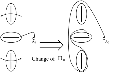
Figure 2: The change of $\Pi_{0}$ under the $a_{1}\to e^{2\pi i}a_{1}$

Finally, we will consider the transformation, $a_{1}\to e^{2\pi i}a_{1}$(see Fig2). Under this transformation $\Pi_{0},\Pi_{1}$ change respectively by

$$\Delta\Pi_{0}=2\left(2S_{1}\right),\qquad\Delta\Pi_{1}=2\left(S_{0}+S_{1}\right).$$ (4.5)

Collecting these results, we have the following monodromy contributions.

$$\Pi_{0} = \frac{W(\Lambda_{0})-W(0)}{\pi i}-\frac{1}{\pi i}\left(S_{0}+2S_{1}\right)\log\Lambda_{0}$$

$$+\frac{S_{0}}{2\pi i}\log\frac{S_{0}}{2W^{\prime\prime}(0)}+\frac{4}{2\pi i}S_{1}\log a_{1}+\cdots,$$

$$\Pi_{1} = \frac{W(i\Lambda_{0})-W(ia_{1})}{\pi i}-\frac{1}{\pi i}\left(S_{0}+2S_{1}\right)\log\Lambda_{0}$$ (4.6)

$$+\frac{S_{1}}{2\pi i}\log\frac{S_{1}}{2W^{\prime\prime}(ia_{1})}+\frac{2}{2\pi i}\left(S_{0}+S_{1}\right)\log a_{1}+\cdots.$$

Plugging these terms into (2.21), we obtain the effective superpotential, which is derived from naive integrating in [11][12].

4.2 Effective Superpotential

In the previous section, we obtained the logarismic contribution of the dual periods $\Pi_{i}$’s from the monodromy analysis. In this subsection we will compute the remaining terms. The explicit computation of $\Pi_{0}$ and $\Pi_{1}$ can be found in Appendix A up to the 4th order in $S_{i}$.

$$-\pi i\Pi_{0} = -W(\Lambda_{0})+W(0)-\left(S_{0}+2S_{1}\right)\log\Lambda_{0}$$ (4.7)

$$+\frac{S_{0}}{2}\log\frac{S_{0}}{2W^{\prime\prime}(0)}+2S_{1}\log a_{1}$$

$$+ga_{1}^{4}\Bigg{[}-2\left(x+y\right)\log\left(\frac{\Lambda_{0}}{a_{1}}\right)+x(\log x-1)$$

$$+4xy-\frac{3}{2}x^{2}-\frac{1}{2}y^{2}+\frac{9}{2}x^{3}-21x^{2}y+9xy^{2}-\frac{1}{2}y^{3}$$

$$-\frac{45}{2}x^{4}+\frac{466}{3}x^{3}y+\frac{76}{3}xy^{3}-131x^{2}y^{2}-\frac{5}{6}y^{4}\Bigg{]}+\cdots,$$

$$-\pi i\Pi_{1} = -W(i\Lambda_{0})+W(ia_{1})-\left(S_{0}+2S_{1}\right)\log\Lambda_{0}$$ (4.8)

$$+\frac{S_{1}}{2}\log\frac{S_{1}}{2W^{\prime\prime}(ia_{1})}+2\left(S_{0}+S_{1}\right)\log a_{1}$$

$$+ga_{1}^{4}\Bigg{[}-2(x+y)\log\left(\frac{\Lambda_{0}}{a_{1}}\right)+\frac{y}{2}\left(\log y-1\right)$$

$$+2x^{2}-xy-7x^{3}+9x^{2}y-\frac{6}{4}xy^{2}$$

$$+\frac{233}{6}x^{4}-\frac{262}{3}x^{3}y+\frac{152}{4}x^{2}y^{2}-\frac{10}{3}xy^{3}\Bigg{]}+\cdots,$$

where $x\equiv S_{0}/2ga_{1}^{4}$ , $y\equiv S_{1}/ga_{1}^{4}$. In this expression, the cut off $\Lambda_{0}$ is combined with the bare coupling $\alpha$ to form the gauge theory scale $\Lambda$ of the underlying $\mathcal{N}=2$ Yang-Mills theory [12][17].

The effective superpotential is given by (2.21). Since the exact low energy superpotential is obtained by integrating out the glueball superfields $S_{0},S_{1}$, we need to solve the equations $\partial W_{{\rm eff}}/\partial x=0\ ,\ \partial W_{{\rm eff}}/\partial y=0$. In the leading order, these equations are solved as,

$$x=T^{\frac{N_{1}}{2}},\qquad y=T^{\frac{N_{0}}{2}-1},\qquad T\equiv\left(\frac{\Lambda}{a_{1}}\right)^{\frac{4(N_{0}+2N_{1}-2)}{N_{1}(N_{0}-2)}}.$$ (4.9)

Using $T$ as the expansion parameter, the low energy superpotential $W_{\mathrm{low}}$ can be evaluated. Now we will compute some examples that correspond to the examples in the previous section.

$\mathbf{SO(6)\to SO(4)\times U(1)}$

As the first example, we consider the case $SO(6)\to SO(4)\times U(1)$. This gauge theory is realized by taking values as, $N_{0}=4\ ,\ N_{1}=1$ and $T=\frac{g^{2}\Lambda^{4}}{m^{2}}\equiv t^{2}$ The effective superpotential is obtained by plugging these values into the expression (2.21).

$$W_{\mathrm{low}}=\frac{m^{2}}{g}\left[-\frac{1}{2}+2T+\mathcal{O}(T^{5})\right].$$ (4.10)

In the calculation of this low-energy superpotential, some miraculous cancellation happens and this superpotential coincides with the confining phase superpotential (3.28). Thus the large $N$ duality is proved for this case up to the order ${\cal O}(T^{5})$ .

Case 2: Splitting of ${\bf SO(8)}$

As a next example, we will consider the case which corresponds to the splitting of the gauge group $SO(8)$. In this case, we consider the superpotentials generated by the fluxes of $N=N_{0}+2N_{1}=8$ D5-branes and a $O^{-}$-plane. To compare with the results of gauge theory, we will consider the following two breaking patterns.

$\mathbf{SO(8)\to SO(6)\times U(1)}$

First, we consider the case $SO(8)\to SO(6)\times U(1)$. This breaking is realized by choosing $N_{0}=6\ ,\ N_{1}=1$ and $T=t^{\frac{3}{2}}$. Thus effective superpotential is given by,

$$W_{\mathrm{low}}=\frac{m^{2}}{g}\left[-\frac{1}{2}+4T+2T^{2}-2T^{3}+4T^{4}+\mathcal{O}(T^{5})\right].$$ (4.11)

This superpotential coincides with the exact superpotential (3.37) in the gauge theory analysis up to ${\cal O}(T^{5})$.

$\mathbf{SO(8)\to SO(4)\times U(2)}$

As another splitting, we consider the case $SO(8)\to SO(4)\times U(2)$. This breaking corresponds to the case $N_{0}=4\ ,\ N_{1}=2$ and $T=t^{\frac{3}{2}}$. Thus effective superpotential is

$$W_{\mathrm{low}}=\frac{m^{2}}{g}\left[-1+4T^{2}-8T^{4}+64T^{6}-768T^{8}+\mathcal{O}(T^{10})\right].$$ (4.12)

This superpotential also coincides with the confining phase superpotential (3.39). Thus we examined the large $N$ duality for both of the breaking patterns in the gauge theory.

Case 3: $\mathbf{Sp(4)\to Sp(2)\times U(1)}$

Finally we consider a example of $Sp$ gauge theory. In this case, we have to choose the plus sign in (2.19) and set $N_{0}=2,N_{1}=1$. The low-energy superpotential is

$$W_{\mathrm{low}}=-\frac{m^{2}}{g}\left[-\frac{1}{2}+4T+2T^{2}-2T^{3}+4T^{4}+\mathcal{O}(T^{5})\right].$$ (4.13)

This superpotential coincides with the confining phase superpotential (3.46) Thus we examined the large $N$ duality for $Sp(2N)$ gauge theory.

Acknowledgements

The authors thank to Norisuke Sakai for reading this manuscript and giving us useful comments. The authors are obliged especially to Katsushi Ito for stimulus discussions and useful suggestions. Y.O. would like to thank M.Eto for continuous encouragement. H.F. is supported by JSPS research fellowship for young scientists.

Appendix A   Computation of Periods

In this appendix we will show the explicit computation of the periods $\Pi_{0},\Pi_{1}$ in (2.21). As discussed in section 2, the effective one-form is written as follows,

$$2dx\sqrt{W^{\prime 2}(x)+f_{2}(x)}=2dxg\sqrt{(x^{2}-{0^{+}}^{2})(x^{2}+x_{1}^{2})(x^{2}+x_{2}^{2})}.$$ (A.1)

Comparing the coefficient of $x^{3}$ on both sides in the above equation, we obtain the following relation.

$$\frac{m}{g}=\frac{1}{2}\left(-\Delta_{0}^{2}+x_{1}^{2}+x_{2}^{2}\right)=a_{1}^{2}.$$ (A.2)

Here we define new variables given by,

$$\Delta_{0}\equiv 0^{+}=-0^{-},\qquad\Delta_{1}\equiv\frac{1}{2}(x_{2}-x_{1}),$$ (A.3)

$$Q\equiv\frac{1}{2}(x_{2}+x_{1}),\quad w\equiv\frac{\Delta_{0}}{Q},\ \ u\equiv\frac{\Delta_{1}}{Q}.$$ (A.4)

Since $f_{2}$ is considered as a small perturbation, $\Delta_{0}$, $\Delta_{1}$ and $Q$ satisfy

$$|\Delta_{0}|\sim|\Delta_{1}|\ll|Q|.$$ (A.5)

Under this relation, we can expand the periods $S_{0}$ and $S_{1}$ in powers of $w$ and $u$.

$$S_{0} = \frac{g}{\pi i}\int_{-\Delta_{0}}^{\Delta_{0}}\sqrt{(x^{2}-\Delta_{0}^{2})(x^{2}+x_{1}^{2})(x^{2}+x_{2}^{2})}\ dx$$ (A.6)

$$= \frac{g}{2}Q^{2}w^{2}\left[1-u^{2}+\frac{w^{2}}{4}+\frac{w^{2}u^{2}}{2}+\frac{w^{2}u^{4}}{2}-\frac{u^{2}w^{4}}{4}+\mathcal{O}\left((uw)^{7}\right)\right],$$

$$S_{1} = \frac{g}{\pi i}\int_{x_{1}}^{x_{2}}\sqrt{(x^{2}-\Delta_{0}^{2})(x^{2}+x_{1}^{2})(x^{2}+x_{2}^{2})}\ dx$$ (A.7)

$$= gQ^{4}u^{2}\left[1+\frac{1}{2}w^{2}-\frac{1}{8}w^{4}-\frac{1}{8}w^{4}u^{2}+\frac{1}{16}w^{6}+\mathcal{O}\left((uw)^{7}\right)\right].$$

Next we will compute the dual periods $\Pi_{i}$’s. In the computation, we will discard any contributions of ${\cal O}(\Lambda_{0}^{-1})$, since $\Lambda_{0}$ is introduced as cut-off of infinite volume of dual three cycles.

$$\frac{\pi i}{g}\Pi_{0} = \int_{\Delta_{0}}^{\Lambda_{0}}\sqrt{(x^{2}-\Delta_{0}^{2})(x^{2}+x_{1}^{2})(x^{2}+x_{2}^{2})}\ dx$$ (A.8)

$$= \frac{1}{4}(\Lambda_{0})^{4}+\frac{1}{2}(\Lambda_{0})^{2}Q^{2}\left(1+u^{2}-\frac{1}{2}w^{2}\right)$$

$$-Q^{4}\log(2\Lambda_{0})\left(\frac{w^{2}}{2}+\frac{w^{2}u^{2}}{2}+\frac{w^{4}}{8}+2u^{2}\right)$$

$$+\frac{Q^{4}}{32}w^{4}-\frac{Q^{4}w^{2}}{4}\left(1+u^{2}\right)+\sum_{n=2}^{\infty}c_{n}\frac{(-1)^{n-2}}{(n-2)!}(4Q^{2}u)^{n}G^{(n-2)}(a)\Bigg{|}_{a=0}$$

where $c_{n}$ are the coefficient of the power expansion of $\sqrt{1+x}$. The computation for $\Pi_{1}$ is obtained in a similar way.

$$\frac{\pi i}{g}\Pi_{1} = \int_{x_{2}}^{\Lambda_{0}}\sqrt{(x^{2}+\Delta_{0}^{2})(x^{2}+x_{1}^{2})(x^{2}+x_{2}^{2})}dx$$ (A.9)

$$= \frac{\Lambda_{0}^{6}}{4}+\Lambda_{0}^{3}Q^{2}\left(-\frac{1+u^{2}}{2}+\frac{w^{2}}{4}\right)+Q^{4}\log(4\Lambda^{3})\left(-u^{2}-\frac{(1+u^{2})w^{2}}{4}\right)$$

$$- Q^{4}\frac{(1+u^{2})w^{2}}{4}+Q^{4}\left(u^{2}+\frac{w^{2}(1+u^{2})}{4}\right)\log(4Q^{2}u^{2})+Q^{4}\frac{1+u^{4}}{4}$$

$$- \frac{1}{2}\sum_{n=1}^{\infty}c_{n}(-1)^{(n)}\frac{w^{2n}Q^{2n}}{(n-1)!}H^{(n-1)}(a)\Bigg{|}_{a=0}.$$

In the above expansion, we used the following generating functions

$$G(a) \equiv -\sqrt{\frac{x_{1}^{2}+\Delta_{0}^{2}+a}{x_{1}^{2}+a}}\log\left(\sqrt{x_{1}^{2}+\Delta_{0}^{2}+a}+\sqrt{x_{1}^{2}+a}-\log\Delta_{0}\right),$$

$$H(a) \equiv -a\left(\log(4\Lambda_{0}^{3})-\log(4Q^{2}u)\right)$$

$$+\sqrt{(x_{1}^{2}+a)(x_{2}^{2}+a)}\log\Bigg{(}(\Lambda_{0}^{3}+a)(x_{1}^{2}-x_{2}^{2})/\{-(x_{1}^{2}+x_{2}^{2}+2a)(\Lambda_{0}^{3}+a)$$

$$+2(x_{1}^{2}+a)(x_{2}^{2}+a)+2\sqrt{(x_{1}^{2}+a)(x_{2}^{2}+a)(\Lambda_{0}^{3}-x_{1}^{2})(\Lambda_{0}^{3}-x_{2}^{2})}\}\Bigg{)}.$$

The dual periods $\Pi_{0}$ and $\Pi_{1}$ are expressed in terms of the periods $S_{0}$ and $S_{1}$ by comparing order by order in $w$ and $u$ in the expressions (A.7)$\sim$(A.9).

$$-\pi i\Pi_{0} = -W(\Lambda_{0})+W(0)-\left(S_{0}+2S_{1}\right)\log\Lambda_{0}+\frac{S_{0}}{2}\log\frac{S_{0}}{2W^{\prime\prime}(0)}+2S_{1}\log a_{1}-\frac{S_{0}}{2}$$ (A.10)

$$+\frac{1}{4ga_{1}^{4}}\left(8S_{0}S_{1}-\frac{3}{2}S_{0}^{2}-2S_{1}^{2}\right)+\frac{1}{8(ga_{1}^{4})^{2}}\left(\frac{9}{2}S_{0}^{3}-42S_{0}^{2}S_{1}+36S_{0}S_{1}^{2}-4S_{1}^{3}\right)$$

$$+\frac{1}{16(ga_{1}^{4})^{3}}\left(-\frac{45}{2}S_{0}^{4}+\frac{932}{3}S_{0}^{3}S_{1}+\frac{608}{3}S_{0}S_{1}^{3}-524S_{0}^{2}S_{1}^{2}-\frac{40}{3}S_{1}^{4}\right)$$

$$+\cdots,$$

$$-\pi i\Pi_{1} = -W(i\Lambda_{0})+W(ia_{1})-\left(S_{0}+2S_{1}\right)\log\frac{\Lambda_{0}}{a_{1}}-S_{1}\log a_{1}+\frac{S_{1}}{2}\log\frac{S_{1}}{m}-\frac{S_{1}}{2}$$ (A.11)

$$+\frac{1}{4ga_{1}^{4}}\left(2S_{0}^{2}-2S_{0}S_{1}\right)+\frac{1}{8(ga_{1}^{4})^{2}}\left(-7S_{0}^{3}+18S_{0}^{2}S_{1}-6S_{0}S_{1}^{2}\right)$$

$$+\frac{1}{16(ga_{1}^{4})^{3}}\left(\frac{233}{6}S_{0}^{4}-\frac{524}{3}S_{0}^{3}S_{1}+152S_{0}^{2}S_{1}^{2}-\frac{80}{3}S_{0}S_{3}^{3}\right)+\cdots.$$

References

- [1] G.’t Hooft, “A Planar Diagram Theory For Strong Interactions”, Nucl. Phys. B72 (1974) 461.
- [2] J.Maldacena, “The Large N Limit of Superconformal Field Theories and Supergravity”, Adv. Theor. Math. Phys. 2 (1998) 231. Int. J.Theor. Phys. 38 (1999) 1113 [hep-th/9711200]. S.S.Gubser, I.R.Klebanov and A.M.Polyakov, “Gauge Theory Correlators from Non-Critical String Theory”, Phys. Lett. B428 (1998) 105 [hep-th/9802109]. E.Witten, “Anti de Sitter Space and Holography”, Adv. Theor. Amth. Phys. 2 (1998) 505 [hep-th/9802150].
- [3] I.R.Klebanov and E.Witten, “Superconformal Field Theory on Threebranes at a Calabi-Yau Singularity”, Nucl. Phys. B536 (1998) 199 [hep-th/9807080].
- [4] I.R.Klebanov and N.A.Nekrasov, “Gravity Duals of Fractional Branes and Logarithmic RG Flow”, Nucl. Phys. B574 (2000) 263 [hep-th/9911096]. I.R.Klebanov and A.A.Tseytlin, “Gravity Duals of Supersymmetric SU(N) x SU(N+M) Gauge Theories”, Nucl. Phys. B578 (2000) 123 [hep-th/0002159]. I.R.Klebanov and M.J.Strassler, “Supergravity and a Confining Gauge Theory: Duality Cascades and SB-Resolution of Naked Singularities”, JHEP 0008 (2000) 052 [hep-th/000719].
- [5] R.Gopakumar and C.Vafa, “Topological Gravity as Large N Topological Gauge Theory”, Adv. Theor. Math. Phys. 2 (1998) 413 [hep-th/9802016]. R.Gopakumar and C.Vafa, “On the Gauge Theory/Geometry Correspondence”, Adv. Theor. Math. Phys. 3 (1999) 1415 [hep-th/9811131]. R.Gopakumar and C.Vafa, “M-Theory and Topological Strings-I”,[hep-th/9809187]. “M-Theory and Topological Strings-II”, [hep-th/9812127]. H.Ooguri and C.Vafa, “Knot Invariants and Topological Strings”, Nucl. Phys. B577 (2000) 419 [hep-th/9912123]. H.Ooguri and C.Vafa, “Worldsheet Derivation of a Large N Duality”, [hep-th/0205297].
- [6] C.Vafa , “Superstrings and Topological Strings at Large N,” J. Math. Phys. 42 (2001) 2798 [hep-th/0008142].
- [7] M.Atiyah, J.Maldacena and C.Vafa, “An M-theory Flop as a Large N Duality”, [hep-th/0011256].
- [8] M.Atiyah and E.Witten, “M-Theory Dynamics On A Manifold Of Holonomy”, [hep-th/0107177]. H.Ita, Y.Oz and T.Sakai, “Comments on M Theory Dynamics on G2 Holonomy Manifolds ”, JHEP 0204 (2002) 001 [hep-th/0203052]. T.Friedmann, “On the Quantum Moduli Space of M Theory Compactifications”, Nucl.Phys. B635 (2002) 214-224 [hep-th/0203256].
- [9] M.Aganagic, A.Klemm and C.Vafa, “Disk Instantons, Mirror Symmetry and the Duality Web”, Z.Naturforsch. A57 (2002) 1 [hep-th/0105045].
- [10] Taylor and C.Vafa, “RR Flux on Calabi-Yau and Partial Supersymmetry Breaking”, Phys. Lett. B474 (2000) 130 [hep-th/9912152].
- [11] G.Veneziano and S.Yankielowicz, “An Effective Lagrangian for the pure Supersymmetric Yang-Mills Theory”, Phys. Lett. B113 (1982) 321, T.R.Taylor, G.Veneziano and S.Yankielowicz, “Supersymmetric QCD and its Massless Limit :An Effective Lagrangian Analysis”, Nucl.Phys.B218 (1983) 493.
- [12] F.Cachazo, K.Intriligator and C.Vafa, “A Large Duality via Geometric Transition”, Nucl. Phys. B603 (2001) 3 [hep-th/0103067].
- [13] F.Cachazo, S.Katz and C.Vafa, “Geometric Transitions and N=1 Quiver Theories”, [hep-th/0108120]. F.Cachazo, B.Fiol, K.Intriligator S.Katz and C.Vafa, “A Geometric Unification of Dualities”, Nucl. Phys. B628 (2002) 3 [hep-th/0110028]. B.Fiol, “Duality Cascades and Duality Walls”, [hep-th/0205155].
- [14] K.Dasgupta, K.Oh and R.Tatar “Geometric Transition, Large N Dualities and MQCD Dynamics”, Nucl.Phys. B610 (2001) 331-346, [hep-th/0105066]; “Open/Closed String Dualities and Seiberg Duality from Geometric Transitions in M-theory”, [hep-th/0106040]. K.Dasgupta, K.Oh, J.Park and R.Tatar, “Geometric Transition versus Cascading Solution”, JHEP 0201 (2002) 031, [hep-th/0110050]. K.Oh and R.Tatar, “Duality and Confinement in N=1 Supersymmetric Theories from Geometric Transitions”, [hep-th/0112040]; “Renormalization Group Flows on D3 branes at an Orbifolded Conifold”, JHEP 0005 (2000) 030, [hep-th/0003183].
- [15] S.Sinha and C.Vafa, “ and Chern-Simons at Large N”, [hep-th/0012136].
- [16] B.Acharya, M.Aganagic, K.Hori and C.Vafa, “Orientifolds, Mirror Symmetry and Superpotentials”, [hep-th/0202208].
- [17] J.D.Edelstein, K.Oh and R.Tatar, “Orientifold, Geometric Transition and Large N Duality for Gauge Theories”, JHEP 0105 (2001) 009 [hep-th/0104037].
- [18] S.Imai and T.Yokono, “Comments on orientifold projection in the conifold and SO x USp duality cascade”, Phys. Rev. D65 (2002) 066007 [hep-th/0110209].
- [19] J.Gomis, “On SUSY Breaking And SB From String Duals”, Nucl.Phys. B624 (2002) 181, [hep-th/0111060].
- [20] S.Kachru, S.Katz, A.Lawrence, J.McGreevy, “Open string instantons and superpotentials”, Phys.Rev.D62 (2000) 026001 [hep-th/9912151]. “Mirror symmetry for open strings”, [hep-th/0006047]. I.Brunner, M.R.Douglas, A.Lawrence and C.Romelsberger “D-branes on the Quintic”, JHEP 0008 (2000) 015, [hep-th/9906200].
- [21] S.Elitzur, A.Forge, A.Giveon, K.Intriligator and E.Rabinovici, “Massless Monopoles Via Confining Phase Superpotentials”, Phys. Lett. B379 (1996) 121, [hep-th/9603051].
- [22] S.Terashima and S.-K.Yang, “Confining phase of N=1 supersymmetric gauge theories and N=2 massless solitons”, Phys. Lett. B391 (1997) 107 [hep-th/9607151]. S.Terashima and S.-K. Yang, “ADE confining phase superpotentials”, Nucl. Phys. B519 (1998) 453 [hep-th/9706076]. S.Terashima “Supersymmetric gauge theories with classical groups via M theory five-brane ”, Nucl. Phys. B526 (1998) 163 [hep-th/9712172].
- [23] P.Candelas and X.C.de la Ossa “Comments on Conifold”, Nucl.Phys.B342 (1990) 246.
- [24] A.Strominger, “Massless Black Holes and Conifolds in String Theory”, Nucl. Phys. B451 (1995) 96 [hep-th/9504090].
- [25] I.Antoniadis, H.Partouche and T.R.Taylor, “Spontaneous Breaking of N=2 Global Supersymmetry”, Phys. Lett. B372 (1996) 83 [hep-th/9512006]. S.Ferrara, L.Girardello and M.Porrati “Spontaneous Breaking of N=2 to N=1 in Rigid and Local Supersymmetric Theories”, Phys. Lett. B376 (1996) 275 [hep-th/9512180]. I.Antoniadis and T.R.Taylor, “Dual N=2 SUSY Breaking”, Fortsch. Phys. 44 (1996) 487 [hep-th/9604062].
- [26] S.Gukov, C.Vafa and E.Witten “CFT’s From Calabi-Yau Four-folds”, Nucl.Phys. B584 (2000) 69-108, [hep-th/9906070]. S.Gukov, “Solitons, Superpotentials and Calibrations”, Phys.Lett. B474 (2000) 130-137, [hep-th/9911011].
- [27] N.Seiberg and E.Witten, “Monopole Condensation, And Confinement In N=2 Supersymmetric Yang-Mills Theory”, Nucl. Phys. B426 (1994) 19 [hep-th/9407087].
- [28] R.G.Leigh and M.J.Strassler, “Duality of Sp(2N(c)) and SO(N(c)) supersymmetric gauge theories with adjoint matter”, Phys. Lett. B356 (1995) 492 [hep-th/9505088].
- [29] P.C.Argyres and A.D.Shapere, “The Vacuum Structure of N=2 SuperQCD with Classical Gauge Groups”, Nucl. Phys. B461 (1996) 437 [hep-th/9509175].
- [30] U.H.Danielsson and B.Sundborg, “The Moduli space and monodromies of supersymmetric Yang-Mills Theory”, Phys. Lett. B358 (1995) 273 [hep-th/95044102]. A.Brandhuber and K.Landsteiner, “On the monodromies of N=2 supersymmetric Yang-Mills theory with ”, Phys. Lett. B358 (1995) 73 [hep-th/9507008].
- [31] C.Ahn, “Confining Phase of Gauge Theories via M Theory Fivebrane”, Phys. Lett. B426 (1998) 306 [hep-th/9712149].
- [32] C.Ahn, K.Oh and R.Tatar “M Theory Fivebrane and Confining Phase of Gauge Theories”, J.Geom. Phys. 28 (1998) 163 [hep-th/9712005].
- [33] M.R.Douglas and S.H.Shenker, “Dynamics of Supersymmetric Gauge Theory”, Nucl. Phys. B447 (1995) 271 [hep-th/9503163].