hep-th/0205299

Exact Solutions and the Cosmological Constant Problem in Dilatonic-Domain-Wall Higher-Curvature String Gravity

Nick E. Mavromatos
Department of Physics, Theoretical Physics, King’s College London,
Strand, London WC2R 2LS, United Kingdom.

and

John Rizos
Department of Physics, University of Ioannina,
GR 45100 Ioannina, Greece,

Abstract

In this article we extend previous work by the authors, and elaborate further on the structure of the general solution to the graviton and dilaton equations of motion in brane world scenaria, in the context of five-dimensional effective actions with ${\cal O}(\alpha^{\prime})$ higher-curvature corrections, compatible with bulk string-amplitude calculations. We consider (multi)brane scenaria, dividing the bulk space into regions, in which one matches two classes of general solutions, a linear Randall-Sundrum solution and a (logarithmic) dilatonic domain wall (bulk naked singularity). We pay particular attention to examining the possibility of resolving the mass hierarchy problem together with the vanishing of the vacuum energy on the observable world, which is taken to be a positive tension brane. The appearance of naked dilatonic domain walls provides a dynamical restriction of the bulk space time. Of particular interest is a dilatonic-wall solution, which after appropriate coordinate transformation, results in a linear dilaton conformal field theory. The latter may provide a holographic resolution of the naked singularity problem. All the string-inspired models involved have the generic feature that the brane tensions are proportional to the string coupling $g_{s}$; it remains a challenge for string theory, therefore, to show whether microscopic models respecting this feature can be constructed.

May 2002

1 Introduction

Randall and Sundrum [1] (RS) have proposed a new solution to the mass hierarchy problem on the observable world by means of gravitational interactions in the bulk coordinate of a five-dimensional space time, in which our world is viewed as an embedded three-brane domain wall. The scenario involves a hidden world, represented by a second parallel brane, whose separation from the first determines the mass hierarchy on the observable world. A necessary ingredient in the above construction is an orbifold in the bulk direction, which restricts the bulk space onto that between the branes. This set-up is implemented by the following non-factorizable form of the metric:

$$ds^{2}=e^{-2\sigma(z)}\eta_{ij}dX^{i}dX^{j}+dz^{2}~{},i,j=0,1,\dots 3$$ (1)

This is a solution to the standard Einstein equations provided one chooses the following form of the metric function $\sigma(z)$, in the simplest case of a constant dilaton $\Phi$: $\sigma(z)=\sum_{i}{k}\left|z-z_{i}\right|$, with $i$ denoting the $i-th$ brane, located at $z_{i}$ along the bulk direction. This metric is known in the literature as the Randall-Sundrum (RS) metric [1].

In a recent article [2], we have considered five-dimensional actions including ${\cal O}(\alpha^{\prime})$ higher-curvature corrections, compatible with string-amplitude computations [3], with non-constant (bulk-coordinate dependent) dilaton fields, where $\alpha^{\prime}=M_{s}^{-2}$ is the Regge slope of the string, and $M_{s}$ the string mass scale. Such corrections, but for constant dilaton fields or for actions that are not derived from string amplitudes, had been considered earlier in [4, 5], with different conclusions from ours.

The appearance of quadratic (Gauss-Bonnet type) terms in the effective action, may occur in Heterotic M-theory scenaria of Horava-Witten type [6], which are known to have D-branes. In type IIB string theories on the other hand, which are also known to to admit D-brane solutions, there are no quadratic Gauss-Bonnet corrections at tree level, although such terms may be generated through loop corrections. The presence of higher-curvature terms in the effective action leads to interesting physics, and a lot of works have appeared recently examining potential physical applications in a variety of context, ranging from static solutions to cosmology [7, 8, 9]. Moreover, in standard string theory, it is known that higher-curvature corrections lead to highly non-trivial results, for instance new types of Black-Hole solutions with (secondary) dilaton hair [10], or singularity-free cosmologies [11].

In view of this wide range of applications, we therefore feel that it is appropriate to present a systematic analysis of the general structure of the solutions of the string-effective action to ${\cal O}(\alpha^{\prime})$, which extends and completes the analysis of [2]. In this article we elaborate further on the structure of the general solution to the equations of motion, and discuss physical applications, especially from the point of view of resolving simultaneously the mass hierarchy problem, the positivity of the tension of our observable brane world, and the vanishing of the total vacuum energy induced on our world.

In particular, we examine two classes of solutions, a linear Randall-Sundrum solution, with constant dilaton, and a logarithmic domain-wall solution, where the bulk dependent dilaton and the metric have bulk naked singularities. The article deals with a discussion on the integrability conditions of such singularities, as well as a detailed matching of these classes of solutions in various scenaria, where brane junctions separate the bulk space into regions. The presence of dilatonic domain walls implies a dynamical restriction of the bulk space.

The structure of the article is as follows: In section 2 we review the general solution of [2] to the graviton and dilaton equations of motion, including the string-inspired Gauss-Bonnet quadratic curvature contributions and dilaton four-derivative terms in the gravitational action. In section 3 we discuss effective quantities, such as Planck mass and Vacuum energy, as measured by a four-dimensional observer, living on the observable brane world. In section 4 we discuss the structure of two types of exact solutions. One type is the Linear RS solution [1], while the other is a dilatonic domain wall (bulk logarithmic naked singularity). We discuss integrability conditions of these latter naked singularities in the bulk space, to which we restrict ourselves throughout this work. We show how such integrable singularities are consistent solutions of the ${\cal O}(\alpha^{\prime})$ equations of motion. In section 5 we discuss matching of these two types of exact solutions at various brane junctions, separating the bulk space into regions. We commence our analysis by discussing singe brane scenaria and their disadvantages from a physical point of view. We then proceed to analyze multibrane scenaria which can solve the mass hierarchy problem on a positive tension observable world simultaneously with a vanishing vacuum energy (cosmological constant) on the brane. In section 6 we discuss a possible resolution of the bulk naked singularity problem by means of holography induced by a linear-dilaton domain-wall solution, which, as we show, is a specific case of the general solution of [2]. Finally, in section 7 we present our conclusions and outlook.

2 General Solution with Gauss-Bonnet Interactions: a Review

In this section we review the general solution of the ${\cal O}(\alpha^{\prime})$ string-inspired effective action, in the five-dimensional effective case, discussed in detail in [2]. We consider the action:

$$S=S_{5}+S_{4}$$ (2)

where $S_{5}$:

$$S_{5} = \int d^{5}x\sqrt{-g}\left[-R-\frac{4}{3}\left(\nabla_{\mu}\Phi\right)^{2}+f(\Phi)\left(R^{2}-4R_{\mu\nu}^{2}+R_{\mu\nu\rho\sigma}^{2}\right)\right.$$ (3)

$$+\xi(z)e^{\zeta\Phi}+\left.c_{2}~{}f(\Phi)\left(\nabla_{\mu}\Phi\right)^{4}+\dots\right]$$

with $\Phi$ the dilaton field, and the $\dots$ denoting other types of contraction of the four-derivative dilaton terms which will not be of interest to us here, given that by appropriate field redefinitions, leaving the string amplitudes invariant [3], one can always cast such terms in the above form.

The four-dimensional part $S_{4}$ of the action (2) is defined as:

$$S_{4}=\sum_{i}\int d^{4}x\sqrt{-g_{(4)}}e^{\omega\Phi}v(z_{i})$$ (4)

where

$$g_{(4)}^{\mu\nu}=\left\{\begin{array}[]{l}g^{\mu\nu}\ ,\,\mu,\nu<5\\ 0\ \ \ ,\ \mbox{otherwise}\\ \end{array}\right.$$ (7)

and the sum over $i$ extends over D-brane walls located at $z=z_{i}$ along the fifth dimension.

The above action is compatible with closed string amplitude computations in the five-dimensional space times [3]. In our opinion, such a compatibility is not only natural, but also necessary in view of the assumption of closed string propagation in the bulk. In the stringy case one has [2]:

$$~{}~{}f(\Phi)=\lambda~{}e^{\theta\Phi}~{},~{}\lambda=\alpha^{\prime}/8g_{s}^{2}>0~{},~{}c_{2}=\frac{16}{9}\frac{D-4}{D-2}$$ (8)

$$\zeta=-\theta=\frac{4}{\sqrt{3(D-2)}}~{}~{}(=4/3~{}~{}{\rm for}~{}~{}D=5)$$

where $g_{s}$ is the string coupling and $D$ is the number of space-time dimensions. In this work we shall restrict ourselves to the case $D=5$ [2]. However, for reasons that will be clarified below, we shall keep the coefficient $c_{2}$ of the dilaton quartic terms in the action general. As we shall see, our results do not depend crucially on its value.

In this case, the equations of motion for the graviton and dilaton fields obtained from (2) read respectively:

$$0=R^{\mu\nu}+\frac{1}{2}g^{\mu\nu}\left(-R-\frac{4}{3}(\nabla\Phi)^{2}+c_{2}f(\Phi)(\nabla\Phi)^{4}+\xi(z)e^{\zeta\Phi}\right)$$ (9)

$$+\frac{1}{2}\sum_{i}{\frac{\sqrt{-g_{(4)}}}{\sqrt{-g}}}g_{(4)}^{\mu\nu}e^{\omega\Phi}v(z_{i})+\frac{4}{3}(\nabla^{\mu}\Phi)(\nabla^{\nu}\Phi)$$

$$-f(\Phi)\left(2\alpha RR^{\mu\nu}+2\beta{R^{\mu}}_{\sigma}R^{\nu\sigma}+2\gamma R^{\mu}_{\sigma\tau\rho}R^{\nu\sigma\tau\rho}\right)$$

$$+\frac{1}{2}g^{\mu\nu}f(\Phi)\left(\alpha R^{2}+\beta R_{\sigma\tau}R^{\sigma\tau}+\gamma R_{\sigma\tau\rho{k}}R^{\sigma\tau\rho{k}}\right)$$

$$+2\alpha\{{(g^{\mu\nu}f(\Phi)R)_{;\sigma}}^{\sigma}-(f(\Phi)R)_{;}^{\mu\nu}\}$$

$$+\beta\{(g^{\mu\nu}f(\Phi)R^{\sigma\tau})_{;\sigma\tau}+{(f(\Phi)R^{\mu\nu})_{;\sigma}}^{\sigma}-{{(f(\Phi)R^{\mu\sigma})_{;}}^{\nu}}_{\sigma}-{{(f(\Phi)R^{\nu\sigma})_{;}}^{\mu}}_{\sigma}\}$$

$$+2\gamma\{(f(\Phi)R^{\mu\sigma\nu\tau})_{;\sigma\tau}+(f(\Phi)R^{\mu\sigma\nu\tau})_{;\tau\sigma}\}$$

$$-2c_{2}f(\Phi)(\nabla^{\mu}\Phi)(\nabla^{\nu}\Phi){(\nabla\Phi)}^{2}$$

and

$$0=\frac{8}{3}\nabla^{2}\Phi+f^{\prime}(\phi)\left(\alpha R^{2}+\beta R_{\mu\nu}R^{\mu\nu}+\gamma R_{\mu\nu\rho\sigma}R^{\mu\nu\rho\sigma}\right)+\zeta\xi(z)e^{\zeta\Phi}+$$ (10)

$$\sum_{i}{\frac{\sqrt{-g_{(4)}}}{\sqrt{-g}}}\omega e^{\omega\Phi}v(z_{i})-4c_{2}\nabla_{\mu}\left(f(\Phi)(\nabla^{\mu}\Phi)(\nabla\Phi)^{2}\right)+c_{2}f^{\prime}(\Phi)\left(\nabla\Phi\right)^{4}$$

In the above formulæ  the symbol ; denotes covariant differentiation, and the prime denotes differentiation with respect to $\Phi$.

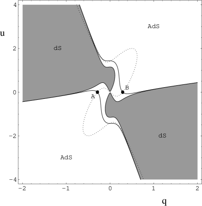
Figure 1: The phase-space of the general solution of the graviton-dilaton equations of motion in the presence of Gauss-Bonnet curvature-squared terms in the low-energy effective action. The regions where the bulk cosmological constant is negative (positive), and hence the space time is de Sitter (dS) (anti-de-Sitter (AdS)) are indicated. For detailed explanations we refer the reader to ref. [2]. The dashed lines indicate the exact logarithmic solution (24), while the dots at A and B denote the Randall-Sundrum (RS) solution (20). The continuous lines passing through A and B represent the solution of [2] interpolating between the RS solution near our brane world and a bulk naked singularity at infinity. The integrability conditions on the naked singularities impose further restrictions on the solutions phase space to be discussed in the current article.

The general solution has been studied in detail in [2]. It has been shown there that among the solutions there is one which interpolates continuously between an RS type of solution (1), occurring at $z=+\infty$, and a naked singularity at $z=0$, which is however integrable. This solution is important in that it implies the dynamical formation of domain walls in the bulk direction, however the relevant distance from the singularity is infinite, and hence it cannot provide a solution to the hierarchy problem à la Randall-Sundrum [1]. Graphically, the phase space of the solution is depicted in figure 1.

The implementation of bulk naked singularities, or equivalently dilatonic domain walls as they are called in the literature [12, 13, 14, 15, 16], due to the fact that both dilaton and graviton fields exhibit logarithmic singularities, has been connected to a possible resolution of the cosmological constant problem in the context of lowest-order brane-world Einstein gravity [12, 13]. The idea is that the vacuum energy of the brane world curves the fifth dimension, leaving a flat (Poincare invariant) four-dimensional brane world intact. However, as demonstrated in [15], such a scenario hides a fine-tuning in the following sense: one should resolve the naked singularity in a way consistent with classical equations of motion. This requires the brane world tension to be equal in magnitude and opposite in sign with the tension of a second brane (hidden world), placed at the singularity, whose presence is necessitated by the requirement of satisfaction of the equations of motion. In this way, the expectations of [13] for a self tuning mechanism for the cancellation of the cosmological constant do not work.

As discussed recently in [17], if one imposes supergravity in the bulk, then there are topological obstructions, associated with extra degrees of freedom of the supergravity multiplet, which force the naked singularity to lie beyond the second brane, and thus being shielded.

An additional problem with brane world scenaria is the fact that in the original RS model [1] the physical world was located on a brane with negative tension, which is a serious instability [18]. To tackle this problem, bigravity scenaria have been proposed [19], i.e. multibrane scenaria involving branes with alternating-sign tensions, in such a way that our world is identified with a positive tension brane surrounded by negative tension ones, lying asymmetrically from our world. Again such models have been studied in the context of the lowest-order Einstein gravity actions, and actually with constant dilaton fields in the bulk. Moreover the original orbifold construction of [1] has been imposed.

It is the purpose of this article to discuss all the above issues, when string-inspired ${\cal O}(\alpha^{\prime})$ higher-curvature corrections are taken into account, with non-trivial bulk dependence of the dilaton field, which, together with the graviton, is assumed propagating in the bulk. In particular, we shall demonstrate first that the original Randall-Sundrum scenario, with or without orbifold constructions, is capable of solving both the hierarchy, and the smallness of the cosmological constant on the brane world. We shall also discuss other scenaria involving dilatonic domain walls, specifically we shall discuss multibrane scenaria involving dilatonic brane worlds shielded by a number of ghost branes, surrounding our physical brane world. In such constructions we shall demonstrate the possibility of solving the mass hierarchy problem, on a positive tension observable brane world, simultaneously with the vanishing of the vacuum energy on the brane. To this end, we shall employ alternative solutions to the system of equations of motions (9),(10), that were also presented in [2], but not studied further there. Finally, we shall demonstrate the existence of a dilatonic-wall solution, which, under an appropriate bulk coordinate transformation, results in a linear dilaton background $\sigma$-model conformal field theory. Such a solution exhibits holographic properties, which may be used to provide a resolution of the bulk naked singularity problem. We shall analyze first the important rôle of the higher-curvature corrections in single brane scenaria, and discuss their physical disadvantages. Then we shall proceed to analyze the multibrane scenaria, and discuss their advantages over single brane models.

3 Four-Dimensional Effective Action

Observers on brane worlds will have to integrate over the coordinate $z$ in order to obtain the effective four-dimensional action. The integrated coefficients of the $R^{(4)}(x)$ terms yield contributions to the effective four-dimensional Planck Mass scale, $M_{P}$, whilst the rest of the terms contribute to the effective four-dimensional vacuum energy.

Using the warped five-dimensional metric in the form $ds^{2}=e^{-2\sigma(z)}\,g^{(4)}_{\mu\nu}(x)dx^{\mu}\,dx^{\nu}+dz^{2}$, where $\mu,\nu$ are four-dimensional space-time indices and $g_{\mu\nu}^{(4)}$ is a four-dimensional (brane) metric tensor, one obtains:

$$\sqrt{-g}\,R(x)=\sqrt{-g^{(4)}(x)}\,\left(e^{-2\sigma(z)}\,R^{(4)}(x)+e^{-4\sigma(z)}\,{\cal R}\right)$$ (11)

$$\lambda e^{-\frac{4}{3}\Phi(z)}\sqrt{-g}\,R_{GB}(x) = \sqrt{-g^{(4)}(x)}\,\lambda e^{-\frac{4}{3}\Phi(z)}\,\left(4\,e^{-2\sigma(z)}(3\sigma^{\prime}(z)^{2}-2\sigma^{\prime\prime}(z))\,R^{(4)}(x)\right.$$ (12)

$$\left.-2\,(R_{\mu\nu\rho\sigma}^{2}-R_{\mu\nu}^{2})+e^{-4\sigma(z)}\,{\cal R}_{GB}\right)$$

$$\sqrt{-g}\,(\nabla_{\mu}\Phi)^{2}=\sqrt{-g^{(4)}(x)}\,\left(e^{-4\sigma(z)}\,\Phi^{\prime}(z)^{2}+e^{-2\,\sigma(z)}\,(\nabla_{i}\Phi^{(4)}(x))^{2}\right)$$ (13)

where

$${\cal R} = 4\,(5\,\sigma^{\prime}(z)^{2}-2\,\sigma^{\prime\prime}(z))$$ (14)

$${\cal R}_{GB} = 24\,\left(5\,{{\sigma^{\prime}(z)}^{4}}-4\,{{\sigma^{\prime}(z)}^{2}}\,\sigma^{\prime\prime}(z)\right)$$ (15)

and the superscript $(4)$ denotes four-dimensional quantities, evaluated on the brane worlds.

The expression for the four-dimensional Planck’s constant $M_{P}$, as perceived by an observer living on the brane world located a finite $z$, is given by (c.f. (11),(12)):

$$M_{P}^{2}=M_{s}^{3}\int_{-\infty}^{\infty}dze^{-2\sigma(z)}\left(1-4~{}\lambda e^{-\frac{4}{3}\Phi(z)}(3(\sigma^{\prime}(z))^{2}-2\sigma^{\prime\prime}(z))\right)$$ (16)

where $M_{s}$ is the five-dimensional (bulk) string mass scale.

In this framework, the four-dimensional effective vacuum energy on the observable brane world $\Lambda_{\rm total}$ receives two kinds of contributions: (i) from the tension of the brane world we are living on, located, say, at $z=z_{i}$, $V_{\rm brane}(z_{i})\equiv e^{\omega\Phi(z_{i})}v(z_{i})$, and (ii) from the bulk terms in the action (2), that include the cosmological constant $\xi$, the dilaton derivative terms, as well as the ${\cal R}$, ${\cal R}_{GB}$ dependent terms in (11),(12). Therefore, the expression for the total four-dimensional vacuum energy reads:

$$\Lambda_{\rm total}(z_{i})=\Omega+V_{\rm brane}(z_{i})~{},$$ (17)

$$\Omega=\int_{-\infty}^{+\infty}dz\,e^{-4\sigma(z)}\left[{\vrule height=13.0pt,width=0.0pt}\xi e^{\frac{4}{3}\Phi(z)}-\frac{4}{3}(\Phi^{\prime}(z))^{2}-20(\sigma^{\prime}(z))^{2}+8\sigma^{\prime\prime}(z)\right.+$$

$$\left.\lambda e^{-\frac{4}{3}\Phi(z)}\left(24~{}(5(\sigma^{\prime}(z))^{4}-4~{}(\sigma^{\prime}(z))^{2}\sigma^{\prime\prime}(z))+c_{2}(\Phi^{\prime}(z))^{4}\right){\vrule height=13.0pt,width=0.0pt}\right]$$

In physically acceptable situations, the quantities $M_{P}$ and $\Omega_{\rm total}$ should be finite, which, in case one encounters bulk singularities, implies certain integrability conditions, as we shall discuss later. This is an important restriction on model building.

A final remark we would like to make, which we shall make use of in the following, concerns the induced mass hierarchy on matter localized on the brane world. As in [1], let us concentrate for simplicity on scalar fields $\phi$ on the brane located at $z=z_{i}$, which we assume described the observable world. By appropriately normalizing the scalars $\phi\to e^{\sigma(z)}\varphi$, so that they have canonical kinetic terms , we obtain the following four-dimensional matter effective action:

$${\cal S}_{m}^{(4)}=\int d^{4}x\sqrt{-g_{(4)}}\left[(\partial_{\mu}\varphi)(\partial_{\nu}\varphi)g^{\mu\nu}_{(4)}+m^{2}e^{-2\sigma(z_{i})}\varphi^{2}+\dots\right]$$ (18)

from which the effective four-dimensional masses are:

$$m_{\rm obs}=me^{-\sigma(z_{i})}$$ (19)

This accounts for the observed hierarchy in specific cases, as we shall discuss below [1]. For this purpose the mass (19) should be compared with the four-dimensional Planck mass (16). In what follows we shall examine the hierarchy issue in various cases, in conjunction with stability criteria of the brane worlds, as well as the problem of the vacuum energy on the observable brane.

4 Some Exact Solutions to the Equations of Motion

It was shown in [2] that the system (9),(10) admits two exact bulk solutions. Both are characterized by one parameter ($\lambda$), the string coupling. The first is the original RS solution with a constant dilaton:

$$\sigma(z)=\tilde{\sigma}_{0}+k\,z\ ,\ \Phi={\tilde{\phi}}_{0}$$ (20)

where $\tilde{\sigma_{0}}={\rm constant}$ and

$$k^{2}=\frac{1}{12\,\lambda}\,e^{4{\tilde{\phi}}_{0}/3},\qquad\xi=\frac{5}{6\,\lambda}.$$ (21)

It is important to mention that the RS solution exists only for a fixed sign of the higher-curvature parameter $\lambda>0$ (in our convention) with respect to the Einstein term in (2)). This is the correct sign implied by the string-(tree)-amplitude matching procedure in the bulk [3]. The solution is indicated by the dark dots in figure 1.

In this category of linear RS type solutions with constant dilaton $\Phi=\phi_{0}=0$ (for brevity) there is a second type of solution [2] which exists only for $\lambda>0$:

$$\zeta=\theta=\omega=0$$ (22)

$$k_{-}=-\sqrt{\frac{1}{2\lambda}-k_{+}^{2}}~{},\qquad\xi=-12k_{+}^{2}(-1+2\lambda k_{+}^{2})>0~{}\qquad({\rm anti~{}de~{}Sitter})$$

Such a solution is appropriate, in principle, for effective actions related to three branes embedded in a bulk higher-dimensional space time, which are known to be solutions of type II string theories [20]. Indeed, in such cases the effective low-energy action reads (in the Einstein frame in the normalization for the dilaton $\varphi$ of ref. [20]):

$${\cal S}_{{\rm IIA,B}}=-\frac{1}{2{k}_{(10)}^{2}}\int d^{10}x\sqrt{-g}\left[R+\frac{1}{2}(\partial\varphi)^{2}+\frac{1}{12}e^{-\varphi}(dB)^{2}+\sum\frac{1}{2(p+2)!}e^{(3-p)\varphi/2}(dC^{(p+1)})^{2}\right]~{},$$ (23)

$${\cal S}_{D_{p}}=\int d^{p+1}y\left(T^{(p)}e^{(p-3)\varphi/4}\sqrt{-{\hat{g}}^{(p+1)}}+\rho^{(p)}{\hat{C}}^{(p+1)}\right)$$

where ${k}^{2}_{(10)}$ is the ten-dimensional gravitational coupling, $T^{(p)}$ is the $Dp$-brane tension, and the hatted quantities denote quantities on the brane. The $C$ fields are the Ramond-Ramond fields, and $\rho^{(p)}$ denotes the corresponding charge density. We then observe that for three branes $p=3$ the appropriate dilaton exponential factors become unity, which is compatible with the solution (22) (when translated to the appropriate five-dimensional case upon dimensional reduction, as discussed in [2]). The type II string theory, however, does not have Gauss-Bonnet interactions at tree $\sigma$-model level, but such terms can be generated through appropriate string loop corrections. The sign of such terms though is not definite as yet. In this paper we shall not be dealing further with the solution (22).

The second exact solution, hereafter called logarithmic, which we shall be dealing with here, is a dilatonic domain wall (bulk naked singularity) of the form:

$$\sigma(z)=\sigma_{0}+\sigma_{1}\,\log|1-\frac{z}{z_{s}}|\ ,\ \Phi(z)=\phi_{0}-\frac{3}{2}\log|1-\frac{z}{z_{s}}|$$ (24)

where

$$\hat{\lambda}\equiv\frac{e^{-4\phi_{0}/3}\lambda}{z_{s}^{2}}=\frac{8(1+{{\sigma}_{1}})}{27c_{2}-64\,{{{\sigma}_{1}}}^{2}+96\,{{{\sigma}_{1}}}^{3}}$$ (25)

$$\hat{\xi}\equiv z_{s}^{2}\,e^{4\phi_{0}/3}\,\xi=\frac{3\,\left(27\,{c_{2}}+81\,{c_{2}}\,{{\sigma}_{1}}+8\,\left(16+27\,{c_{2}}\right)\,{{{\sigma}_{1}}}^{2}+832\,{{{\sigma}_{1}}}^{3}+384\,{{{\sigma}_{1}}}^{4}+640\,{{{\sigma}_{1}}}^{5}\right)}{54\,{c_{2}}-128\,{{{\sigma}_{1}}}^{2}+192\,{{{\sigma}_{1}}}^{3}}$$

and $\sigma_{0},\sigma_{1}$ are constants. This solution is indicated by the dashed line in figure 1.

For this solution there are potentially dangerous contributions to the four-dimensional Planck Mass $M_{P}$ (16) and vacuum energy on the observable world $\Omega_{\rm total}$ (17). The potentially dangerous contributions to the vacuum energy come from the region of $z$ integration near the location of the naked singularity $z\sim z_{s}$ . In order to ensure the finiteness of the brane cosmological constant we constrain $\sigma_{1}$ such that

$$\sigma_{1}<-1/4.$$ (26)

which, as can be readily seen, guarantees the finiteness of the four-dimensional Planck mass (16).

We solve numerically $\sigma_{1}$ in (25) in terms of $\hat{\lambda}$. For simplicity we restrict our discussion to the case $c_{2}=0$. The general case does not affect qualitatively our discussion. The plot is shown in Figure 2. First we note demanding positivity of $\lambda>0$, leads automatically to

$$\sigma_{1}<-1\,\qquad(c_{2}=0)$$ (27)

which guarantees the finiteness of $M_{P}$, and $\Omega_{\rm total}$, as we have seen above.

Interestingly enough we observe, following the discussion below (24), that these constraints imply an anti-de-Sitter type bulk, i.e. $\xi<0$.

At this point we should mention that, as far as we are aware of, in the literature [12, 14] there has been a discussion on logarithmic solutions of the form (24), but with $\sigma_{1}=1/4$ which does not guarantee the effective integrability of the associated singularity, unlike our case here, where such a possibility is guaranteed by the presence of the higher-curvature terms in the action.

As seen figure 2, for the entire physically acceptable range $\sigma_{1}<-1,\hat{\lambda}>0$ we have that $\hat{\lambda}<<1$. Thus, the truncation of our higher-curvature terms in the action to ${\cal O}(\alpha^{\prime})$, to which we restrict ourselves [2], is self consistent. In this case one can perform an expansion in powers of ${\hat{\lambda}}$ and get some analytic formulæ :

Figure 2: The dimensionless Gauss-Bonnet coupling ${\hat{\lambda}}$ versus $\sigma_{1}$ for $c_{2}=0$ (in the allowed regime imposed by the requirement of integrability of the naked singularities). We observe that a maximum value of ${\hat{\lambda}}\sim 8\times 10^{-3}$ is attained, whilst ${\hat{\lambda}}\rightarrow 0^{+}$ as $\sigma_{1}\rightarrow-\infty$.

$$\sigma_{1}=-\frac{1}{2\,{\sqrt{3}}\,{\sqrt{{{\hat{\lambda}}}}}}+\frac{5}{6}+{\cal O}\left({{\hat{\lambda}}}^{\frac{1}{2}}\right)$$ (28)

or

$$\sigma_{1}=-1+\left(-20+\frac{27\,c_{2}}{8}\right)\,{{\hat{\lambda}}}+{\cal O}\left({{\hat{\lambda}}}^{2}\right)$$ (29)

corresponding to the two branches of Figure 2. Similarly, we can solve for the bulk cosmological constant

$$e^{4\phi_{0}/3}\,\xi=\frac{5}{6\,{\hat{\lambda}}}-\frac{44}{3\,{\sqrt{3}}\,{\sqrt{{\hat{\lambda}}}}}+{\cal O}\left({{\hat{\lambda}}}^{0}\right)$$ (30)

or

$$e^{4\phi_{0}/3}\,\xi=9+\left(250-\frac{675\,c_{2}}{16}\right)\,{\hat{\lambda}}+{\cal O}\left({{\hat{\lambda}}}^{2}\right)$$ (31)

We also remark that the results presented here, and in later sections, do not depend crucially on the value of the coefficient $c_{2}$ of the quartic-derivative dilaton terms in the action. Qualitatively the behaviour is virtually independent of any specific values of $c_{2}$. It is for this reason that we keep this parameter generic in our discussion below, although we should bear in mind that the physical situation corresponds to the case where $c_{2}$ takes on the value (8) compatible with bulk string-amplitude computations [3, 2].

The solution (24) leads to a naked singularity in the bulk located at $z=z_{s}$. We stress once more that, as we have seen above, by demanding positivity of $\lambda$, as dictated by tree-level string amplitude computations [3] , we always obtain Anti-de-Sitter bulk space-times. Moreover, from the definition of ${\hat{\lambda}}$ we obtain the useful relation

$$(z_{s}M_{s})^{2}=\frac{1}{8g_{s}^{2}{\hat{\lambda}}}$$ (32)

where we remind the reader the maximum possible value of ${\hat{\lambda}}<8\times 10^{-3}$ (cf. figure 2). Notice that macroscopic distances $z_{s}\gg 1/M_{s}$ are attained for either very small string couplings or in the limit ${\hat{\lambda}}\to 0^{+}$ (or ,equivalently, $\sigma_{1}\to-\infty$).

5 Matching Exact Solutions and the Mass Hierarchy and Cosmological Constant Problems

5.1 The Matching Conditions

It is the purpose of this article to construct physically interesting solutions by matching these two exact solutions in various regions of a bulk spacetime, separated by brane configurations. Such Brane Junctions, will divide the bulk space into regions with different, in general, vacuum energies $\xi_{i}$. This is physically acceptable [21], given that the branes operate as non-trivial sources, upon which four-(space-time)dimensional matter is restricted to propagate, thereby contributing to the four-dimensional vacuum energy. We denote such vacuum energies on the branes, located at $z=z_{i}$, by $v(z_{i})$. Such brane vacuum energies are important when matching the solutions (20),(24) at the various brane junctions, as we shall see below.

The independent equations that enter the matching procedure read then (with $\varepsilon\to 0^{+}$):

$$\left[\vrule height=17.07182pt,width=0.0pt3\,\sigma^{\prime}(z)-4\,\lambda\,e^{\theta\,\Phi(z)}\,\sigma^{\prime}(z)^{3}+12\,e^{\theta\,\Phi(z)}\,\theta\,\lambda\,\sigma^{\prime}(z)^{2}\,\Phi^{\prime}(z)\right]_{z_{i}-\varepsilon}^{z_{i}+\varepsilon} = -\frac{1}{2}\int_{z_{i}-\varepsilon}^{z_{i}+\varepsilon}e^{\omega\,\Phi(z)}\,v(z)dz,$$ (33)

$$\left[\vrule height=17.07182pt,width=0.0pt\frac{8}{3}\,\Phi^{\prime}(z)-32\,\theta\,\lambda\,e^{\theta\,\Phi(z)}\,\sigma^{\prime}(z)^{3}-4\,c_{2}\,\lambda\,e^{\theta\,\Phi(z)}\,\Phi^{\prime}(z)^{3}\right]_{z_{i}-\varepsilon}^{z_{i}+\varepsilon} = -\omega\int_{z_{i}-\epsilon}^{z_{i}+\varepsilon}e^{\omega\,\Phi(z)}\,v(z)dz.$$ (34)

It is a solution to these equations (if it exists) that provides a consistent matching between exact solutions in various scenarios which we shall describe below.

In this section we shall analyze various scenarios involving the exact Randall/Sundrum (RS) solution (20) and/or integrable bulk naked singularities coming from the logarithmic solution (24). We shall match the two exact solutions at brane worlds, and discuss the physical significance of such constructions. We shall examine key issues, such as, the resolution of the hierarchy problem by assuming that our world is a brane embedded in the bulk, and the cosmological constant problem from the point of view of four-dimensional observers confined on the brane world.

An important technical issue is the matching of the various exact solutions in regions of the bulk spacetime where brane sources exist. The matching procedure involves integrating the appropriate bulk equations of motion about the locations $z_{i}$ of each brane, and then determining the vacuum energy $v(z_{i})$ on each brane in terms of the bulk vacuum energies $\xi_{i}$ in the various regions. The relevant matching equations are given in (33),(34).

We distinguish various cases/scenaria, and describe their advantages or disadvantages, until we arrive at a physically desirable, and more or less realistic multibrane scenario, where the cosmological constant problem is resolved, which will be discussed at the end of our article.

5.2 A Single Brane RS scenario

Consider first the case of constant dilaton and linear $\sigma(z)$ $(\sigma^{\prime\prime}(z)=0$). Setting $\Phi=0$ for simplicity, the equations of motion in the bulk take the form (in a generic, but self-explanatory, compact notation):

$$(g_{\mu\nu}) : -3\,R+\lambda\,R_{GB}+5\,\xi=0$$ (35)

$$(\Phi) : \lambda\,R_{GB}-\,\xi=0$$ (36)

The bulk Lagrangian is

$${\cal L}_{b}=-R+\lambda\,R_{GB}+\xi$$ (37)

It can then be easily seen that the equations of motion demand

$$\frac{1}{2}\,R=\lambda\,R_{GB}=\xi$$ (38)

and thus the on-shell bulk Lagrangian vanishes ${\cal L}_{b}=0$. This is an interesting formal bulk property of the RS solution in the higher-curvature corrected case, which comes from the dilaton ($\Phi$) equation of motion. This should be contrasted with the situation in the standard RS scenario [1], where ${\cal L}_{b}=-2\xi/3$.

Let us now consider a situation in which one matches an exact RS solution (20), in the two regions of bulk spacetime separated by a single brane world at $z=z_{0}$, in the presence of higher-curvature string gravity. The scenario is depicted in fig. 3 and it involves a warp factor with positive positive RS parameter $k>0$.

At this point we remind the reader that, in case only the Einstein term in the five-dimensional action was taken into account [1], such scenaria could be used for a resolution of the four-dimensional cosmological constant problem, in the sense that the solution to the Einstein’s equations imposed a cancellation of the contributions of the bulk cosmological constant as seen from the point of view of a four-dimensional observer and the vacuum energy on the brane. This solution of course was not better than a fine tuning of the brane tension.

Figure 3: A single brane (with positive tension) separating the bulk spacetime in two regions where the exact Randall-Sundrum (linear) solution (20) is valid.

However, it is straightforward to see that in our case, when higher-curvature Gauss-Bonnet contributions are taken into account in the five-dimensional effective action, even such a fine tuning possibility breaks down, and thus the cosmological constant problem on the brane remains unsolved in the single brane scenario of fig. 3.

To this end we notice that the effective four-dimensional Planck constant and bulk cosmological constant will be given by (16) and (17)), respectively. The integral can be split into two parts, $(-\infty,z_{0})$ and $(z_{0},+\infty)$, with an appropriate matching of the solutions at $z=z_{0}$. It is important to notice that the scenario of figure 3 implies a discontinuity of $\sigma^{\prime}$ at $z=z_{0}$, which makes $\sigma^{\prime\prime}(z)$ ill defined at $z=z_{0}$. Without loss of generality, from now on we take $z_{0}=0$. The most appropriate treatment is to integrate by parts terms involving $\sigma^{\prime\prime}$ in effective $z$-integrated quantities of four-dimensional observers. Thus, the effective four-dimensional Planck mass (16), as measured by an observer on the brane at $z=0$, is:

$$M_{P}^{2}=\frac{4}{3}e^{-2{\tilde{\sigma}}_{0}}\frac{M_{s}^{3}}{k}>0,\qquad{\rm for}\quad k>0.$$ (39)

On the other hand, it can be readily seen that the non-trivial contributions to the bulk cosmological constant as seen by a four-dimensional observer for the solution (20) come only from the discontinuity part involving $\sigma^{\prime\prime}(z)(\sigma^{\prime}(z))^{2}$. Treating it with care, as mentioned above, one obtains:

$$\Omega_{{\rm bulk}}=\int_{-\infty}^{+\infty}~{}dz~{}e^{-4{\tilde{\sigma}}_{0}-4k|z|}8\sigma^{\prime\prime}\left(1-12(\sigma^{\prime})^{2}\lambda\right)=+e^{-4{\sigma}_{0}}\frac{32}{3}k>0,\qquad{\rm for}\quad k>0.$$ (40)

Above we have used $\sigma^{\prime}=k$ away from $z=0$.

On the other hand, the contribution from the brane tension $-v(z_{0})$, which in this case turns out to be positive [2], is:

$$v(z_{0})=-e^{-4{\tilde{\sigma}}_{0}}\frac{32}{3}k<0$$ (41)

i.e. the total cosmological constant vanishes:

$$\Lambda_{\rm total}=\Omega_{bulk}+v(z_{0}(=0))=0$$ (42)

Thus, the resolution of the cosmological constant problem for a four-dimensional observer which has been provided by a fine tuning at the level of the Einstein term in the single-brane scenario of [1] is still preserved under the inclusion of higher-curvature stringy contributions. However, in this case the value of $k$ is restricted (20) to be proportional to the string coupling by means of the equations of motion. This is a challenge for microscopic string theory models. Recall that single brane scenaria cannot solve the mass hierarchy problem. On the other hand, in these single RS scenaria, the world sits on a positive tension brane, and thus there are no instabilities.

At this point, however, we stress again that in our string-inspired models there is a severe restriction, imposed by the higher-order stringy corrections, namely the fact that the vacuum energy (or brane tension) turns out (cf (20)) to be proportional to the string coupling $g_{s}$. This is an exclusive feature of the presence of higher-curvature stringy corrections [2], and constitutes a challenge for microscopic string theory brane world models. At present it is not clear whether such consistent microscopic models exist.

5.3 A Single Brane in a Bulk, surrounded by Integrable Naked Singularities (Dilatonic Domain Walls)

A second scenario involves the matching of the logarithmic solution (24) in both regions of the bulk spacetime, separated by a brane world at $z=0$. In this case there will be naked singularities located at $z=z_{s}$ and $z=z_{s}^{\prime}$ on both sides of the brane, which will imply a dynamical restriction of the effective bulk spacetime only within the region between the singularities (see fig. 3). However, we impose the restrictions (26), which guarantee the integrability of the naked singularities from the point of view of a four-dimensional observer.

Figure 4: A single brane (with positive tension) separating the bulk spacetime in two regions where the exact logarithmic solution (24) is valid.

For convenience we shall consider a symmetric scenario, i.e. a scenario in which the naked singularities are symmetrically positioned around the brane world at $z=0$. The complete solution in this case is

$$\sigma(z) = \,\,\sigma_{0}+\sigma_{1}\,\log\left(1-\frac{|z|}{z_{s}}\right)$$ (43)

$$\phi(z) = \phi_{0}-\frac{3}{2}\,\log\left(1-\frac{|z|}{z_{s}}\right)$$ (44)

Solving the matching conditions (33),(34) and making use of the constraints (25) we find

$$\omega = \frac{2}{3}$$ (45)

$$z_{s}\,e^{\omega\,\phi_{0}}v_{0} = -4\,{{\sigma}_{1}}\,\left(-3+4\,{\hat{\lambda}}\,\left(-6+{{\sigma}_{1}}\right)\,{{\sigma}_{1}}\right)$$ (46)

where $v_{0}$ denotes the vacuum energy on the brane. Using the expansions (28),(29) we obtain

$$e^{\omega\,\phi_{0}}v_{0}=\frac{-16}{3\,{\sqrt{{3\,\hat{\lambda}}}}}+{\cal O}\left({\hat{\lambda}}^{0}\right)$$ (47)

or

$$e^{\omega\,\phi_{0}}v_{0}=-12+{\cal O}\left({\hat{\lambda}}^{1}\right)$$ (48)

We now observe that the quantity $v_{0}$ is negative (thus implying a positive tension brane) in all the allowed parameter range. Using (16)

$$e^{2\sigma_{0}}\,z_{s}^{-1}\,\frac{M_{p}^{2}}{M_{s}^{3}}=\frac{-2\,\left(1+4\,{\hat{\lambda}}\,\left(-4+{{\sigma}_{1}}\right)\,{{\sigma}_{1}}\right)}{-1+2\,{{\sigma}_{1}}}$$ (49)

which is always positive definite. The relevant expansions are

$$e^{2\sigma_{0}}\,z_{s}^{-1}\,\frac{M_{p}^{2}}{M_{s}^{3}}=\frac{8\,{\sqrt{{\hat{\lambda}}}}}{{\sqrt{3}}}+{\cal O}\left({\hat{\lambda}}\right)$$ (50)

or

$$e^{2\sigma_{0}}\,z_{s}^{-1}\,\frac{M_{p}^{2}}{M_{s}^{3}}=\frac{2}{3}+{\cal O}\left(\sqrt{{\hat{\lambda}}}\right)$$ (51)

Coming to the total cosmological constant as seen by an observer on the brane,

$$\Lambda_{\rm total} = \Omega(\lambda)+e^{\omega\Phi(0)}\,v_{0}=$$ (52)

$$\frac{4\,\left(-1+e^{4\,{{\sigma}_{0}}}\right)\,{{\sigma}_{1}}\,\left(81\,{c_{2}}+192\,{{\sigma}_{1}}-32\,{{{\sigma}_{1}}}^{2}+256\,{{{\sigma}_{1}}}^{3}\right)}{e^{4\,{{\sigma}_{0}}}\,{z_{s}}\,\left(27\,{c_{2}}-64\,{{{\sigma}_{1}}}^{2}+96\,{{{\sigma}_{1}}}^{3}\right)}$$

Normalizing $\sigma_{0}=0$ we find that the cosmological constant $\Lambda_{\rm total}$ vanishes independently of $\sigma_{1}$ and $z_{s}$.

Recall that $z_{s}$ should be taken to be larger than $\ell_{s}=1/M_{s}$, the string scale, which is the minimum uncertainty length in string theory. For the branch (50), taking into account (32), we observe that

$$\left(\frac{M_{P}}{M_{s}}\right)^{2}=\frac{8}{g_{s}\sqrt{3}}$$ (53)

which implies that $M_{s}\sim 100$ TeV, required probably for a superstring resolution of the Higgs stabilization problem, are compatible with $M_{P}\sim 10^{19}$ GeV for extremely weak string couplings $g_{s}$.

On the other hand, for the case (51), one obtains:

$$\left(\frac{M_{P}}{M_{s}}\right)^{2}=\frac{2}{3}z_{s}M_{s}$$ (54)

which, on account of (32), implies that TeV string scale is obtained for $z_{s}M_{s}\sim 10^{28}$, which implies either weak string coupling or small positive values of ${\hat{\lambda}}$ (i.e. $\sigma_{1}\to-\infty$).

This scenario has the advantage of using a positive tension (observable) brane world, which is free from instabilities. However, on account of (19), the hierarchy factor is unity for a brane located at $z=0$ . Hence the hierarchy problem between Planck and electroweak scales is not solved in this case. There is, however, another serious drawback in such constructions in that the positive tension world faces directly naked singularities. Although integrable, one could argue, in agreement with the discussion in [17], that the presence of naked not-shielded singularities will render the quantum version of such models inconsistent. For instance, the propagation of gravitational waves in the vicinity of time-like singularities is not well-defined in the sense that the time evolution of wave packets is not uniquely defined in such regions. Moreover, for the case of null classical singularities [17], there is absorption of incoming radiation, which is also phenomenologically troublesome.

For these reasons a physically desirable scenario would be to shield the naked singularities from the physical brane world by placing shadow brane worlds in front of them [14]. Apart from shielding their effects, this would also allow for the bulk space between our world and the shielding branes to accept supergravity solutions [17]. As we shall show later on, such solutions yield consistent and physically acceptable scenaria in the context of our higher-curvature gravity, allowing simultaneously for a resolution of both the hierarchy and the cosmological constant problem on our observable brane world. To understand, however, such shielding processes it is instructive to discuss one more single-brane case, in which the brane faces a single naked bulk singularity. This is done in the following subsection.

5.4 Matching Logarithmic and RS (Linear) solutions

Consider the situation depicted in figure 5. The brane separates two regions of the bulk space time, in which we shall match a logarithmic solution, with the dilatonic domain wall located at $z=-z_{s}<0$, with a linear RS solution. We discuss first the case, where the brane world is placed to the right of the naked singularity, i.e. at $z=-z_{0}$ where $z_{0}>0$ and $z_{0}<z_{s}$ (cf figure 5). The solution has the form:

$$\sigma(z)=\left(\sigma_{0}+\sigma_{1}\,\log\left(1+\frac{z}{z_{s}}\right)\right)\,\vartheta(-z)+\left(\tilde{\sigma_{0}}+k\,z\right)\vartheta(z)$$ (55)

and similarly for $\Phi$. In this section we keep the location of the brane $z_{0}$ arbitrary, because the results will be used later on in the multibrane scenario.

Figure 5: A single brane (with positive tension) separating the bulk spacetime in two regions, in one of which the exact logarithmic solution (24) is valid, while in the other the exact linear RS solution (20) holds.

Solving the matching conditions we now obtain

$$\omega=\frac{2}{3},\qquad(z_{s}-z_{0})\,e^{\omega\phi_{0}}\,v=\frac{-8}{3\,{\sqrt{3}}\,{\sqrt{{\hat{\lambda}}}}}+6\,{{\sigma}_{1}}-8\,{\hat{\lambda}}\,\left(-6+{{\sigma}_{1}}\right)\,{{{\sigma}_{1}}}^{2}$$ (56)

For the tension we have the expansions

$$(z_{s}-z_{0})\,e^{\omega\phi_{0}}\,v=-\frac{16}{3\,{\sqrt{3}}\,{\sqrt{{\hat{\lambda}}}}}+{\cal O}\left(\hat{\lambda}^{0}\right)$$ (57)

or

$$(z_{s}-z_{0})\,e^{\omega\phi_{0}}\,v=-\frac{8}{3\,{\sqrt{3}}\,{\sqrt{{\hat{\lambda}}}}}+{\cal O}\left(\hat{\lambda}^{0}\right)$$ (58)

The four-dimensional Planck scale is finite and positive

$$e^{2\sigma_{0}}\,\frac{M_{p}^{2}}{M_{s}^{3}} = \frac{\left({z_{0}}-{z_{s}}\right)\,\left(3+4\,{\sqrt{3}}\,{\sqrt{{\hat{\lambda}}}}\,\left(1-2\,{{\sigma}_{1}}\right)+12\,{\hat{\lambda}}\,\left(-4+{{\sigma}_{1}}\right)\,{{\sigma}_{1}}\right)}{3\,{\left(1-\frac{{z_{0}}}{{z_{s}}}\right)}^{2\,{{\sigma}_{1}}}\,\left(-1+2\,{{\sigma}_{1}}\right)}$$ (59)

The perturbative expansions in powers of ${\hat{\lambda}}\ll 1$ are given by:

$$e^{2\sigma_{0}}\,z_{s}^{-1}\,\frac{M_{p}^{2}}{M_{s}^{3}}=\frac{8\,{\sqrt{{\hat{\lambda}}}}}{{\sqrt{3}}}+{\cal O}\left({\hat{\lambda}}\right)$$ (60)

or

$$e^{2\sigma_{0}}\,z_{s}^{-1}\,\frac{M_{p}^{2}}{M_{s}^{3}}=\frac{1}{3}+{\cal O}\left(\sqrt{{\hat{\lambda}}}\right)$$ (61)

The four-dimensional cosmological constant (taking into account bulk and brane contributions) acquires the form:

$$\Lambda_{\rm total} = \frac{-8\,{{z_{s}}}^{4\,{{\sigma}_{1}}}\,{\left(-{z_{0}}+{z_{s}}\right)}^{-1-4\,{{\sigma}_{1}}}\,\left({\sqrt{3}}-6\,{\sqrt{{\hat{\lambda}}}}\,{{\sigma}_{1}}\right)\,\left(-1+{\sqrt{3}}\,{\sqrt{{\hat{\lambda}}}}\,{{\sigma}_{1}}+6\,{\hat{\lambda}}\,{{{\sigma}_{1}}}^{2}\right)}{9\,{\sqrt{{\hat{\lambda}}}}\,e^{4\,{{\sigma}_{0}}}}+$$

$$\frac{\frac{8\,{\sqrt{3}}}{{\sqrt{{\hat{\lambda}}}}}-54\,{{\sigma}_{1}}+72\,{\hat{\lambda}}\,\left(-6+{{\sigma}_{1}}\right)\,{{{\sigma}_{1}}}^{2}}{9\,\left({z_{0}}-{z_{s}}\right)}$$

$$-\frac{{{z_{s}}}^{4\,{{\sigma}_{1}}}\,{\left(-{z_{0}}+{z_{s}}\right)}^{-1-4\,{{\sigma}_{1}}}\,\left(16\,\left(-3+{\hat{\xi}}-8\,{{\sigma}_{1}}-20\,{{{\sigma}_{1}}}^{2}\right)+3\,{\hat{\lambda}}\,\left(27\,{c_{2}}+512\,{{{\sigma}_{1}}}^{3}+640\,{{{\sigma}_{1}}}^{4}\right)\right)}{16\,e^{4\,{{\sigma}_{0}}}\,\left(1+4\,{{\sigma}_{1}}\right)}$$

One observes that $\Lambda_{\rm total}$ vanishes for

$$\sigma_{0}=-\sigma_{1}\,\log\left(1-\frac{z_{0}}{z_{s}}\right)$$ (63)

We next remark on the case in which the dilatonic wall (naked singularity) lies to the right of the brane world, i.e the brane lies at $z=z_{0}>0$ and the singularity at $z=z_{s}>0$, such that $z_{s}-z_{0}>0$. The solution for the metric function assumes the form:

$$\sigma(z)=\left(\tilde{\sigma_{0}}-k\,z\right)\vartheta(-z)+\left(\sigma_{0}+\sigma_{1}\,\log\left(1-\frac{z}{z_{s}}\right)\right)\,\vartheta(z)$$ (64)

A similar analysis as above shows that the resulting brane tension, the quantity $\omega$, and the cosmological constant turn out to be exactly the same as in the previous case of figure 5.

5.5 Multibrane Scenaria with RS solutions and Brane-Shielded Naked Singularities

We are now well equipped to discuss multibrane scenaria, in which our world is a positive tension brane, and the naked singularities are shielded by ghost brane worlds. The first of these scenaria is depicted in figure 6. The scenario is asymmetric, and to the left of our world there exist alternating tension branes that shield a bulk naked singularity, located at $z=-z_{s}$.

Figure 6: A multibrane scenario, in which our world is represented as a positive tension brane (at $z=z_{2}$), having from the left branes with alternating-sign tensions, which shield a bulk naked singularity (which may be thought of as a limiting (singular) case of a negative tension brane). To the right of the brane world, on the other hand, the bulk dimension extends to infinity.

The reader should notice that in calculating the Planck Mass $M_{P}$ and the total Vacuum energy on the brane world $\Lambda_{\rm total}$ one can use directly the results presented in the previous sections. In regions I and II of figure 6 one considers a matching between a logarithmic and a linear RS solution, in regions II and III one matches two linear RS solutions at a negative-tension brane, while in regions II and IV one matches two RS solutions at a positive-tension brane (our world).

As far as the Planck mass (16) is concerned, the non-trivial contributions come from the logarithmic-linear region (I and II), as discussed in the relevant subsection previously. The remaining of $z$-integration over the regions II,III and IV yield cancelling contributions to $M_{P}$. The final result of $M_{P}$ therefore is given by (60), (61), for the two cases.

The cosmological constant on the other hand, as discussed previously, receives contributions only from the region I and from the brane discontinuities at $z=0,z_{1},z_{2}$ (cf. figure 6). The contributions from $z_{1}$ and $z_{2}$ cancel, thereby leaving one with the result of the previous subsection, which allows for vanishing total cosmological constant on the brane world, by appropriately choosing the constant $\sigma_{0}$ of the metric function $\sigma(z)$.

Moreover, the hierarchy factor on our world for this scenario is given by $e^{-k(2z_{1}-z_{2})}$, thus allowing for a resolution of the hierarchy even on a positive tension brane, as in the scenario of [19]. To obtain the desired hierarchy one needs

$$k(2z_{1}-z_{2})={\cal O}(50)~{},\qquad k=\sqrt{\frac{2}{3}}g_{s}M_{s}$$ (65)

where we took into account the property of the exact RS solution (20) which connects $k$ to the string coupling $g_{s}<1$ [2].

Notice that the hierarchy is solved only in the asymmetric case i.e. when $z_{2}>2z_{1}$. In the orbifold case there is no natural explanation why such an asymmetry should occur in nature. In our case, on the other hand, where a matching of two different exact solutions occurs, the asymmetry between $z_{1},z_{2}$ is quite natural in our opinion. Indeed, the presence of a bulk naked singularity guarantees the existence of a strong gravitational attraction between the shielding branes and the bulk naked singularity. One therefore obtains the desired hierarchy in the case where the shielding branes are close (relative to the string scale $1/M_{s}$) to the naked singularity, while the observable world lies far away from it.

A second multibrane scenario is depicted in figure 7, in which our world, represented by a positive tension 3-brane, lies between four branes and two naked singularities, positioned symmetrically. The branes are assumed to have alternating-sign tensions, starting from positive tension branes facing directly the naked singularity. This scenario replaces the orbifold scenaria, but in a dynamical way, given that the presence of naked singularities imply a restriction of the bulk space time. The results are quite similar to the previous asymmetric multibrane case.

Figure 7: A multibrane scenario, in which our world is represented as a positive tension brane (at $z=0$), surrounded by branes with alternating-sign tensions that shield two symmetrically-positioned bulk naked singularities.

In the next section we discuss another interesting scenario in which the bulk naked singularities are resolved by means of holography and bulk/boundary correspondence for a specific dilatonic-domain wall solution.

6 A Holographic Resolution of the Naked Singularity Problem

6.1 Linear Dilaton Exact Solution

Let us commence our analysis in this section by considering the Einstein-frame metric (1) with the following metric function and dilaton configurations

$$\sigma(z)=\sigma_{0}+\sigma_{1}{\rm log}|1-\frac{z}{z_{s}}|,$$

$$\Phi(z)=\phi_{0}-\frac{3}{2}{\rm log}|1-\frac{z}{z_{s}}|$$ (66)

where $\gamma$ to be determined below.

In this section we consider the special case of the exact solutions (24), (25) corresponding to $\sigma_{1}=-1$, which still corresponds to integrability of the naked singularities. We shall also set $\sigma_{0}=0$ without loss of generality for brevity.

In this case one finds that this is an exact solution provided that:

$$c_{2}=160/27~{},\qquad{\hat{\lambda}}=\frac{1}{52}>0~{},\qquad{\hat{\xi}}=\frac{171}{26}>0\qquad({\rm anti~{}de~{}Sitter~{}bulk})$$ (67)

In fact, in this case, by performing the coordinate transformation

$$dz\to dy\equiv\frac{dz}{|1-\frac{z}{z_{s}}|}\to y=z_{s}{\rm log}|1-\frac{z}{z_{s}}|$$ (68)

one may cast the Einstein metric in the form:

$$ds^{2}=e^{2\frac{y}{z_{s}}}\left[\eta_{ij}dx^{i}dx^{j}+(dy)^{2}\right]$$ (69)

and the dilaton is linear in the coordinate $y$:

$$\Phi=\phi_{0}-\frac{3}{2}\frac{y}{z_{s}}$$ (70)

We set from now on $\phi_{0}=0$ by absorbing such constants in the definition of the string coupling $g_{s}$.

We now connect the metric (69) in terms of a $\sigma$-model metric, $G_{\mu\nu}^{\sigma}$ by following standard methods [3]:

$$g_{\mu\nu}^{\rm Einst}=e^{-4\Phi/3}G^{\sigma}_{\mu\nu}=e^{2\frac{y}{z_{s}}}G_{\mu\nu}^{\sigma}$$ (71)

in our normalizations, where $\mu.\nu=0,\dots 4$. We observe compatibility with (69), which implies that there is a $\sigma$-model metric which is Minkowski flat, and a linear dilaton background [22] (70) in the $y$ variable:

$$G_{\mu\nu}^{\sigma}=\eta_{\mu\nu}$$ (72)

$$\Phi=-\frac{3}{2}\frac{y}{z_{s}}$$

As we have seen, this is a solution of the conformal invariance conditions to order ${\cal O}(\alpha^{\prime})$, and probably to all orders in $\alpha^{\prime}$, in view of the Coulomb-gas conformal field theory correspondence [22].

Such a solution is that of a non-critical bulk string with subcritical central charge deficit $\delta c=-Q^{2}=-\frac{1}{2z_{s}^{2}}<0$, with the rôle of the Liouville mode played by the spacelike coordinate $y$. This implies a linear dilaton (up to an irrelevant constant) of the form $\Phi=-\frac{3}{\sqrt{2}}Qy$ in our normalization. As a result of this central charge deficit there is a dilaton potential (in the Einstein frame) [22]

$$V(\Phi)\propto Q^{2}\sqrt{-g^{E}}e^{\zeta\Phi}=\frac{1}{2z_{s}^{2}}\frac{1}{|1-\frac{z}{z_{s}}|^{2}}>0,$$ (73)

where the superscript $E$ denotes quantities in Einstein frame, hence implying anti-de-Sitter bulk geometries. This is nothing other than the result (67) for the bulk cosmological constant ${\hat{\xi}}=\frac{171}{26}>0$ of our solution, thereby providing a nice consistency check of the representation of this solution as a non-critical string. Notice that the positive (in our convention) sign of $V$ is due to the fact that the signature of the Liouville field is space like (subcritical strings with central charge deficit $\delta c<0$). This is the opposite situation from that of [22].

In general, for singularities at a finite distance from a brane world, the bulk potential can be cancelled by a fine tuning of the brane tension. As a result of the anti-de-Sitter character of the bulk cosmological constant one needs a positive tension brane ($-v_{i}$) for such a cancellation to be operative. The potential vanishes, and hence the bulk cosmological constant on our world vanishes as well, if the bulk singularity is placed at an infinite distance from our world. This corresponds to a vanishing central charge deficit, and hence to a critical string. In this solution the distance of the brane world from the singularity domain wall, then, measures the subcriticality of the string in some sense. In the case of an infinite-bulk-distance singularity one needs a vanishing brane tension in order to ensure a vanishing total vacuum energy on the brane. Otherwise, a positive brane tension may result in a non-trivial positive (de-Sitter type) four-dimensional cosmological constant.

6.2 A Holographic Resolution of the Naked Singularity

The feature of linear dilaton solutions is that, if the string coupling was weak, then they would be holographic [23], in the sense that the bulk theory will be dual to a theory without gravity on the boundary of the Anti-de-Sitter bulk geometry. The string coupling $g_{s}=e^{\Phi}\to\infty$ at the singularity $z\to z_{s}$, but it is weak at a brane world placed at infinity $z\to\infty$, where the cosmological constant vanishes. Indeed in that case $y\to+\infty$ and the string coupling $g_{s}=e^{\Phi}\to 0$.

The holographic property follows directly from the fact [24] that in our case the bulk space is of anti-de-Sitter type (67). It can be readily seen also from the form of the Einstein metric [23] (71), which diverges at the boundary $y\to\infty$, thereby implying that the distances between fixed points on the boundary diverge, and hence signals should propagate in the bulk before they interact on the boundary, a necessary condition for holography [25]. In an equivalent manner, at the string frame (72), the string coupling $g_{s}\sim e^{\Phi}\to 0$ as $y\to\infty$, and hence the string interactions vanish on the boundary, and thus one can see again, from this point of view, that signals must propagate on the bulk before they can interact.

This holography implies [23] that the bulk (five-dimensional theory) with gravity is dual to a field theory without gravity on a brane world at infinity, $y\to\infty$, defining the boundary of the anti-de-Sitter bulk space time. The dual theory on the boundary need not be local. However, we cannot calculate reliably at the singularity domain wall. A resolution on the singularity might be provided by an appropriate world-sheet superpotential as in two-dimensional Liouville theory [23]. This is an issue to be looked at more carefully in our models in a future work.

The above holographic situation implies a non-trivial and non-perturbative resolution of the naked singularity problem in this case, which in this way can be mapped into a bulk/boundary problem. Moreover we have also seen that the boundary theory has a vanishingly small cosmological constant.

7 Conclusions and Outlook

We have discussed in this work some exact solutions to the graviton and dilaton equations of motion in brane world scenaria, in the bulk space of which one assumes a closed-string gravitational multiplet propagating. We considered ${\cal O}(\alpha^{\prime})$ string effective actions in five dimensions, with graviton and dilaton fields. We have ignored antisymmetric tensor fields for simplicity.

We have managed to demonstrate that the (original) linear Randall-Sundrum scenario with a single brane, or two branes and an orbifold construction, can simultaneously solve, both the hierarchy and the smallness of the cosmological constant. The orbifold scenario is free from instabilities associated with negative tension boundary branes, since in that case such instabilities are projected out of the spectrum. A challenge for microscopic string theory models, however, is to construct theories whose brane tensions (as a result of matter gauge fields) are proportional to the string coupling in the way dictated in our solution (20).

We have also discussed scenaria which avoid orbifold compactifications, but involve bulk naked singularities (though integrable). We have succeeded in constructing a mathematically consistent model, depicted in fig. 7, in which our world is a positive tension brane, surrounded by alternating-sign-tension branes that shield the effects of two dilatonic domain walls positioned symmetrically on either side of our world. We have demonstrated a resolution of the mass hierarchy simultaneously with the vanishing of the cosmological constant on the brane. Our scenario, although involving negative tension branes, however is different from the bigravity models of [19] in that here we do not impose orbifold compactification. The bulk dimension is dynamically cut-off by the presence of the dilatonic walls, whose distance from the shielding branes can, in certain models, become very large and thus be responsible for the smallness of the four-dimensional cosmological constant and a resolution of the mass hierarchy in a geometric fashion.

An important issue, which we did not discuss here, but we certainly plan to come back to in a future publication, concerns localization of gravity in such higher-curvature scenaria. In the recent literature there has been some discussion of this important issue, in the context of purely gravitational Gauss-Bonnet effective actions, with constant dilaton fields [26]. The problem of non-constant bulk dilatons, which are essential in the scenaria studied in [2] and here, remains an open issue. It is this issue that will show whether the multibrane scenario of fig. 7 stands a chance of being a phenomenologically acceptable model.

Another important issue is the dynamical stability of the above configurations, especially after the inclusion of quantum corrections. Unfortunately, in general, the presence of negative tension branes violates the energy conditions, e.g. the weakest of them, which could be stated as [27]:

$$\sigma^{\prime\prime}(z)\geq 0$$ (74)

and should hold globally in the bulk. A negative tension RS brane, for instance, located at $z_{i}$ violates locally this condition, given that $\sigma^{\prime\prime}(z_{i})=-|k|\delta(z-z_{i})<0$. One should therefore expect an instability at some scale, which for bigravity models involving a negative tension brane between positive tension ones, as in figure 7, is manifested through the appearance of a ghost radion mode. The latter is a scalar fluctuation mode describing bending of the brane, whose kinetic term has the wrong sign below some characteristic separation distance between the negative and positive tension branes [28]. We should mention that, to avoid the problem of negative-tension branes, constructions in six dimensional curved bulk spaces have been considered [29], which admit only positive tension brane worlds, as a result of the non-trivial curvature of the six-dimensional bulk. This was not possible in five dimensions. Such models appear to be radion-ghost-free, thus avoiding the instability, in agreement with the global satisfaction of the positive-energy conditions in the bulk. From the point of view of string theory, propagating in the bulk, considered here and in [2], one should in principle have at his/her disposal the full ten-dimensional spacetime. It would be interesting, therefore, to see how the results are affected in case one considers higher-curvature string-inspired corrections in such models, along the lines discussed in the five-dimensional context here. We plan to come to these issues in a future work.

We have also discussed a holographic scenario for the resolution of the bulk naked singularities, in which the singularities lie infinitely far away from our world, the latter being viewed as a boundary of an anti-de-Sitter bulk, which is known to exhibit holographic properties.

Finally, we stress that in our model [2], the brane tensions turn out to be proportional to the string coupling $g_{s}$. This is a quite important restriction, and remains as a challenge for microscopic string theory models to reproduce this effect explicitly. It is only in that case that the models constructed here could be considered as complete and free from any sort of fine tuning. Actually the fact that our model involves necessarily brane configurations with opposite brane tensions might be thought of as fine tuning. As argued in [17], however, such configurations appear natural in bulk supersymmetric scenaria, which are expected to occur in realistic superstring models. From this point of view it is the breaking of supersymmetry that will induce a tension detuning. The breaking of supersymmetry, however, is not a classical phenomenon, and, thus, in principle, one does not expect it to introduce any inconsistencies with the above classical construction. We plan to return to a detailed study of such issues in due course.

References

- [1] L. Randall and R. Sundrum, Phys. Rev. Lett. 83, 3370 (1999) [arXiv:hep-ph/9905221]; ibid. 83, 4690 (1999) [arXiv:hep-th/9906064].
- [2] N.E. Mavromatos and J. Rizos, Phys. Rev. D62, 124004 (2000) [arXiv:hep-th/0008074].
-
[3]
E.S. Fradkin and A.A. Tseytlin, Nucl. Phys.
B262, 1 (1985);
D.J. Gross and J.H. Sloan, Nucl. Phys. B291, (1987) 41;
R.R. Metsaev and A.A. Tseytlin Nucl. Phys. B293 (1987), 385. - [4] I. Low and A. Zee, Nucl. Phys. B 585, 395 (2000) [arXiv:hep-th/0004124].
-
[5]
J. E. Kim, B. Kyae and H. M. Lee,
Nucl. Phys. B 582, 296 (2000) [Erratum-ibid. B 591,
587 (2000)] [arXiv:hep-th/0004005];
S. Nojiri and S. D. Odintsov, JHEP 0007, 049 (2000) [arXiv:hep-th/0006232]. - [6] K. Kashima, Prog. Theor. Phys. 105, 301 (2001) [arXiv:hep-th/0010286].
-
[7]
S. Nojiri, O. Obregon, S. D. Odintsov and S. Ogushi,
arXiv:hep-th/0008130
;
I. P. Neupane, JHEP 0009, 040 (2000) [arXiv:hep-th/0008190] ;
O. Corradini and Z. Kakushadze, Phys. Lett. B 494, 302 (2000) [arXiv:hep-th/0009022]. ;
S. Nojiri, S. D. Odintsov and K. E. Osetrin, Phys. Rev. D 63, 084016 (2001) [arXiv:hep-th/0009059] ;
K. A. Meissner and M. Olechowski, Phys. Rev. Lett. 86, 3708 (2001) [arXiv:hep-th/0009122];Phys. Rev. D 65, 064017 (2002) [arXiv:hep-th/0106203] ;
M. Giovannini, Phys. Rev. D 63, 085005 (2001) [arXiv:hep-th/0009172] ;
S. Nojiri, S. D. Odintsov and S. Ogushi, Prog. Theor. Phys. 105, 869 (2001) [arXiv:hep-th/0010004] ;
J. E. Kim and H. M. Lee, Nucl. Phys. B 602, 346 (2001) [Erratum-ibid. B 619, 763 (2001)] [arXiv:hep-th/0010093];
M. Giovannini, Phys. Rev. D 63, 064011 (2001) [arXiv:hep-th/0011153] ;
Y. S. Myung, arXiv:hep-th/0012082 ;
S. Nojiri, O. Obregon, S. D. Odintsov and V. I. Tkach, Phys. Rev. D 64, 043505 (2001) [arXiv:hep-th/0101003] ;
J. E. Kim, B. Kyae and H. M. Lee, Phys. Rev. D 64, 065011 (2001) [arXiv:hep-th/0104150];
Y. M. Cho, I. P. Neupane and P. S. Wesson, Nucl. Phys. B 621, 388 (2002) [arXiv:hep-th/0104227] ;
S. Nojiri and S. D. Odintsov, arXiv:hep-th/0105068 ;
S. Nojiri, S. D. Odintsov and S. Ogushi, Int. J. Mod. Phys. A 16, 5085 (2001) [arXiv:hep-th/0105117];
A. Flachi, I. G. Moss and D. J. Toms, Phys. Rev. D 64, 105029 (2001) [arXiv:hep-th/0106076] ;
I. P. Neupane, arXiv:hep-th/0106100 ;
M. Giovannini, Phys. Rev. D 64, 124004 (2001) [arXiv:hep-th/0107233] ;
J. E. Kim and H. M. Lee, Phys. Rev. D 65, 026008 (2002) [arXiv:hep-th/0109216] ;
J. E. Lidsey, S. Nojiri and S. D. Odintsov, arXiv:hep-th/0202198 ;
B. Abdesselam, A. Chakrabarti, J. Rizos and D. H. Tchrakian, arXiv:hep-th/0203035. -
[8]
S. Nojiri, S. D. Odintsov and S. Ogushi,
Phys. Rev. D 65, 023521 (2002) [arXiv:hep-th/0108172]
;
B. Abdesselam and N. Mohammedi, Phys. Rev. D 65, 084018 (2002) [arXiv:hep-th/0110143]; ;
Y. M. Cho and I. P. Neupane, arXiv:hep-th/0112227 ;
C. Germani and C. F. Sopuerta, arXiv:hep-th/0202060 ;
C. Charmousis and J. F. Dufaux, arXiv:hep-th/0202107. -
[9]
K. Akama and T. Hattori,
Mod. Phys. Lett. A 15, 2017 (2000)
[arXiv:hep-th/0008133].
;
A. Chakrabarti and D. H. Tchrakian, Phys. Rev. D 65, 024029 (2002) [arXiv:hep-th/0101160]. ;
M. Giovannini and H. B. Meyer, Phys. Rev. D 64, 124025 (2001) [arXiv:hep-th/0108156] ;
P. Klepac, arXiv:gr-qc/0201043 ;
P. Klepac and J. Horsky, arXiv:gr-qc/0202027. -
[10]
P. Kanti, N. E. Mavromatos, J. Rizos, K. Tamvakis and E. Winstanley,
Phys. Rev. D 54, 5049 (1996)
[arXiv:hep-th/9511071];
Phys. Rev. D 57, 6255 (1998)
[arXiv:hep-th/9703192];
S. O. Alexeev and M. V. Pomazanov, Phys. Rev. D 55, 2110 (1997) [arXiv:hep-th/9605106]. -
[11]
I. Antoniadis, J. Rizos and K. Tamvakis,
Nucl. Phys. B 415, 497 (1994) [arXiv:hep-th/9305025]
;
J. Rizos and K. Tamvakis, Phys. Lett. B 326 (1994) 57 [arXiv:gr-qc/9401023] ;
P. Kanti, J. Rizos and K. Tamvakis, Phys. Rev. D 59, 083512 (1999) [arXiv:gr-qc/9806085]. - [12] N. Arkani-Hamed, S. Dimopoulos, N. Kaloper and R. Sundrum, Phys. Lett. B 480, 193 (2000) [arXiv:hep-th/0001197];
- [13] S. Kachru, M. Schulz and E. Silverstein, Phys. Rev. D 62, 045021 (2000) [arXiv:hep-th/0001206].
-
[14]
S. P. de Alwis,
Nucl. Phys. B 597, 263 (2001)
[arXiv:hep-th/0002174]
;
S. P. de Alwis, A. T. Flournoy and N. Irges, JHEP 0101, 027 (2001) [arXiv:hep-th/0004125]; -
[15]
S. Forste, Z. Lalak, S. Lavignac and H. P. Nilles,
Phys. Lett. B 481, 360 (2000)
[arXiv:hep-th/0002164]
;
JHEP 0009, 034 (2000) [arXiv:hep-th/0006139]. - [16] D. Youm, Nucl. Phys. B 589, 315 (2000) [arXiv:hep-th/0002147];
- [17] P. Brax and A. C. Davis, Phys. Lett. B 513, 156 (2001) [arXiv:hep-th/0105269].
- [18] For a concise review see: V. A. Rubakov, Phys. Usp. 44, 871 (2001) [Usp. Fiz. Nauk 171, 913 (2001)] [arXiv:hep-ph/0104152], and references therein.
-
[19]
I. I. Kogan,
S. Mouslopoulos, A. Papazoglou, G. G. Ross and J. Santiago,
Nucl. Phys. B 584, 313 (2000)
[arXiv:hep-ph/9912552]
;
I. I. Kogan and G. G. Ross, Phys. Lett. B 485, 255 (2000) [arXiv:hep-th/0003074] ;
I. I. Kogan, S. Mouslopoulos, A. Papazoglou and G. G. Ross, Nucl. Phys. B 595, 225 (2001) [arXiv:hep-th/0006030]. - [20] C. P. Bachas, arXiv:hep-th/9806199.
- [21] C. Csaki and Y. Shirman, Phys. Rev. D 61, 024008 (2000) [arXiv:hep-th/9908186].
- [22] I. Antoniadis, C. Bachas, J. R. Ellis and D. V. Nanopoulos, Nucl. Phys. B 328, 117 (1989); Phys. Lett. B 211, 393 (1988).
- [23] O. Aharony, M. Berkooz, D. Kutasov and N. Seiberg, JHEP 9810, 004 (1998) [arXiv:hep-th/9808149].
- [24] E. Witten, Adv. Theor. Math. Phys. 2, 253 (1998) [arXiv:hep-th/9802150].
-
[25]
G. ‘t Hooft, talk in Salamfest 1993
[arXiv:gr-qc/9310026]. L. Susskind, J. Math. Phys. 36 6377 (1995)
[arXiv:hep-th/9409089];
E. Witten, talk given at Strings ’98, http://www.itp.ucsb.edu/online/strings98/witten. -
[26]
O. Corradini and Z. Kakushadze,
Phys. Lett. B 494, 302 (2000)
[arXiv:hep-th/0009022];
Z. Kakushadze, Nucl. Phys. B 589, 75 (2000) [arXiv:hep-th/0005217];
Y. M. Cho, I. P. Neupane and P. S. Wesson, in [7]; I. P. Neupane, in [7]; K. A. Meissner and M. Olechowski in [7]. -
[27]
E. Witten,
arXiv:hep-ph/0002297;
;
D. Z. Freedman, S. S. Gubser, K. Pilch and N. P. Warner, Adv. Theor. Math. Phys. 3, 363 (1999) [arXiv:hep-th/9904017]. -
[28]
G. Dvali, G. Gabadadze and M. Porrati,
Phys. Lett. B 484, 129 (2000)
[arXiv:hep-th/0003054];
L. Pilo, R. Rattazzi and A. Zaffaroni, JHEP 0007, 056 (2000) [arXiv:hep-th/0004028];
I. I. Kogan, S. Mouslopoulos, A. Papazoglou and L. Pilo, Nucl. Phys. B 625, 179 (2002) [arXiv:hep-th/0105255]. - [29] I. I. Kogan, S. Mouslopoulos, A. Papazoglou and G. G. Ross, Phys. Rev. D 64, 124014 (2001) [arXiv:hep-th/0107086].