Geometrical particle models on $3D$ null curves

Abstract

The simplest (2+1)-dimensional mechanical systems associated with light-like curves, already studied by Nersessian and Ramos, are reconsidered. The action is linear in the curvature of the particle path and the moduli spaces of solutions are completely exhibited in 3-dimensional Minkowski background, even when the action is not proportional to the pseudo-arc length of the trajectory.
PACS numbers(s): 04.20.-q, 02.40.-k
Keywords: lightlike worldline, spinning massless and massive particles, moduli spaces of solutions.

1 Introduction

There exists a very nice literature concerning Lagrangians describing spinning particles, both massive and massless. It is well known that, in the general situation, one has to provide the classical model with the extra bosonic variables. An interesting hypothesis deals with Lagrangians on higher geometrical invariants to supply those extra degrees of freedom.

The attractive point of view of this approach if that the spinning degrees of freedom are encoded in the geometry of its world trajectories. The Poincaré and invariance requirements imply that an admissible Lagrangian density $F$ must depend on the extrinsic curvatures of curves in the background gravitational field.

The mechanical systems depending on the first and second curvatures became intensively studied in the late eighties as toy models of rigid strings and (2+1)-dimensional field theories with the Chern-Simons term (see the work by Polyakov). Before long, it became clear, mainly due to the studies of Plyushchay, that those systems were of independent interest.

For instance, for $D=(2+1),F=a+bk_{1}+ck_{2},a\neq 0$, they describe a massive relativistic anyon, [1, 2]; for $D=(3+1),F=a+bk_{1},a\neq 0$, a massive relativistic boson, [3]; for $D=(3+1),F=ck_{1}$, a massless particle with an arbitrary (both integer and half-integer) helicity, [4]. In [6] the author reconsiders the simplest models describing spinning particles with rigidity, both massive and massless, and describes the moduli spaces of solutions in (2+1)-backgrounds with constant curvature. For $D=(1+1)$, the system with $F=a+bk_{1}^{2}$ corresponds to the effective action of relativistic kink in the field of soliton, [5].

All actions considered before are defined on non-isotropic curves (spacelike or timelike). But in a $(d+1)$-dimensional space one can study actions defined on null (lightlike) curves.

In [7] the simplest geometrical particle model, associated with null paths in four-dimensional Minkowski spacetime, is studied. The action is proportional to the pseudo-arc of the particle. This geometrical particle model provides us with an unified description of Dirac fermions ($s=1/2$) and massive higher spin fields. In particular, the authors obtain the equations of motion and show that they are particular examples of null helices. In [8] the authors consider the same geometrical particle model associated with null curves in (2+1)-dimensions. They show that under quantization it yields the (2+1)-dimensional anyonic field equation supplemented with a Majorana-like relation on mass and spin, i.e., mass $\times$ spin = $c^{2}$, with $c$ the coupling constant in front of the action.

Unlike the known geometrical models of $4D$ spinning particles and $3D$ anyons, the model [7] is formulated on light-like curves; but like the known models with higher derivatives, the model has a spectrum similar to the spectrum of the Majorana equation, which possesses the massive, massless and tachyonic solutions. In [9] it is shown that the model for massive $4D$ spinning particles and $3D$ anyons with light-like worldlines may be also constructed by reducing the model of spinning particles of a fixed mass to the light-like curves.

In [10], the authors consider a more complicated three-dimensional system associated with null curves. The action is a linear function in the curvature (sometimes called torsion) of the curve. The authors show that its mass and spin spectra are defined by one-dimensional nonrelativistic mechanics with a cubic potential. Consequently this system possesses the typical properties of resonance-like particles.

In this paper we reconsider the above mechanical system and the motion equations for these Lagrangians are rigorously obtained in (2+1)-background gravitational fields.

The paper is organized as follows. In Section 2 we present the model, whose action is given by

$$S=2c\int(\lambda+\mu k)ds,$$

where $\lambda$ and $\mu$ are constant, $s$ denotes the pseudo-arc length parameter on the null curve and $k$ stands for its curvature. The motion equations for these Lagrangians are completely given in (2+1)-background gravitational fields. In Section 3 we solve the motion equations and obtain the null worldlines of the relativistic particles. In Section 4 we sketch some worldlines of the relativistic particles obtained in the preceding section, in all studied cases. Section 5 is devoted to discussion and concluding remarks.

2 The model and the equations of motion

Let $M^{3}_{1}$ denote a 3-dimensional space-time with background gravitational field $\left\langle,\right\rangle$, constant curvature $G$ and Levi-Civita connection $\nabla$.

We consider mechanical systems with Lagrangians which linearly depend on the curvature of a light-like curve. This curvature function is sometimes called torsion since it is obtained from the third derivative of the relativistic null path. The space of elementary fields in this theory is the set $\Lambda$ of null Cartan curves, [11], satisfying given first order boundary data to drop out the boundary terms which appear when computing the first order variation of the action.

Let $\gamma:I=[a,b]\to M^{3}_{1}$ be a null Cartan curve such that $\left\{\gamma^{\prime}(s),\gamma^{\prime\prime}(s),\gamma^{\prime\prime\prime}(s)\right\}$ is positively oriented for all $s\in I$ with Cartan frame $\left\{L,W,N\right\}$, where $\left\langle L,L\right\rangle=\left\langle N,N\right\rangle=0$ and $\left\langle L,N\right\rangle=-1$. The Cartan equations are given by (see [11] for details):

$$\begin{split}L^{\prime}&=W,\\ W^{\prime}&=-kL+N,\\ N^{\prime}&=-kW,\end{split}$$ (1)

where the prime $()^{\prime}$ denotes covariant derivative.

We consider the action $S:\Lambda\to\mathbb{R}$ given by

$$S(\gamma)=2c\int_{\gamma}(\lambda+\mu k(s))ds.$$

When $\lambda=1$ and $\mu=0$ it leads to the action studied by Nersessian and Ramos in [7, 8]. The case $\mu=1$ has been considered by Nersessian in [10].

To compute the first-order variation of this action, along the elementary fields space $\Lambda$, and so the field equations describing the dynamics of this particle, we use a standard argument involving some integrations by parts. Then by using the Cartan equations we have

$$S^{\prime}(0)=\left[\Omega\right]_{a}^{b}-c\int_{a}^{b}\left\langle V,(\mu k^{\prime\prime\prime}+3\mu kk^{\prime}-\lambda k^{\prime})L\right\rangle ds$$ (2)

where

$$\begin{split}\Omega&=-c\mu L(h)+2c\mu\left\langle\nabla_{L}^{2}V,N\right\rangle+c(\mu k+\lambda)\left\langle\nabla_{L}V,W\right\rangle\\ &\quad-c\left\langle V,\nabla_{L}((\mu k+\lambda)W)\right\rangle+2c(\frac{1}{2}\mu k^{\prime\prime}-\lambda k+2\mu G)\left\langle V,L\right\rangle+2c\mu k\left\langle V,N\right\rangle,\end{split}$$ (3)

$V$ standing for a generic variational vector field along $\gamma$ and $h=-\left\langle\nabla_{L}^{2}V,W\right\rangle$.

We take curves with the same endpoints and having the same Cartan frame in them, so that $\left[\Omega\right]_{a}^{b}$ vanishes. Under these conditions, the first-order variation is

$$S^{\prime}(0)=-c\int_{a}^{b}\left\langle V,(\mu k^{\prime\prime\prime}+3\mu kk^{\prime}-\lambda k^{\prime})L\right\rangle ds,$$

from which we obtain the following statement.

The trajectory $\gamma\in\Lambda$ is the null worldline of a relativistic particle in the (2+1)-dimensional spacetime if and only if:

1. $W$, $N$ and $k$ are well defined on the whole world trajectory.

2. The following differential equation is satisfied

   $$\mu k^{\prime\prime\prime}+3\mu kk^{\prime}-\lambda k^{\prime}=0.$$ (4)

3 The solutions of the equations of motion

In this section we give a complete and explicit integration of the motion equations of Lagrangians giving models for relativistic particles that linearly involve the curvature of the null path.

We first observe that curves of constant curvature (i.e. null helices, [11, 12]) are always possible trajectories of the particles, for any choice of $\lambda$ and $\mu$.

A second observation is that if the action is proportional to the pseudo-arc length of the particle path (i.e. $\mu=0$ and $\lambda\neq 0$) then we have that its solutions are also null helices. This was obtained in [8], where the authors show that the classical phase space of this system agrees with that of a massive spinning particle of spin $s=c^{2}/m$, where $m$ is the particle mass and $c$ is the coupling constant in front of the action.

In what follows we analyze the case $\mu\neq 0$. Without loss of generality we normalize the constant $\mu$ to be one.

A first integration of the equation gives us

$$k^{\prime\prime}+\frac{3}{2}k^{2}-\lambda k+C=0,$$

where $C$ is a constant. By standard techniques of integration, this equation leads to

$$(k^{\prime})^{2}+k^{3}-\lambda k^{2}+2Ck+D=0,$$ (5)

where $D$ is another constant. Note that constants $C$ and $D$ are not arbitrary, since they are related with the mass $m$ and the spin $s$ of the particle. In fact, when $G=0$ one can see that

$$2C = \displaystyle\frac{ms}{c^{2}}-\lambda^{2}$$

$$D = \displaystyle-\frac{m^{2}}{c^{2}}-\frac{ms}{c^{2}}\lambda+\lambda^{3},$$

so that

$$D+2C\lambda=-\frac{m^{2}}{c^{2}}.$$

If we assume that $k$ is constant, from (5) we obtain that the system has a local minimum, where the so-called “semidiscrete” (“semistationary”) or resonance-like levels can exist. The local minimun (“ground state”) corresponds to the point $k=k_{0}$ defined by the equation

$$3k_{0}^{2}-2\lambda k_{0}+\frac{ms}{c^{2}}-\lambda^{2}=0.$$

Equation (5) completely determines the geometry of the worldline, up to congruences in the background gravitational field $(M^{3}_{1},\left\langle,\right\rangle)$. In order to get the explicit solution of the motion equation, put $(k^{\prime})^{2}=P(k)$, where $P$ is a polynomial of degree 3. By using standard techniques involving the elliptic Jacobi functions, the solution can be found according to the roots $\alpha_{1}$, $\alpha_{2}$ and $\alpha_{3}$ ($\alpha_{1}\leq\alpha_{2}\leq\alpha_{3}$) of the equation $P(t)=0$.

Before obtaining all the solutions, note that since $P(k)=(k^{\prime})^{2}$ then $k$ takes values only where $P$ is non negative. Trivial solutions are $k(s)=\alpha_{i}$, where $\alpha_{i}$ is a real root of $P$. Now we are going to analyze all possible cases and present pictures of the corresponding curvature functions.

I. $P$ has a real root of multiplicity 3: $\alpha=\alpha_{1}=\alpha_{2}=\alpha_{3}$

We have that $\alpha=\lambda/3$ and the curvature function is given by

$$k(s)=\frac{\lambda}{3}-\frac{4}{(s+E)^{2}},\qquad s\in(-\infty,\lambda/3)$$

where $E$ is a constant of integration depending on the initial condition satisfying that $s+E$ is always different from zero (see Figure 1 (i)).

II. $P$ has two real roots, the lowest with multiplicity 2: $\alpha=\alpha_{1}=\alpha_{2}<\alpha_{3}$

The root $\alpha_{3}$ is given by $\lambda-2\alpha$. There are two possibilities:

$$\begin{split}k(s)&=\lambda-2\alpha+(3\alpha-\lambda)\mathop{\rm coth}\nolimits^{2}\left(\frac{1}{2}\sqrt{\lambda-3\alpha}(s+E)\right),\quad s\in(-\infty,\alpha)\\ k(s)&=\lambda-2\alpha+(3\alpha-\lambda)\mathop{\rm tanh}\nolimits^{2}\left(\frac{1}{2}\sqrt{\lambda-3\alpha}(s+E)\right),\quad s\in(\alpha,\lambda-2\alpha]\end{split}$$

where $E$ is a constant (see Figure 1 (ii)-(iii)).

III. $P$ has two real roots, the greatest with multiplicity 2: $\alpha=\alpha_{1}<\alpha_{2}=\alpha_{3}$

We obtain that $\alpha_{2}=\alpha_{3}=(\lambda-\alpha)/2$, and the solution is given by

$$k(s)=\alpha+\frac{3\alpha-\lambda}{2}\tan^{2}\left(\frac{1}{2}\sqrt{\frac{\lambda-3\alpha}{2}}(s+E)\right),\qquad s\in(-\infty,\alpha]$$

where $E$ is a constant (see Figure 1 (iv)).

IV. $P$ has three distinct real roots: $\alpha_{1}<\alpha_{2}<\alpha_{3}$

Let us denote $\alpha=\alpha_{1}$ and $\beta=\alpha_{2}$, then $\alpha_{3}=\lambda-\alpha-\beta$. There are two possibilities for the curvature:

$$\begin{split}k(s)&=\alpha-(\beta-\alpha)\mathop{\rm tn}\nolimits^{2}\left(\frac{1}{2}\sqrt{\lambda-2\alpha-\beta}(s+E),\sqrt{\frac{\lambda-\alpha-2\beta}{\lambda-2\alpha-\beta}}\right),\\ k(s)&=\lambda-\alpha-\beta+(\alpha+2\beta-\lambda)\mathop{\rm sn}\nolimits^{2}\left(\frac{1}{2}\sqrt{\lambda-2\alpha-\beta}(s+E),\sqrt{\frac{\lambda-\alpha-2\beta}{\lambda-2\alpha-\beta}}\right),\end{split}$$

defined on the intervals $(-\infty,\alpha]$ or $[\beta,\lambda-\alpha-\beta]$, respectively (see Figure 1 (v)-(vi)).

V. $P$ has complex roots

Let us suppose that $\alpha_{1}$ and $\alpha_{2}$ are complex (so $\alpha_{3}$ is real). Then the curvature is given by

$$k(s)=\alpha_{3}-(\alpha_{3}-\alpha_{2})\mathop{\rm sn}\nolimits^{2}\left(\frac{1}{2}\sqrt{\alpha_{3}-\alpha_{1}}(s+E),\sqrt{\frac{\alpha_{2}-\alpha_{3}}{\alpha_{1}-\alpha_{3}}}\right),\qquad s\in(-\infty,\alpha_{3}].$$

(See Figure 1 (vii)).

4 The worldlines of the relativistic particles in $3D$ Minkowski spacetime

Once we know the curvature functions, the worldlines of the relativistic particles can be obtained by integrating the Cartan equations. The explicit integration of these equations is a difficult task, sometimes impossible (even when the curvature is a nice function). In our case, the goal of finding the exact worldlines can be reached by numeric integration. In Figure 2 we sketch (with the help of Mathematica) the particle worldlines in all discussed cases in the preceding section.

5 Discussion and outlook

We have studied the action whose Lagrangian is linear in the curvature of the particle path, completing previous work by Nersessian and Ramos. Our results, following a totally different procedure, agree with those of the above mentioned authors. For example, when the action is proportional to the pseudo-arc length of the particle path, we obtain that the trajectories of the relativistic particles of the model are null helices. In the general case, when the curvature appears linearly in the action, the trajectories are characterized by equation (5). This equation is essentially equivalent to equation (39) of [10], where the authors were not able to obtain the trajectories of the particles. Here, and using geometrical methods, we can obtain a complete description of the relativistic particle paths.

To conclude, let us indicate some problems that deserve further attention.

First, even though we have got an explicit description of the motion equation at $D=(2+1)$ with constant curvature, we note that a priori there is no restriction to apply these ideas in background gravitational fields with non-constant curvature. Then we can study what are the trajectories of the relativistic particles in this situation.

Secondly, in the non-isotropic case the system with $F=a+bk_{1}^{2}$, where $k_{1}$ is the curvature of the worldline trajectory, corresponds to the effective action of relativistic kink in the field of soliton, [5]. As a generalization of our model we could consider an action whose Lagrangian $F$ depends quadratically on the curvature. Then, what are the equations of motion of this action? Is it possible to integrate them? In this case, can we find all the trajectories of the relativistic particles of the model?

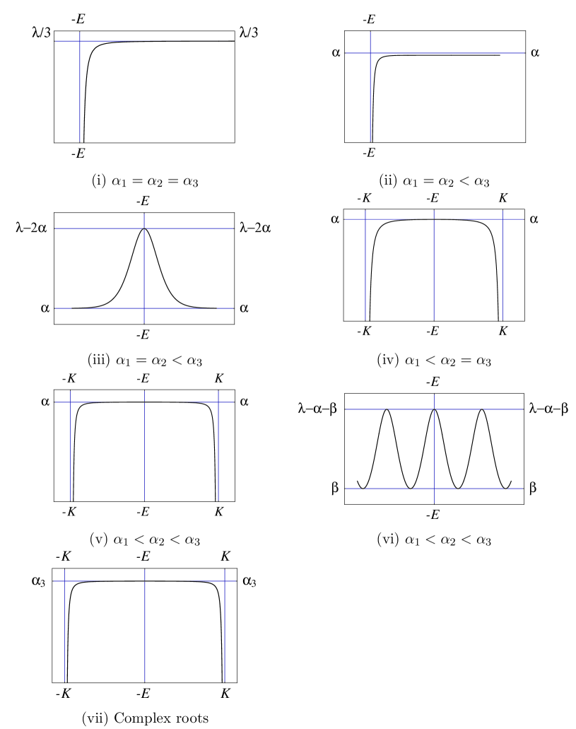
Figure 1: Curvature function for the different possibilities of the roots of the polynomial $P$. It is quite interesting to remark that in cases (i), (ii) and (iii), as $s$ increases, $k(s)$ approaches to a constant, said otherwise, the trajectory looks like a helix.

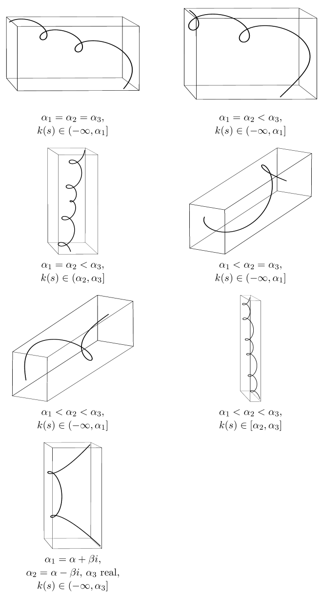
Figure 2: Worldlines for different curvature functions

References

- [1] M. S. Plyushchay. The model of the relativistic particle with torsion. Nuclear Phys. B, 362(1-2):54–72, 1991.
- [2] Yu. A. Kuznetsov and M. S. Plyushchay. The model of the relativistic particle with curvature and torsion. Nuclear Phys. B, 389(1):181–205, 1993.
- [3] M. S. Plyushchay. Massless particle with rigidity as a model for the description of bosons and fermions. Phys. Lett. B, 243(4):383–388, 1990.
- [4] M. S. Plyushchay. Does the quantization of a particle with curvature lead to the Dirac equation? Phys. Lett. B, 253(1-2):50–55, 1991.
- [5] A. A. Kapustnikov, A. Pashnev, and A. Pichugin. Canonical quantization of the kink model beyond the static solution. Phys. Rev. D, 55:2257–2264, 1997. hep-th/9608124
- [6] M. Barros. Geometry and dynamics of relativistic particles with rigidity. General Rel. Grav., 34:1–16, 2002.
- [7] A. Nersessian and E. Ramos. Massive spinning particles and the geometry of null curves. Phys. Lett. B, 445(1-2):123–128, 1998. hep-th/9807143
- [8] A. Nersessian and E. Ramos. A geometrical particle model for anyons. Modern Phys. Lett. A, 14(29):2033–2037, 1999. hep-th/9812077
- [9] S. Klishevich and M.S. Plyshchay. Zitterbewegung and reduction: 4d spinning particles and 3d anyons on light-like curves. Phys. Lett. B, 459:201–207, 1999. hep-th/9903102
- [10] A. Nerssesian, R. Manvelyan, and H.J.W. Müller-Kirsten. Particle with torsion on 3 null curves. Nucl. Phys. Proc. Suppl., 88:381–384, 2000. hep-th/9912061
- [11] A. Ferrández, A. Giménez, and P. Lucas. Null helices in Lorentzian space forms. International Journal of Modern Physics A, 16:4845–4863, 2001.
- [12] W. B. Bonnor. Null curves in a Minkowski spacetime. Tensor, N. S., 20:229–242, 1969.