CERN-TH/2002-116

Orbiting Strings in AdS Black Holes

and ${\cal N}=4$ SYM at Finite Temperature

A. Armoni,  J. L. F. Barbón  and  A. C. Petkou

Theory Division, CERN

CH-1211 Geneva 23, Switzerland

adi.armoni@cern.ch, barbon@cern.ch, tassos.petkou@cern.ch

Following Gubser, Klebanov and Polyakov [hep-th/0204051], we study strings in AdS black hole backgrounds. With respect to the pure AdS case, rotating strings are replaced by orbiting strings. We interpret these orbiting strings as CFT states of large spin similar to glueballs propagating through a gluon plasma. The energy and the spin of the orbiting string configurations are associated with the energy and the spin of states in the dual finite temperature ${\cal N}=4$ SYM theory. We analyse in particular the limiting cases of short and long strings. Moreover, we perform a thermodynamic study of the angular momentum transfer from the glueball to the plasma by considering string orbits around rotating AdS black holes. We find that standard expectations, such as the complete thermal dissociation of the glueball, are borne out after subtle properties of rotating AdS black holes are taken into account.

1 Introduction

The AdS/CFT conjecture [1, 2, 3] is used to make predictions about the strong coupling regime of ${\cal N}=4$ super Yang–Mills theory. However, most of the analysis done so far is restricted to the supergravity limit where the curvature is small and $\alpha^{\prime}{\cal R}$ corrections can be neglected (see [4] for a review).

Various ideas regarding extensions of the AdS/CFT correspondence beyond the supergravity limit have been put forward by Polyakov [5]. In another interesting recent development, the authors of [6] considered a particular limit of large $R$ charge where the sigma model is exactly solvable. Shortly afterwards GKP [7] have shown that the results of [6] can be rederived by considering appropriate configurations of classical rotating strings in ${\bf S}^{5}$, i.e. solitons of the nonlinear sigma model on $AdS_{5}\times{\bf S}^{5}$. Moreover, a rotation in the ${\bf S}^{3}$ inside the AdS₅ part of the metric was used to make a prediction about the anomalous dimensions of states as a function of their spin in the strong coupling limit, even at large spin !

The prescription is as follows: by using the Nambu–Goto action, the energy $E$ and the spin $S$ of a rotating string inside AdS₅ can be computed. The energy and spin are then re-interpreted as the energy and spin of twist two states in the boundary theory of the form

$$\Phi\nabla^{S}\Phi|\,0\,\rangle\;.$$ (1)

Such an interpretation is natural, since twist two states are dual to massive string modes, i.e. they are absent in the supergravity spectrum [8]. Then, due to conformal invariance the energy on ${\bf S}^{3}$ can be identified with the anomalous dimension $\Delta$ on ${\bf R}^{4}$. The remarkable result of GKP [7],

$$\Delta-S\approx\frac{\sqrt{\lambda}}{\pi}\ln\frac{S}{\sqrt{\lambda}}\,,$$ (2)

can be compared with the perturbative result for conformal gauge field theories [9, 10, 11]

$$\Delta-S=f(\lambda)\ln S\,,$$ (3)

where $f(\lambda)$ is a power series in $\lambda$. The analysis of GKP was afterwards extended beyond the Nambu–Goto action by [12] (see also [13]), confirming the $\ln S$ behavior beyond the $\lambda\rightarrow\infty$ limit.

This prescription is expected to hold for more general cases such as non-supersymmetric and non-conformal theories. Here we would like to calculate, using the GKP prescription, the relation between the energy and spin of states dual to string modes at finite temperature in ${\cal N}=4$ SYM. To this end we will consider the motion of classical strings in AdS₅ black hole background. In this case we cannot identify the energy with the scaling dimension, since we are considering a four-dimensional field theory on ${\bf S}^{3}\times{\bf S}^{1}$. The novel phenomenon is that physical states should be described by orbiting strings outside the black hole. We find corrections to the energy as a function of the spin both for short and long strings. Our main result is that states with large spin at large temperature, but $(RT)^{4}\sqrt{\lambda}\ll S$, obey the following relation

$$ER-S\approx{\sqrt{\lambda}\over 2\pi}\ln{S\over(RT)^{4}\sqrt{\lambda}}\,.$$ (4)

We also study the thermodynamical stability of these strings with respect to angular momentum leakage to the black hole. We find that these strings are unstable and eventually decay into a rotating black hole that harbours most of the initial spin. This leads to a natural interpretation of the decay process as the “melting” of a heavy glueball in the gluon plasma.

The organization of the manuscript is as follows: in section 2 we review the general prescription of GKP. Section 3 is devoted to the case of AdS₅ black hole. In section 4 we present our results for the specific limits of short and long strings. Finally, in section 5 we propose the gauge-theory interpretation of these results and study briefly the case of rotating AdS₅ black holes. In section 6 we present our conclusions.

2 Semiclassical orbiting strings in curved backgrounds

We consider semiclassical string motion in spherically symmetric 5-dimensional spacetimes whose general metric is of the form [14, 15]

$${\rm d}s^{2}=-f(r){\rm d}t^{2}+\frac{{\rm d}r^{2}}{f(r)}+r^{2}{\rm d}\Omega_{3}^{2}$$ (5)

$${\rm d}\Omega_{3}^{2}={\rm d}\theta^{2}+\sin^{2}\theta{\rm d}\phi_{1}^{2}+\cos^{2}\theta{\rm d}\phi_{2}^{2}$$ (6)

We are interested in the special cases

$$f(r)=1+\frac{r^{2}}{R^{2}} \rightarrow \mbox{AdS${}_{5}$ in global coordinates}\,,$$ (7)

$$f(r)=1+\frac{r^{2}}{R^{2}}-\frac{M}{r^{2}} \rightarrow \mbox{AdS${}_{5}$ black hole}\,.$$ (8)

The parameter $M$ is related to the black hole mass and for large temperatures we have $M/R^{2}\sim(RT)^{4}$ [16]. Consider classical string configurations extending in the radial $r$ direction of spacetime and rotating along the $\phi$ angle with constant angular velocity $\dot{\phi_{1}}=\dot{\phi}=\omega$, that is we consider circular orbits. This is achieved by choosing

$$X^{\mu}(\tau,\sigma)=(t,r(\sigma),\phi(t),{\pi\over 2},0)\,,$$ (9)

and by identifying $\tau$ and $t$. Then, the Nambu–Goto action

$$I=-{1\over 2\pi\alpha^{\prime}}\int{\rm d}\tau{\rm d}\sigma\sqrt{-\det G_{\mu\nu}\partial_{\alpha}X^{\mu}\partial_{\beta}X^{\nu}}\,,$$ (10)

takes the following form

$$I=-{1\over 2\pi\alpha^{\prime}}\int{\rm d}\tau\int{\rm d}\sigma\sqrt{-G_{rr}\left({dr\over d\sigma}\right)^{2}(G_{tt}+G_{\phi\phi}\dot{\phi}^{2})}\,.$$ (11)

which yields

$$I=-{1\over 2\pi\alpha^{\prime}}\int{\rm d}\tau\int_{r_{min}}^{r_{max}}{\rm d}r\sqrt{1-\dot{\phi}^{2}\frac{r^{2}}{f(r)}}\,.$$ (12)

The integration range $r_{min}\leq r\leq r_{max}$ is determined by the condition that the square root in (12) is real. For the spacetimes (7) and (8), this will be determined in terms of the parameters $\omega$ and $M$.

The energy and angular momentum of the string are then given by

$$E = {2\over 2\pi\alpha^{\prime}}\int_{r_{min}}^{r_{max}}{\rm d}r\frac{1}{\sqrt{1-\omega^{2}\frac{r^{2}}{f(r)}}}\,,$$ (13)

$$S = {2\over 2\pi\alpha^{\prime}}\int_{r_{min}}^{r_{max}}{\rm d}r\frac{\omega\frac{r^{2}}{f(r)}}{\sqrt{1-\omega^{2}\frac{r^{2}}{f(r)}}}\,.$$ (14)

The factor of two arises because the string is folded. Note that the setup in the presence of a horizon, see figure 1, is different from the AdS₅ case. In the latter, the string is folded around the origin and therefore a factor 4 arises in the expressions for energy and spin.

Throughout all intermediate calculations we will set the AdS radius $R=1$. The radius $R$ will be re-introduced in the final expressions.

3 The AdS₅ black hole background

We will be interested in strings in the AdS₅ black hole background. In the presence of the black hole horizon, the strings will rotate outside the horizon and not around the point $r=0$ as in the AdS case i.e. the strings are orbiting around the black hole.

Plugging the AdS₅ black hole metric (8) in (13) and (14) we obtain the following expressions

$$E = {1\over\pi\alpha^{\prime}}\int_{r_{min}}^{r_{max}}{\rm d}r\sqrt{r^{4}+r^{2}-M\over(1-\omega^{2})r^{4}+r^{2}-M}\,,$$ (15)

$$S = {1\over\pi\alpha^{\prime}}\int_{r_{min}}^{r_{max}}{\rm d}r{\omega r^{4}\over\sqrt{((1-\omega^{2})r^{4}+r^{2}-M)(r^{4}+r^{2}-M)}}\,.$$ (16)

Given $\omega^{2}$ one should guarantee that the expressions (15) and (16) are real. This requirement will set the boundaries of the integrals $r_{min}$ and $r_{max}$. Indeed by finding the roots of the quadratic equation

$$(1-\omega^{2})r^{4}+r^{2}-M=0\,,$$ (17)

one obtains

$$r_{\pm}^{2}=\frac{1}{2(\omega^{2}-1)}\left[1\pm\sqrt{1-4M(\omega^{2}-1)}\right]\,,$$ (18)

such that $r_{min}=r_{-}$ and $r_{max}=r_{+}$. In order to have real roots, we must constraint the possible values of $\omega^{2}$ as

$$\omega^{2}-1\leq{1\over 4M}\,.$$ (19)

A different way to find the physical condition (17) is to write the conformal constraints $T_{++}=T_{--}=0$ which give

$$G_{tt}+G_{\phi\phi}\omega^{2}+G_{rr}\left({dr\over d\sigma}\right)^{2}=0\,,$$ (20)

yielding

$$\left({dr\over d\sigma}\right)^{2}={(r^{4}(1-\omega^{2})+r^{2}-M)(r^{4}+r^{2}-M)\over r^{4}}\,.$$ (21)

The positivity of the rhs of (21) yields the physical constraints on the location of the string. In particular, at $r_{min},r_{max}$ the derivative with respect to $\sigma$ vanishes which gives (17).

In addition it is useful to write the roots of the equation

$$r^{4}+r^{2}-M=0\,,$$ (22)

as

$$r_{H}^{2}={1\over 2}(\sqrt{1+4M}-1)\,,\,\,\,\,-a^{2}=-{1\over 2}(\sqrt{1+4M}+1)\,,$$ (23)

where $r_{H}$ is the horizon. Note that $r_{-}>r_{H}$, such that the string orbits outside the black hole. The expressions for the energy and the spin can be written in the following form

$$E = {1\over\pi\alpha^{\prime}}\int_{r_{-}}^{r_{+}}{\rm d}r\sqrt{(r^{2}-r_{H}^{2})(r^{2}+a^{2})\over(\omega^{2}-1)(r^{2}-r_{-}^{2})(r_{+}^{2}-r^{2})}\,,$$ (24)

$$S = {1\over\pi\alpha^{\prime}}\int_{r_{-}}^{r_{+}}{\rm d}r{\omega r^{4}\over\sqrt{(\omega^{2}-1)(r^{2}-r_{-}^{2})(r_{+}^{2}-r^{2})(r^{2}-r_{H}^{2})(r^{2}+a^{2})}}\,.$$ (25)

The physical situation is described in figure 1 below.

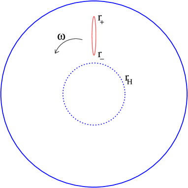
Figure 1: Spinning string in AdS₅ black hole background. The string stretches outside the black hole.

We give the explicit expressions for the integrals in the Appendix. In the next section we will discuss some specific cases.

4 Explicit solutions

4.1 Short strings

When $\omega^{2}\rightarrow\omega_{c}^{2}=1+{1\over 4M}$ (the critical value) the string shrinks to a point. In contrast to the pure AdS₅, in the AdS₅ black-hole case this solution corresponds to a particle which rotates outside the horizon. The location of the orbit is at $r_{+}^{2}=r_{-}^{2}=2M$.

The expressions for the energy and spin in this limit are given by

$$E={1\over\pi\alpha^{\prime}}\sqrt{4M^{2}+M\over 2}\int_{r_{-}}^{r_{+}}{dr\over\sqrt{(r_{+}-r)(r-r_{-})}}={1\over\alpha^{\prime}}\sqrt{4M^{2}+M\over 2}\,,$$ (26)

$$S={1\over\pi\alpha^{\prime}}\sqrt{2M^{2}}\int_{r_{-}}^{r_{+}}{dr\over\sqrt{(r_{+}-r)(r-r_{-})}}={1\over\alpha^{\prime}}\sqrt{2M^{2}}\,.$$ (27)

The relation between the energy and the spin, expressed in terms of the spin, becomes temperature independent

$$ER=S\sqrt{1+{\sqrt{\lambda}\over 2\sqrt{2}S}}\,.$$ (28)

For low temperatures, the large AdS₅ black-hole solution does not dominate over the thermal ensemble [16] and therefore the above expression is not valid for small $S$ (note that from (27) $S\sim T^{4}$). However, for large $S$ there should be states in the spectrum with the above relation between energy and spin. Namely, given a temperature $T$, there should exist a state with spin $S\sim T^{4}$ and energy $E$ such that their difference is a constant

$$ER-S\approx\sqrt{\lambda}\,.$$ (29)

4.2 Long strings

We would like to discuss now the interesting case of long strings. Long strings are achieved by taking $\omega^{2}\rightarrow 1$. We will parametrise the limit as

$$\omega^{2}=1+\eta,\,\,\,\,\eta\rightarrow 0\,.$$ (30)

In addition, we wish to take the high temperature limit

$${1\over 4M}=\epsilon,\,\,\,\,\epsilon\rightarrow 0\,,$$ (31)

and since $\omega^{2}\leq 1+{1\over 4M}$, we also choose

$${\eta\over\epsilon}\ll 1\,,$$ (32)

such that both the spin and the temperature are large, but the ratio of the temperature over the spin is small. The relevant parameters $r_{+},r_{-},a,r_{H}$ take the following values in this limit

$$r_{+}^{2}={1\over\eta},\,\,\,r_{-}^{2}={1\over 4\epsilon},\,\,\,a^{2}={1\over 2\sqrt{\epsilon}}+{1\over 2},\,\,\,r_{H}^{2}={1\over 2\sqrt{\epsilon}}-{1\over 2}\,.$$ (33)

The explicit expression for the energy is

$$E={1\over 2\pi\alpha^{\prime}}\int_{\sqrt{1\over 4\epsilon}}^{\sqrt{1\over\eta}}\sqrt{r^{4}+r^{2}\over\eta(r^{2}-{1\over 4\epsilon})({1\over\eta}-r^{2})}={1\over 2\pi\alpha^{\prime}}{1\over\eta}-{1\over 4\pi\alpha^{\prime}}\ln{\eta\over 4\epsilon}\,,$$ (34)

and for the spin

$$S={1\over 2\pi\alpha^{\prime}}\int_{\sqrt{1\over 4\epsilon}}^{\sqrt{1\over\eta}}{\omega r^{4}\over\sqrt{\eta(r^{2}-{1\over 4\epsilon})({1\over\eta}-r^{2})(r^{4}+r^{2})}}={1\over 2\pi\alpha^{\prime}}{1\over\eta}+{1\over 4\pi\alpha^{\prime}}\ln{\eta\over 4\epsilon}\,.$$ (35)

The equations (34), (35) lead to the following relation between the energy and the spin

$$ER-S\approx{\sqrt{\lambda}\over 2\pi}\ln{S\over(RT)^{4}\sqrt{\lambda}}\,.$$ (36)

This is our prediction for the energy of states with large spin at large temperature in the strong coupling limit. It is interesting to compare the above result (36) to the finite temperature correction to the Wilson loop [17, 18]. In both cases the correction to the solitonic state (open strings attached to the boundary in the Wilson loop case, or closed orbiting strings in the present case) involves a fourth power of the temperature.

Note also the similarity of (36) to the GKP result (2) for long strings at zero temperature and the difference by a factor of half in front of the logarithmic correction. This factor arises naturally since the present ’planetoid’ can be viewed as half of the GKP string after breaking into two pieces at the center of the $AdS$ due to the formation of a black hole. Notice however that for fixed spin the energy is minimized by a single planetoid.

5 CFT interpretation

The large AdS₅ black hole has a standard holographic interpretation as the canonical thermal ensemble of the CFT₄ on ${\bf S}^{3}$ at temperatures well above the critical temperature $T\gg 1/R$ [16]. At these temperatures the thermodynamic functions are well approximated by a “gluon plasma” of $O(N^{2})$ particle degrees of freedom. For example, the free energy scales as $F(T)/T\sim-N^{2}\,(R\,T)^{3}$. On the other hand, the sigma-model solitons representing the rotating strings have no significant degeneracy. They are associated to a single gauge-invariant state $|E,S\,\rangle$ in the Hilbert space of the CFT on ${\bf S}^{3}$ of energy $E$ and spin $S$. For $S\gg(R\,T)^{4}\sqrt{\lambda}$ we have a very long string with $E\approx S$ up to logarithmic corrections, just as in the zero-temperature theory. Hence, in the regime $S\gg(R\,T)^{4}\sqrt{\lambda}\gg 1$ we interpret the “planetoid string” orbiting the black hole as a large-$N$ approximation to the CFT state

$$\rho(T,E,S)=\rho_{T}\;\otimes\;\big{(}\,|E,S\rangle\,\langle E,S|\,\big{)}\;,$$ (37)

where

$$\rho_{T}={1\over Z(T)}\;e^{-H/T},\qquad Z(T)\equiv{\rm Tr}\,(\,\rho_{T}\,)\,,$$ (38)

is the density matrix of the canonical ensemble at temperature $T$. The direct product representation (37) is less and less accurate as $S$ approaches $(RT)^{4}\sqrt{\lambda}$. In fact, when $S\sim(RT)^{4}\sqrt{\lambda}$ the string degenerates to a point orbiting just above the horizon, and for smaller values of the spin there are no stable circular orbits that would represent stationary states. According to the UV/IR connection, this means that the typical length scales of the thermal ensemble and the gauge-invariant “glueball” state are well separated only for $S\gg(RT)^{4}\sqrt{\lambda}$. In this regime we have a very heavy glueball propagating in a thermal background. Since the glueball energy is much larger than the thermal energy density, the glueball propagates without much distortion, to leading order in the large-$N$ expansion. On the other hand, for $S\sim(RT)^{4}\sqrt{\lambda}$ we have $E\sim M$ and the glueball is considerably distorted by the thermal bath (it has degenerated to a pointlike object in AdS). Finally, for lower spins the glueball “melts” in the thermal bath and the corresponding string enters a spiral orbit and falls behind the black hole horizon.

This is a rather natural physical picture of the fate of heavy particles interacting with a background plasma. In fact, the apparent stability of the circular string orbit around the black hole should be an artifact of the large-$N$ limit. Effects of relative order $O(1/N^{2})$ should render the glueball unstable. This corresponds to interactions mediated by Feynman diagrams of toroidal topology in the CFT, or one-loop effects on the gravity side. At this order we have to consider for example the thermal Hawking radiation in equilibrium with the black hole. It is clear that both “gravitational bremsstrahlung” and the friction with the radiation will eventually damp the orbit of the “planetoid” and transfer angular momentum to the radiation. Microscopically, this process involves radiating small closed strings that fragment out of the lower endpoint of the long string (the local temperature is higher at the lower endpoint). For entropic reasons, a significant fraction of this dissipated angular momentum will end up in the black hole when the system relaxes to a stationary state. The precise mechanism of the decay will be complicated by the possibility of the long string fragmenting into large pieces first, with subsequent fragmentation into smaller ones or slow emission of short closed strings.

Thus, we conclude that the orbital strings considered in this paper are weakly unstable (within the $1/N$ expansion) towards falling into the black hole with the corresponding transfer of rotational energy. On the CFT side this process corresponds to the gradual melting of a heavy glueball by interactions with the thermal plasma. Eventually the glueball cannot be distinguished from thermal fluctuations and all the initial angular momentum is transferred to the plasma. The final stationary state is dual to a rotating AdS black hole such as those studied in [19].

In the next subsection we test this scenario by considering the orbits of stretched strings around rotating AdS black holes.

5.1 Strings in rotating AdS₅ black hole backgrounds and thermodynamical stability

Let us consider a thermal ensemble on ${\bf S}^{3}$ with grand canonical free energy $G(T,\Omega)$, where $\Omega$ is the chemical potential associated to the spin conserved quantum number $S$. It represents the average angular velocity of the thermal plasma around some axis in ${\bf S}^{3}$. If we work with the canonical free energy $F(T,S)$, evaluated as a function of the total spin we have

$$\Omega={\partial\,F(T,S)\over\partial\,S}\,\,.$$ (39)

Subluminal rotation of the thermal ensemble requires $\Omega<1$ (in units where $R=1$). In the dual AdS description, $\Omega$ is the angular velocity of a rotating AdS black hole (in a suitable reference frame).

Equilibrium with respect to angular momentum transfer between the rotating black hole and the rotating string is achieved when both chemical potentials are equal. The string “chemical potential” is nothing but its angular velocity

$$\omega={\partial\,E(S)\over\partial\,S}\,.$$ (40)

For long strings and slowly rotating black holes, we may approximate $E(S)$ by (36) and we obtain

$$\omega\approx 1+{\sqrt{\lambda}\over 2\pi S}\,.$$ (41)

This leads to the somewhat counterintuitive result that the long strings correspond to glueballs that rotate “faster than light” around ${\bf S}^{3}$. At any rate, the fact that $\omega>1>\Omega$ at very large $S$ means that the orbiting string is always unstable to spin transfer towards the static black hole. The stability condition

$$\omega=\Omega\,,$$ (42)

would require that eventually we reach a state where either $\Omega>1$ or $\omega<1$. The first option is actually excluded for stable black holes.

The purpose of this subsection is to investigate this question by studying equatorial circular orbits of strings around rotating AdS black holes. We consider a single common rotation axis and “parallel” rotations of both the string and the black hole. These constraints are natural for a process where the black hole angular momentum is entirely due to the transfer from the planetoid.

We consider rotating strings in the background of a Kerr AdS₅ black hole with a single rotation parameter $a_{1}=a$. The metric is given e.g. in Eq. 2.1 of [20]. Since the rotation of the string takes place along one of the circles of the AdS₅ black hole background, we only need to consider the above Kerr metric at $\theta=\pi/2$ and $\phi_{1}=\phi,\,\phi_{2}=0$. The resulting metric can then be put in the form

$${\rm d}s^{2} = -\frac{1}{r^{2}}(\Delta-a^{2}){\rm d}t^{2}+\frac{r^{2}}{\Delta}{\rm d}r^{2}+\frac{1}{r^{2}(1-a^{2})^{2}}[(r^{2}+a^{2})^{2}-a^{2}\Delta]{\rm d}\phi^{2}$$ (43)

$$+\frac{2a}{r^{2}(1-a^{2})}[\Delta-(r^{2}+a^{2})]{\rm d}t{\rm d}\phi\,,$$

$$\Delta = (r^{2}+a^{2})(1+r^{2})-M\,,$$ (44)

where again we set the AdS radius $R=1$.

There is a subtlety in the holographic map between this metric and the boundary CFT. In the given coordinates, the asymptotic sphere at infinity in (43) rotates with angular velocity $\Omega_{\infty}=-a$. In order to map the horizon angular velocity to the chemical potential $\Omega$ in the dual CFT it is convenient to subtract this inertial dragging of the boundary by redefining the angular coordinate

$$\varphi=\phi+a\,t\,.$$ (45)

In these new coordinates the asymptotic boundary of the Kerr AdS spacetime is static and the angular velocity of the black hole is

$$\Omega=\Omega_{H}-\Omega_{\infty}=\frac{a(1+{r}_{H}^{2})}{{r}_{H}^{2}+a^{2}}\,,$$ (46)

with the horizon radius ${r}_{H}$ given by the largest solution of the equation

$$({r}_{H}^{2}+a^{2})(1+{r}_{H}^{2})=M\,.$$ (47)

In [20] it was shown that the black hole free energy diverges as $\Omega\rightarrow 1$ from below

$$F/T\sim-{N^{2}\over 1-\Omega^{2}}\,(R\,T)^{3}\;.$$ (48)

Hence, the strongly-coupled CFT can only tolerate chemical potentials in the range $\Omega^{2}<1$: it takes infinite free energy to raise the angular velocity to the speed of light on the boundary ${\bf S}^{3}$.

It is interesting to note that one can have $|\Omega|>1$ for black holes with negative specific heat. The situation regarding the angular velocity in the boundary theory is analogous to the occurrence of $\omega>1$ for rotating strings that eventually become unstable.

The metric (43) is of the general axisymmetric form

$${\rm d}s^{2}=G_{tt}{\rm d}t^{2}+G_{rr}{\rm d}r^{2}+G_{\phi\phi}{\rm d}\phi^{2}+2\,G_{t\phi}{\rm d}t{\rm d}\phi\,.$$ (49)

Using the gauge (9) we can also easily derive integral formulas for the energy, angular momentum and action of strings in (49) as

$$E = \frac{1}{\pi\alpha^{\prime}}\int_{r_{min}}^{r_{\max}}{\rm d}r\frac{-G_{rr}\left(G_{tt}+\omega G_{t\phi}\right)}{\sqrt{V}}\,,$$ (50)

$$S = \frac{1}{\pi\alpha^{\prime}}\int_{r_{min}}^{r_{\max}}{\rm d}r\frac{G_{rr}\left(\omega G_{\phi\phi}+G_{t\phi}\right)}{\sqrt{V}}\,,$$ (51)

$$I = -{2\over\omega\alpha^{\prime}}\int_{r_{min}}^{r_{max}}{\rm d}r\sqrt{V}\;.$$ (52)

The effective potential $V$ is given by

$$V\equiv-G_{rr}\,\left(G_{tt}+2\omega G_{t\phi}+\omega^{2}\,G_{\phi\phi}\right)\,.$$ (53)

From the integral representations one can prove the relations

$$-{\omega\,I\over 2\pi}=E-\omega\,S,\qquad S=-{\partial\over\partial\omega}\,\left(-{\omega\,I\over 2\pi}\right)\,.$$ (54)

This means that $-\omega I(\omega)/2\pi$ is the Legendre transform $E(S)$ of the energy as a function of the spin. Hence, one has the desired relation between the angular velocity of the string and the “spin dispersion relation”

$$\omega={\partial E(S)\over\partial S}\;.$$ (55)

Explicitly, for the Kerr metric (43) we find the effective potential

$$V=\frac{1-(\omega+a)^{2}}{\Delta(1-a^{2})}\left[r^{4}+\left(\frac{1-a^{2}(\omega+a)^{2}}{1-(\omega+a)^{2}}\right)r^{2}-\left(\frac{(1-a(\omega+a))^{2}}{1-(\omega+a)^{2}}\right)\frac{M}{1-a^{2}}\right]\;.$$ (56)

From (56) we see that it is natural to redefine the angular velocity for the string as

$$\omega+a\longrightarrow\omega\,.$$ (57)

This is the angular velocity of the string in the coordinate system corresponding to the change of variables $\phi=\varphi-a\,t$, exactly the same as in (45). Hence, it is the shifted angular velocity as in (57), defined by $\varphi(t)=\omega\,t$, the one that must be compared directly to the thermal chemical potential $\Omega$.

Given the fact that $\Omega<1$ for the stable black holes that we are considering, the stability question reduces to whether a non-vanishing rotation parameter of the black hole $a>0$ can induce finite-energy string orbits with $\omega<1$.

In order to answer this question, we calculate the turning points $r_{min}=r_{-}$ and $r_{max}=r_{+}$ from the equation $V=0$. The result is

$$r_{\pm}^{2}={1-a^{2}\omega^{2}\over 2(\omega^{2}-1)}\;\left[\;1\pm\sqrt{1-{4M(\omega^{2}-1)\over(1-a^{2})\,(1+a\omega)^{2}}}\;\right]\;.$$ (58)

This expression shows that at soon as $\omega^{2}<1$ the outer endpoint $r_{+}$ becomes imaginary for any value of $a^{2}\leq 1$. This means that we must necessarily have $\omega^{2}>1$ and no stability is possible between the planetoid and the rotating black hole.

It is interesting to obtain the rough features of the orbits. For $\omega>1$ the condition that $r_{\pm}^{2}>0$ and real is that $\omega<1/a$ and that the argument of the square root in (58) be positive. The second condition defines a maximal angular velocity $\omega_{c}$ that can be explicitly calculated as a function of $a$ and $M$. For large black hole masses (large temperature) one obtains

$$\omega_{c}=1+(1-a)\,\left[{(1+a)^{3}\over 8M}+\dots\right]\;.$$ (59)

The overall factor of $(1-a)$ arises from the fact that $a=1$ requires $\omega_{c}=1$.

From the expression (59) we can deduce that the condition $\omega<1/a$ is redundant. This condition can only be relevant for $a$ close to unity. Let $a=1-\epsilon$, $1/a\approx 1+\epsilon$. Then for large mass one has

$$\omega_{c}\approx 1+{\epsilon\over M}<1+\epsilon\approx 1/a\,,$$ (60)

and we see that the relevant interval of angular velocities is $1<\omega<\omega_{c}$.

The rough features of the planetoids are similar to those at $a=0$. As $\omega\rightarrow\omega_{c}$ from below the string degenerates to a point orbiting at

$$r^{2}_{+}=r^{2}_{-}=2M{(1-a\omega_{c})^{2}\over(1-a^{2})^{2}}\;.$$ (61)

For large $M$, this becomes by virtue of (59)

$$r^{2}_{+}=r^{2}_{-}\rightarrow{2M\over(1+a)^{2}}\;.$$ (62)

On the other hand, for $\omega\rightarrow 1$ from above the upper endpoint tends to infinity $r_{+}\rightarrow\infty$ and the lower endpoint descends to the minimum value

$$r^{2}_{-}\rightarrow{M\over(1+a)^{2}}\;.$$ (63)

For $M\gg 1$ the horizon sits at $r^{2}_{H}\sim\sqrt{M}$ and the planetoid is well above the black hole in any of these limits.

Our main result of this section is that $\Omega<1<\omega$ for finite-energy orbiting strings and stable black holes with positive specific heat. This means that no equilibrium configuration exists with respect to angular-momentum balance and the planetoid will eventually fall behind the rotating black hole horizon. It would be interesting to study the fate of string orbits around “small” AdS black holes with negative specific heat. In this case one can have $\Omega>1$ so that stable orbits are possible, although the black hole itself is unstable.

We have also assumed in our analysis that the orbits were “direct”, i.e. the black hole and the planetoid rotate in the same sense. One can also consider “retrograde” orbits satisfying $\omega\,\Omega<0$. In this case the final black-hole spin is not entirely due to the transfer from the planetoid.

6 Conclusions

We have studied finite temperature effects on the physics of certain large spin states of ${\cal N}=4$ SYM on a three sphere. In the formalism of GKP [7] these states correspond to folded closed strings rotating in AdS space. The finite temperature generalization amounts to the study of similar string configurations in the background of AdS black holes. The main novelty is that the black hole turns the rotating strings into orbiting strings or “planetoids” [14].

These planetoids stay clear from the black hole horizon and represent thermally perturbed gauge-invariant states of large energy satisfying $E\sim S$ with logarithmic accuracy. Since they correspond to closed-string states we term them “glueballs”. When the glueball mass is of the order of the thermal energy per gauge degree of freedom we expect that the glueball should melt or dissociate in the plasma. This physics is reflected in the gravitational dual by the degeneration of the stringy planetoid to a pointlike object rotating not far above the horizon. This configuration represents the circular orbit of lowest spin for a given temperature. All lower orbits decay into the black hole. Nevertheless, for “long string” configurations, the corresponding states have energy and spin much larger than the black hole mass and could represent quasi-stable glueball states propagating in the thermal bath. For such states our strong coupling prediction for their energy and spin is (4).

In subleading orders in the $1/N$ expansion, interaction with the Hawking thermal radiation should destabilise any orbit, leading to the progressive melting of the fast glueball into the plasma. We have checked this idea in the gravity dual by studying orbiting strings around rotating AdS black holes. We find that the transfer of angular momentum from the planetoid to the black hole is always thermodynamically favoured. Hence, the heavy glueball eventually melts and transfers all its angular momentum to the thermal bath.

It would be interesting to study in more detail the fate of the low temperature GKP soliton across the Hawking-Page phase transition. In particular the dynamics of string fragmentation versus black hole formation.

These systems provide a very interesting example of the AdS/CFT correspondence, where one can describe the interaction between very special states with peculiar properties and typical (featureless) states such as a thermal density matrix. Once again, a somewhat exotic gravitational dynamics on the AdS side encodes very nontrivial, yet physically reasonable effects on the CFT side.

ACKNOWLEDGEMENTS

We would like to thank E. Gardi and S. Wadia for illuminating discussions. We also thank A. Tseytlin for the critical reading of an earlier version of the manuscript.

Appendix

We start with the evaluation of (24). Setting $r^{2}=x$ we obtain

$$E=\frac{1}{2\pi\alpha^{\prime}\sqrt{\omega^{2}-1}}\int_{x_{-}}^{x_{+}}{\rm d}x\,\sqrt{\frac{(x-x_{H})(x+A)}{x(x-x_{-})(x_{+}-x)}}\,,x_{\pm}=r^{2}_{\pm}\,,x_{H}=r^{2}_{H}\,,A=a^{2}$$ (64)

Then we set $\rho=x-x_{-}$ to obtain

$$E=\frac{1}{2\pi\alpha^{\prime}\sqrt{\omega^{2}-1}}\int_{0}^{\rho_{+}}{\rm d}\rho\sqrt{\frac{(\rho+x_{-}-x_{H})(\rho+A+x_{-})}{\rho(\rho+x_{-})(\rho_{+}-\rho)}}\,,\,\,\,\,\rho_{+}=r_{+}^{2}-r_{-}^{2}$$ (65)

Finally, we set $t=\rho/\rho_{+}$ to get

$$E=\frac{\sqrt{\rho_{+}}}{2\pi\alpha^{\prime}\sqrt{\omega^{2}-1}}\int_{0}^{1}{\rm d}t\sqrt{\frac{\left(t+\frac{x_{-}-x_{H}}{\rho_{+}}\right)\left(t+\frac{A+x_{-}}{\rho_{+}}\right)}{t(1-t)\left(t+\frac{x_{-}}{\rho_{+}}\right)}}$$ (66)

Similar calculations lead to the following expression for the spin (25)

$$S=\frac{\omega\sqrt{\rho_{+}}}{2\pi\alpha^{\prime}\sqrt{\omega^{2}-1}}\int_{0}^{1}{\rm d}t\frac{\left(t+\frac{x_{-}}{\rho_{+}}\right)^{\frac{3}{2}}}{\sqrt{t(1-t)\left(t+\frac{x_{-}-x_{H}}{\rho_{+}}\right)\left(t+\frac{A+x_{-}}{\rho_{+}}\right)}}$$ (67)

Clearly, the above two expressions may be considered as representing generalized hypergeometric series in the three variables $x_{-}/\rho_{+}$, $(x_{-}-x_{H})/\rho_{+}$ and $(A+x_{-})/\rho_{+}$. Nevertheless, in the interesting cases of long and short strings the expressions simplify.

a) Short strings. In this case $\omega\rightarrow\omega_{c}$ and $\rho_{+}\rightarrow 0$ therefore the relevant representations of (65) and (67) are

$$E = \frac{1}{2\pi\alpha^{\prime}\sqrt{\omega^{2}-1}}\sqrt{\frac{(x_{-}-x_{H})(A+x_{-})}{x_{-}}}\int_{0}^{1}{\rm d}t\sqrt{\frac{\left(1+t\frac{\rho_{+}}{x_{-}-x_{H}}\right)\left(1+t\frac{\rho_{+}}{A+x_{-}}\right)}{t(1-t)\left(1+t\frac{\rho_{+}}{x_{-}}\right)}}$$ (68)

$$S = \frac{\omega}{2\pi\alpha^{\prime}\sqrt{\omega^{2}-1}}\frac{(x_{-})^{\frac{3}{2}}}{\sqrt{(x_{-}-x_{H})(A+x_{-})}}\int_{0}^{1}{\rm d}t\sqrt{\frac{\left(1+t\frac{\rho_{+}}{x_{-}}\right)^{3}}{t(1-t)\left(1+t\frac{\rho_{+}}{x_{-}-x_{H}}\right)\left(1+t\frac{\rho_{+}}{A+x_{-}}\right)}}$$

Then, given the fact that

$$\omega_{c}^{2}-1=\frac{1}{4M}$$ (70)

we find

$$(x_{-}-x_{H})(A+x_{-})=4M^{2}\left(1+\frac{1}{4M}\right)$$ (71)

and taking the $\rho_{+}\rightarrow 0$ limit of (68) and (LABEL:Spshort) we obtain

$$E = \sqrt{2\lambda}M\left(1+\frac{1}{4M}\right)^{1/2}$$ (72)

$$S = \sqrt{2\lambda}M$$ (73)

This leads to

$$ER=S\left(1+\frac{\sqrt{\lambda}}{2\sqrt{2}S}\right)^{1/2}$$ (74)

b) Long strings. In this case we set $\omega^{2}-1=\eta$ with $\eta\rightarrow 0$ and we obtain from the explicit expressions above

$$E = \frac{\sqrt{\rho_{+}}}{2\pi\alpha^{\prime}\sqrt{\eta}}\int_{0}^{1}{\rm d}t\sqrt{\frac{\left(t+\frac{x_{-}}{\rho_{+}}\right)}{t(1-t)}}\left[1+\frac{A-x_{H}}{\rho_{+}}\left(t+\frac{x_{-}}{\rho_{+}}\right)^{-1}-\frac{x_{H}A}{\rho_{+}^{2}}\left(t+\frac{x_{-}}{\rho_{+}}\right)^{-2}\right]^{\frac{1}{2}}$$

$$S = \frac{\omega\sqrt{\rho_{+}}}{2\pi\alpha^{\prime}\sqrt{\eta}}\int_{0}^{1}{\rm d}t\sqrt{\frac{\left(t+\frac{x_{-}}{\rho_{+}}\right)}{t(1-t)}}\left[1+\frac{A-x_{H}}{\rho_{+}}\left(t+\frac{x_{-}}{\rho_{+}}\right)^{-1}-\frac{x_{H}A}{\rho_{+}^{2}}\left(t+\frac{x_{-}}{\rho_{+}}\right)^{-2}\right]^{-\frac{1}{2}}$$

From the above we easily see that the leading divergence is the same for both $E$ and $S$ and equal to

$$E_{0}=S_{0}\approx\frac{\sqrt{\lambda}}{\eta}$$ (77)

To evaluate the corrections to the leading divergence we consider the difference $E-S$. From the above it is not difficult to see that the leading term in that difference is

$$E-S\approx{1\over 2\alpha^{\prime}}\left(1+M\eta\right)^{-\frac{1}{2}}{}_{2}F_{1}\left(\frac{1}{2},\frac{1}{2};1;\frac{1}{1+M\eta}\right)$$ (78)

In the limit $M\eta\rightarrow 0$ the hypergeometric function has a logarithmic behavior that leads to

$$ER-S\approx\frac{\sqrt{\lambda}}{2\pi}\ln\frac{S}{M\sqrt{\lambda}}\sim\frac{\sqrt{\lambda}}{2\pi}\ln\frac{S}{(RT)^{4}\sqrt{\lambda}}.$$ (79)

References

- [1] J. M. Maldacena, “The large limit of superconformal field theories and supergravity,” Adv. Theor. Math. Phys. 2, 231 (1998) [Int. J. Theor. Phys. 38, 1113 (1999)] [arXiv:hep-th/9711200].
- [2] S. S. Gubser, I. R. Klebanov and A. M. Polyakov, “Gauge theory correlators from non-critical string theory,” Phys. Lett. B 428, 105 (1998) [arXiv:hep-th/9802109].
- [3] E. Witten, “Anti-de Sitter space and holography,” Adv. Theor. Math. Phys. 2, 253 (1998) [arXiv:hep-th/9802150].
- [4] O. Aharony, S. S. Gubser, J. M. Maldacena, H. Ooguri and Y. Oz, “Large N field theories, string theory and gravity,” Phys. Rept. 323, 183 (2000) [arXiv:hep-th/9905111].
- [5] A. M. Polyakov, “Gauge fields and space-time,” arXiv:hep-th/0110196.
- [6] D. Berenstein, J. M. Maldacena and H. Nastase, “Strings in flat space and pp waves from N = 4 super Yang Mills,” JHEP 0204, 013 (2002) [arXiv:hep-th/0202021].
- [7] S. S. Gubser, I. R. Klebanov and A. M. Polyakov, “A semi-classical limit of the gauge/string correspondence,” arXiv:hep-th/0204051.
- [8] G. Arutyunov, S. Frolov and A. C. Petkou, “Operator product expansion of the lowest weight CPOs in N = 4 SYM(4) at strong coupling,” Nucl. Phys. B 586, 547 (2000) [Erratum-ibid. B 609, 539 (2001)] [arXiv:hep-th/0005182].
- [9] E. G. Floratos, D. A. Ross and C. T. Sachrajda, “Higher Order Effects In Asymptotically Free Gauge Theories: The Anomalous Dimensions Of Wilson Operators,” Nucl. Phys. B 129, 66 (1977) [Erratum-ibid. B 139, 545 (1978)].
- [10] G. P. Korchemsky, “Asymptotics Of The Altarelli-Parisi-Lipatov Evolution Kernels Of Parton Distributions,” Mod. Phys. Lett. A 4, 1257 (1989).
- [11] F. A. Dolan and H. Osborn, “Superconformal symmetry, correlation functions and the operator product expansion,” Nucl. Phys. B 629, 3 (2002) [arXiv:hep-th/0112251].
- [12] S. Frolov and A. A. Tseytlin, “Semiclassical quantization of rotating superstring in AdS(5) x S**5,” arXiv:hep-th/0204226.
- [13] J. G. Russo, “Anomalous dimensions in gauge theories from rotating strings in ,” arXiv:hep-th/0205244.
- [14] H. J. de Vega and I. L. Egusquiza, “Planetoid String Solutions in 3 + 1 Axisymmetric Spacetimes,” Phys. Rev. D 54, 7513 (1996) [arXiv:hep-th/9607056].
- [15] S. Kar and S. Mahapatra, “Planetoid strings: Solutions and perturbations,” Class. Quant. Grav. 15, 1421 (1998) [arXiv:hep-th/9701173].
- [16] E. Witten, “Anti-de Sitter space, thermal phase transition, and confinement in gauge theories,” Adv. Theor. Math. Phys. 2, 505 (1998) [arXiv:hep-th/9803131].
- [17] S. J. Rey, S. Theisen and J. T. Yee, “Wilson-Polyakov loop at finite temperature in large N gauge theory and anti-de Sitter supergravity,” Nucl. Phys. B 527, 171 (1998) [arXiv:hep-th/9803135].
- [18] A. Brandhuber, N. Itzhaki, J. Sonnenschein and S. Yankielowicz, “Wilson loops in the large N limit at finite temperature,” Phys. Lett. B 434, 36 (1998) [arXiv:hep-th/9803137].
- [19] S. W. Hawking, C. J. Hunter and M. M. Taylor-Robinson, “Rotation and the AdS/CFT correspondence,” Phys. Rev. D 59, 064005 (1999) [arXiv:hep-th/9811056].
- [20] S. W. Hawking and H. S. Reall, “Charged and rotating AdS black holes and their CFT duals,” Phys. Rev. D 61 (2000) 024014 [arXiv:hep-th/9908109].