Inflationary Theory versus Ekpyrotic/Cyclic Scenario

Abstract

I will discuss the development of inflationary theory and its present status, as well as some recent attempts to suggest an alternative to inflation. In particular, I will argue that the ekpyrotic scenario in its original form does not solve any of the major cosmological problems. Meanwhile, the cyclic scenario is not an alternative to inflation but rather a complicated version of inflationary theory. This scenario does not solve the flatness and entropy problems, and it suffers from the singularity problem. We describe many other problems that need to be resolved in order to realize a cyclic regime in this scenario, produce density perturbations of a desirable magnitude, and preserve them after the singularity. We propose several modifications of this scenario and conclude that the best way to improve it is to add a usual stage of inflation after the singularity and use that inflationary stage to generate perturbations in the standard way. This modification significantly simplifies the cyclic scenario, eliminates all of its numerous problems, and makes it equivalent to the usual chaotic inflation scenario.

]

Contents

toc

I Introduction

My first encounter with Stephen Hawking was related to inflationary theory. It was quite dramatic. In the middle of October 1981 there was a conference on Quantum Gravity in Moscow. This was the first conference where I gave a talk on the new inflation scenario [1]. After my talk many participants of the conference from the USA and Europe came up to me, asked questions, and even suggested smuggling my paper abroad to speed up its publication. (The paper was written in July 1981, but in accordance with Russian rules I spent 3 months getting permission for its publication.)

Somehow I did not have a chance to discuss it with Stephen at the conference, but we did it the next day, under rather unusual circumstances. He was invited to give a talk at the Sternberg Astronomy Institute of Moscow State University. His talk, based on his work with Moss and Stewart [2], was about the problems of the old inflationary theory proposed by Alan Guth [3]. The main conclusion of their work [2], as well as of the subsequent paper by Guth and Weinberg [4], was that it is impossible to improve the old inflation scenario.

Rather unexpectedly, I was asked to translate. At that time Stephen did not have his computer, so his talks usually were given by his students. He would just sit around and add brief comments if a student would say something wrong. This time, however, they were not quite prepared. Stephen would say one word, his student would say one word, and then I would translate this word, so in the beginning the talk progressed very slowly. Since I knew the subject, I started adding lengthy explanations in Russian. Thus, Stephen would say one word, his student would say one word, and then I would talk for few minutes. Then Stephen would talk again, etc. Everything went smoothly during the first part of the talk when we were explaining the problems of the old inflationary theory.

Then Stephen said that recently Andrei Linde had suggested an interesting way to solve the problems of inflationary theory. I happily translated this. The best physicists of Russia are here to listen to Stephen, my future depends on them, and now he is going to explain my work to them; what could be better? But then Stephen said that the new inflationary scenario cannot work… and I translated. For the next half hour I was translating for Stephen and explaining to everyone the problems with my scenario and why it does not work…

I do not remember ever being in any other situation like that. What shall I do, what shall I do?.. When the talk was over I said that I translated but I disagree, and explained why. Then I suggested to Stephen that we discuss it privately. We found an empty office and for almost two hours the authorities of the Institute were in a panic searching for the famous British scientist who had miraculously disappeared. Meanwhile I was talking to him about various parts of the new inflationary scenario. From time to time Stephen would say something and his student would translate: “But you did not say that before.” This was repeated over and over again. Then Stephen invited me to his hotel where we continued the discussion. Then he started showing me photos of his family and invited me to Cambridge. This was the beginning of a beautiful friendship.

After that event the story developed at a rapid pace. In October I sent my paper to Physics Letters and I also sent my preprints to many places in the USA. After returning to England Stephen started working on new inflation together with Ian Moss [5]. Three months later, Paul Steinhardt and Andy Albrecht wrote a paper on new inflation with results very similar to mine [6]. In Summer 1982 Stephen organized a workshop in Cambridge dedicated to new inflation. This was the best and most productive workshop I have ever attended.

In a certain sense, this was the first and the last workshop on new inflation. The theory of inflationary perturbations of scalar fields [7, 8], as well as the theory of post-inflationary density perturbations [9, 10, 11], were to a large extent developed at this workshop [10]. Calculations using these theories showed that the coupling constant of the scalar field in new inflation had to be smaller than $10^{-12}$. Such a field could not be in a state of thermal equilibrium in the early universe. This means, in particular, that the theory of high-temperature phase transitions [12], which served as the basis for old and new inflation, was in fact irrelevant for inflationary cosmology. Thus, some other approach was necessary. The assumption of thermal equilibrium requires many particles interacting with each other. This means that new inflation could explain why our universe was so large only if it was very large from the beginning. Finally, inflation in this theory begins very late, and during the preceding epoch the universe could easily have collapsed or become so inhomogeneous that inflation could never happen. In addition, this scenario could work only if the effective potential of the field $\phi$ had a very flat plateau near $\phi=0$, which is somewhat artificial. Because of all of these difficulties, no realistic versions of the new inflationary universe scenario have been proposed so far.

From a more general perspective, old and new inflation represented a substantial but incomplete modification of the big bang theory. It was still assumed that the universe was in a state of thermal equilibrium from the very beginning, that it was relatively homogeneous and large enough to survive until the beginning of inflation, and that the stage of inflation was just an intermediate stage of the evolution of the hot universe. In the beginning of the 80’s these assumptions seemed natural and practically unavoidable. That is why it was so difficult to overcome a certain psychological barrier and abandon all of these assumptions. This was done with the invention of the chaotic inflation scenario [13]. This scenario resolved all the problems mentioned above. According to this scenario, inflation can occur even in theories with the simplest potentials such as $V(\phi)\sim\phi^{n}$. Inflation can begin even if there was no thermal equilibrium in the early universe, and it can even start close to the Planck density, in which case the problem of initial conditions for inflation can be easily resolved [14].

Stephen was the first person (apart from my Russian colleagues) to whom I spoke about chaotic inflation. Since that time in his work on inflation he has used only this model, as well as some modifications of the Starobinsky scenario [15]. Let me describe the basic features of chaotic inflation.

II Chaotic inflation

Consider the simplest model of a scalar field $\phi$ with a mass $m$ and with the potential energy density $V(\phi)={m^{2}\over 2}\phi^{2}$. Since this function has a minimum at $\phi=0$, one may expect that the scalar field $\phi$ should oscillate near this minimum. This is indeed the case if the universe does not expand, in which case equation of motion for the scalar field coincides with equation for harmonic oscillator, $\ddot{\phi}=-m^{2}\phi$.

However, because of the expansion of the universe with Hubble constant $H=\dot{a}/a$, an additional term $3H\dot{\phi}$ appears in the harmonic oscillator equation:

$$\ddot{\phi}+3H\dot{\phi}=-m^{2}\phi\ .$$ (1)

The term $3H\dot{\phi}$ can be interpreted as a friction term. The Einstein equation for a homogeneous universe containing scalar field $\phi$ looks as follows:

$$H^{2}+{k\over a^{2}}={1\over 6}\,\left(\dot{\phi}^{2}+m^{2}\phi^{2})\right)\ .$$ (2)

Here $k=-1,0,1$ for an open, flat or closed universe respectively. We work in units $M_{p}^{-2}=8\pi G=1$.

If the scalar field $\phi$ initially was large, the Hubble parameter $H$ was large too, according to the second equation. This means that the friction term $3H\dot{\phi}$ was very large, and therefore the scalar field was moving very slowly, as a ball in a viscous liquid. Therefore at this stage the energy density of the scalar field, unlike the density of ordinary matter, remained almost constant, and expansion of the universe continued with a much greater speed than in the old cosmological theory. Due to the rapid growth of the scale of the universe and a slow motion of the field $\phi$, soon after the beginning of this regime one has $\ddot{\phi}\ll 3H\dot{\phi}$, $H^{2}\gg{k\over a^{2}}$, $\dot{\phi}^{2}\ll m^{2}\phi^{2}$, so the system of equations can be simplified:

$$H={\dot{a}\over a}={m\phi\over\sqrt{6}}\ ,~{}~{}~{}~{}~{}~{}\dot{\phi}=-m\ \sqrt{2\over 3}.$$ (3)

The first equation shows that if the field $\phi$ changes slowly, the size of the universe in this regime grows approximately as $e^{Ht}$, where $H={m\phi\over\sqrt{6}}$. This is the stage of inflation, which ends when the field $\phi$ becomes much smaller than $M_{p}=1$. Solution of these equations shows that after a long stage of inflation the universe initially filled with the field $\phi=\phi_{0}\gg 1$ grows exponentially [14],

$$a=a_{0}\ e^{\phi_{0}^{2}/4}.$$ (4)

This is as simple as it could be. Inflation does not require supercooling and tunneling from the false vacuum [3], or rolling from an artificially flat top of the effective potential [1, 6]. It appears in the theories that can be as simple as a theory of harmonic oscillator [13]. Only after I realized it, I started to believe that inflation is not a trick necessary to fix problems of the old big bang theory, but a generic cosmological regime.

In realistic versions of inflationary theory the duration of inflation could be as short as $10^{-35}$ seconds. When inflation ends, the scalar field $\phi$ begins to oscillate near the minimum of $V(\phi)$. As any rapidly oscillating classical field, it looses its energy by creating pairs of elementary particles. These particles interact with each other and come to a state of thermal equilibrium with some temperature $T$ [17, 18, 19]. From this time on, the universe can be described by the usual big bang theory.

The main difference between inflationary theory and the old cosmology becomes clear when one calculates the size of a typical inflationary domain at the end of inflation. Investigation of this question shows that even if the initial size of inflationary universe was as small as the Plank size $l_{P}\sim 10^{-33}$ cm, after $10^{-35}$ seconds of inflation the universe acquires a huge size of $l\sim 10^{10^{12}}$ cm! This number is model-dependent, but in all realistic models the size of the universe after inflation appears to be many orders of magnitude greater than the size of the part of the universe which we can see now, $l\sim 10^{28}$ cm. This immediately solves most of the problems of the old cosmological theory [13, 14].

Our universe is almost exactly homogeneous on large scale because all inhomogeneities were exponentially stretched during inflation. The density of primordial monopoles and other undesirable “defects” becomes exponentially diluted by inflation. The universe becomes enormously large. Even if it was a closed universe of a size $\sim 10^{-33}$ cm, after inflation the distance between its “South” and “North” poles becomes many orders of magnitude greater than $10^{28}$ cm. We see only a tiny part of the huge cosmic balloon. That is why nobody has ever seen how parallel lines cross. That is why the universe looks so flat.

If our universe initially consisted of many domains with chaotically distributed scalar field $\phi$ (or if one considers different universes with different values of the field), then domains in which the scalar field was too small never inflated. The main contribution to the total volume of the universe will be given by those domains which originally contained large scalar field $\phi$. Inflation of such domains creates huge homogeneous islands out of initial chaos. Each homogeneous domain in this scenario is much greater than the size of the observable part of the universe.

FIG. 1.: The harmonic oscillator scalar field potential $V(\phi)=V_{0}+m^{2}\phi^{2}/2$ in a simplest version of chaotic inflation.

Now let us make another simple step and add a small constant term $V_{0}>0$ to the potential $m^{2}\phi^{2}/2$, see Fig. 1. If one does not take gravity into account, this term does not change equations for the scalar field, i.e. we still consider a simplest harmonic oscillator theory. However, the term $V_{0}$ acts as a cosmological constant that does not vanish even at $\phi=0$. As a result, the simplest theory with $V(\phi)=V_{0}+m^{2}\phi^{2}/2$ will describe two stages of inflation. The first stage occurs in the early universe, when the scalar field was large. The second stage occurs right now; it corresponds to the recently discovered accelerated expansion of the universe, see Fig. 2.

The first models of chaotic inflation were based on the theories with polynomial potentials, such as $V(\phi)=\pm{m^{2}\over 2}\phi^{2}+{\lambda\over 4}\phi^{4}$. But the main idea of this scenario is quite generic. One should consider any particular potential $V(\phi)$, polynomial or not, with or without spontaneous symmetry breaking, and study all possible initial conditions without assuming that the universe was in a state of thermal equilibrium, and that the field $\phi$ was in the minimum of its effective potential from the very beginning [13]. This scenario strongly deviated from the standard lore of the hot big bang theory and was psychologically difficult to accept. Therefore during the first few years after invention of chaotic inflation many authors claimed that the idea of chaotic initial conditions is unnatural, and made attempts to realize the new inflation scenario based on the theory of high-temperature phase transitions, despite numerous problems associated with it. Some authors even introduced so-called ‘thermal constraints’ which were necessary to ensure that the minimum of the effective potential at large $T$ should be at $\phi=0$ [20], even though the scalar field in the models they considered was not in a state of thermal equilibrium with other particles. Gradually, however, it became clear that the idea of chaotic initial conditions is most general, and it is much easier to construct a consistent cosmological theory without making unnecessary assumptions about thermal equilibrium and high temperature phase transitions in the early universe.

FIG. 2.: Evolution of the scalar field and the scale factor in the model $V(\phi)={m^{2}\over 2}\phi^{2}+V_{0}$ with $V_{0}>0$. In the beginning we have a stage of inflation with the field $\phi$ linearly decreasing at $\phi>1$. Then the field enters a stage of oscillations with a gradually decreasing amplitude of the field. When the energy of the oscillations becomes smaller than $V_{0}$, the universe enters a second stage of inflation, which corresponds to the present stage of acceleration of the universe.

III Initial conditions for inflation

Many other versions of inflationary cosmology have been proposed since 1983. Most of them are based not on the theory of high-temperature phase transitions, as in old and new inflation, but on the idea of chaotic initial conditions, which is the definitive feature of the chaotic inflation scenario. The issue of initial conditions in inflationary cosmology was discussed by various methods including Euclidean quantum gravity, stochastic approach to inflation, etc, see e.g. [14]. Here I would like to take a simple intuitive approach.

Consider a closed universe of initial size $l\sim 1$ (in Planck units), which emerges from the space-time foam, or from singularity, or from ‘nothing’ in a state with the Planck density $\rho\sim 1$. Only starting from this moment, i.e. at $\rho\lesssim 1$, can we describe this domain as a classical universe. Thus, at this initial moment the sum of the kinetic energy density, gradient energy density, and the potential energy density is of the order unity:  ${1\over 2}\dot{\phi}^{2}+{1\over 2}(\partial_{i}\phi)^{2}+V(\phi)\sim 1$.

We wish to emphasize, that there are no a priori constraints on the initial value of the scalar field in this domain, except for the constraint ${1\over 2}\dot{\phi}^{2}+{1\over 2}(\partial_{i}\phi)^{2}+V(\phi)\sim 1$. Let us consider for a moment a theory with $V(\phi)=const$. This theory is invariant under the shift $\phi\to\phi+a$. Therefore, in such a theory all initial values of the homogeneous component of the scalar field $\phi$ are equally probable. The only constraint on the average amplitude of the field appears if the effective potential is not constant, but grows and becomes greater than the Planck density at $\phi>\phi_{p}$, where $V(\phi_{p})=1$. This constraint implies that $\phi\lesssim\phi_{p}$, but it does not give any reason to expect that $\phi\ll\phi_{p}$. This suggests that the typical initial value $\phi_{0}$ of the field $\phi$ in such a theory is $\phi_{0}\sim\phi_{p}$. Thus, we expect that typical initial conditions correspond to ${1\over 2}\dot{\phi}^{2}\sim{1\over 2}(\partial_{i}\phi)^{2}\sim V(\phi)=O(1)$. Note that if by any chance ${1\over 2}\dot{\phi}^{2}+{1\over 2}(\partial_{i}\phi)^{2}\lesssim V(\phi)$ in the domain under consideration, then inflation begins, and within the Planck time the terms ${1\over 2}\dot{\phi}^{2}$ and ${1\over 2}(\partial_{i}\phi)^{2}$ become much smaller than $V(\phi)$, which ensures continuation of inflation. It seems therefore that chaotic inflation occurs under rather natural initial conditions, if it can begin at $V(\phi)\sim 1$ [13, 14].

The assumption that inflation may begin at a very large $\phi$ has important implications. For example, in the theory $m^{2}\phi^{2}/2$ one has $\phi_{0}\sim\phi_{p}\sim m^{-1}$. Then, according to (4), the total size of a closed universe of a typical initial size $O(1)$ after inflation becomes equal to

$$l\sim e^{\phi^{2}_{p}/4}\sim e^{1/4m^{2}}\ .$$ (5)

For $m\sim 3\times 10^{-6}$ (which is necessary to produce density perturbations $\delta{\rho}/\rho\sim 10^{-5}$, see below)

$$l\sim 10^{10^{10}}cm\ .$$ (6)

According to this estimate, the smallest possible domain of the universe of initial size $O(M_{p}^{-1})\sim 10^{-33}$ cm after inflation becomes much larger than the size of the observable part of the universe $\sim 10^{28}cm$. This is the reason why our part of the universe looks flat, homogeneous and isotropic. The same mechanism solves also the horizon problem. Indeed, any domain of the Planck size, which becomes causally connected within the Planck time, gives rise to the part of the universe which is much larger than the part which we can see now.

In fact, as we will see in Section VI, once inflation begins in an interval $m^{-1/2}<\phi_{0}<m^{-1}$ in the theory $m^{2}\phi^{2}/2$, the universe enters eternal process of self-reproduction [21]. Thus, if inflation begins in a single domain of a smallest possible size $l=O(1)$, it makes the universe locally homogeneous and produces infinitely many inflationary domains of exponentially large size.

IV Hybrid inflation

In the previous section we considered the simplest chaotic inflation theory based on the theory of a single scalar field $\phi$. The models of chaotic inflation based on the theory of two scalar fields may have some qualitatively new features. One of the most interesting models of this kind is the hybrid inflation scenario [22]. The simplest version of this scenario is based on chaotic inflation in the theory of two scalar fields with the effective potential

$$V(\sigma,\phi)={1\over 4\lambda}(M^{2}-\lambda\sigma^{2})^{2}+{m^{2}\over 2}\phi^{2}+{g^{2}\over 2}\phi^{2}\sigma^{2}\ .$$ (7)

The effective mass squared of the field $\sigma$ is equal to $-M^{2}+g^{2}\phi^{2}$. Therefore for $\phi>\phi_{c}=M/g$ the only minimum of the effective potential $V(\sigma,\phi)$ is at $\sigma=0$. The curvature of the effective potential in the $\sigma$-direction is much greater than in the $\phi$-direction. Thus at the first stages of expansion of the universe the field $\sigma$ rolled down to $\sigma=0$, whereas the field $\phi$ could remain large for a much longer time.

At the moment when the inflaton field $\phi$ becomes smaller than $\phi_{c}=M/g$, the phase transition with the symmetry breaking occurs. If $m^{2}\phi_{c}^{2}=m^{2}M^{2}/g^{2}\ll M^{4}/\lambda$, the Hubble constant at the time of the phase transition is given by $H^{2}={M^{4}\over 12\lambda}$ (in units $M_{=}1$). If one assumes that $M^{2}\gg{\lambda m^{2}\over g^{2}}$ and that $m^{2}\ll H^{2}$, then the universe at $\phi>\phi_{c}$ undergoes a stage of inflation, which abruptly ends at $\phi=\phi_{c}$.

One of the advantages of this scenario is the possibility to obtain small density perturbations even if coupling constants are large, $\lambda,g=O(1)$. This scenario works if the effective potential has a relatively flat $\phi$-direction. But flat directions often appear in supersymmetric theories. This makes hybrid inflation an attractive playground for those who wants to achieve inflation in supergravity.

Another advantage of this scenario is a possibility to have inflation at $\phi\sim M/g\ll 1$. (This happens because the slow rolling of the field $\phi$ in this scenario is supported not by the energy of the field $\phi$ as in the scenario described in the previous section, but by the energy of the field $\sigma$.) This helps to avoid problems which may appear if the effective potential in supergravity and string theory blows up at $\phi>1$. Several different models of hybrid inflation in supergravity have been proposed during the last few years (F-term inflation [23], D-term inflation [24], etc.) A detailed discussion of various versions of hybrid inflation in supersymmetric theories can be found in [25]. Recent developments in this direction have been reported by Kallosh at this conference [26].

V Quantum fluctuations and density perturbations

The vacuum structure in the exponentially expanding universe is much more complicated than in ordinary Minkowski space. The wavelengths of all vacuum fluctuations of the scalar field $\phi$ grow exponentially during inflation. When the wavelength of any particular fluctuation becomes greater than $H^{-1}$, this fluctuation stops oscillating, and its amplitude freezes at some nonzero value $\delta\phi(x)$ because of the large friction term $3H\dot{\phi}$ in the equation of motion of the field $\phi$. The amplitude of this fluctuation then remains almost unchanged for a very long time, whereas its wavelength grows exponentially. Therefore, the appearance of such a frozen fluctuation is equivalent to the appearance of a classical field $\delta\phi(x)$ that does not vanish after averaging over macroscopic intervals of space and time.

Because the vacuum contains fluctuations of all wavelengths, inflation leads to the creation of more and more new perturbations of the classical field with wavelengths greater than $H^{-1}$. The average amplitude of such perturbations generated during a typical time interval $H^{-1}$ is given by [7, 8]

$$|\delta\phi(x)|\approx\frac{H}{2\pi}\ .$$ (8)

These fluctuations lead to density perturbations that later produce galaxies. The theory of this effect is very complicated [9, 10], and it was fully understood only in the second part of the 80’s [11]. Here we will only give a rough and oversimplified idea of this effect.

Fluctuations of the field $\phi$ lead to a local delay of the time of the end of inflation, $\delta t={\delta\phi\over\dot{\phi}}\sim{H\over 2\pi\dot{\phi}}$. Once the usual post-inflationary stage begins, the density of the universe starts to decrease as $\rho=3H^{2}$, where $H\sim t^{-1}$. Therefore a local delay of expansion leads to a local density increase $\delta_{H}$ such that $\delta_{H}\sim\delta\rho/\rho\sim{\delta t/t}$. Combining these estimates together yields the famous result [9, 10, 11]

$$\delta_{H}\sim\frac{\delta\rho}{\rho}\sim{H^{2}\over 2\pi\dot{\phi}}\ .$$ (9)

This derivation is oversimplified; it does not tell, in particular, whether $H$ should be calculated during inflation or after it. This issue was not very important for new inflation where $H$ was nearly constant, but it is of crucial importance for chaotic inflation.

The result of a more detailed investigation [11] shows that $H$ and $\dot{\phi}$ should be calculated during inflation, at different times for perturbations with different momenta $k$. For each of these perturbations the value of $H$ should be taken at the time when the wavelength of the perturbation becomes of the order of $H^{-1}$. However, the field $\phi$ during inflation changes very slowly, so the quantity ${H^{2}\over 2\pi\dot{\phi}}$ remains almost constant over exponentially large range of wavelengths. This means that the spectrum of perturbations of metric is flat.

A detailed calculation in our simplest chaotic inflation model the amplitude of perturbations gives [25]

$$\delta_{H}\sim{m\phi^{2}\over 5\pi\sqrt{6}}\ .$$ (10)

The perturbations on scale of the horizon were produced at $\phi_{H}\sim 15$ [14]. This, together with COBE normalization $\delta_{H}\sim 2\times 10^{-5}$ gives $m\sim 3\times 10^{-6}$, in Planck units, which is approximately equivalent to $7\times 10^{12}$ GeV. Exact numbers depend on $\phi_{H}$, which in its turn depends slightly on the subsequent thermal history of the universe.

The magnitude of density perturbations $\frac{\delta\rho}{\rho}$ in our model depends on the scale $l$ only logarithmically. Flatness of the spectrum of $\frac{\delta\rho}{\rho}$ together with flatness of the universe ($\Omega=1$) constitute the two most robust predictions of inflationary cosmology. It is possible to construct models where $\frac{\delta\rho}{\rho}$ changes in a very peculiar way, and it is also possible to construct theories where $\Omega\not=1$, but it is difficult to do so.

VI From the Big Bang theory to the theory of eternal inflation

The next step in the development of inflationary theory that I would like to discuss here is the discovery of the process of self-reproduction of inflationary universe. This process was known to exist in old inflationary theory [3] and in the new one [27], but it is especially surprising and leads to most profound consequences in the context of the chaotic inflation scenario [21, 28]. It appears that large scalar field during inflation produces large quantum fluctuations which may locally increase the value of the scalar field in some parts of the universe. These regions expand at a greater rate than their parent domains, and quantum fluctuations inside them lead to production of new inflationary domains that expand even faster. This surprising behavior leads to an eternal process of self-reproduction of the universe.

To understand the mechanism of self-reproduction, remember that the processes separated by distances $l$ greater than $H^{-1}$ proceed independently of one another. Indeed, during exponential expansion the distance between any two objects separated by more than $H^{-1}$ grows with a speed exceeding the speed of light. As a result, an observer in the inflationary universe can see only the processes occurring inside the horizon of the radius $H^{-1}$. An important consequence of this general result is that the process of inflation in any domain of radius $H^{-1}$ occurs independently of any events outside it. In this sense any inflationary domain of initial radius exceeding $H^{-1}$ can be considered as a separate mini-universe.

To investigate the behavior of such a mini-universe, with an account taken of quantum fluctuations, let us consider an inflationary domain of initial radius $H^{-1}$ containing sufficiently homogeneous field with initial value $\phi\gg 1$. Equation (3) implies that during a typical time interval $\Delta t=H^{-1}$ the field inside this domain will be reduced by $\Delta\phi=\frac{V^{\prime}}{V}=2/\phi$. By comparison of this expression with $|\delta\phi(x)|\approx\frac{H}{2\pi}=\sqrt{V(\phi)\over 2\pi\sqrt{3}}\sim{m\phi\over 2\pi\sqrt{6}}$ one can easily see that if $\phi$ is much greater than $\phi^{*}\sim{5\over\sqrt{m}}$, then the decrease of the field $\phi$ due to its classical motion is much smaller than the average amplitude of the quantum fluctuations $\delta\phi$ generated during the same time. Because the typical wavelength of the fluctuations $\delta\phi(x)$ generated during the time is $H^{-1}$, the whole domain after $\Delta t=H^{-1}$ effectively becomes divided into $e^{3}\sim 20$ separate domains (mini-universes) of radius $H^{-1}$, each containing almost homogeneous field $\phi-\Delta\phi+\delta\phi$. In almost a half of these domains the field $\phi$ grows by $|\delta\phi(x)|-\Delta\phi\approx|\delta\phi(x)|=H/2\pi$, rather than decreases. This means that the total volume of the universe containing growing field $\phi$ increases 10 times. During the next time interval $\Delta t=H^{-1}$ the situation repeats. Thus, after the two time intervals $H^{-1}$ the total volume of the universe containing the growing scalar field increases 100 times, etc. The universe enters eternal process of self-reproduction. Note that this process begins at $V(\phi)\sim m\ll 1$, i.e. at a density that is still much smaller than the Planck density. In a more general case, the criterion for self-reproduction is $12\pi^{2}V^{\prime 2}\ll V^{3}$ [21, 28].

Until now we have considered the simplest inflationary model with only one scalar field, which had only one minimum of its potential energy. Meanwhile, realistic models of elementary particles describe many kinds of scalar fields. The potential energy of these scalar fields may have several different minima. This means that the same theory may have different “vacuum states,” corresponding to different types of symmetry breaking between fundamental interactions, and, consequently, to different laws of low-energy physics.

As a result of quantum jumps of the scalar fields during inflation, the universe may become divided into infinitely many exponentially large domains that have different laws of low-energy physics. Note that this division occurs even if the whole universe originally began in the same state, corresponding to one particular minimum of potential energy.

To illustrate this scenario, we present here the results of computer simulations of evolution of a system of two scalar fields during inflation. The field $\phi$ is the inflaton field driving inflation; it is shown by the height of the distribution of the field $\phi(x,y)$ in a two-dimensional slice of the universe. The second field, $\Phi$, determines the type of spontaneous symmetry breaking which may occur in the theory. We paint the surface black if this field is in a state corresponding to one of the two minima of its effective potential; we paint it white if it is in the second minimum corresponding to a different type of symmetry breaking, and therefore to a different set of laws of low-energy physics.

In the beginning of the process the whole inflationary domain is black, and the distribution of both fields is very homogeneous. Then the domain became exponentially large (but it has the same size in comoving coordinates, as shown in Fig. 3). Each peak of the mountains corresponds to nearly Planckian density and can be interpreted as a beginning of a new “Big Bang.” The laws of physics are rapidly changing there, but they become fixed in the parts of the universe where the field $\phi$ becomes small. These parts correspond to valleys in Fig. 3. Thus quantum fluctuations of the scalar fields divide the universe into exponentially large domains with different laws of low-energy physics, and with different values of energy density.

Note, that this process occurs only if the Hubble constant during inflation is much greater than the masses of the field $\Phi$ in the minima of the effective potential. In the new inflation scenario the Hubble constant $H$ was about three orders of magnitude smaller than $M_{\rm GUT}$ and six orders of magnitude smaller than the Planck mass. The transitions of the type discussed above would be impossible of at least very improbable. This was one of the reasons why the realization that new inflation is eternal did not attract much interest and for a long time remained essentially forgotten by everyone including those who have found this effect [27].

The situation changed completely when it was found that eternal inflation occurs in the chaotic inflation scenario [21]. Indeed, in this case eternal process of self-reproduction of the universe is possible even at $H\sim M_{p}$. This allows the transitions between all vacua even if the masses of the corresponding scalar fields approach the Planck mass. In such a case the universe can probe all possible vacuum states of the theory. This for the first time provided physical justification of the anthropic principle.

Indeed, if this scenario is correct, then physics alone cannot provide a complete explanation for all properties of our part of the universe. The same physical theory may yield large parts of the universe that have diverse properties. According to this scenario, we find ourselves inside a four-dimensional domain with our kind of physical laws not because domains with different dimensionality and with alternate properties are impossible or improbable, but simply because our kind of life cannot exist in other domains.

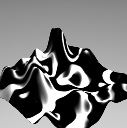
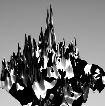
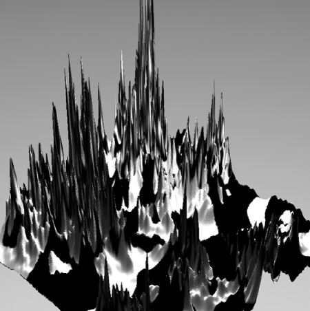
FIG. 3.: Evolution of scalar fields $\phi$ and $\Phi$ during the process of self-reproduction of the universe. The height of the distribution shows the value of the field $\phi$ which drives inflation. The surface is painted black in those parts of the universe where the scalar field $\Phi$ is in the first minimum of its effective potential, and white where it is in the second minimum. Laws of low-energy physics are different in the regions of different color. The peaks of the “mountains” correspond to places where quantum fluctuations bring the scalar fields back to the Planck density. Each of such places in a certain sense can be considered as a beginning of a new Big Bang.

VII Inflation and observations

Inflation is not just an interesting theory that can resolve many difficult problems of the standard Big Bang cosmology. This theory made several predictions which can be tested by cosmological observations. Here are the most important predictions:

1) The universe must be flat. In most models $\Omega_{total}=1\pm 10^{-4}$.

2) Perturbations of metric produced during inflation are adiabatic.

3) Inflationary perturbations have flat spectrum. In most inflationary models the spectral index $n=1\pm 0.2$ ($n=1$ means totally flat.)

4) These perturbations are gaussian.

5) Perturbations of metric could be scalar, vector or tensor. Inflation mostly produces scalar perturbations, but it also produces tensor perturbations with nearly flat spectrum, and it does not produce vector perturbations. There are certain relations between the properties of scalar and tensor perturbations produced by inflation.

6) Inflationary perturbations produce specific peaks in the spectrum of CMB radiation.

It is possible to violate each of these predictions if one makes this theory sufficiently complicated. For example, it is possible to produce vector perturbations of metric in the models where cosmic strings are produced at the end of inflation, which is the case in some versions of hybrid inflation. It is possible to have open or closed inflationary universe, it is possible to have models with nongaussian isocurvature fluctuations with a non-flat spectrum. However, it is extremely difficult to do so, and most of the inflationary models satisfy the simple rules given above.

It is not easy to test all of these predictions. The major breakthrough in this direction was achieved due to the recent measurements of the CMB anisotropy. These measurements revealed the existence of two (or perhaps even three) peaks in the CMB spectrum. Position of these peaks is consistent with predictions of the simplest inflationary models with adiabatic gaussian perturbations, with $\Omega=1\pm 0.03$, and $n=1.03\pm 0.06$ [30].

Inflationary scenario is very versatile, and now, after 20 years of persistent attempts of many physicists to propose an alternative to inflation, we still do not know any other way to construct a consistent cosmological theory. But may be we did not try hard enough?

Since most of inflationary models are based on 4D cosmology, it would be natural to venture into the study of higher-dimensional cosmological models. In what follows we will discuss one of the recent attempts to formulate an alternative cosmological scenario.

VIII Alternatives to inflation?

There were many attempts to suggest an alternative to inflation. However, in order to compete with inflation a new theory should offer an alternative solution to many difficult cosmological problems. Let us look at these problems again before starting a discussion.

1) Homogeneity problem. Before even starting investigation of density perturbations and structure formation, one should explain why the universe is nearly homogeneous on the horizon scale.

2) Isotropy problem. We need to understand why all directions in the universe are similar to each other, why there is no overall rotation of the universe. etc.

3) Horizon problem. This one is closely related to the homogeneity problem. If different parts of the universe have not been in a causal contact when the universe was born, why do they look so similar?

4) Flatness problem. Why $\Omega=1\pm 0.03$? Why parallel lines do not intersect?

5) Total entropy problem. The total entropy of the observable part of the universe is greater than $10^{87}$. Where did this huge number come from? Note that the lifetime of a closed universe filled with hot gas with total entropy $S$ is $S^{2/3}\times 10^{-43}$ seconds [14]. Thus $S$ must be huge. Why?

6) Total mass problem. The total mass of the observable part of the universe has mass $\sim 10^{60}M_{p}$. Note also that the lifetime of a closed universe filled with nonrelativistic particles of total mass $M$ is ${M\over M_{P}}\times 10^{-43}$ seconds. Thus $M$ must be huge. But why?

7) Structure formation problem. If we manage to explain the homogeneity of the universe, how can we explain the origin of inhomogeneities required for the large scale structure formation?

8) Monopole problem, gravitino problem, etc.

This list is very long. That is why it was not easy to propose any alternative to inflation even before we learned that $\Omega\approx 1$, $n\approx 1$, and that the perturbations responsible for galaxy formation are mostly adiabatic, in agreement with predictions of the simplest inflationary models.

Despite this difficulty (or maybe because of it) there was always a tendency to announce that we have eventually found a good alternative to inflation. This was the ideology of the models of structure formation due to topological defects or textures. Of course, even 10 years ago everybody knew that these theories at best could solve only one problem (structure formation) out of the 8 problems mentioned above. The true question was whether inflation with cosmic strings/textures is any better than inflation without cosmic strings/textures. However, such a formulation would not make the headlines. Therefore the models of structure formation due to topological defects or textures sometimes were advertised in public press as the models that “match the explanatory triumphs of inflation while rectifying its major failings” [31].

Recently the theory of topological defects and textures as a source of the large scale structure was essentially ruled out by observational data, but the tradition of advertisement of various ‘successful’ alternatives to inflation is still flourishing. Recent example is given by the ekpyrotic/cyclic scenario [32, 33]. The 50-pages long paper on ekpyrotic scenario [32] appeared in hep-th in April 2001, and ten days later, before any experts could make their judgement, it was already enthusiastically discussed on BBC and CNN as a viable alternative to inflation. The reasons for the enthusiasm can be easily understood. We were told that finally we have a cosmological theory that is based on string theory and that is capable of solving all major cosmological problems without any use of inflation, which was called ‘superluminal expansion’ [32].

However, a first look at this scenario revealed several minor problems and inconsistencies, then we have found much more serious problems, and eventually it became apparent that the original version of the ekpyrotic scenario [32] did not live to its promise [34, 35]. In particular, instead of expanding, the ekpyrotic universe collapses to a singularity [35, 36]. The theory of density perturbations in this scenario is very controversial [37, 38, 39, 40, 41, 42]. More importantly, this scenario offers no solution to major cosmological problems such as the homogeneity, flatness and entropy problems, so it is not a viable alternative to inflation [34]. Let me explain this part first, before we turn our attention to the cyclic scenario [33].

IX Ekpyrosis

A Basic scenario

According to the ekpyrotic scenario [32], we live at one of the two ‘heavy’ 4D branes in 5D universe described by the Hor̆ava-Witten (HW) theory [43]. Our brane is called visible, and the second brane is called hidden. There is also a ‘light’ bulk brane at a distance $Y$ from the visible brane in the 5th direction.

The three brane configuration is assumed to be in a nearly stable BPS state. The bulk brane has potential energy $V(Y)=-ve^{-m\alpha Y}$, where $m$ is some constant. It is assumed that at small $Y$ the potential suddenly vanishes.

The bulk brane moves towards our brane and collides with it. Due to the slight contraction of the scale factor of the universe, the bulk brane carries some residual kinetic energy immediately before the collision with the visible brane. After the collision, this residual kinetic energy transforms into radiation which will be deposited in the three dimensional space of the visible brane. The visible brane, now filled with hot radiation, somehow begins to expand as a flat FRW universe. Quantum fluctuations of the position of the bulk brane generated during its motion from $Y=R$ to $Y=0$ will result in density fluctuations with a nearly flat spectrum. The spectrum will have a blue tilt. It is argued that the problems of homogeneity, isotropy, flatness and horizon do not appear it this model because the universe, according to [32], initially was in a nearly BPS state, which is homogeneous.

B Ekpyrotic scenario versus string theory

It would be great to have a realistic brane cosmology based on string theory. However, ekpyrotic theory is just one of the many attempts to do so, and its relation to string theory is rather indirect.

One of the central assumptions of the ekpyrotic scenario is that we live on a negative tension brane. However, the standard HW phenomenology [43] is based on the assumption that the tension of the visible brane is positive. There were two main reasons for such an assumption. First of all, in practically all known versions of the HW phenomenology, with few exceptions, a smaller group of symmetry (such as $E_{6}$) lives on the positive tension brane and provides the basis for GUTs, whereas the symmetry $E_{8}$ on the negative tension brane may remain unbroken. It is very difficult to find models where $E_{6}$ or $SU(5)$ live on the negative tension brane [44, 45].

There is another reason why the tension of the visible brane is positive in the standard HW phenomenology [43]: The square of the gauge coupling constant is inversely proportional to the Calabi-Yau volume [43]. On the negative tension brane this volume is greater than on the positive tension one, see e.g. [32]. In the standard HW phenomenology it is usually assumed that we live on the positive tension brane with small gauge coupling, ${g^{2}_{GUT}\over 4\pi}\sim 0.04$. On the hidden brane with negative tension the gauge coupling constant becomes large, ${g^{2}_{hidden}\over 4\pi}=O(1)$, which makes the gaugino condensation possible [43]. It is not impossible to have a consistent phenomenology with the small gauge coupling on the hidden brane, but this is an unconventional and not well explored possibility [44]. Therefore the original version of the ekpyrotic scenario was at odds with the standard HW phenomenology as defined in [43].

Another set of problems is related to the potential $V(Y)$ playing crucial role in this scenario. This potential is supposed to appear as a result of nonperturbative effects. However, it is not clear whether the potential with required properties may actually emerge in the HW theory. Indeed, the potential $V(Y)$ must be very specific. It should vanish at $Y=0$, and it must be negative and behave as $-e^{-\alpha mY}$ at large $Y$. One could expect terms like that, but in general one also obtains terms such as $\pm e^{-\alpha m(R-Y)}$, where $R-Y$ is the distance between the bulk brane and the second ‘heavy’ brane  [46]. Such terms, as well as power-law corrections, must be forbidden if one wants to obtain density perturbations with flat spectrum [34]. The only example of a calculation of the potential of such type was given in [46]. In this example the “forbidden” terms $\pm e^{-\alpha m(R-Y)}$ do appear, and the sum of all terms is not negative, as assumed in [32], but strictly positive [46].

An additional important condition is that near the hidden brane the absolute value of the potential must be smaller than $e^{-120}$, because otherwise the density perturbations on the scale of the observable part of the universe will not be generated [34]. Also, if one adds a positive constant suppressed by the factor $\sim e^{-120}$ to $V(Y)$, inflation may begin. This is something the authors of the ekpyrotic scenario were trying to avoid.

But if the nonperturbative effects responsible for $V(Y)$ are so weak, how can they compete with the strong forces which are supposed to stabilize the positions of the visible brane and the hidden brane in Hor̆ava-Witten theory? Until the brane stabilization mechanism is understood, it is very hard to trust any kind of “derivation” of the miniscule nonperturbative potential $V(Y)$ with extremely fine-tuned properties.

After we made these comments [34], the authors of the ekpyrotic scenario have changed it. In the cyclic scenario [33] the potential $V(Y)$ is supposed to approach a small positive value at large $Y$. This leads to inflation that is supposed to solve the homogeneity problem. Thus, cyclic scenario is no longer an alternative to inflation. Also, the branes in cyclic scenario are not stabilized. Therefore this scenario is no longer related to the standard string phenomenology.

C Singularity problem

The discussion of brane collision in the ekpyrotic scenario was based on static 5D solution describing non-moving branes in the absence of the potential $V(Y)$ [32]. However, the action as well as the solution for the static 3-brane configuration given in [32] was not quite correct. The corrected version of the action and the solution was given in  [35].

More importantly, the solution discussed there was given for branes that were not moving. It was assumed in [32] that in order to study 5D cosmological solutions it is sufficient to take the static metric used in [32] and make its coefficients time-dependent. However, we have found that the 5D cosmological solution given in [32] was incorrect. The ansatz for the metric and the fields used in [32] does not solve the time-dependent 5D equations [35]. Moreover, we have shown that if one uses effective 4D theory in order to describe the brane motion, as proposed in [32], the universe after the brane collision can only collapse  [35]. Thus, instead of the Big Bang one gets a Big Crunch! This conclusion later was confirmed in [36].

Since that time, the singularity problem became an unavoidable part of the ekpyrotic/cyclic scenario. This problem is very complicated. In this respect, various authors have rather different opinions. Those who ever tried to solve this problem in general relativity are more than skeptical. The authors of the ekpyrotic scenario hope that experts in string theory will solve the problem of the cosmological singularity very soon. Meanwhile, the experts in string theory study toy models, such as the 2+1 dimensional model with a null singularity rather than with a space-like cosmological singularity [48]. Even in these models the situation is very complicated because of certain divergent scattering amplitudes. Therefore at present string theorists do not want to make any speculations about the resolution of the singularity problem in realistic cosmological theories [49, 50].

D Density perturbations

The problems discussed above are extremely complicated. But let us take a positive attitude and assume for a moment that all of these problems eventually will be solved.

Now let us discuss the mechanism of generation of density perturbations in the ekpyrotic scenario. As was shown in [34], this mechanism is based on the tachyonic instability with respect to generation of quantum fluctuations of the bulk brane position in the theory with the potential $V(Y)\sim-e^{-\alpha mY}$. One may represent the position of the brane $Y(x)$ by a scalar field $\phi$, and find that the long wavelength quantum fluctuations of this field grow exponentially because the effective mass squared of this field, proportional to $V^{\prime\prime}(Y)$, is negative. A detailed theory of such instabilities recently was developed in the context of the theory of tachyonic preheating [19].

Inhomogeneities of the brane position lead to the $x$-dependent time delay of the Big Crunch, i.e. of the moment when the ‘brane damage’ occurs and matter is created. In inflationary theory, a position-dependent delay of the moment of reheating leads to density perturbations [9, 10]. Simple estimates based on a similar idea lead to the conclusion [34] that in the scenario with $V(Y)\sim-e^{-\alpha mY}$ one obtains a nearly flat spectrum of perturbations $\delta t$. If one naively multiplies $\delta t$ by $H$ after the brane collision, these perturbations translate into density perturbations $\delta\rho/\rho\sim H\delta t$. These perturbations have flat spectrum with a small red tilt [34].

However, this approach is oversimplified. Just as in the case of inflationary theory, one should specify when the Hubble constant is to be evaluated. In the ekpyrotic theory this question is crucial, because during the process of production of the perturbations $\delta t$ the Hubble constant is vanishingly small, and it was rapidly changing. Therefore if one multiplies $\delta t$ by $H$ at the time of the production of fluctuations $\delta\phi$, as we did for inflationary theory, one will get extremely small perturbations with a non-flat spectrum.

In order to obtain an unambiguous result, one should use the methods developed in [11]. There were several attempts to do so. The authors of the ekpyrotic theory, as usual, are very optimistic and claim that they are obtaining perturbations with flat spectrum [37]. Meanwhile everybody else [38, 39, 40, 41], with exception of Ref. [42], insist that adiabatic perturbations with flat spectrum are not generated in this scenario, or, in the best case, we simply cannot tell anything until the singularity problem in this theory is resolved.

I share this point of view, and I would like to add to it something else. The theory of density perturbations in the ekpyrotic/cyclic scenario is immensely complicated. The authors of [37] have already made 3 revisions of their paper, and the final results continue slightly changing. Whereas originally the spectrum of perturbations in their scenario was supposed to be blue (decreasing at large scales) [32], now they say that it is red. In order to obtain perturbations of desirable magnitude, it is usually required that the absolute value of the effective potential $V(Y)$ should be greater than the Planck density, $|V(Y)|\gtrsim 1$ [37, 33], see below. But in this case the perturbation theory is expected to fail, quite independently of the singularity problem.

I believe that a complete analysis of this problem could be possible only in the 5D theory rather than in the effective 4D theory. This brings additional complications described in [35, 51].

E And the main problem is…

If adiabatic density perturbations with flat spectrum are not produced [38, 39, 40, 41], one may stop any further discussion of this scenario. However, let us be optimistic again and assume that the singularity problem is resolved and the theory of density perturbations developed in [32, 34, 37] is correct. In this case one has a new problem to consider.

Tachyonic instability, which is the source of these perturbations, amplifies not only quantum fluctuations, but also classical inhomogeneities [34]. These inhomogeneities grow in exactly the same way as the quantum fluctuations with the same wavelength. Therefore to avoid cosmological problems the initial classical inhomogeneities of the branes must be below the level of quantum fluctuations. In other words, the universe on the large scale must be ideally homogeneous from the very beginning. By evaluating the initial amplitude of quantum fluctuations on the scale corresponding to the observable part of the universe one finds that the branes must be parallel to each other with an accuracy better than $10^{-60}$ on a scale $10^{30}$ times greater than the distance between the branes [34].

To understand the nature of the problem one may compare this scenario with inflation. Inflation removes all previously existing inhomogeneities and simultaneously produces small density perturbations. Meanwhile in the ekpyrotic scenario even very small initial inhomogeneities become exponentially large. Therefore instead of resolving the homogeneity problem, the ekpyrotic scenario makes this problem much worse.

Now let us assume for a moment that we were able to solve the homogeneity problem without using inflation. But we still have the flatness/entropy problem to solve. Suppose that the universe is closed, and initially it was filled with radiation with total entropy $S$. Then its total lifetime is given by $t\sim S^{2/3}M_{p}^{-1}$, after which it collapses [14]. In order to survive until the moment $t\sim 10^{34}M_{p}$, where the inhomogeneities on the scale of the present horizon are produced in the ekpyrotic scenario, the universe must have the total entropy greater than $10^{50}$ [34]. Thus in order to explain why the total entropy (or the total number of particles) in the observable part of the universe is greater than $10^{88}$ one must assume that it was greater than $10^{50}$ from the very beginning. This is the entropy problem [14]. If the universe initially has the Planckian temperature, its total initial mass must be greater than $10^{50}M_{p}$, which is the mass problem. Also, such a universe must have very large size from the very beginning, which is the essence of the flatness problem [14].

In comparison, in the simplest versions of chaotic inflation scenario the homogeneity problem is solved if our part of the universe initially was relatively homogeneous on the smallest possible scale $O(M_{p}^{-1})$ [13]. The whole universe could have originated from a domain with total entropy $O(1)$ and total mass $O(M_{p})$. Once this process begins, it leads to eternal self-reproduction of the universe in all its possible forms [21, 14]. Nothing like that is possible in the ekpyrotic scenario.

Thus, the original version of the ekpyrotic scenario does not represent a viable alternative to inflation. Independently of all other troublesome features of the ekpyrotic scenario, it does not solve the homogeneity, flatness and entropy problems. Apparently, the authors of this scenario realized it, because their new model, cyclic scenario [33], includes an infinite number of stages of inflation. Each new stage of inflation is supposed to ensure homogeneity of the universe at the subsequent cycle. The main difference between this version of inflationary theory and the usual one is that inflation in cyclic universe occurs before the singularity rather than immediately after it. I will describe this scenario following our recent paper with Felder, Frolov and Kofman [52].

X Cyclic universe

A Basic scenario

In Ref. [34] it was pointed out that avoiding inflation in the ekpyrotic scenario requires incredible fine-tuning. If one adds a small positive constant $V_{0}$ to $V(Y)\sim-e^{-\alpha mY}$, the universe at large $Y$ becomes inflationary. In the beginning the authors of the ekpyrotic scenario claimed that they do not need this stage of ‘superluminal expansion’ to solve all major cosmological problems, but eventually they did exactly what we suggested in [34]: They added a small constant $V_{0}\sim 10^{-120}$ (in Planck units) to $V(Y)\sim-e^{-\alpha mY}$, which leads to inflation at large $Y$.

Since the cyclic scenario is formulated mainly in terms of the effective 4D theory with the brane separation $Y$ represented by a scalar field $\phi$, we will follow the same route. In this language, cyclic scenario, unlike ekpyrotic scenario, assumes, in accordance with [34], that the potential $V(\phi)$ at large $\phi$ behaves as $V_{0}(1-e^{-c\phi})$ [33]:

$$V(\phi)=V_{0}~{}(1-e^{-c\phi})~{}F(\phi)\ .$$ (11)

In the particular example studied in the last paper of Ref. [33] one has $F(\phi)=e^{-e^{-\gamma\phi}}$, $V_{0}=10^{-120}$, $c=10$, $\gamma\approx 1/8$. This potential is shown in Fig. 4. At $\phi=0$ this potential vanishes. It approaches its asymptotic value $V_{0}=10^{-120}$ at $\phi\gtrsim 1$.

FIG. 4.: Cyclic scenario potential used in Ref. [33]. The potential at $\phi>1$ approaches a very small constant value $V_{0}\sim 10^{-120}$. At $\phi\ll-40$ the potential vanishes.

Inflation in this scenario is possible at $\phi\gtrsim 1$. The potential has a minimum at $\phi\approx-36$; the value of the potential in this minimum is $V_{\rm min}\approx-3$ in units of Planck density [33].

Let us try to understand the origin of the parameters $c=10$, $\gamma\approx 1/8$ and $V_{\rm min}\sim 3$ used in [33]. According to [37], the amplitude of density perturbations can be estimated as ${\delta_{H}}\lesssim 10^{-7}\xi^{4}v_{0}^{-2/3}\sqrt{|V_{\rm min}|}$. Here $\xi\ll 1$ and $v_{0}$ is a ratio of Calabi-Yau volume to $M_{GUT}^{-6}$. That is why in order to obtain ${\delta_{H}}\sim 2\times 10^{-5}$ for $v_{0}=O(1)$ [53] one should have $|V_{\rm min}|\gg 1$. The spectrum of density perturbations obtained in [37] is not blue, as in [32], but red, like in the simplest versions of chaotic inflation. The spectral index is $n\approx 1-4/c^{2}$. Observational data suggest that $n=1.03\pm 0.06$ [30], which implies that $c\gtrsim 10$. If one takes $c\gg 10$, and $V_{\rm min}>1$, one finds that the curvature of the effective potential in its minimum becomes much greater than 1, i.e. the scalar particles there have mass that is much greater than $M_{p}$.

Once one takes $V\sim-3$ in the minimum of the potential with $c=10$ [33], the parameter $\gamma$ can be determined numerically: $\gamma=0.1226$. It would be hard to provide explanation of the numerical value of this parameter. If one takes, for example, $\gamma=1/8=0.125$, one finds $V\sim-3\times 10^{-3}$ in the minimum of the potential. This would reduce ${\delta_{H}}$ by a factor of 30. Thus, in order to have density perturbations with a correct magnitude one should fine-tune the value of $\gamma=0.1226$ with accuracy better than 1%.

According to cyclic scenario, right now the scalar field is large, $\phi>1$, so that $V(\phi)\approx V_{0}\sim 10^{-120}$. This corresponds to the present stage of accelerated expansion of the universe. Gradually the field $\phi$ begins drifting to the left and falls towards the minimum of $V(\phi)$. On the way there the curvature of the potential becomes negative, and therefore small perturbations of the field $\phi$ are generated by the mechanism explained in [19, 32, 34]. These are the fluctuations that are supposed to produce density perturbations after the singularity.

Then the field reaches the region with $V(\phi)<0$. At some point the total energy (including kinetic energy) vanishes. At that time, according to the Friedmann equation for a flat universe ${\dot{a}^{2}/a^{2}}=\rho/3$, the universe stops expanding and begins to contract to a singularity. Collapse leads to negative friction coefficient $3H$ in the term $3H\dot{\phi}$, which accelerates the evolution of the field $\phi$. A numerical investigation of the motion of the field moving from $\phi>0$ in a theory with this potential shows that its kinetic energy at the moment when $\phi$ reaches the minimum of the effective potential is $O(10^{2})M_{p}^{4}$. When the field approaches $\phi\sim-39$, where the effective potential becomes flat, the kinetic energy of the field $\phi$ becomes $\sim 10^{6}M_{p}^{4}$, i.e. a million times greater than the Planck density!

At this stage a weaker soul could falter, but we must proceed because we did not describe the complete scenario yet.

The subsequent evolution develops very fast. When the field accelerates enough it enters the regime $\dot{\phi}^{2}\gg V(\phi)$ and continues moving to $-\infty$ with a speed practically independent of $V(\phi)$: $\phi\sim\ln t$, $\dot{\phi}\sim t^{-1}$, where $t$ is the time remaining until the Big Crunch singularity. For all potentials $V(\phi)$ growing at large $\phi$ no faster than some power of $\phi$ one has $\dot{\phi}^{2}/2$ growing much faster than $V(\phi)$ (a power law singularity versus a logarithmic singularity). This means that one can neglect $V(\phi)$ in the investigation of the singularity, virtually independently of the choice of the potential at large $|\phi|$ [52]. This regime corresponds to a ‘stiff’ equation of state $p=\rho$.

Usually, the Big Crunch singularity is considered the end of the evolution of the universe. However, in the cyclic scenario it is assumed that the universe goes through the singularity and re-appears again. When it appears, in the first approximation it looks exactly as it was before, and the scalar field moves back exactly by the same trajectory by which it reached the singularity [50].

This is not a desirable cyclic regime. Therefore it is assumed in [33] that the value of kinetic energy of the field $\phi$ increases after the bounce from the singularity. This increase of energy of the scalar field is supposed to appear as a result of particle production at the moment of the brane collision (even though one could argue that usually particle production leads to an opposite effect). It is very hard to verify the validity of this crucial assumption since the consistency of the 5D picture proposed in [33] is questionable, see e.g. [51]. But let us just assume that this is indeed the case because otherwise the whole scenario does not work and we have nothing to discuss. If the increase of the kinetic energy is large enough, the field $\phi$ rapidly rolls over the minimum of $V(\phi)$ in a state with a positive total energy density, and continues its motion towards $\phi>0$. The kinetic energy of the field decreases faster than the energy of matter produced at the singularity. At some moment the energy of matter begins to dominate. Eventually the energy density of ordinary matter becomes smaller than $V(\phi)$ and the present stage of inflation (acceleration of the universe) starts again. This happens if the field $\phi$ initially moved fast enough to reach the plateau of the effective potential at $\phi\gg 1$.

Because the potential at $\phi\gg 1$ is very flat, the field may stay there for a long time and inflation will make the universe flat and empty. Eventually the field rolls towards the minimum of the potential again, and the universe enters a new cycle of contraction and expansion.

As we see, this version of the ekpyrotic scenario is not an alternative to inflation anymore. Rather it is a very specific version of inflationary theory. The major cosmological problems are supposed to be solved due to exponential expansion in a vacuum-like state, i.e. by inflation, even though it is a low-energy inflation and the mechanism of production of density perturbations in this scenario is non-standard. Let us remember that Guth’s first paper on inflation [3] was greeted with so much enthusiasm precisely because it proposed a solution to the homogeneity, isotropy, flatness and horizon problems due to exponential expansion in a vacuum-like state, even though it didn’t address the formation of large scale structure. The Starobinsky model that was proposed a year earlier [15] could account for large scale structure and the observed CMB anisotropy [9], but it did not attract as much attention because it did not address the possibility of solving these initial condition problems.

In fact, the stage of acceleration of the universe in the cyclic model is eternal inflation. Eternal inflation occurs if $V^{\prime 2}\ll V^{3}$ [21, 28]. For the potential $V(\phi)$ used in the cyclic model this condition is satisfied at large $\phi$ since $V=const$ in the limit $\phi\to\infty$, whereas $V^{\prime}\to 0$ in this limit. Thus the universe at large $\phi$ (at $\phi>15$ in the model of Ref. [33]) enters the stage of eternal self-reproduction, quite independently of the possibility to go through the singularity and re-appear again. In other words, the universe in the cyclic scenario is not merely a chain of eternal repetition, as expected in [33], but a growing self-reproducing inflationary fractal of the type discussed in [27, 21, 28].

One may wonder, however, whether this version of inflationary theory is good enough to solve all major cosmological problems. Indeed, inflation in this scenario may occur only at a density 120 orders of magnitude smaller than the Planck density. If, for example, one considers a closed universe filled with matter and a scalar field with the potential used in the cyclic model, it will typically collapse within the Planck time $t\sim 1$, so it will not survive until the beginning of inflation in this model at $t\sim 10^{60}$. For consistency of this scenario, the overall size of the universe at the Planck time must be greater than $l\sim 10^{30}$ in Planck units, which constitutes the usual flatness problem. The total entropy of a hot universe that may survive until the beginning of inflation at $V\sim 10^{-120}$ should be greater than $10^{90}$, which is the entropy problem [14]. An estimate of the probability of quantum creation of such a universe “from nothing” gives $P\sim e^{-|S|}\sim\exp\left(-{24\pi\over V_{0}}\right)\sim e^{-120}$ [54].

There are many other unsolved problems related to this theory, such as the origin of the potential $V(\phi)$ [34] and the 5D description of the process of brane motion and collision [35, 51]. In particular, the cyclic scenario assumes that the distance between the branes is not stabilized, i.e. the field $\phi$ at present is nearly massless. This may lead to a strong violation of the equivalence principle. This is one of the main reasons why it is usually assumed that the branes in Hor̆ava-Witten theory must be stabilized. To avoid this problem, the authors of [33] introduce the function $\beta(\phi)$ describing interaction of the scalar field with matter. The violation of the equivalence principle can be avoided if $(\ln\beta(\phi))_{,\phi}\ll 10^{-3}$. However, in the Kaluza-Klein limit, in which the 4D approximation used in [33] could be valid, one has $\beta(\phi)\sim e^{\phi/\sqrt{6}}$ [33]. In this approximation, one has $(\ln\beta(\phi))_{,\phi}=1/\sqrt{6}$, and the equivalence principle is strongly violated.

We will not discuss these problems here any longer. Instead of that, we will concentrate on the phenomenological description of possible cycles using the effective 4D description of this scenario. This will allow us to find out whether the cyclic regime is indeed a natural feature of the scenario proposed in [33].

B Are there any cycles in the cyclic scenario?

As we have seen, the existence of the cyclic regime requires investigation of particle production in the singularity. Fortunately, this subject was intensely studied more than 20 years ago. The main results can be summarised as follows. Since $H\sim t^{-1}$ in the standard big bang theory, the curvature scalar $R$ in the universe dominated by a kinetic energy of a scalar field behaves as $t^{-2}$ . Scalar particles minimally coupled to gravity, as well as gravitons and helicity 1/2 gravitinos [55], are not conformally invariant; their frequencies thus experience rapid nonadiabatic changes induced by the changing curvature. These changes lead to particle production due to nonadiabaticity with typical momenta $k^{2}\sim R\sim t^{-2}$. The total energy-momentum tensor of such particles produced at a time $t$ after (or before) the singularity is $T_{\mu\nu}\sim O(k^{4})\sim R^{2}\sim t^{-4}$ [56, 57]. Comparing the density of produced particles with the classical matter or radiation density of the universe $\rho\sim t^{-2}$, one finds that the density of created particles produced at the Planck time $t\sim 1$ is of the same order as the total energy density in the universe. Moreover, if one bravely attempts to describe the situation near the singularity, at $R>1$, then one may conclude that the contribution of particles produced near the singularity (as well as the contribution of quantum corrections to $T_{\mu\nu}$) is always greater than the energy momentum tensor of the classical scalar field.

This argument will be very important for us. The existence of even a small amount of particles created near the singularity may have a significant effect on the motion of the field. Indeed, the kinetic energy of the scalar field $\dot{\phi}^{2}/2$ in the regime $\dot{\phi}^{2}/2\gg V(\phi)$ decreases as $a^{-6}$. Meanwhile, the density of ultrarelativistic particles decreases as $a^{-4}$. Therefore at some moment $t_{0}$ the energy density of ultrarelativistic particles eventually becomes greater than $\dot{\phi}^{2}/2$. In this regime (and neglecting $V(\phi)$) one can show that $\dot{\phi}=\dot{\phi}_{0}{a_{0}^{3}\over a^{3}}=\dot{\phi}_{0}\left({t_{0}\over t}\right)^{3/2}$. Even if this regime continues for an indefinitely long time, the total change of the field $\phi$ during this time remains quite limited. Indeed,

$$\Delta\phi\leq\int\limits_{t_{0}}^{\infty}\dot{\phi}dt=\dot{\phi}_{0}\int\limits_{t_{0}}^{\infty}\left({t_{0}\over t}\right)^{3\over 2}dt=2~{}\dot{\phi}_{0}t_{0}.$$ (12)

If $t_{0}$ is the very beginning of radiation domination ($\dot{\phi}_{0}^{2}/2\sim\rho_{\rm total}$), then $H_{0}\sim t_{0}^{-1}\sim\dot{\phi}_{0}$. Therefore

$$\Delta\phi\lesssim 1$$ (13)

in Planck units (i.e. $\Delta\phi\lesssim M_{p}$).

This simple result has several important implications. In particular, if the motion of the field in a matter-dominated universe begins at $|\phi|\gg 1$, then it can move only by $\Delta\phi\lesssim 1$. Therefore in theories with flat potentials the field always remains frozen at $|\phi|\gg 1$. It begins moving again only when the Hubble constant decreases and $|3H\dot{\phi}|$ becomes comparable to $|V,_{\phi}|$. But in this case the condition $3H\dot{\phi}\approx|V,_{\phi}|$ automatically leads to inflation in such theories as $m^{2}\phi^{2}/2$ for $\phi\gg 1$. This means that even a small amount of matter or radiation may increase the chances of reaching a stage of inflation, see [58, 52].

In application to the cyclic scenario this result implies that the scalar field in presence of ultrarelativistic matter created near the singularity should immediately loose its kinetic energy and freeze to the left of the minimum of the effective potential at Fig. 4. Then it slowly falls to the minimum. If the field would move rapidly, as expected in [33] , it would roll to positive $\phi$ without triggering the collapse of the universe. But a slow motion leads to a collapse of the universe [52], instead of the inflationary stage anticipated in [33].

But what if we are wrong, and for some reason particle production near the singularity was inefficient [59]? Independently of it, a later stage of efficient particle production is unavoidable. Indeed, at $\phi<-40$ the mass squared of the scalar field $m^{2}=V^{\prime\prime}$ vanishes. Near the minimum one has $m\gtrsim O(1)$ in Planck units, and at $\phi>-32$ the mass almost exactly vanishes again. The transition from $m\ll 1$ to $m\sim 1$ and back to $m\ll 1$ occurs within the time $\Delta t\sim 1$. Thus, the change of the mass was strongly non-adiabatic, with typical frequency $\sim 1$. This should lead to production of ultrarelativistic particles $\phi$ with Planckian density [18]. These particles, in their turn, should immediately freeze the motion of the field $\phi$ near $\phi\sim-30$. The field never reaches the region $\phi>1$, and inflation never begins. Instead of that, the field again slowly falls to the minimum of $V(\phi)$ and the universe collapses.

Thus, unless one makes some substantial modification to the scenario proposed in [33], it does not work in the way anticipated by its authors.

C Cycles and epicycles

Of course, one could save this scenario by adding new epicycles to it. For example, if particle production near the singularity at $\phi=-\infty$ freezes the field to the left of the minimum of $V(\phi)$, then the universe collapses for the second time when the field runs to $\phi=+\infty$. If the field bounces back from the singularity at $\phi=+\infty$ and then freezes at $\phi>0$ due to efficient particle production at the singularity, a stage of low-energy inflation begins. This scenario is quite different from the one proposed in [33], but it might work. Density perturbations in this scenario will be produced due to tachyonic instability in the potential with the shape determined by the term $e^{-e^{-\gamma\phi}}$.

Also, one may consider effects related to non-relativistic particles produced at the singularity. These particles contribute to the equation of motion for the field $\phi$ by effectively increasing its potential energy density [33]. They may push the field towards positive values of the field $\phi$ despite the effects described above. However, this would add an additional complicated feature to a scenario that is already quite speculative.

But one can do something simpler. For example, instead of the asymmetric potential shown in Fig. 4, one may consider a symmetric potential, as in Fig. 5. As a toy model, one may consider, e.g., a potential $V(\phi)=V_{0}(1-A\cosh^{-1}(\phi-\phi_{0}))$, where $A>1$ and $\phi_{0}$ are some constants.

FIG. 5.: Symmetric scalar field potential in the bicycling scenario. At large values of $|\phi|$ one has $V(\phi)\approx V_{0}\sim 10^{-120}$ and there is a minimum at $\phi=\phi_{0}$.

In the beginning, the scalar field is large and positive and it slowly moves towards the minimum. When it falls to the minimum the universe begins to contract and the field is rapidly accelerated towards the singularity at $\phi=-\infty$. As we already mentioned, the structure of the singularity is not sensitive to the existence of the potential, especially if it is as small as $V_{0}\sim 10^{-120}$.

Now let us assume, as in [33], that the field $\phi$ bounces from the singularity and moves back. The kinetic energy of the field rapidly drops down because of radiation, so it freezes at the plateau to the left of the minimum of $V(\phi)$. At this stage the energy density is dominated by particles produced near the singularity. Then the universe cools down while the field is still large and negative and the late-time stage of inflation begins. During this stage the field slowly slides towards the minimum of the effective potential and then rolls towards the singularity at $\phi\to\infty$. When it bounces from the singularity, a new stage of inflation begins. The universe in this scenario enters a cyclic regime with twice as many cycles as in the original cyclic scenario of Ref. [33]. The same regime will appear even if the potential is asymmetric but positive both at $\phi\ll 0$ and at $\phi\gg 0$. We have called it the bicycling scenario [52].

An advantage of this scenario is that it may work even if, as we expect, a lot of radiation is produced at the singularity and the field $\phi$ rapidly loses its kinetic energy. However, if in order to have density perturbations of a sufficiently large magnitude one needs to have a potential with a super-Planckian depth $V(\phi)<-1$, as in [37, 33], then this scenario has the same problem as the scenario considered in the previous section. The kinetic energy of the field $\phi$ becomes greater than the Planck density as soon as it rolls to the minimum of $V(\phi)$. It becomes even much greater when the field rolls out of the minimum, and the 4D description fails.

Thus, bicycling scenario is more robust than the original version of the cyclic scenario [33], but it is still very problematic.

D Cycles with inflationary density perturbations

Even though it may not be easy to solve the singularity problem, the old idea that the big bang is not the beginning of the universe but a point of a phase transition is quite interesting, see e.g. [60]-[67]. However, the more assumptions about the singularity one needs to make, the less trustworthy are the conclusions. In this respect, inflationary theory provides us with a unique possibility to construct a theory largely independent of any assumptions about the initial singularity. According to this theory, the structure of the observable part of the universe is determined by processes at the last stages of inflation, at densities much smaller than the Planck density. As a result, observational data practically do not depend on the unknown initial conditions in the early universe.

But this very fact puts all theories of passing through the singularity in a difficult position. Indeed, one could argue that if the universe passes through the singularity, but afterwards there is a stage of inflation that erases all observational consequences of this event, then why bother? That is why some authors were trying to avoid having inflation after the singularity.

In my opinion, the possibility that the universe may pass through the cosmological singularity is extremely interesting independently of absence or presence of any observational consequences of this event. We need to have a consistent cosmological theory, including all possible stages of the evolution of the universe, whether they are accessible to observations or not.

An interesting attempt to construct such a theory was made in the context of the Pre-Big Bang scenario [67]. The main idea of this theory is extremely attractive. However, the authors of the PBB scenario decided to consider only those versions of the theory that do not have inflation after the singularity. As a result, in addition to the unsolved singularity problem, the PBB theory has a problem with production of adiabatic density perturbations with flat spectrum. More importantly, without help of inflation the PBB theory does not solve the homogeneity, isotropy, flatness and entropy problems [68]. So why do not we add a stage of inflation after the singularity? Of course, this would make the passage through the singularity irrelevant from the point of view of observations. However, this would solve the major cosmological problems (if the singularity problem is solved) and make the whole scenario, including the non-trivial stage of the pre-big bang evolution, consistent with observational data.

The situation with the cyclic scenario is very similar. I believe that the necessity to solve the singularity problem and to know exactly what happens with small density perturbations at the singularity is a significant step back from the simple picture provided by the usual versions of inflationary theory. Since the cyclic scenario does require repeated periods of inflation anyway, it would be nice to avoid the vulnerability of this scenario with respect to the unknown physics at the singularity by placing the stage of inflation before the stage of large scale structure formation rather than after it.

In order to do it [52], one may consider a toy model with a potential

$$V(\phi) = V_{0}(1-A\cosh^{-1}(\phi-\phi_{0}))\qquad{\rm for}~{}~{}\phi<0\ ,$$ (14)

$$V(\phi) = V_{0}(1-A\cosh^{-1}(\phi-\phi_{0}))+{m^{2}\over 2}\phi^{2}~{}~{}{\rm for}~{}~{}\phi>0\ .$$ (15)

Thus, for $m=0$ this is the same potential as in the bicycling scenario proposed in the previous section. If one takes $\phi_{0}\ll-1$, then the potential at $\phi<0$ looks very similar to the potential of the original cyclic model, see Fig. 4, but it is positive everywhere except a small vicinity of $\phi_{0}$, see Fig. 6. Also, we will not need to have a very deep minimum of the effective potential because density perturbations will be produced by the standard inflationary mechanism. Therefore one can take $A$ just a bit greater than 1. At $\phi>0$ the potential coincides with the simplest chaotic inflation potential $V_{0}+{m^{2}\over 2}\phi^{2}$ considered in the beginning of this paper.

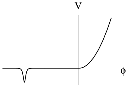
FIG. 6.: Scalar field potential in the cyclic scenario incorporating a stage of chaotic inflation. The potential has a minimum at $\phi_{0}<0$. Inflationary perturbations are generated and the large-scale structure of the universe is produced at $\phi>0$.

Now let us assume that initially the universe was slowly inflating in a state with $\phi<\phi_{0}$. Then the scalar field started moving towards the minimum of the effective potential, as in the cyclic scenario (though in an opposite direction). When the field approaches the minimum, the universe begins to collapse. After that moment, the field begins growing with an increasing speed. Let us assume that one can ignore the effective potential ${m^{2}\over 2}\phi^{2}$ that appears only at $\phi>0$. According to the investigation performed in [52], for $A=O(1)$ the kinetic energy of the field $\phi$ will reach the Planck value $\dot{\phi}^{2}/2\sim 1$ at $\phi-\phi_{0}\sim 100$. Meanwhile, for $m=3\times 10^{-6}$ (COBE normalization), the effective potential ${m^{2}\over 2}\phi^{2}$ reaches the Planck value only at $\phi\sim 10^{5}$, where the kinetic energy of the field $\phi$ would be much greater than 1. Thus, if one takes $A=O(1)$, $\phi_{0}\sim 100$, one can completely ignore $V(\phi)$ during the investigation of the development of the singularity, as well as during the first stages of the motion of the field $\phi$ bounced back from $+\infty$.

However, according to our discussion of particle production and their effect on the motion of the scalar field, one may expect that after bouncing from the singularity the scalar field immediately freezes and does not move (or moves relatively slowly) until its potential energy begins to dominate. But this creates ideal initial conditions for the beginning of a long stage of chaotic inflation!

Of course, we do not want to pretend that we really know what happens at super-Planckian densities. Fortunately, we do not need to have an exact knowledge of the processes near the singularity. The only thing that matters for us is the assumption that quantum effects and particle production slow down the motion of the scalar field bouncing from the singularity, and this leads to inflation. An important advantage of this scenario is that the density perturbations produced at the end of the inflationary stage have desirable magnitude $\delta_{H}\sim 2\times 10^{-5}$ independently of any assumptions about the behavior of perturbations passing through the singularity. Also, one no longer needs to trust calculations of perturbations at $|V(\phi)|>1$.

Chaotic inflation ends at $\phi\sim 1$. At that time the kinetic energy of the scalar field is $\dot{\phi}^{2}/2\sim m^{2}$ [14]. The energy density of particles produced at the singularity vanishes during inflation. However, new particles with energy density $H^{4}\sim m^{4}$ are produced at the end of inflation because of the gravitational effects [56, 57, 69] and because of the nonadiabatic change of the mass of the field $\phi$. These particles in their turn freeze the rolling field $\phi$. This field freezes even more efficiently if it interacts with any other particles and give them mass $\sim g|\phi|$. In this case the mechanism of instant preheating leads to production of these particles, which freezes the motion of the field $\phi$ at $\phi\sim-\ln g^{-2}$, [70, 71]. The new particles created at that stage and the products of their interactions constitute the matter contents of the observable universe.

After many billions of years the density of ordinary matter decreases, and the energy density of the universe becomes determined by $V(\phi)\approx V_{0}$. The universe enters the present stage of low energy inflation. This stage lasts for a very long time. During this time the field $\phi$ slowly rolls towards $\phi=\phi_{0}$. Then it falls to the minimum, runs to $-\infty$, bounces back after the singularity, slows down due to radiation, experiences low-energy inflation at $\phi<\phi_{0}$, rolls down to the minimum of $V(\phi)$ again, runs to $+\infty$, bounces back, and a new stage of chaotic inflation begins.

In this model inflationary perturbations are generated only every second time after the universe passes the singularity (at $\phi<0$, but not at $\phi<0$). The model can be further extended by making the potential rise both at $\phi\to\infty$ and at $\phi\to-\infty$, see Fig. 7. In this case the stage of high-energy inflation and large-scale structure formation occurs each time after the universe goes through the singularity.

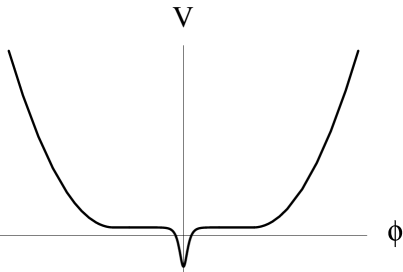
FIG. 7.: Scalar field potential in the cyclic scenario incorporating a stage of chaotic inflation. Inflationary perturbations are generated and the large-scale structure of the universe is produced both at $\phi<0$ and at $\phi>0$.

Thus we see that it is possible to propose a scenario describing an oscillating inflationary universe without making any assumptions about the behavior of non-inflationary perturbations near the singularity [52]. Another important advantage of this scenario is that inflationary cycles may begin in a universe with initial size as small as $O(1)$ in units of the Planck length, just as in the standard chaotic scenario [13].

Even though this scenario is free of many problems that plagued the old cyclic scenario [33], it still remains complicated and speculative. The main problem of this model is that one still must assume that somehow the universe can go through the singularity. However, now this assumption is no longer required for the success of the scenario since the large scale structure of the observable part of the universe in this scenario does not depend on processes near the singularity. This allows us to remove the remaining epicycles of this model.

FIG. 8.: The scalar field potential that appears after the step-by-step simplification of the cyclic scenario. It coincides with the simplest version of chaotic inflation scenario, Fig. 1.

Indeed, the main source of all the problems in this model is the existence of the minimum of the effective potential with $V(\phi)<0$. Once one cuts this minimum off, the potential becomes extremely simple, see Fig. 8, and all problems mentioned above disappear. In particular, one may use the simplest harmonic oscillator potential ${m^{2}\over 2}\phi^{2}+V_{0}$ with $V_{0}\sim 10^{-120}$ considered in the beginning of our paper. This theory describes an eternally self-reproducing chaotic inflationary universe, as well as the late stage of accelerated expansion (inflation) of the universe driven by the vacuum energy $V_{0}>0$.

XI Conclusions

In this paper I have briefly reviewed the basic principles of inflationary cosmology. During the last 20 years ago this theory has changed considerably and gradually become the standard framework for the investigation of the early universe. Recent observational data has brought us additional reasons to believe that we might be on the right track. It is quite encouraging that so far the simplest versions of inflationary cosmology seem to be in good agreement with observations. Still there are many things to do. We do not know which version of inflationary theory is the best. We do not even know whether the inflaton field is a scalar field, as in old, new and chaotic inflation, or something related to the curvature scalar, as in the Starobinsky model, or something else entirely like the logarithm of the radius of compactification or a distance between branes. It is possible to have several different stages of inflation; one could solve the homogeneity and isotropy problems while another could produce density perturbations. This latter stage may look like exponential expansion in all directions, or it may be viewed as exponential expansion on some particular hypersurface in a higher dimensional space.

Thus, there exist many different versions of inflationary cosmology, and many new ones will certainly appear with every new development in the theory of fundamental interactions. But one may wonder whether these new developments will eventually allow us to find a consistent non-inflationary cosmological theory? While we cannot give a general answer to this question, we hope that our investigation of the ekpyrotic/cyclic scenario demonstrates how difficult it is to construct a consistent cosmological theory without using inflation.

The original version of the ekpyrotic scenario [32] contained many incorrect and unproven statements [34, 35]. In particular, instead of expansion of the colliding branes described in [32], one has contraction to a singularity [35, 36]. Despite the optimistic statements of the authors of [32], the singularity problem in this scenario remains unsolved. The theory of density perturbations in this scenario is controversial; most authors believe that the mechanism of generation of density perturbations proposed in [32, 36] does not lead to adiabatic perturbations with a flat spectrum [38, 39, 40, 41]. Most importantly, this scenario offers no solution to major cosmological problems such as the homogeneity, flatness and entropy problems. In fact, the homogeneity problem in this scenario is even much more complicated than in the usual non-inflationary big bang theory [34].

As for the cyclic scenario [33], its authors recently issued a paper advertising this scenario in the popular press [72] and another one aimed at astrophysicists [73]. These new papers, which were supposed to give a summary of the state of the cyclic universe theory, omitted any mention of the criticisms of the ekpyrotic/cyclic scenario contained in [52] and in [34, 35, 38, 39, 40, 41, 51]. It was claimed in [73] that the cyclic scenario “is able to reproduce all of the successful predictions of the consensus model  (i.e. of inflationary cosmology -A.L.) with the same exquisite detail.” They continued by saying that “All of the differences between the two paradigms harken back to the disparate assumptions about whether there is a “beginning” or not.” Then they said that “if the big bang were not a beginning, but, rather, a transition from a pre-existing contracting phase, then the inflationary mechanism would fail.”

I cannot agree with these statements, for the reasons explained in Ref. [52] and in this paper. First of all, the cyclic scenario uses an infinite number of stages of inflation to solve the homogeneity problem, and therefore it is not an alternative to inflation. These stages of inflation are possible only if the universe is always huge. Thus, the flatness and entropy problems remain unsolved. This scenario is plagued by the singularity problem, and the situation with density perturbations is as obscure as in the ekpyrotic scenario. Finally, as was shown in [52], the simplest version of this scenario does not work in the way anticipated in [33] because of effects related to particle production. Just as in the ekpyrotic scenario [32], where the universe collapses instead of expanding [35], in the cyclic model of Ref. [33] the universe collapses instead of inflating [52].

In this paper, following [52], I described several ways to modify the cyclic model of Ref. [33] in order to avoid this problem. The simplest way is to make the potential positive both at $\phi\gg 0$ and at $\phi\ll 0$. This doubles the number of inflationary cycles but still leaves the scenario vulnerable with respect to the unknown physics at the singularity and to the problem of density perturbations.

One can resolve these problems by adding a stage of chaotic inflation after the singularity [52]. Indeed, contrary to the statement of Ref. [73], there is no reason to believe that the existence of a stage of contraction prior to the singularity should disallow inflation after the singularity. One should not represent inflation and the existence of the universe prior to the singularity as two incompatible possibilities.

The addition of an inflationary stage after the singularity allows one to use the standard inflationary mechanism of generation of density perturbations and makes all observational consequences of the theory indistinguishable from those in the usual chaotic inflation. However, in this scenario one still needs to assume that the universe can pass through the singularity, and one should use a non-standard mechanism of reheating after inflation.

But once we agree that one needs inflation in one way or another to solve the major cosmological problems, then why should one suffer with such complicated versions of inflationary theory? All of the problems discussed above completely disappear if one removes the minimum of the potential with $V(\phi)<0$. This final simplification reduces the theory to the standard chaotic inflation scenario describing an eternally self-reproducing inflationary universe, as well as the late stage of accelerated expansion of the universe.

This paper is dedicated to Stephen Hawking celebrating his 60th birthday, and therefore I would like to finish it on a positive note. So here it is:

The ekpyrotic/cyclic scenario is the best alternative to inflation that I am aware of.

I really mean it. I think that we should be very grateful to its authors. Indeed, if a model speculating about an infinite number of inflationary stages separated by an infinite number of singularities is the best alternative to inflation invented during the last 20 years, this means that inflationary theory is in a very good shape.

Note Added: After I wrote this paper, a new alternative to inflation was proposed by Hollands and Wald [74]. The authors admit that their new proposal does not solve any of the major cosmological problems addressed by inflation. However, they proposed a new hypothetical mechanism of generation of density perturbations with flat spectrum. We will discuss details of their proposal in a separate publication [75]. For the purposes of this paper it is sufficient to say that according to this new proposal the perturbations on the scale of the present horizon were generated at density $10^{96}$ times greater than the Planck density. This shows again how difficult it is to construct a consistent cosmological theory without using inflation.

REFERENCES

- [1] A. D. Linde, “A New Inflationary Universe Scenario: A Possible Solution Of The Horizon, Flatness, Homogeneity, Isotropy And Primordial Monopole Problems,” Phys. Lett. B 108, 389 (1982).
- [2] S. W. Hawking, I. G. Moss and J. M. Stewart, “Bubble Collisions In The Very Early Universe,” Phys. Rev. D 26, 2681 (1982).
- [3] A. H. Guth, “The Inflationary Universe: A Possible Solution To The Horizon And Flatness Problems,” Phys. Rev. D 23, 347 (1981).
- [4] A. H. Guth and E. J. Weinberg, “Could The Universe Have Recovered From A Slow First Order Phase Transition?,” Nucl. Phys. B 212, 321 (1983).
- [5] S. W. Hawking and I. G. Moss, “Supercooled Phase Transitions In The Very Early Universe,” Phys. Lett. B 110, 35 (1982).
- [6] A. Albrecht and P. J. Steinhardt, “Cosmology For Grand Unified Theories With Radiatively Induced Symmetry Breaking,” Phys. Rev. Lett. 48, 1220 (1982).
- [7] A. Vilenkin and L. H. Ford, “Gravitational Effects Upon Cosmological Phase Transitions,” Phys. Rev. D 26, 1231 (1982).
- [8] A. D. Linde, “Scalar Field Fluctuations In Expanding Universe And The New Inflationary Universe Scenario,” Phys. Lett. B 116, 335 (1982).
- [9] V. F. Mukhanov and G. V. Chibisov, “Quantum Fluctuation And ‘Nonsingular’ Universe,” JETP Lett. 33, 532 (1981) [Pisma Zh. Eksp. Teor. Fiz. 33, 549 (1981)].
- [10] S. W. Hawking, “The Development Of Irregularities In A Single Bubble Inflationary Universe,” Phys. Lett. B 115, 295 (1982); A. A. Starobinsky, “Dynamics Of Phase Transition In The New Inflationary Universe Scenario And Generation Of Perturbations,” Phys. Lett. B 117, 175 (1982); A. H. Guth and S. Y. Pi, “Fluctuations In The New Inflationary Universe,” Phys. Rev. Lett. 49, 1110 (1982); J. M. Bardeen, P. J. Steinhardt and M. S. Turner, “Spontaneous Creation Of Almost Scale - Free Density Perturbations In An Inflationary Universe,” Phys. Rev. D 28, 679 (1983).
- [11] V. F. Mukhanov, “Gravitational Instability Of The Universe Filled With A Scalar Field,” JETP Lett. 41, 493 (1985) [Pisma Zh. Eksp. Teor. Fiz. 41, 402 (1985)]; V. F. Mukhanov, H. A. Feldman and R. H. Brandenberger, “Theory Of Cosmological Perturbations,” Phys. Rept. 215, 203 (1992).
- [12] D. A. Kirzhnits, “Weinberg Model In The Hot Universe,” JETP Lett. 15, 529 (1972) [Pisma Zh. Eksp. Teor. Fiz. 15, 745 (1972)]; D. A. Kirzhnits and A. D. Linde, “Macroscopic Consequences Of The Weinberg Model,” Phys. Lett. B 42, 471 (1972); S. Weinberg, “Gauge And Global Symmetries At High Temperature,” Phys. Rev. D 9, 3357 (1974); L. Dolan and R. Jackiw, “Gauge Invariant Signal For Gauge Symmetry Breaking,” Phys. Rev. D 9, 2904 (1974); D. A. Kirzhnits and A. D. Linde, “A Relativistic Phase Transition,” Sov. Phys. JETP 40, 628 (1975) [Zh. Eksp. Teor. Fiz. 67, 1263 (1974)]; D. A. Kirzhnits and A. D. Linde, “Symmetry Behavior In Gauge Theories,” Annals Phys. 101, 195 (1976).
- [13] A. D. Linde, “Chaotic Inflation,” Phys. Lett. B 129, 177 (1983).
- [14] A.D. Linde, Particle Physics and Inflationary Cosmology (Harwood, Chur, Switzerland, 1990).
- [15] A. A. Starobinsky, “Spectrum Of Relict Gravitational Radiation And The Early State Of The Universe,” JETP Lett. 30, 682 (1979) [Pisma Zh. Eksp. Teor. Fiz. 30, 719 (1979)]; A. A. Starobinsky, “A New Type Of Isotropic Cosmological Models Without Singularity,” Phys. Lett. B 91, 99 (1980).
- [16] A. D. Dolgov and A. D. Linde, “Baryon Asymmetry In Inflationary Universe,” Phys. Lett. B 116, 329 (1982).
- [17] A. D. Dolgov and A. D. Linde, “Baryon Asymmetry In Inflationary Universe,” Phys. Lett. B 116, 329 (1982); L. F. Abbott, E. Farhi and M. B. Wise, “Particle Production In The New Inflationary Cosmology,” Phys. Lett. B 117, 29 (1982).
- [18] L. Kofman, A. D. Linde and A. A. Starobinsky, “Reheating after inflation,” Phys. Rev. Lett. 73, 3195 (1994) [arXiv:hep-th/9405187]; L. Kofman, A. D. Linde and A. A. Starobinsky, “Towards the theory of reheating after inflation,” Phys. Rev. D 56, 3258 (1997) [arXiv:hep-ph/9704452].
- [19] G. Felder, J. Garcia-Bellido, P. B. Greene, L. Kofman, A. Linde and I. Tkachev, “Dynamics of symmetry breaking and tachyonic preheating,” Phys. Rev. Lett. 87, 011601 (2001), hep-ph/0012142; G. Felder, L. Kofman and A. Linde, “Tachyonic Instability and Dynamics of Spontaneous Symmetry Breaking,” hep-th/0106179.
- [20] B. A. Ovrut and P. J. Steinhardt, “Supersymmetry And Inflation: A New Approach,” Phys. Lett. B 133, 161 (1983); B. A. Ovrut and P. J. Steinhardt, “Inflationary Cosmology And The Mass Hierarchy In Locally Supersymmetric Theories,” Phys. Rev. Lett. 53, 732 (1984); B. A. Ovrut and P. J. Steinhardt, “Locally Supersymmetric Cosmology And The Gauge Hierarchy,” Phys. Rev. D 30, 2061 (1984); B. A. Ovrut and P. J. Steinhardt, “Supersymmetric Inflation, Baryon Asymmetry And The Gravitino Problem,” Phys. Lett. B 147, 263 (1984).
- [21] A. D. Linde, “Eternally Existing Selfreproducing Chaotic Inflationary Universe,” Phys. Lett. B 175, 395 (1986).
- [22] A. D. Linde, “Axions in inflationary cosmology,” Phys. Lett. B 259, 38 (1991); A. D. Linde, “Hybrid inflation,” Phys. Rev. D 49, 748 (1994) [astro-ph/9307002].
- [23] E. J. Copeland, A. R. Liddle, D. H. Lyth, E. D. Stewart and D. Wands, “False vacuum inflation with Einstein gravity,” Phys. Rev. D 49, 6410 (1994) [astro-ph/9401011]; G. R. Dvali, Q. Shafi and R. Schaefer, “Large scale structure and supersymmetric inflation without fine tuning,” Phys. Rev. Lett. 73, 1886 (1994) [hep-ph/9406319]; E. D. Stewart, “Inflation, supergravity and superstrings,” Phys. Rev. D 51, 6847 (1995) [hep-ph/9405389].
- [24] P. Binetruy and G. Dvali, “D-term inflation,” Phys. Lett. B 388, 241 (1996) [hep-ph/9606342]; E. Halyo, “Hybrid inflation from supergravity D-terms,” Phys. Lett. B 387, 43 (1996) [hep-ph/9606423].
- [25] D. H. Lyth and A. Riotto, “Particle physics models of inflation and the cosmological density perturbation,” Phys. Rept. 314, 1 (1999) [hep-ph/9807278].
- [26] R. Kallosh, “N = 2 supersymmetry and de Sitter space,” arXiv:hep-th/0109168; C. Herdeiro, S. Hirano and R. Kallosh, “String theory and hybrid inflation/acceleration,” JHEP 0112 (2001) 027 [arXiv:hep-th/0110271]; K. Dasgupta, C. Herdeiro, S. Hirano and R. Kallosh, “D3/D7 inflationary model and M-theory,” arXiv:hep-th/0203019.
- [27] P. J. Steinhardt, “Natural Inflation,” UPR-0198T Invited talk given at Nuffield Workshop on the Very Early Universe, Cambridge, England, Jun 21 - Jul 9, 1982; A. D. Linde, “Nonsingular Regenerating Inflationary Universe,” Cambridge Univ. preprint Print-82-0554, (1982); A. Vilenkin, “The Birth Of Inflationary Universes,” Phys. Rev. D 27, 2848 (1983).
- [28] A. D. Linde, D. A. Linde and A. Mezhlumian, “From the Big Bang theory to the theory of a stationary universe,” Phys. Rev. D 49, 1783 (1994) [arXiv:gr-qc/9306035].
- [29] A. Borde, A. H. Guth and A. Vilenkin, “Inflation is not past-eternal,” arXiv:gr-qc/0110012.
- [30] J. L. Sievers, J. R. Bond, J. K. Cartwright, C. R. Contaldi, B. S. Mason, S. T. Myers, S. Padin, T. J. Pearson, U.-L. Pen, D. Pogosyan, S. Prunet, A. C. S. Readhead, M. C. Shepherd, P. S. Udomprasert, L. Bronfman, W. L. Holzapfel, J. May (U. de Chile), “Cosmological Parameters from Cosmic Background Imager Observations and Comparisons with BOOMERANG, DASI, and MAXIMA,” astro-ph/0205387.
- [31] D. Spergel and N. Turok, “Textures and cosmic structure,” Scientific American 266, 52 (1992).
- [32] J. Khoury, B. A. Ovrut, P. J. Steinhardt and N. Turok, “The ekpyrotic universe: Colliding branes and the origin of the hot big bang,” Phys. Rev. D 64, 123522 (2001) [arXiv:hep-th/0103239].
- [33] P. J. Steinhardt and N. Turok, “A cyclic model of the universe,” arXiv:hep-th/0111030; P. J. Steinhardt and N. Turok, “Cosmic evolution in a cyclic universe,” arXiv:hep-th/0111098; P. J. Steinhardt and N. Turok, “Is vacuum decay significant in ekpyrotic and cyclic models?,” arXiv:astro-ph/0112537;
- [34] R. Kallosh, L. Kofman and A. D. Linde, “Pyrotechnic universe,” Phys. Rev. D 64, 123523 (2001) [arXiv:hep-th/0104073].
- [35] R. Kallosh, L. Kofman, A. D. Linde and A. A. Tseytlin, “BPS branes in cosmology,” Phys. Rev. D 64, 123524 (2001) [arXiv:hep-th/0106241].
- [36] J. Khoury, B. A. Ovrut, N. Seiberg, P. J. Steinhardt and N. Turok, “From big crunch to big bang,” Phys. Rev. D 65, 086007 (2002) [arXiv:hep-th/0108187].
- [37] J. Khoury, B. A. Ovrut, P. J. Steinhardt and N. Turok, “Density perturbations in the ekpyrotic scenario,” arXiv:hep-th/0109050.
- [38] D. H. Lyth, “The primordial curvature perturbation in the ekpyrotic universe,” Phys. Lett. B 524, 1 (2002) [arXiv:hep-ph/0106153]; D. H. Lyth, “The failure of cosmological perturbation theory in the new ekpyrotic scenario,” Phys. Lett. B 526, 173 (2002) [arXiv:hep-ph/0110007].
- [39] R. Brandenberger and F. Finelli, “On the spectrum of fluctuations in an effective field theory of the ekpyrotic universe,” JHEP 0111, 056 (2001) [arXiv:hep-th/0109004]; F. Finelli and R. Brandenberger, “On the generation of a scale-invariant spectrum of adiabatic fluctuations in cosmological models with a contracting phase,” arXiv:hep-th/0112249.
- [40] J. c. Hwang, “Cosmological structure problem in the ekpyrotic scenario,” Phys. Rev. D 65, 063514 (2002) [arXiv:astro-ph/0109045]; J. c. Hwang and H. Noh, “Non-singular big-bounces and evolution of linear fluctuations,” arXiv:astro-ph/0112079; J. Hwang and H. Noh, “Identification of perturbation modes and controversies in ekpyrotic perturbations,” arXiv:hep-th/0203193.
- [41] J. Martin, P. Peter, N. Pinto Neto and D. J. Schwarz, “Passing through the bounce in the ekpyrotic models,” arXiv:hep-th/0112128; J. Martin, P. Peter, N. Pinto-Neto and D. J. Schwarz, “Comment on ’Density perturbations in the ekpyrotic scenario’,” arXiv:hep-th/0204222; P. Peter, J. Martin, N. Pinto-Neto and D. J. Schwarz, “Perturbations in the ekpyrotic scenarios,” arXiv:hep-th/0204227.
- [42] R. Durrer and F. Vernizzi, “Adiabatic perturbations in pre big bang models: Matching conditions and scale invariance,” arXiv:hep-ph/0203275.
- [43] P. Hor̆ava and E. Witten, Nucl. Phys. B475 (1996) 94 [hep-th/9603142]; E. Witten, Nucl. Phys. B 471, 135 (1996) [hep-th/9602070]; P. Hor̆ava, Phys. Rev. D 54, 7561 (1996) [hep-th/9608019]; T. Banks and M. Dine, Nucl. Phys. B 479, 173 (1996) [hep-th/9605136]; I. Antoniadis and M. Quiros, Phys. Lett. B 392, 61 (1997) [hep-th/9609209]; H. P. Nilles, M. Olechowski and M. Yamaguchi, Phys. Lett. B 415, 24 (1997) [hep-th/9707143]; H. P. Nilles, M. Olechowski and M. Yamaguchi,Nucl. Phys. B 530 (1998) 43 [hep-th/9801030]; H. P. Nilles, hep-ph/0004064.
- [44] K. Benakli, “Scales and cosmological applications of M-theory,” Phys. Lett. B 447, 51 (1999) [hep-th/9805181]; Z. Lalak, S. Pokorski and S. Thomas, “Beyond the standard embedding in M-theory on ,” Nucl. Phys. B 549, 63 (1999) [hep-ph/9807503].
- [45] R. Y. Donagi, J. Khoury, B. A. Ovrut, P. J. Steinhardt and N. Turok, “Visible branes with negative tension in heterotic M-theory,” JHEP 0111, 041 (2001) [arXiv:hep-th/0105199].
- [46] G. W. Moore, G. Peradze and N. Saulina, “Instabilities in heterotic M-theory induced by open membrane instantons,” Nucl. Phys. B 607, 117 (2001) [arXiv:hep-th/0012104].
- [47] A. Lukas, B. A. Ovrut and D. Waldram, Nucl. Phys. B 532, 43 (1998) [hep-th/9710208]; Phys. Rev. D 57, 7529 (1998) [hep-th/9711197]; A. Lukas, B. A. Ovrut, K. S. Stelle and D. Waldram, Phys. Rev. D 59, 086001 (1999) [hep-th/9803235]; A. Lukas, B. A. Ovrut, K. S. Stelle and D. Waldram, Nucl. Phys. B552, 246 (1999) [hep-th/9806051].
- [48] H. Liu, G. Moore and N. Seiberg, “Strings in a time-dependent orbifold,” arXiv:hep-th/0204168.
- [49] N. A. Nekrasov, “Milne universe, tachyons, and quantum group,” arXiv:hep-th/0203112.
- [50] N. Seiberg, “String Theory on a Time Dependent Orbifold,” a seminar at the UCSC, 29 April 2002; J. Polchinski, privite communication.
- [51] S. Rasanen, “On ekpyrotic brane collisions,” Nucl. Phys. B 626, 183 (2002) [arXiv:hep-th/0111279].
- [52] G. Felder, A. Frolov, L. Kofman and A. Linde, “Cosmology with negative potentials,” arXiv:hep-th/0202017; to be published in Phys. Rev. D
- [53] T. Banks and M. Dine, “Phenomenology of strongly coupled heterotic string theory,” arXiv:hep-th/9609046.
- [54] A. D. Linde, “Quantum Creation Of The Inflationary Universe,” Lett. Nuovo Cim. 39, 401 (1984); A. Vilenkin, “Quantum Creation Of Universes,” Phys. Rev. D 30, 509 (1984).
- [55] R. Kallosh, L. Kofman, A. D. Linde and A. Van Proeyen, “Superconformal symmetry, supergravity and cosmology,” Class. Quant. Grav. 17, 4269 (2000) [arXiv:hep-th/0006179].
- [56] L. H. Ford, “Gravitational Particle Creation And Inflation,” Phys. Rev. D 35, 2955 (1987).
- [57] Ya. B. Zel’dovich and A. A. Starobinsky, “Particle Production And Vacuum Polarization In An Anisotropic Gravitational Field,” Zh. Exp. Theor. Fiz. 61, 2161 (1971) [Sov. Phys. JETP 34, 1159 (1972)]; L. P. Grishchuk, “The Amplification Of Gravitational Waves And Creation Of Gravitons In The Isotropic Universes,” Lett. Nuovo Cim. 12, 60 (1975); Sov. Phys. JETP 40, 409 (1975); S. G. Mamaev, V. M. Mostepanenko and A. A. Starobinsky, “Particle Creation From Vacuum Near An Homogeneous Isotropic Singularity,” Zh. Eksp. Teor. Fiz. 70, 1577 (1976) [Sov. Phys. JETP 43, 823 (1976)]; A. A. Grib, S. G. Mamaev and V. M. Mostepanenko, “Particle Creation From Vacuum In Homogeneous Isotropic Models Of The Universe,” Gen. Rel. Grav. 7, 535 (1976); A.A. Grib, S.G. Mamaev, and V. M. Mostepanenko, Vacuum Quantum Effects in Strong Fields (Energoatonizdat, Moscow, 1988).
- [58] A. V. Toporensky, “The degree of generality of inflation in FRW models with massive scalar field and hydrodynamical matter,” Grav. Cosmol. 5, 40 (1999) [arXiv:gr-qc/9901083].
- [59] A. J. Tolley and N. Turok, “Quantum fields in a big crunch/big bang spacetime,” arXiv:hep-th/0204091.
- [60] R.C. Tolman, Phys. Rev. 38, 1758 (1931); G. Lemaître, Ann. Soc. Sci. Bruxelles A 53, 51 (1933), translated in Gen Rel. Grav. 29, 935 (1997); R. Dicke, and P.J.E. Peebles, in: General relativity, eds., S.W. Hawking, and W. Israel, (Cambridge Univ. Press, Cambridge, 1979), 504p.
- [61] R.C. Tolman, Relativity, thermodynamics and cosmology, (Oxford Univ. Press, London, 1934).
- [62] P.J.E. Peebles, Principles of physical cosmology (Princeton Univ. Press, Princeton, 1993).
- [63] M. A. Markov, “Problems Of A Perpetually Oscillating Universe,” Annals Phys. 155, 333 (1984).
- [64] A. D. Linde, “The Inflationary Universe,” Rept. Prog. Phys. 47, 925 (1984), Appendix 1.
- [65] R. H. Brandenberger and C. Vafa, “Superstrings In The Early Universe,” Nucl. Phys. B 316, 391 (1989).
- [66] R. H. Brandenberger, V. Mukhanov and A. Sornborger, “A Cosmological theory without singularities,” Phys. Rev. D 48, 1629 (1993) [arXiv:gr-qc/9303001].
- [67] G. Veneziano, “Scale factor duality for classical and quantum strings,” Phys. Lett. B 265, 287 (1991); M. Gasperini and G. Veneziano, “Pre - big bang in string cosmology,” Astropart. Phys. 1, 317 (1993) [arXiv:hep-th/9211021].
- [68] M. S. Turner and E. J. Weinberg, “Pre-big-bang inflation requires fine tuning,” Phys. Rev. D 56, 4604 (1997) [arXiv:hep-th/9705035]; N. Kaloper, A. D. Linde and R. Bousso, “Pre-big-bang requires the universe to be exponentially large from the very beginning,” Phys. Rev. D 59, 043508 (1999) [arXiv:hep-th/9801073]; A. Buonanno and T. Damour, “The fate of classical tensor inhomogeneities in pre-big-bang string cosmology,” Phys. Rev. D 64, 043501 (2001) [arXiv:gr-qc/0102102].
- [69] B.Spokoiny, “Deflationary universe scenario,” Phys. Lett. B 315, 40 (1993) [arXiv:gr-qc/9306008]; MM. Joyce, “On the expansion rate of the universe at the electroweak scale,” Phys. Rev. D 55, 1875 (1997) [arXiv:hep-ph/9606223]; M. Joyce and T. Prokopec, “Turning around the sphaleron bound: Electroweak baryogenesis in an alternative post-inflationary cosmology,” Phys. Rev. D 57, 6022 (1998) [arXiv:hep-ph/9709320]; P. J. Peebles and A. Vilenkin, “Quintessential inflation,” Phys. Rev. D 59, 063505 (1999) [arXiv:astro-ph/9810509]; D. J. Chung, E. W. Kolb and A. Riotto, “Superheavy dark matter,” Phys. Rev. D 59, 023501 (1999) [arXiv:hep-ph/9802238]; V. Kuzmin and I. Tkachev, “Matter creation via vacuum fluctuations in the early universe and observed ultra-high energy cosmic ray events,” Phys. Rev. D 59, 123006 (1999) [arXiv:hep-ph/9809547]; G. N. Felder, L. Kofman and A. D. Linde, “Gravitational particle production and the moduli problem,” JHEP 0002, 027 (2000) [arXiv:hep-ph/9909508]; G. F. Giudice, A. Riotto and I. I. Tkachev, “The cosmological moduli problem and preheating,” JHEP 0106, 020 (2001) [arXiv:hep-ph/0103248].
- [70] G. N. Felder, L. Kofman and A. D. Linde, “Instant preheating,” Phys. Rev. D 59, 123523 (1999) [arXiv:hep-ph/9812289].
- [71] G. N. Felder, L. Kofman and A. D. Linde, “Inflation and preheating in NO models,” Phys. Rev. D 60, 103505 (1999) [arXiv:hep-ph/9903350].
- [72] P. J. Steinhardt and N. Turok, “A Cyclic Model of the Universe,” Science, Published online April 25, 2002; 10.1126/science.1070462 (Science Express Research Articles).
- [73] P. J. Steinhardt and N. Turok, “The cyclic universe: An informal introduction,” arXiv:astro-ph/0204479.
- [74] S. Hollands and R. M. Wald, “An alternative to inflation,” arXiv:gr-qc/0205058.
- [75] L. Kofman, A. Linde and V. Mukhanov, in preparation.