Riemannian Gauge Theory and Charge Quantization

Abstract:

In a traditional gauge theory, the matter fields $\phi^{a}$ and the gauge fields $A^{c}_{\mu}$ are fundamental objects of the theory. The traditional gauge field is similar to the connection coefficient in the Riemannian geometry covariant derivative, and the field-strength tensor is similar to the curvature tensor. In contrast, the connection in Riemannian geometry is derived from the metric or an embedding space. Guided by the physical principal of increasing symmetry among the four forces, we propose a different construction. Instead of defining the transformation properties of a fundamental gauge field, we derive the gauge theory from an embedding of a gauge fiber $F={\bf R}^{n}$ or $F={\bf C}^{n}$ into a trivial, embedding vector bundle ${\tilde{F}}={\bf R}^{N}$ or ${\tilde{F}}={\bf C}^{N}$ where $N>n$. Our new action is symmetric between the gauge theory and the Riemannian geometry. By expressing gauge-covariant fields in terms of the orthonormal gauge basis vectors, we recover a traditional, $SO(n)$ or $U(n)$ gauge theory. In contrast, the new theory has all matter fields on a particular fiber couple with the same coupling constant. Even the matter fields on a ${\bf C}^{1}$ fiber, which have a $U(1)$ symmetry group, couple with the same charge of $\pm q$. The physical origin of this unique coupling constant is a generalization of the general relativity equivalence principle. Because our action is independent of the choice of basis, its natural invariance group is $GL(n,{\bf R})$ or $GL(n,{\bf C})$. Last, the new action also requires a small correction to the general-relativity action proportional to the square of the curvature tensor.

1 Traditional Gauge Theory

In a traditional gauge theory [1, p. 7], the matter fields $\phi^{a}$ and the gauge fields $A^{c}_{\mu}$ are fundamental objects of the theory with $(A_{\mu})^{a}_{\ b}(x)=(T^{c})^{a}_{\ b}A_{\mu}^{c}(x)$, where the $T^{c}$ are the generators of the gauge group $G$. The gauge theory is defined by the properties given to these fundamental fields. One defines a continuous local symmetry group $G$  and a transformation rule $\phi^{\prime a}(x)=g^{a}_{\ b}(x)\,\phi^{b}(x)$ for every multiplet $\phi^{a}(x)$ of matter fields, where $g(x)$ is some representation of $G$. One maintains the gauge invariance of the matter-field derivative by introducing a gauge field $A_{\mu}$ and a gauge-field transformation rule

$$(A^{\prime}_{\mu})^{a}_{\ b}=g^{a}_{\ c}\,(A_{\mu})^{c}_{\ d}\,{(g^{-1})}^{d}_{\ b}+(i/q)\,g^{a}_{\ c}\,\partial_{\mu}\,{(g^{-1})}^{c}_{\ b}$$ (1)

that cancels the extra term appearing in the derivative $\partial_{\mu}(g\,\phi)$. These properties are collected and clearly defined in terms of principal bundles [2]. In the action, one includes every Lorentz-invariant, gauge-invariant, renormalizable interaction.

The traditional gauge theory with a fundamental gauge field has many parallels with Riemannian geometry [3, 4, 5]. The covariant derivatives of a matter field $\phi^{a}$ appear together with the gauge fields, $D_{\mu}\phi^{a}=(\delta^{a}_{b}\partial_{\mu}-iq(A_{\mu})^{a}_{\ b})\phi^{b}$, in a structure that resembles the covariant derivatives of a vector $V^{\nu}$ in Riemannian geometry $\nabla_{\mu}V^{\nu}=(\delta^{\sigma}_{\mu}\partial_{\sigma}+\Gamma^{\mu}_{\nu\sigma})V^{\sigma}$. The field-strength tensor $F_{\mu\nu}$, which is constructed to maintain the gauge invariance of ${\rm Tr}(F_{\mu\nu}F^{\mu\nu})$, is the commutator of two covariant derivatives

$$-i\,{F_{\mu\nu}}^{a}_{\ b}\phi^{b}=([D_{\mu},D_{\nu}]\phi)^{a}$$ (2)

as is the curvature tensor of Riemannian geometry

$$-R^{\ \ \lambda}_{\mu\nu\ \sigma}V^{\sigma}=([\nabla_{\mu},\nabla_{\nu}]V)^{\lambda}.$$ (3)

Unlike a traditional gauge theory, the connection in Riemannian geometry is not fundamental and can be derived from a metric or an embedding. Thanks to a proof by John Nash [6], these two approaches are equivalent. For every Riemannian metric, one can always find an isometric embedding into a larger-dimensional flat space such that the pull-back gives the same Riemannian metric. These two equivalent ways to understand the connection each have advantages. The derivation of the connection from a fundamental metric never uses dimensions outside the embedded manifold. The derivation of the connection from an explicit embedding aids in the understanding or visualization of the geometry.

The parallels between gauge theory and Riemannian geometry lead to our first question: Does a $U(n)$ gauge theory have an analogous embedding from which one can derive the gauge field and can visualize the geometry? The answer is yes. In 1961, Narasimhan and Ramanan [7, 8] showed such an embedding. They showed a surjective map from an embedding of a ${\bf C}^{n}$-vector bundle into a trivial ${\bf C}^{N}$-vector bundle ($N>n$) onto a standard $U(n)$ gauge theory, and they proved that such an embedding exists for every $U(n)$ gauge field if $N\geq(2\,d+1)n^{3}$ where $d$ is the number of space-time dimensions. Since then, Atiyah [9]; Corrigan Fairlie, Templeton, and Goddard [10]; Dubois-Violette and Georgelin [11]; Cahill and Raghavan [12] all have used this map to represent traditional gauge theories, as have others more recently [13, 14]. Although not identical, this map from an embedding to a gauge field is similar to the corner variables of Bars [15, 16] and the degenerate subspace described by Wilczek and Zee [17]. In this paper, we study this gauge-field embedding applied to abelian gauge theories.

Previous work is discussed in sections 1 through 4. First, this section reviews traditional gauge theories. Next in section 2, we show how the traditional gauge theory leads to the charge quantization puzzle. Section 3 reviews how the metric and the connection are derived from an embedding. In comparison to section 3, we explain in section 4 the map from the embedding onto a traditional gauge theory. Nearly all previous work on embedded gauge theories focused on non-abelian gauge theories; therefore, they took the unique coupling constant as a given and they dealt with vector bundles of too large a dimension to easily visualize.

New material is covered in sections 5 through 8. In contrast to previous work, we focused our research on a very simple example: an $SO(2)$ gauge theory, which is equivalent to a $U(1)$ gauge theory. In section 5, we visualize this case as an ${\bf{R}}^{2}$-vector bundle embedded into a trivial ${\bf{R}}^{3}$-vector bundle. These simple $SO(2)$ examples forced us to face questions not addressed in previous work: questions of charge and coupling constants for different fields, and questions of basis vector normalization. We found that to make the $SO(2)$ examples self-consistent, we needed to define a new type of gauge theory that we call Riemannian gauge theory. In section 6, we introduce the Riemannian-gauge-theory action. Our new action is built on the physical principle that a natural description of nature should treat the four known forces with some degree of symmetry. In this action, the gauge covariant derivative is derived from an embedding and not defined by its transformation properties. In the total space, the action treats all four forces equivalently. Distinct forces arise after taking the projection that defines the various fiber bundles. With an appropriate gauge choice, our new action is nearly identical to the traditional-gauge-theory action. Section 7 emphasizes that the new action does not have the freedom to choose distinct coupling constants for different matter-fields and addresses the multiple $U(1)$ coupling constants in the standard model. In section 8, we observe that the action has a larger $GL(n,{\bf{C}})$ local symmetry where the gauge metric satisfies the metric compatibility condition. This result is in sharp contrast to a traditional gauge theory of a non-compact group. In the last section, we give our concluding remarks.

2 Charge Quantization History

Traditional gauge theories naturally quantize the charges of non-abelian gauge groups but not those of abelian groups.

In the abelian case, each field $\phi_{i}$ can be defined with a transformation law specific to its own coupling constant $q_{i}$. The abelian field-strength tensor (2) is a linear function of the coupling constant, $F(q_{1}+q_{2},A)=F(q_{1},A)+F(q_{2},A)$, and of the gauge fields, $F(q,A_{1}+A_{2})=F(q,A_{1})+F(q,A_{2})$. The field-strength term $\alpha\,F_{\mu\nu}F^{\mu\nu}$ in the action can be multiplied by any constant $\alpha$. Because of the field-strength tensor’s linearity and the arbitrariness of $\alpha$, the covariant derivative of any field $\phi_{i}$ can be used in eq.(2) to define $F_{\mu\nu}$. The field-strength tensor is strictly gauge invariant regardless of which coupling constant one chooses in the gauge-field transformation rule (1).

In contrast, a non-abelian gauge group only allows one coupling constant $q$ for all non-trivially transforming fields. The non-abelian field-strength tensor is not linear in the coupling constant, nor is it linear in the gauge field. If different fields had different coupling constants, then one would have to choose which coupling constant to use in the gauge-field transformation rule (1) of the gauge fields in the field-strength tensor. Also, one would need to transform the gauge fields in the field-strength tensor differently from the gauge fields in the covariant derivatives of the matter fields. This difference would violate gauge invariance. So all fields transforming under a non-abelian gauge group must have the same coupling constant.

The coupling constant is different from the charge. In the non-abelian case, one will have different charges for matter-field multiplets proportional to different eigenvectors of the group generators. Simple groups will have quantized charges. In contrast, an abelian group has a continuum of eigenvalues, and the matter fields may be proportional to any corresponding eigenvector. In the abelian case, no mathematical difference distinguishes fields coupling with different coupling constants from fields coupling with the same coupling constant but with different charges.

As far as we know, matter fields with an abelian gauge group have charges that are integral multiples of $q_{e}/3$ where $q_{e}$ is the free-space charge of the electron. The electric-charge quantization problem is the conflict between these quantized electric charges and the unconstrained continuum of allowable electric charges.

Several physicists have offered explanations for the quantization of electric charge. Dirac [18] in 1931 showed that if magnetic monopoles exist, they would quantize electric charge. Georgi and Glashow [19] and Pati and Salam [20] explained the charges of the fermions by associating the photon with a traceless generator of an $SU(n)$ unification group. Others [21, 22, 23, 24, 25, 26] have exploited anomaly cancellation.

3 Metric and Connection from an Embedding

In Riemannian geometry [2, 27, 28], the covariant derivative may be defined by properties of the connection and the metric, or in-terms of a hypothetical flat embedding space. In this section, we present the Riemannian geometry framework of these two methods.

First, we define the manifold with the tangent bundle. A projection $\pi:E\rightarrow M$ from a total space $E$ to a real, $d$-dimensional base manifold $M$ gives rise to a fiber bundle that is the collection of vector spaces $\pi^{-1}(x)={\bf R}^{d}$ for every space-time point $x\in M$. Because the fiber $\pi^{-1}(x)$ is a vector space, the fiber bundle is also a vector bundle.

The set of tangent vectors at a point $x$ is the set of vectors that are tangent to all possible smooth, differentiable curves that pass through $x$. The fiber $\pi^{-1}(x)$ becomes a tangent space at the point $p$ when one identifies directions and lengths on the fiber with directions and lengths on the base manifold. This identification maps the set of tangent vectors at $x$ onto the vector space $\pi^{-1}(x)$. Since the tangent fiber is a flat tangent plane, only one set of basis vectors $t_{\mu}(x)$ at a fixed origin $O\in\pi^{-1}(x)$ is needed to fully define coordinates on the tangent space.

A vector field ${V}$ is a tangent-space vector that varies smoothly with the point $p$ in $M$. In a particular basis ${t}$, the vector field is given by ${V}=V^{\mu}{t}_{\mu}$ where the Greek indices run through the dimensionality of the base manifold. The functions $V^{\mu}$ are real-valued coefficients (i.e., not vectors) of the basis vectors $t_{\mu}$. A common choice for ${t}_{\mu}$ is the coordinate tangent vectors, ${t}_{\mu}=\partial_{\mu}$.

In addition to basis vectors, we need dual basis vectors and an inner product. The dual basis vector ${{{t}}}^{\mu}$ is defined as the linear operator on the basis vectors that returns the Kronecker delta: ${{{t}}}^{\mu}({t}_{\nu})=\delta^{\mu}_{\nu}$. The dual basis vectors combine with the basis vectors to form a projection operator $P=t_{\mu}\,{{{t}}}^{\mu}$ which projects vectors onto the tangent space. For a vector $V$ in the tangent space, the projection operator gives simply, ${P}({V})={t}_{\mu}{{{t}}}^{\mu}(V^{\alpha}{t}_{\alpha})={t}_{\mu}V^{\alpha}\delta_{\alpha}^{\mu}={t}_{\mu}V^{\mu}={V}$. The inner product $\langle V,W\rangle$ measures the length or the point-wise overlap of two vector fields; the inner product of two tangent vectors is the metric, $g_{\mu\nu}=\langle t_{\mu},t_{\nu}\rangle$. In a particular basis, the inner product of two vectors is $\langle V,W\rangle=\langle V^{\mu}t_{\mu},W^{\nu}t_{\nu}\rangle=V^{\mu}W^{\nu}\langle t_{\mu},t_{\nu}\rangle=V^{\mu}W^{\nu}g_{\mu\nu}$.

Given our fiber bundle $\pi:E\rightarrow M$, the metric on the total space $E$ will be bundle-like [29, 30]. A bundle-like metric will satisfy two properties relevant to this paper. First, a bundle-like metric can be made block diagonal in fiber components and the base-manifold components [29]. Second, a bundle-like metric will have $\partial_{j}g_{\mu\nu}=0$ where $\partial_{j}$ denotes a derivative with respect to a coordinate that is tangent to the fiber at a base-manifold point and where $g_{\mu\nu}$ are the base-manifold components of the total space metric [30].

We will now show two methods to define the covariant derivative. The first defines properties of the connection and the metric, and the second is from a flat embedding space.

The covariant derivative $\nabla_{X}V$ can be defined as a map from two vector fields $X$ and $V$ to a new vector field. The map must be linear in $X$, linear in $V$, and must satisfy the product rule [27]. The covariant derivative of a vector field $V$ in the direction $X^{\sigma}{t}_{\sigma}$ is written as

$$\nabla_{X}(V)\equiv X^{\sigma}t_{\alpha}(\delta^{\alpha}_{\mu}\partial_{\sigma}+\Gamma^{\alpha}_{\sigma\mu})V^{\mu}$$ (4)

where the Christoffel symbols $\Gamma^{\alpha}_{\sigma\mu}$ define the connection. We further define the metric $g$ to satisfy $\nabla_{X}g\equiv 0$. These requirements lead to a unique connection $\Gamma^{\alpha}_{\sigma\nu}$ for a given metric $g$, $\Gamma^{\alpha}_{\sigma\nu}=\frac{1}{2}g^{\alpha\lambda}(\partial_{\sigma}g_{\lambda\nu}+\partial_{\nu}g_{\sigma\lambda}-\partial_{\lambda}g_{\sigma\nu})$.

Another way to introduce a covariant derivative is to embed the manifold $M$ in a Euclidean (or Lorentzian) space ${\tilde{M}}$ of higher dimension, $X:M\rightarrow{\tilde{M}}$. Vectors in ${\tilde{M}}$ are compared in the derivative by means of ordinary parallel transport in the embedding space. Using the embedding space, the covariant derivative of a vector field $V$ in the direction ${t}_{\sigma}$ is:

$$\nabla_{\sigma}(V) \equiv P(\partial_{\sigma}(V^{\alpha}t_{\alpha}))\equiv t_{\alpha}(\delta^{\alpha}_{\mu}\partial_{\sigma}+\Gamma^{\alpha}_{\sigma\mu})V^{\mu}$$ (5)

$$\nabla_{\sigma}(V) = P(t_{\alpha}\partial_{\sigma}V^{\alpha}+V^{\alpha}\partial_{\sigma}t_{\alpha})=t_{\alpha}\,\left(\delta_{\mu}^{\alpha}\partial_{\sigma}+{{{t}}}^{\alpha}(\partial_{\sigma}t_{\mu})\right)V^{\mu}.$$ (6)

The Christoffel symbols

$$\Gamma^{\alpha}_{\sigma\mu}\equiv{{{t}}}^{\alpha}(\partial_{\sigma}t_{\mu})$$ (7)

are the projection onto the tangent space of the derivative of the tangent vectors $t_{\mu}$ in the direction ${t}_{\sigma}$.

If one begins with the properties of the connection, Nash [6] proved that an isometric embedding $X$ is always possible with ${\tilde{M}}={\bf R}^{D}$ as long as $D\geq d(3d+11)/2$. The explicit tangent vectors are found by coordinate derivatives on the coordinates of the embedding function ${\tilde{t}}_{\mu}^{\ j}=\frac{\partial}{\partial x^{\mu}}X^{j}(x)$ yielding a $d\times D$-dimensional rectangular matrix. The metric on $M$ is given by the inner product of two basis vectors $\langle t_{\mu},t_{\nu}\rangle=g_{\mu\nu}=\delta_{ij}{\tilde{t}}_{\mu}^{i}{\tilde{t}}_{\nu}^{j}$. This explicit embedding aids understanding and visualization.

In Riemannian geometry, tangent-space basis vectors can completely describe the intrinsic properties of the manifold such as the connection, the metric, and the curvature tensors. They can also describe quantities that are not inherent to the manifold, such as the vector fields.

4 Gauge Field from an Embedding

In section 1, we reviewed traditional gauge theory where the gauge fields are fundamental fields in the theory. In this section, we review the way to derive the gauge fields from an embedding built on the work of Narasimhan and Ramanan [7, 8].

We begin with a vector bundle given by a projection $\pi_{F}:E_{F}\rightarrow M$ from a total space $E_{F}$ to a space-time base manifold $M$. The subscript $F$ denotes the projection that creates the fiber. The gauge vector bundle is the collection of vector spaces $\pi_{G}^{-1}(x)=F|_{x}$ for every point $x\in M$. The fundamental matter field determines the choice of the vector space $F|_{x}$. For example, if $\phi$ is a real, $n$-dimensional matter-field multiplet, then the fiber is $F|_{x}=\bf{R}^{n}$; and if $\phi$ is a complex, $n$-dimensional field, then the fiber is $F|_{x}=\bf{C}^{n}$. We shall refer to the vector space $F|_{x}$ as the fiber or the gauge fiber in what follows.

The geometry of the gauge vector bundle differs from the tangent bundle because directions or lengths on the fiber $F|_{x}$ are not identified with directions or lengths on the base manifold. Directions and lengths on the gauge fiber are identified with directions and lengths on the total space $E_{F}$; however, these coordinates disappear under the projection $\pi_{F}$. Like the tangent fiber, the gauge fiber is a flat plane, and so only one basis-vector set $e_{a}(x)$ at a fixed origin $O\in F|_{x}$ is needed to fully define its coordinates.

As in Riemannian geometry, a matter field $\phi(x)\in F_{p}$ varies smoothly with the point $x\in M$. In terms of a local basis $e_{a}(x)$ on $F|_{x}$, the matter field is given by $\phi(x)=\phi^{a}(x)e_{a}(x)$ where the Latin indices run through the dimensionality of the gauge fiber. The component $\phi^{a}(x)$ of the matter field $\phi(x)$ is a coefficient of a basis vector $e_{a}(x)$ and is not itself a vector. The complex conjugate of the component $\phi^{a}$ is denoted $\phi^{\bar{a}}\equiv{\overline{\phi^{a}}}$, similarly $e_{\bar{a}}\equiv{\overline{e_{a}}}$. The components $\phi^{\bar{a}}$ are the coefficients of the complex-conjugate basis vectors, as in ${\overline{\phi}}=\phi^{\bar{a}}e_{\bar{a}}$.

In addition to basis vectors, we need dual basis vectors and an inner product. Like the dual basis vectors of Riemannian geometry, the dual basis vector ${{{e}}}^{a}$ is defined as the linear operator on the basis vectors that returns the Kronecker delta: ${{{e}}}^{a}(e_{b})=\delta^{a}_{b}$. The dual basis vectors combine with the basis vectors to form a projection operator $P=e_{a}{{{e}}}^{a}$ which projects vectors onto the gauge fiber. For a matter field $\phi$ in the gauge fiber, the projection operator gives simply, $P(\phi)=e_{a}{{{e}}}^{a}(\phi^{c}e_{c})=e_{a}\phi^{c}\delta^{a}_{c}=e_{c}\phi^{c}=\phi$. A complex vector space also has dual vectors for the complex conjugate of the basis vectors ${{{e}}}^{\bar{a}}(e_{\bar{b}})=\delta^{\bar{a}}_{\bar{b}}$. By definition [2, p. 275], one has ${{{e}}}^{\bar{a}}(e_{b})=0$ and ${{{e}}}^{a}(e_{\bar{b}})=0$.

We use the notation $\langle\phi,\psi\rangle$ to denote the inner product of two matter vector fields, $\phi$ and $\psi$. In quantum mechanics, inner products are used to compute lengths and probability amplitudes. The inner product of the basis vectors of the fiber $F|_{x}$ is the gauge-fiber metric $g_{\bar{a}b}=\langle e_{a},e_{b}\rangle$, which is distinguished by its Latin indices from the metric $g_{\mu\nu}$ of the base manifold $M$. The inner product of two complex matter vectors is $\langle\phi,\psi\rangle=\langle\phi^{a}e_{a},\psi^{b}e_{b}\rangle={\phi^{\bar{a}}}\psi^{b}g_{\bar{a}b}$. This inner product uses a hermitian metric, ${\overline{g_{\bar{a}b}}}=g_{\bar{b}a}$, which by definition also satisfies $g_{\bar{a}\bar{b}}=g_{ab}=0$. The gauge-fiber metric is defined so that $g_{\bar{a}b}=g_{b\bar{a}}$ and ${\overline{g_{\bar{a}b}}}=g_{a\bar{b}}$. The quantity $g^{a\bar{b}}$ is the inverse of the fiber metric, $g^{a\bar{b}}g_{\bar{b}c}=\delta^{a}_{c}$. The fiber metric and its inverse can raise and lower indices:

$$\phi_{\bar{a}}=g_{\bar{a}b}\phi^{b}\qquad\phi^{\bar{a}}=g^{\bar{a}b}\phi_{b}.$$ (8)

Because $g^{ab}=0$, we cannot get $\phi^{a}$ by using $g^{ab}$ to raise an index. Instead we write $\phi^{a}=g^{a\bar{b}}\phi_{\bar{b}}$.

All previous research in gauge theories with an explicit embedding space assumed orthonormal basis vectors with a trivial gauge fiber metric. We have generalized the approach in the literature to make manifest the symmetry with Riemannian geometry.

Given our fiber bundle $\pi_{F}:E_{F}\rightarrow M$, the metric on the total space $E_{F}$ will be bundle-like [29, 30]. A bundle-like metric will satisfy two properties relevant to this paper. First, a bundle-like metric can be made block diagonal in fiber components and the base-manifold components [29]. Second, a bundle-like metric will have $\partial_{a}g_{\mu\nu}=0$ where $\partial_{a}$ denotes a derivative with respect to a coordinate that is tangent to the fiber of a base-manifold point and where $g_{\mu\nu}$ are the base-manifold components of the total space metric [30].

Like the covariant derivative in Riemannian geometry, the gauge-covariant derivative of a matter multiplet $\phi$ in the direction $t_{\sigma}$ is the projection onto the gauge fiber of the derivative of the matter multiplet $\phi$ in the direction $t_{\sigma}$:

$$D_{\sigma}(\phi)\equiv P(\partial_{\sigma}(e_{a}\phi^{a}))\equiv e_{a}\left(\delta^{a}_{b}\partial_{\sigma}-i(A_{\mu})^{a}_{\ b}\right)\phi^{b}$$ (9)

$$D_{\sigma}(\phi)=P(e_{a}\partial_{\sigma}\phi^{a}+\phi^{a}\partial_{\sigma}e_{a})=e_{a}\left(\delta^{a}_{b}\partial_{\sigma}+{{{e}}}^{a}(\partial_{\sigma}e_{b})\right)\phi^{b},$$ (10)

where the gauge field is

$$(A_{\mu})^{a}_{\ b}=i{{{e}}}^{a}(\partial_{\mu}e_{b}).$$ (11)

We compare basis vectors at different points of the manifold by embedding the gauge fiber $F$ in a trivial, real or complex Euclidean vector bundle $M\times{\tilde{F}}$ with a fiber ${\tilde{F}}$ of higher dimension: $F\rightarrow{\tilde{F}}$. In the spirit of Nash’s embedding theorem [6], Narasimhan and Ramanan [7, 8] showed that for any $U(n)$ or $SO(n)$ gauge field, one can embed the gauge fiber $F$ in a trivial embedding fiber ${\tilde{F}}$ of dimension $N\geq(2\,d+1)n^{3}$. The basis vectors of the fiber $F\subset{\tilde{F}}$ now are the orthonormal vectors ${\tilde{e}}^{\ j}_{a}$, where the index $j$ runs from 1 to $N$. The $n$ basis vectors $e_{a}$ of $F$ are each $N$-vectors ${\tilde{e}}_{a}^{\ j}$ in the trivial fiber and span an $n$-dimensional subspace of ${\tilde{F}}$. The embedding space may now be used to express the projection operator

$$P^{j}_{\ k}={\tilde{e}}_{a}^{\ j}\,{{{{\tilde{e}}}}}^{a}_{\ k}$$ (12)

and the metric

$$g_{\bar{a}b}={\overline{{\tilde{e}}^{\ k}_{a}}}\,{\tilde{e}}^{\ j}_{b}\,\delta_{\bar{k}j}={\tilde{e}}_{\bar{a}j}\,{\tilde{e}}^{\ j}_{b}=\sum_{j=1}^{N}\,{\overline{{\tilde{e}}_{aj}}}\,{\tilde{e}}_{bj},$$ (13)

in which the bar denotes ordinary complex conjugation. The quantity $\delta_{\bar{j}k}$ may be interpreted as a hermitian metric on a complex Euclidean embedding fiber.

Narasimhan and Ramanan based their embedding theorem on orthonormal basis vectors $\langle e_{a},e_{b}\rangle=\delta_{\bar{j}k}\,{\overline{{\tilde{e}}_{a}^{\ j}}}\,{\tilde{e}}_{b}^{\ k}=\delta_{\bar{a}b}$ spanning an $n$-dimensional subspace of an $N$-dimensional embedding space. Any two choices of real (complex) orthonormal basis vectors may be related by an orthogonal (unitary) transformation. Gauge invariance is this arbitrariness in the choice of basis vectors. For real or complex orthonormal basis vectors, Narasimhan and Ramanan showed that the resulting connection and matter fields have an $SO(n)$ or $U(n)$ gauge symmetry. The somewhat artificial constraint ${{{{\tilde{e}}}}}^{a}_{\ j}\partial_{\mu}{\tilde{e}}_{a}^{\ j}=0$ leads to an $SU(n)$ gauge group.

The embedding ${\tilde{e}}:F\rightarrow{\tilde{F}}$ is not unique, and so we do not provide a general map $(A_{\mu})^{a}_{\ b}\rightarrow{\tilde{e}}_{a}^{\ j}$ from the gauge field to the embedded basis vectors. The inverse map (11) from the embedded basis vectors to the gauge field is

$$(A_{\mu})^{a}_{\ b}=i{{{{\tilde{e}}}}}^{a}_{\ j}\partial_{\mu}{\tilde{e}}_{b}^{\ j}.$$ (14)

Narasimhan and Ramanan have shown that this formula for the gauge field $(A_{\mu})^{a}_{\ b}$ in terms of embedded orthonormal basis vectors is possible for every $SO(n)$, $U(n)$, or $SU(n)$ gauge field. The purpose of the embedding is to clarify the geometry and mathematics of the basis vectors.

All the basis vectors $e_{a}$ in the remainder of the paper should be interpreted as existing in an unspecified larger dimensional embedding space. To simplify the notation, we will drop the tilde.

Several physicists [7, 8, 9, 11, 10, 12, 14, 13] have described traditional gauge theory in terms of the orthonormal basis vectors of a gauge fiber. Next, we will consider some examples of an $SO(2)$ gauge theory and the resulting complications relevant to the charge quantization puzzle.

5 Visualizing Embedded Gauge Geometry

Embedding a vector bundle into a trivial vector bundle enables a concrete visual understanding of the geometry. Example orthonormal basis vectors for the mapping (14) of Narasimhan and Ramanan exist in previous publications. Cahill and Raghavan [12] gave basis vectors that represent a $U(1)$ plane wave. Examples of instantons can be found in refs. [9, 13, 14] and references therein. Self-dual examples can be found in refs. [10, 11].

At the end of this paper, we have two tables of gauge-fiber embedding examples that map onto familiar $U(1)$ gauge fields. In table 1, we give examples of ${\bf C}^{1}$ fibers embedded into trivial ${\bf C}^{2}$ or ${\bf C}^{3}$ fibers. In table 2, we give examples of ${\bf R}^{2}$ fibers embedded into a trivial ${\bf R}^{3}$ fiber. The basis vectors in tables 1 and 2 are orthonormal and map onto a traditional, $U(1)$ gauge theory. With the exception of the plane wave in eq. (17), the examples shown here have never been published.

Because the map from the embedding to the gauge field is not invertable, no unique map from a gauge field to the embedding exists. We found these examples by trial and error. The free parameters in the tables do not change the gauge field or the field strength in any way. These extra parameters highlight the many-to-one relationship between the embeddings and the gauge fields.

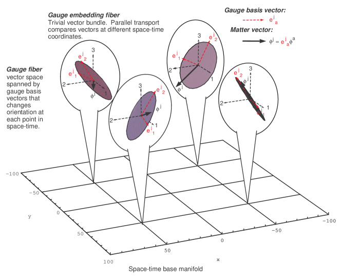
Figure 1: An ${\bf R}^{2}$-vector bundle embedded in a trivial ${\bf R}^{3}$-vector bundle. The choice of gauge determines the dotted-red basis vectors of the gauge fiber. The thick black vectors of varying length represent a real scalar matter field, which can be interpreted as a wavefunction.

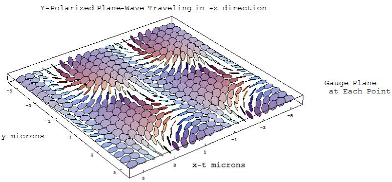
Figure 2: $\hat{y}$-polarized plane wave (24) propagating in the positive $\hat{x}$ direction. The figure corresponds to radiation with $\lambda=10.6\ \mu\rm{m}$ and intensity of $\approx 6.4$ Watts/mm².

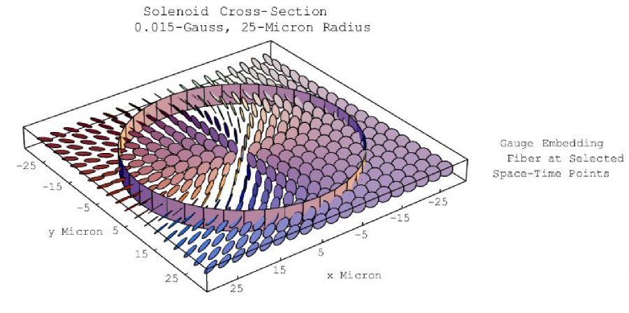
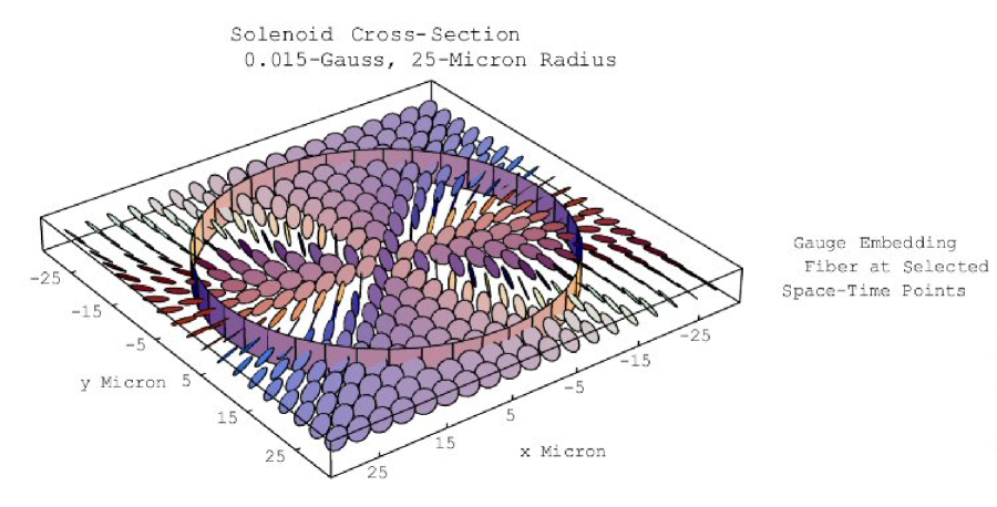
Figure 3: The cross-section of a solenoid of radius $R=25\,\mu\rm{m}$, with a magnetic field strength of $B_{o}=0.015\,\rm{Gauss}$. The diagram shows eqs. (25) and (26) for two vacuum topologies, $n=1$ in the top figure and $n=2$ in the bottom figure. The cylinder represents the solenoid boundary.

Figs. 2-7 visually represent the $SO(2)$ examples in table 2. Fig. 1 shows how to interpret figs. 2-7. Figs.  will highlight how the gauge geometry of a constant magnetic field curves the trajectory of a matter field of fixed energy.

The bubbles in fig. 1 show the trivial embedding fiber ${\bf R}^{3}$ at periodic $x$ and $y$ coordinates. The bubbles and the axis of the trivial embedding fiber, shown in fig. 1, are suppressed in the subsequent figures. The gauge-fiber basis vectors, $e^{j}_{\ 1}$ and $e^{j}_{\ 2}$, are shown as dotted, red vectors that form right angles. The disks represent the gauge-invariant, ${\bf R}^{2}$ subspace of the gauge fiber. Geometrically, the electromagnetic field is the changing orientation of the gauge fiber in the trivial, embedding fiber at different space-time points. The solid, black, vectors on the gauge fiber are the matter fields, which can be interpreted as a single-particle wavefunction.

Fig. 2 shows a $\hat{y}$-polarized plane wave (24) propagating in the $+\hat{x}$-direction. The periodicity along the $x-t$ axis corresponds to a wavelength of $\lambda=10.6\ \mu$m. The changes in the gauge-fiber orientation in the $y$-direction give the $\hat{y}$-polarization and the intensity of $6.4$ Watts/mm².

Fig. 3 shows the cross-section of a solenoid (25 and 26) with a 25-$\mu$m radius. Inside the cylinder, the $z$-directed magnetic field is $0.015$ Gauss. Outside the cylinder, the magnetic field is zero. The map (14) is surjective; the two diagrams show two different embeddings that give rise to the same magnetic field. Many of the examples in tables 1 and 2 have free parameters that give different embeddings but the same gauge fields and the same field strengths. The two diagrams in fig. 3 correspond to $n=1$ and $n=2$ topology for the vacuum outside the solenoid.

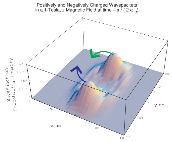
Figure 4: The wave packet used in figures 5 through 7.

Figures 5 through 7 show positive and negative wave packets at various times during a cyclotron orbit in the presence of a background, constant, z-directed magnetic field. The wave packets used for these figures, shown in fig. 4, have an energy expectation value near the second Landau level; they have the mass and apparent charge of an electron; and their cyclotron orbit has a radius of about 50 nanometers.

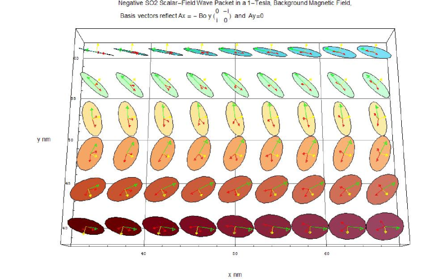
Figure 5: The green vectors are a wave packet in a 1-Tesla magnetic field orbiting the point ($x=0$, $y=50$ nm) in a counterclockwise direction. The wave packet has energy centered near the second Landau level. The light-yellow vectors show the normal to the gauge fiber. The two diagrams show two different gauge choices.

Fig. 5 shows a constant $1$-Tesla magnetic field with a negatively charged wave packet orbiting counterclockwise about the point $(x=0,y=50\ {\rm{nm}})$. The matter field is shown as a green vector. To make clear the orientation of the gauge fiber, we have added a light, yellow vector indicating the normal of the gauge fiber. The two figures show two choices of gauge. In the top figure, the basis vectors are related by parallel transport in the $y$-direction ($A_{y}=0$). In the bottom figure, the basis vectors are related by parallel transport in the $x$-direction ($A_{x}=0$). In both gauge choices, the matter-field vectors remains fixed. Using the basis vectors in the top figure, one can compare the matter vectors along the $y$-direction and observe that they are rotating counterclockwise in the momentum direction. For a positively charged wavefunction, the vectors rotate clockwise in the momentum direction. The rotating vectors may also be observed in the attached animation.

These examples raised two questions: What is the role of the basis-vector length? and What is the role of charge?

In works on gauge theory with embedded basis vector, it is generally assumed that the basis vectors are orthonormal. From the diagrams, one can see that the gauge-invariant physics is entirely captured by the orientation of the gauge fiber, in this case the ${\bf{R}}^{2}$-subspace, and the matter-field vectors. In principle, these two objects may be equally well described by any non-orthonormal basis vectors without changing the physics. The resulting gauge fields are then proportional to generators of a non-compact group. However, a traditional gauge theory of a non-compact group has completely different physics than a traditional gauge theory of a compact group [31]. This apparent contradiction is resolved by defining the Riemannian-gauge-theory action in section 6. The resolution is then discussed more carefully in section 8.

(a)

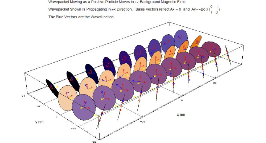
(b)

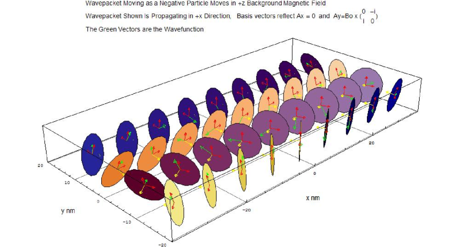
Figure 6: The first method to incorporate two matter fields with different charges. These two figures show two independent gauge fibers over the same space-time. Part (a) shows a magnetic field with positive curvature, and part (b) shows a magnetic field with negative curvature. Without an external constraint, nothing restricts the curvature of the two fibers to have any relation to each other.

Most authors writing on the geometry of gauge-fields that use basis vectors have assumed a unique coupling constant or only considered a single matter field. In this paper, we consider multiple matter fields and explore how the charge of each matter field can be varied. We found two basic methods to add multiple matter fields.

The first method establishes a separate basis vector for each matter field,

$$\phi=\phi^{a}e_{a}^{\ j}\ \ {\rm{and}}\ \ \psi=\psi^{a}E_{a}^{\ j}$$ (15)

where $e_{a}^{\ j}$ and $E_{b}^{\ j}$ are two different sets of basis vectors that describe two different gauge fibers at each space-time point. Figure 6 depicts this first method to incorporate two matter fields. The two matter fields are shown as blue and green vectors. The two parts of the figure show two independent gauge fibers over the same region of space-time. Part (a) shows a magnetic field with positive curvature, and part (b) shows a magnetic field with negative curvature. By positive curvature, we mean that a vector parallel-transported around a closed, clockwise loop in the x - y plane will be rotated clockwise in the same direction that a vector parallel-transported on the surface of a sphere sphere is rotated.

The matter field vectors of the wave packets in both parts (a) and (b) each rotate counterclockwise as one moves in the $\hat{k}$ direction. Because the curvature in parts (a) and (b) are opposite, the wave packet in part (a) will curve as a positively charged particle, and the wave packet in part (b) will curve as a negatively charged particle. Because we have changed the trajectory of part (a) compared to part (b) by temporarily redefining the sign curvature associated with the magnetic field, the matter field in part (a) rotates in the opposite direction on the gauge fiber compared to the other positive matter fields in this paper.

At this stage, there is no reason that $e_{a}^{\ j}$ and $E_{a}^{\ j}$ describe the same electromagnetic field. For example, $e_{a}^{\ j}$ could be a constant magnetic field given by eq. (27) and $E_{a}^{\ j}$ could be a plane wave given by eq. (24). There is nothing preventing one gauge fiber from representing the curvature of an electric field and the second gauge fiber from representing a zero-curvature geometry indicating no electric or magnetic field.

In order that the fields $\phi$ and $\psi$ appear to be in the same electromagnetic field, we need to constrain the curvature of the gauge fiber defined by by $e_{a}^{\ j}$ to be directly proportional to the curvature of the gauge fiber defined by $E_{a}^{\ j}$. It is the curvature of the two geometries that must be proportional, not the basis vectors. This method of incorporating multiple matter fields by placing each field on a different gauge fiber would be equivalent in general relativity to placing different particles on independent, different manifolds described by different metrics where every metric had a curvature proportional to each other.

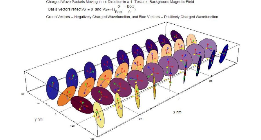
Figure 7: The second method to incorporate multiple matter fields places both matter-field vectors on the same gauge fiber.

The second method to incorporate multiple matter fields is to place the two fields, $\phi$ and $\psi$, on the same background geometry. Placing both fields on the same gauge geometry is accomplished by writing both fields in terms of the same basis vectors:

$$\phi=\phi^{a}e_{a}^{\ j}\ \ {\rm{and}}\ \ \psi=\psi^{a}e_{a}^{\ j}.$$ (16)

Figure 7 depicts this second method. The two matter fields each appear as separate blue and green vectors on the same gauge fiber.

This method has the benefit that both matter fields automatically couple to the same electric and magnetic fields. Here, the covariant derivative (10) of both fields will couple to the gauge field (11) with the same coefficient. The covariant derivative (10) has no free parameter that can be adjusted field by field.

Positive and negative charges are possible by changing the direction of rotation of the matter field on the gauge fiber. A counterclockwise or clockwise rotation as one moves in the $\hat{k}$ direction determines if the wave packet is negatively or positively charged; therefore, the two wave packets shown, although they are on the same background geometry, will be deflected in opposite directions by the magnetic field. Although we can manifest positive and negative charges, we do not have the freedom to change the magnitude of the charge.

This method of placing the two matter fields on a single gauge fiber as in figure 7 is equivalent in general relativity to placing two particles on a single manifold described by a single metric. Because the particles share a common manifold, they experience the same gravitational acceleration. In gauge geometry, because the particles share a common gauge fiber, they share a common charge magnitude. Because of the connections to general relativity, in this paper, we advocate this second method to incorporate multiple matter fields.

The geometries and the figures shown in this section have led us to reinterpret abelian gauge theory. In a traditional, abelian gauge theory, each matter field can couple with an arbitrary charge, and every matter field automatically sees the same background field. Both of these features of traditional gauge theory are problematic when the geometry is explicit. In section 6, we resolve this confusion by our definition of the action of Riemannian-gauge-theory. The examples and figures in the present section obey the equation of motion of this action. The charge uniqueness of the new action is revisited in section 7.

Description	Basis Vector
$\hat{y}$-Polarized Plane Wave $$A_{y}=2A_{o}\cos^{2}\frac{k}{2}(x-t)$$	$$e^{j}_{\ 1}=\pmatrix{e^{-i2A_{o}y}\cos\frac{k(x-t)}{2}\cr\sin\frac{k(x-t)}{2}\cr}$$ (17)
Circularly Polarized Wave $$A_{z}=A_{o}\cos^{2}(k(x-t))$$ $$A_{y}=A_{o}\sin^{2}(k(x-t))$$	$$e^{j}_{\ 1}=\left(\matrix{{f\cos(k(x-t))\exp(-i\frac{A_{o}}{f^{2}}z)}\cr{f\sin(k(x-t))\exp(-i\frac{A_{o}}{f^{2}}y)}\cr{\sqrt{1-f^{2}(\cos^{2}k(x-t)-\sin^{2}k(x-t))}}\cr}\right)$$ (18) where $f$ is any real value such that $0<f^{2}<1$.
Finite Scalar Potential $$A_{t}=\phi(\vec{x})$$	$$e^{j}_{\ 1}=\left(\matrix{{\sqrt{\frac{\phi(\vec{x})}{\kappa}}\exp(-i\,\kappa\,t)}\cr{\sqrt{1-\frac{\phi(\vec{x})}{\kappa}}}\cr}\right)$$ (19) where $0<\rm{Min}(\phi(\vec{x}))<\rm{Max}(\phi(\vec{x}))<\kappa$.
Point Charge $$A_{t}=\frac{q}{r}$$	$$e^{j}_{\ 1}(t,r)=\left(\matrix{{\sin(\kappa t)\exp(+i\frac{q}{2r\kappa}\cot(\kappa t))}\cr{\cos(\kappa t)\exp(-i\frac{q}{2r\kappa}\tan(\kappa t))}\cr}\right)$$ (20) where $\kappa$ is any real value except zero.
Solenoid: for $r<R$, $$A_{\phi}=-\frac{B_{o}r^{2}}{2}$$ $$F_{r\phi}=B_{o}r\ \ F_{xy}=B_{o}$$ for $r>R$ $$A_{\phi}=-\frac{B_{o}R^{2}}{2}\ \ F_{r\phi}=0$$	for $r<R$, $$e^{j}_{\ 1}(r,\phi)=\left(\matrix{{\sqrt{\frac{B_{o}r^{2}}{2n}}\exp(-in\phi)}\cr{\sqrt{1-\frac{B_{o}r^{2}}{2n}}}\cr}\right),$$ (21) and for, $r>R$, $$e^{j}_{\ 1}(r,\phi)=\left(\matrix{{\sqrt{\frac{B_{o}R^{2}}{2n}}\exp(-in\phi)}\cr{\sqrt{1-\frac{B_{o}R^{2}}{2n}}}\cr}\right).$$ (22) In both cases, $n$ is any nonzero integer.
Uniform Magnetic Field $$A_{x}=-B_{o}y,\ \ F_{xy}=B_{o}$$	$$e^{j}_{\ 1}(x,y)=\left(\matrix{{\sin(\kappa x)\exp(+i\frac{y\,B_{o}}{2\kappa}\cot(\kappa x))}\cr{\cos(\kappa x)\exp(-i\frac{y\,B_{o}}{2\kappa}\tan(\kappa x))}\cr}\right)$$ (23) where $\kappa$ is any real value except zero.

Table 1: Familiar $U(1)$ field strengths represented by the basis vectors of a ${\bf C}^{1}$ fiber embedded in a trivial ${\bf C}^{2}$ fiber or a trivial ${\bf C}^{3}$ fiber.

Description	Basis Vector
Plane wave $$A_{y}=A_{o}\cos(k(x-t))$$ (see fig. 2)	$\displaystyle{e^{j}_{\ 1}=\left(\matrix{{\cos A_{o}y}\cos k(x-t)\cr{\sin A_{o}y\cos k(x-t)}\cr{-\sin k(x-t)}\cr}\right)}$ $\displaystyle{e^{j}_{\ 2}=\left(\matrix{{-\sin A_{o}y}\cr{\cos A_{o}y}\cr{0}\cr}\right)}$ (24)
Solenoid For $r<R$, $$A_{\phi}=-\frac{B_{o}r^{2}}{2}$$ $$F_{r\phi}=B_{o}r$$ $$F_{xy}=B_{o}$$ For $r>R$ $$A_{\phi}=-\frac{B_{o}R^{2}}{2}$$ $$F_{r\phi}=F_{xy}=0$$ (see fig. 3)	For $r<R$, $$\matrix{{e^{j}_{\ 1}=\left(\matrix{{\cos(n\phi)\ }\cr{\sin(n\phi)\ }\cr{0}\cr}\right)}&{e^{j}_{\ 2}=\left(\matrix{{\sin(n\phi)\ \frac{B_{o}\,r^{2}}{2\,n}}\cr{-\cos(n\phi)\ \frac{B_{o}\,r^{2}}{2\,n}}\cr{\sqrt{1-(\frac{B_{o}\,r^{2}}{2\,n})^{2}}}\cr}\right)}},$$ (25) and for $r>R$, $$\matrix{{e^{j}_{\ 1}=\left(\matrix{{\cos(n\phi)\ }\cr{\sin(n\phi)\ }\cr{0}\cr}\right)}&{e^{j}_{\ 2}=\left(\matrix{{\sin(n\phi)\ \frac{B_{o}\,R^{2}}{2\,n}}\cr{-\cos(n\phi)\ \frac{B_{o}\,R^{2}}{2\,n}}\cr{\sqrt{1-(\frac{B_{o}\,R^{2}}{2\,n})^{2}}}\cr}\right)}}.$$ (26) In both cases, $n$ is any nonzero integer.
Constant Magnetic Field. $$A_{y}=B_{o}x$$ Where $|x|<a/B_{o}$. (see fig. 5)	$\displaystyle e^{j}_{\ 1}$ $\displaystyle=$ $\displaystyle\left(\matrix{{\cos y\kappa}\cr{\sin y\kappa}\cr{0}\cr}\right)$ $\displaystyle e^{j}_{\ 2}$ $\displaystyle=$ $\displaystyle\left(\matrix{{-\frac{B_{o}x}{\kappa}\sin y\kappa}\cr{\frac{B_{o}x}{\kappa}\cos y\kappa}\cr{\sqrt{1-(\frac{B_{o}x}{a})^{2}}}\cr}\right),$ (27) where $\kappa$ is any real value except zero.

Table 2: Familiar $U(1)$ field strengths represented by the basis vectors of an ${\bf R}^{2}$ fiber embedded in a trivial ${\bf R}^{3}$ fiber.

6 The Riemannian Gauge Theory Action

We construct the action for Riemannian gauge theory to be as similar as possible to the action of general relativity. We focus on writing the action in terms of inner products on the gauge fiber, which is equivalent to contracting upper indices with lower indices.

Both in general relativity and in Riemannian gauge theory, the action of the matter field is formed by inner products on the gauge fiber integrated over space-time, here taken to be four dimensional. For spinless bosons the action is

$$S_{\phi}=-\int d^{4}x\sqrt{-g}\ \left[\langle D_{\mu}\phi,D^{\mu}\phi\rangle+\langle m\phi,m\phi\rangle\right],$$ (28)

and for fermions it is

$$S_{\psi}=-\int d^{4}x\sqrt{-g}\ \left[\langle\psi,i\,\gamma^{0}\,\gamma^{\mu}\,D_{\mu}\psi\rangle+\langle\psi,m\,i\,\gamma^{0}\psi\rangle\right].$$ (29)

The factor $\sqrt{-g}$ is the square root of $-1$ times the determinant of the metric of the base manifold.

Both in general relativity and in Riemannian gauge theory, the action of the gauge fields measures the intrinsic Riemannian curvature. In general relativity, the curvature tensor (3) represents the change in a vector $V$ due to parallel transport around a loop. If the infinitesimal parallelogram starts in the $dx^{\mu}$ direction and then continues in the $dx^{\nu}$ direction, this change is

$$(V^{\prime}-V)^{\sigma}=dx^{\mu}\,dx^{\nu}\,R^{\ \ \sigma}_{\mu\nu\ \lambda}\,V^{\lambda}.$$ (30)

The tensor $R$ is the fundamental measure of intrinsic curvature. The action of general relativity

$$S_{\rm GR}=-\frac{1}{16\pi G}\int d^{4}x\sqrt{-g}\,R_{\mu\nu\lambda\sigma}\,g^{\mu\lambda}\,g^{\nu\sigma}$$ (31)

is formed from the contracted curvature tensor.

In Riemannian gauge theory, the field-strength tensor (2) also represents the change

$$(\phi^{\prime}-\phi)^{a}=i\,dx^{\mu}\,dx^{\nu}\,{F_{\mu\nu}}^{a}_{\ b}\phi^{b}$$ (32)

in a matter field $\phi$ due to parallel transport around a loop. Therefore ${F_{\mu\nu}}^{a}_{\ b}$ measures the intrinsic curvature of the gauge fiber. Both $R$ and $F$ measure intrinsic curvature, and their definitions (2) and (3) are nearly identical.

We wish to measure symmetrically the curvature of the gauge fiber and the curvature of the base manifold. To make the relationship concrete, we consider the $(4+4+n)$-dimensional total space $E_{T}$ before taking the projection $\pi_{T}=\pi_{F}\circ\pi$ which combines the projection $\pi_{F}$ for the fiber bundle of the gauge theory and the projection $\pi$ for the tangent bundle of the base manifold. We will choose the simplest total-space action that after the projection $\pi_{T}$ measures the curvature of the base manifold and of the fiber in a coordinate independent manner. We will ignore all contributions to the action which vanish under the projection $\pi_{T}$.

Given our fiber-bundle geometry, the metric of the total-space $E_{T}$ is bundle-like. A bundle-like metric $g$ on the total space satisfies $\partial_{a}g_{\mu\nu}=0$ and $g_{a\mu}=g_{\mu a}=0$ [29, 30], where the indices $a$, $b$, $c$ and $d$ still run over the fiber dimensions, and the indices $\mu$, $\nu$, $\sigma$ and $\lambda$ still run over the base manifold dimensions. In the total space $E_{T}$, the field-strength tensor is a sub-tensor of the total-space curvature tensor,

$$R_{\mu\nu\ b}^{\ \ a}=i\,{F_{\mu\nu}}^{a}_{\ b}\ \ \ {\rm{where}}\ \ \matrix{\mu,\nu&:&1\ldots 4\cr a,b&:&5\ldots 4+n\cr}.$$ (33)

This expression warrants a few notes of clarification: This equation is not a definition of our choice; rather, the equation points out that the standard curvature tensor in the total space has the gauge theory field-strength tensor as a sub-tensor. The curvature tensor of the total space is a measure of the base manifold curvature and the gauge fiber curvature. The curvature of the base manifold is measured by the curvature of the tangent bundle due to the identification of directions and lengths on the tangent bundle to directions and lengths on the base manifold. The total space $E_{T}$ includes coordinates tangent to the gauge fiber which disappear under the projection $\pi_{F}$. The coordinates and lengths of the gauge fiber are identified with the coordinates and lengths of the total space that are tangent to the fiber. Therefore, the curvature of the gauge fiber bundle is captured in the components (33) of total-space curvature tensor.

Does the total-space Ricci scalar measure the curvature in the gauge fiber? Under the fiber-like metric conditions, the Ricci tensor and the curvature scalar cannot be formed from the field strength tensor $R_{\mu\nu\ b}^{\ \ a}=iF_{\mu\nu\ b}^{\ \ a}$. In effect, because the metric components $g^{\mu a}$ vanish, both the Ricci tensor $R_{\mu\nu ab}\,g^{\mu a}$ and the curvature scalar $R_{\mu\nu ab}\,g^{\mu a}g^{\nu b}$ also vanish.

To include in the action a measure of the gauge-fiber curvature, we must use higher-order terms that do not appear in general relativity. After taking the $\pi_{T}$ projection, we find the term

$$S_{F}=\int d^{4}x\sqrt{-g}\ \frac{-1}{2\,q^{2}}{F_{\mu\nu}}^{a}_{\ b}{F^{\mu\nu}}^{b}_{\ a}$$ (34)

is the first gauge-invariant, Lorentz-invariant, higher-order measure of curvature of the gauge fiber that does not vanish due to symmetries or the block-diagonal total-space metric.

The field-strength action term (34) comes from the total-space action term quadratic in the curvature tensor. When we project this term with $\pi_{T}$ onto the base manifold, we find a new contribution to the action from the base manifold curvature:

$$S_{\rm GR-new}=\int d^{4}x\,\sqrt{-g}\,\frac{+1}{2q^{2}}\,R^{\ \ \sigma}_{\mu\nu\ \lambda}R^{\mu\nu\lambda}_{\ \ \ \sigma}.$$ (35)

The sign of this expression relative to eq. (34) is set by eq. (33). If the coupling in eq. (35) is of the same order of magnitude of the other three forces, this new term would be a very small correction to the action of general relativity.

The basis-independent action of Riemannian gauge theory is

$${S}={S}_{\phi}+S_{\psi}+{S}_{F}+S_{\rm GR}+S_{\rm GR-new}.$$ (36)

To preview the physics contained in eq. (36), we perform a small thought experiment. First, we temporarily neglect gravitational contributions and choose an orthonormal basis for the fiber $F$. Next, Narisimhan and Ramanan showed in an orthonormal basis, the gauge fields ${A_{\mu}}^{a}_{\ b}$ are $U(n)$ gauge fields. Because the action is independent of the choice of basis, this thought experiment shows the physics in eq. (36) is always that of a $U(n)$ gauge theory with a small general-relativity correction.

7 Uniqueness of the Coupling Constant

A traditional gauge theory of a compact simple non-abelian group has a unique coupling constant and discrete charges (eigenvalues). However, a traditional gauge theory of an abelian group, which has no mathematical distinction between the coupling constant and the charges, can couple to each field with a different coefficient in the covariant derivative. So there is problem of charge quantization in the traditional gauge theory of an abelian group.

Riemannian gauge theory offers a solution to this problem of traditional gauge theory. In the definition (10) of the covariant derivative, $D_{\sigma}(\phi)=e_{a}\left(\delta^{a}_{b}\partial_{\sigma}+{{{e}}}^{a}(\partial_{\sigma}e_{b})\right)\phi^{b}$, the relation $(A_{\mu})^{b}_{\ a}=i\,{{{e}}}^{b}\,(\partial_{\mu}e_{a})$ between the gauge field and the basis vectors has no adjustable parameter even in the abelian case $(A_{\mu})^{1}_{\ 1}=i\,{{{e}}}^{1}\,(\partial_{\mu}e_{1})$. This lack of an adjustable parameter is expected in the covariant derivative of an $SU(n)$ gauge theory, but it is surprising in an abelian gauge theory.

Expression (10) is not our definition. This expression follows directly from differential geometry. The physical motivation to use differential geometry is to explain the four forces in terms of symmetry and geometry.

In $U(1)$ gauge theory, the lack of an adjustable parameter in the covariant derivative (10) leads to $U(1)$ charge quantization. Every matter-field vector $\phi^{1}\,e_{1}$ on the gauge fiber $F$ couples with the same coefficient. The result is stronger than charge quantization; it is charge uniqueness. The uniqueness of the coupling in the covariant derivative arises because the matter fields are defined as vectors on a flat gauge vector bundle and because the gauge-covariant derivative is defined like the covariant derivative of Riemannian geometry. Just as geometry fixes the coefficient of $\Gamma^{\lambda}_{\mu\nu}$, so too geometry fixes the coefficient of $A_{\mu}$.

A single adjustable parameter for a particular vector bundle occurs as the coefficient of the field strength term $q^{-2}{\rm Tr}(F_{\mu\nu}F^{\mu\nu})$. This coefficient scales the action of curved gauge fiber.

We have shown that all matter-field vectors on a gauge vector bundle will couple in the covariant derivative with the same coupling constant. This unique coupling constant does not preclude positive and negative charges. Whenever one has two self-conjugate fields $\phi^{1}$ and $\phi^{2}$ of the same mass, one may form the complex field $\phi=(1/\sqrt{2})(\phi^{1}+i\phi^{2})$, which creates a particle and deletes its antiparticle; if the particle has charge $q$, then the antiparticle has charge $-q$. The particle and antiparticle correspond to the two solutions $D_{t}\phi=\pm\,i\,\omega\,\phi$. Matter-field vectors $\phi^{a}e_{a}$ with opposite charges rotate in time in opposite directions on the gauge fiber as shown in figure 7 and the attached animation. Localized matter-fields with opposite directions of rotation on a background curved gauge fiber of an electromagnetic field accelerate in opposite spatial directions.

One cannot change the charge by defining $(A_{\mu})^{a}_{\ b}=\frac{1}{q}\,i\,{{{e}}}^{1}\,(\partial_{\mu}e_{1})$. The equations of motion and the wave function evolution can be solved without ever referencing the definition (14) of $A_{\mu}$. Appendix A shows the solution of the quantum-mechanical states without defining $A_{\mu}$. The appendix connects the geometry and the curvature directly to the evolution of the wave function. The results of this calculation are depicted in figures 4 through 7. The energy fixes the rotation rate of the matter vectors in time. The canonical momentum fixes the rotation rate of the matter vectors in space. The only freedom exists in the direction of the rotation (clockwise or counterclockwise) which leads to positive and negative charges.

If the energy and momentum fix the rate of rotation, then what determines the “charge” of the wave packet? In other words, what determines the radius of the cyclotron orbit of a wave packet moving in a background magnetic field? The answer is that the trajectory is fixed by the background gauge geometry. The gauge geometry needs to be generated by some source. The efficiency with which sources curve gauge fiber is the “charge” of the theory.

As was explained in section 5, multiple independent $U(1)$ charges can occur in Riemannian gauge theory, albeit unnaturally. Using the first method described in section 5, one may introduce multiple independent $U(1)$ gauge fibers, each leading to an independent connection: $-i\,B_{\mu}={{{b}}}^{1}(\partial_{\mu}b_{1})$ and $-i\,C_{\mu}={{{c}}}^{1}(\partial_{\mu}c_{1})$. The basis vectors $b_{1}$ and $c_{1}$ are the basis vectors of two a-priori-independent, $1$-complex-dimensional gauge vector bundles $F^{(B)}$ and $F^{(C)}$. To get different charges related to the same gauge field, we need to constrain the intrinsic curvature of the two fibers $F^{(B)}$ and $F^{(C)}$ such that the connections are related by $B_{\mu}/q^{B}=C_{\mu}/q^{C}=A_{\mu}$. The geometry of two a-priori-independent gauge fibers is then constrained and expressed in terms of the variable $A_{\mu}$. Matter fields on $F^{B}$ couple with the covariant derivative $(\partial_{\mu}-iq^{B}A_{\mu})$, and matter fields on $F^{C}$ couple with the covariant derivative $(\partial_{\mu}-iq^{C}A_{\mu})$. So by putting different matter fields on different fibers, we may give them different charges.

But if all electrons, muons, and taus are represented by vectors on the same gauge fiber, then they naturally have the same electric charge. Thus Riemannian gauge theory shifts the electric charge quantization problem. Instead of wondering why so many $U(1)$ matter fields couple with the same charge $q_{e}$, we ask: Why do the quark charges differ among themselves and from the charge of the electron? Why should matter fields lie on fibers with curvatures that are related in peculiar ways? Grandly unified theories provide a natural way of constraining the curvature of different fibers.

The $SU(5)$ theory of Georgi and Glashow [19] shows how the curvature of different one-complex-dimensional fibers may be constrained to produce different $U(1)$ charges in a theory of grand unification.

We create a 5-complex-dimensional vector bundle over space-time spanned by five orthonormal basis vectors $e_{a}$. We restrict ${{{e}}}^{a}(\partial_{\mu}e_{a})=0$ to make the group $SU(5)$ instead of $U(5)$. The hypercharge gauge field $B_{\mu}$ is identified with the gauge field proportional to the diagonal generator $\lambda_{24}$

$$-iB_{\mu}=-\frac{1}{3}e^{1}(\partial_{\mu}e_{1})-\frac{1}{3}e^{2}(\partial_{\mu}e_{2})-\frac{1}{3}e^{3}(\partial_{\mu}e_{3})+\frac{1}{2}e^{4}(\partial_{\mu}e_{4})+\frac{1}{2}e^{5}(\partial_{\mu}e_{5}).$$ (37)

The matter-field covariant derivative is still $D_{\mu}\phi=e_{b}\left(\delta^{a}_{b}\partial_{\mu}+e^{a}(\partial_{\mu}e_{b})\right)\phi^{a}$, but only $\frac{1}{3}$ of the term $e^{1}(\partial_{\mu}e_{1})$ is identified as coupling to the hypercharge $B_{\mu}$. This example shows how $SU(5)$ unification constrains the curvature of different one-complex-dimensional gauge fibers so as to give different $U(1)$ charges.

Ultimately, we must appeal to a method of grand unification to explain different charges. What then are the new insights into charge quantization?

First, since Riemannian gauge theory constrains the coupling in the covariant derivative, the group $U(n)$ may be used in theories of grand unification without fear of an unconstrained $U(1)$ subgroup. Perhaps the actual unification group is $U(8)_{L}\times U(8)_{R}$.

In discussing the equations of general relativity, Einstein called the geometrical left-hand side “marble” and the material right-hand side “wood.” Riemannian geometry makes matter into marble – the matter fields are now geometrical vectors. In traditional gauge theory, the charge is a free parameter and part of the wood. Here, there is no charge, only geometry.

Third, we have found the a level of description where every object is both gauge invariant and Lorentz invariant. The gauge fiber and the matter vectors are both gauge invariant and Lorentz invariant.

Fourth, charge uniqueness is analogous to the equivalence principle. In Riemannian gauge theory, the coupling in the covariant derivative is independent of the field for the same reason that in general relativity the gravitational acceleration is independent of the mass. The equivalence principle entails that the manifold is everywhere locally flat, and therefore that every small neighborhood can be identified with a flat tangent space. Just as the tangent vectors $t_{\mu}$ describing the tangent space determine the connection (7) of the covariant derivative by the relation $\Gamma^{\alpha}_{\sigma\mu}={{{t}}}^{\alpha}(\partial_{\sigma}t_{\mu})$ without an adjustable parameter, so too the basis vectors $e_{a}$ describing the gauge fiber determine the connection (11) of the gauge-covariant derivative by the relation $(A_{\mu})^{a}_{\ b}=i{{{e}}}^{a}(\partial_{\mu}e_{b})$ without an adjustable parameter. The use of basis vectors to describe gauge fibers generalizes the equivalence principle to gauge theory. Alternatively, the observed $U(1)$ charge uniqueness is the physical principle that motivates our geometrical description of gauge theory.

8 Non-compact Gauge Groups

In section 4, we mentioned that Narasimhan and Ramanan have shown that the choice of an orthonormal basis $\langle e_{a},e_{b}\rangle=\delta_{\bar{a}b}$ on the gauge fiber $F|_{x}$ leads to an $SO(n)$ or $U(n)$ gauge theory. In eqs. (28–34), we wrote the action of a general Riemannian gauge theory in terms of basis-independent quantities. A gauge transformation is a change in the choice of basis vectors used to describe vectors in the gauge fiber. Since the action of Riemannian gauge theory is independent of the choice of basis, we can choose any linearly independent basis for the gauge fibers $F={\bf R}^{n}$ and $F={\bf C}^{n}$.

When the gauge basis vectors are allowed to be an arbitrary linearly independent set, then the symmetry group of the fiber is $GL(n,{\bf R})$ or $GL(n,{\bf C})$, and not just $SO(n)$ or $U(n)$. The action of Riemannian gauge theory and the quantities that follow from it are invariant under $GL(n,{\bf R})$ or $GL(n,{\bf C})$ gauge transformations.

In traditional gauge theory, one includes in the action every term that is renormalizable and gauge invariant In a traditional gauge theory [32, 31] of the non-compact group $GL(n,{\bf C})$, the term

$$S_{g}={m^{2}}\int d^{4}x\,\sqrt{-g}\,(D_{\mu}g)_{a\bar{b}}\,\,g^{\bar{b}c}\,(D^{\mu}g)_{c\bar{d}}\,g^{\bar{d}a}$$ (38)

occurs because it is invariant; it gives a mass to the gauge bosons associated with the non-compact generators. The physical content of this theory changes, however, when it is interpreted as a Riemannian gauge theory. In this case, as we now show, the term (38) vanishes; all the gauge bosons are massless; and the ones associated with the non-compact generators are merely gauge artifacts. The reason is that the covariant derivative of the gauge fiber metric [32, 31]

$$(D_{\mu}g)_{\bar{a}b}=\partial_{\mu}g_{\bar{a}b}-i\,(A_{\mu})^{\bar{c}}_{\ \bar{a}}g_{\bar{c}b}+i\,g_{\bar{a}c}\,(A_{\mu})^{c}_{\ b}$$ (39)

vanishes in Riemannian gauge theory. If we differentiate the definition (13) of the metric

$$\partial_{\mu}g_{\bar{a}b}=(\partial_{\mu}{\tilde{e}}_{\bar{a}}^{\ \bar{j}})\,{\tilde{e}}_{b\bar{j}}+{\tilde{e}}_{\bar{a}}^{\ \bar{j}}\,(\partial_{\mu}{\tilde{e}}_{b\bar{j}}),$$ (40)

and use the metric to raise and lower indices, e.g., ${{{e}}}^{c}_{\ j}g_{c\bar{b}}\delta^{j\bar{k}}=e_{\bar{b}}^{\ \bar{k}}$, then with an appropriate complex conjugation, we find

$$\partial_{\mu}g_{\bar{a}b}=(\partial_{\mu}{\tilde{e}}_{\bar{a}}^{\ \bar{j}})\,{\tilde{e}}^{\bar{c}}_{\ \bar{j}}\,g_{\bar{c}b}+g_{c\bar{a}}\,{\tilde{e}}^{c}_{\ j}\,(\partial_{\mu}{\tilde{e}}^{\ j}_{b}).$$ (41)

Using the definition (14) of the gauge field, we see that the covariant derivative of the metric vanishes, $(D_{\mu}g)_{\bar{a}b}=0$, and so the term (38) does not contribute to the action of the Riemannian gauge theory.

The covariant derivative of the gauge fiber metric vanishes because the gauge field and the metric are defined in terms of basis vectors. This result is reminiscent of general relativity. There the covariant derivative of the space-time metric vanishes because the connection coefficients and the metric are defined in terms of tangent basis vectors.

Freedman, Haagensen, Johnson, Latorre, and Lam [33, 34, 35]. showed a map from a local $GL(3,{\bf R})$ symmetry group onto an $SO(3)$ gauge theory. Their work on the hidden spatial-geometry of Yang-Mills theory is a special case of our Riemannian gauge theory. They identified directions on the gauge fiber $F={\bf R}^{3}$ with spatial directions on the base manifold. This identification is possible because the gauge fiber metric satisfies $(D_{\mu}g)_{ab}=0$. The resulting curved manifold with a $GL(3,{\bf R})$ local symmetry represents the geometry of the $SO(3)$ gauge fiber.

In summary, the action of Riemannian gauge theory eqs. (28 – 34) is basis independent. The choice of a non-orthonormal basis gives a larger $GL(n,{\bf R})$ or $GL(n,{\bf C})$ symmetry without adding the term (38) to the action.

9 Conclusions

Gauge theories traditionally have been defined by transformation rules for fields under a symmetry group. All gauge-invariant, renormalizable terms are included in the action. The resulting gauge theories have many parallels with Riemannian geometry. In this paper, we have constructed a gauge theory based upon Riemannian geometry, which we have called Riemannian gauge theory.

Although drawn from general relativity, the action of Riemannian gauge theory in a particular gauge is the action of traditional gauge theory. To measure the curvature of the gauge fiber, it is necessary to use a term that is quadratic in the curvature tensor. A Riemannian gauge theory with a $U(n)$ or $SO(n)$ gauge symmetry is automatically invariant under the larger gauge group $GL(n,{\bf C})$ or $GL(n,{\bf R})$; no extra terms are needed in the action.

Riemannian gauge theory offers a new insight to the problem of the quantization of charge in abelian gauge theories. The basis vectors $e_{a}$ describing the gauge fiber determine the connection (11) of the gauge-covariant derivative by the relation $(A_{\mu})^{a}_{\ b}=i{{{e}}}^{a}(\partial_{\mu}e_{b})$ without an adjustable parameter. In general relativity, all particles that move on a manifold share a common gravitational acceleration. In Riemannian gauge theory, all fields defined on a common gauge fiber share the same charge magnitude. The charge-quantization puzzle is now shifted to asking why quarks and leptons exist on independent gauge fibers related in particular ways.

Riemannian gauge theory describes the four forces in a gauge-invariant, Lorentz-invariant, geometrical form; enlarges the gauge group to a non-compact group; connects the equivalence principle with charge uniqueness; and changes the nature of the charge-quantization problem in abelian gauge theories.

Appendix A Solution of an $SO(2)$ matter field on a constant magnetic field

To solve for the states and the trajectory of a wave packet, we never have to make use of the definition (14) of $A_{\mu}$ in terms of the basis vectors. In this section, we find the states in a background magnetic field without reference to $A_{\mu}$. Instead we directly move from the geometry to the interaction with the matter fields.

We begin with the equation of motion,

$$\left((P^{l}_{\ k}\partial_{\mu})(P^{k}_{\ j}\partial^{\mu})-\delta^{l}_{\ j}m_{e}^{2}\right)e_{\ a}^{j}\phi^{a}=0$$

$$\left((P^{k}_{\ j}\partial_{\mu})(P^{l}_{\ k}\partial^{\mu})-\delta^{l}_{\ j}m_{e}^{2}\right){\tilde{e}}_{\ l}^{a}\phi_{a}=0$$

for matter fields in a background gauge field where $P$ is the projection operator and $\phi_{a}=g_{a\bar{b}}\phi^{\bar{b}}$. We wish to consider the case of an $SO(2)$ gauge theory in the presence of the constant background magnetic field (27) given in table 2.

The basis vectors are time independent. We will solve the equations of motion for modes that are time harmonic. The $SO(2)$ equation of motion is

$$\left(\matrix{e_{\ 1}^{j}&e_{\ 2}^{j}\cr}\right)\left[-\left(\matrix{\vec{\nabla}&-{{\tilde{e}}}^{2}_{\ k}\vec{\nabla}e^{k}_{\ 1}\cr{{\tilde{e}}}^{2}_{\ k}\vec{\nabla}e^{k}_{\ 1}&\vec{\nabla}\cr}\right)\cdot\left(\matrix{\vec{\nabla}&-{{\tilde{e}}}^{2}_{\ k}\vec{\nabla}e^{k}_{\ 1}\cr{{\tilde{e}}}^{2}_{\ k}\vec{\nabla}e^{k}_{\ 1}&\vec{\nabla}\cr}\right)\left(\matrix{\phi^{1}\cr\phi^{2}\cr}\right)=(\omega^{2}-m_{e}^{2})\left(\matrix{\phi^{1}\cr\phi^{2}\cr}\right)\right]$$ (42)

where we have used ${{\tilde{e}}}^{1}_{\ k}\vec{\nabla}e^{k}_{\ 2}=-{{\tilde{e}}}^{2}_{\ k}\vec{\nabla}e^{k}_{\ 1}$.

The coupled differential equation can be diagonalized into two decoupled differential equations by considering the linear combinations

$$\Phi^{1}=\frac{1}{\sqrt{2}}(\phi^{1}-i\phi^{2})$$ (43)

$$\Phi_{1}=\frac{1}{\sqrt{2}}(\phi^{1}+i\phi^{2})$$ (44)

which form two equivalent representations of our solution. We will refer to the complex vector $\Phi^{1}$ as the primary representation and or $\Phi_{1}$ as the dual representation.

Explicitly substituting the basis vectors in eq. (27) and using (43) and (44) to decouple the differential equation, we find

$$(-\nabla^{2}+2iB_{o}x\,\partial_{y}+B_{o}^{2}x^{2})\Phi^{1}=(\omega^{2}-m_{e}^{2})\Phi^{1}$$ (45)

and

$$(-\nabla^{2}-2iB_{o}x\,\partial_{y}+B_{o}^{2}x^{2})\Phi_{1}=(\omega^{2}-m_{e}^{2})\Phi_{1}.$$ (46)

Notice that these two equations happen to be complex conjugates of each other.

The solutions to this differential equation in the primary representation are

$$\Phi^{1}_{pos}=\exp(-i(\omega_{n}t-p_{z}z-p_{y}y))\Upsilon_{n}(x-\frac{p_{y}}{B_{o}})$$ (47)

$$\Phi^{1}_{neg}=\exp(+i(\omega_{n}t-p_{z}z-p_{y}y))\Upsilon_{n}(x+\frac{p_{y}}{B_{o}}),$$ (48)

and the solutions in the dual representation are

$$\Phi_{1\,pos}=\exp(+i(\omega_{n}t-p_{z}z-p_{y}y))\Upsilon_{n}(x-\frac{p_{y}}{B_{o}})$$ (49)

$$\Phi_{1\,neg}=\exp(-i(\omega_{n}t-p_{z}z-p_{y}y))\Upsilon_{n}(x+\frac{p_{y}}{B_{o}})$$ (50)

where we are using natural units and $\Upsilon_{n}$ is the $n^{\rm{th}}$ energy eigenstate of the simple harmonic oscillator. The energies are

$$\omega_{n}=+\sqrt{m_{e}^{2}+p_{z}^{2}+2|B_{o}|(n+\frac{1}{2})}.$$ (51)

Next, we use eq. (43) and (44) and rewrite these solutions in terms of the $SO(2)$ basis vectors $\phi^{1}$ and $\phi^{2}$. For positively charged particles, we have

$$\phi^{1}_{pos}={\rm{Re}}(\Phi_{1\,pos})={\rm{Re}}(\Phi^{1}_{pos})=\cos(\omega_{n}t-p_{y}y-p_{z}z)\Upsilon_{n}(x-\frac{p_{y}}{B})$$ (52)

$$\phi^{2}_{pos}={\rm{Im}}(\Phi_{1\,pos})=-{\rm{Im}}(\Phi^{1}_{pos})=\sin(\omega_{n}t-p_{y}y-p_{z}z)\Upsilon_{n}(x-\frac{p_{y}}{B}).$$ (53)

For negatively charged particles, we have

$$\phi^{1}_{neg}={\rm{Re}}(\Phi_{1\,neg})={\rm{Re}}(\Phi^{1}_{neg})=\cos(\omega_{n}t-p_{y}y-p_{z}z)\Upsilon_{n}(x+\frac{p_{y}}{B})$$ (54)

$$\phi^{2}_{neg}={\rm{Im}}(\Phi_{1\,neg})=-{\rm{Im}}(\Phi^{1}_{neg})=-\sin(\omega_{n}t-p_{y}y-p_{z}z)\Upsilon_{n}(x+\frac{p_{y}}{B}).$$ (55)

To generate figures 4 through 7, we used the non-relativistic limit of these equations, and we used a superposition of these states to form the wave packets shown in figure 4.

In this section, we never made reference to the definition (14) of the connection $A_{\mu}$. The interaction was uniquely determined by the curvature. We observe that all positively charged solutions will rotate on the plane spanned by $e^{j}_{\ 1}$ and $e^{j}_{\ 2}$ in the opposite direction from the negatively charged particles. The rotation in time is determined by the energy of the state; the rotation as one moves in space is determined by the canonical momentum. The only freedom one has is to change the direction of rotation which leads to positive and negative charges. There is no freedom left to change the magnitude of the charge.