PUPT-2027

NEIP-02-003

LPTENS-02/18

hep-th/0205171

This is a set of lectures on the gauge/string duality and non-critical strings, with a particular emphasis on the discretized, or matrix model, approach. After a general discussion of various points of view, I describe the recent generalization to four dimensional non-critical (or five dimensional critical) string theories of the matrix model approach. This yields a fully non-perturbative and explicit definition of string theories with eight (or more) supercharges that are related to four dimensional CFTs and their relevant deformations. The space-time as well as world-sheet dimensions of the supersymmetry preserving world-sheet couplings are obtained. Exact formulas for the central charge of the space-time supersymmetry algebra as a function of these couplings are calculated. They include infinite series of string perturbative contributions as well as all the non-perturbative effects. An important insight on the gauge theory side is that instantons yield a non-trivial $1/N$ expansion at strong coupling, and generate open string contributions, in addition to the familiar closed strings from Feynman diagrams. We indicate various open problems and future directions of research.

To appear in L’Unité de la Physique fondamentale: Gravité, Théories de Jauge et Cordes, Les Houches summer school 2001, Session LXXVI.

1 Introduction

String theory is an unequalled subject for the extensive techniques that it uses and the scope of ideas on which it relies. This great variety certainly is at the origin of part of the excitement in the field. Yet, it pertains to the weakest point of the theory: the lack of unifying principles, and of a consistent non-perturbative definition on which to rely. It is thus essential to stand back and to strive to find a synthesis, if only a partial one. It is with this motivation that we will discuss below the gauge theory/string theory duality. We will propose a point of view [1] that connects different approaches developed over the years. From this perspective, we are able to obtain several new results, including explicit non-perturbative definitions of many string theories and non-trivial exact formulas.

2 Many paths to the gauge/string duality

We start by discussing succinctly some of the many different facts that suggest a gauge theory/string theory duality.

2.1 Confinement

A compelling evidence for the relationship between ordinary four dimensional gauge theories like QCD and string theory is the similarity of their particle spectra. In both cases one expects to find an infinite set of resonances with masses on a Regge trajectory,

$$M_{J}^{2}\sim{J\over\alpha^{\prime}}\,\raise 2.0pt\hbox{,}$$ (1)

where $M_{J}$ is the mass of the resonance, $J$ its spin, and $\alpha^{\prime}$ sets the length scales. In the string picture, $1/\alpha^{\prime}$ is identified with the string tension. In the gauge theory picture, the dimensionless coupling constant $g_{\rm YM}^{2}$ is replaced by a scale $\Lambda$ after dimensional transmutation, and $1/\alpha^{\prime}\sim\Lambda^{2}$. Ordinary four dimensional Yang-Mills is believed to confine, and the spectrum (1) is characteristic of a confining gauge theory. Confinement is the consequence of the collimation of the chromoelectric flux lines, which generalize the ordinary Faraday flux lines of electrodynamics. The collimation can be demonstrated in the strong coupling approximation on the lattice [2], where it appears to be a consequence of the compactness of the gauge group. The string theory dual is simply the theory describing the dynamics of the tubes that the collimated flux lines form. The collimation of flux lines is interpreted in terms of a dual superconductor picture [3]. The idea is that the relevant degrees of freedom in the strongly coupled Yang-Mills theory are magnetically charged. One then assumes that those magnetic charges condense, which implies that the chromoelectric flux is squeezed into vortices, in the same way as the condensation of electric charges squeezes the magnetic field into Abrikosov vortices in an ordinary superconductor.

The chromoelectric flux vortices, or tubes, have a definite thickness of order $1/\Lambda$. The above description in terms of strings thus seems to be at best phenomenological. The well-studied fundamental strings [4] indeed have zero thickness. Equivalently, one would need a fundamental description of relativistic theories based on light electric and magnetic charges, and none were known until the proposal in [1]. Those difficulties explain why the excitement initiated in the late sixties eventually faded, and the subject remained dormant for several decades.

2.2 Large $N$

A seemingly very different argument in favor of the gauge theory/string theory duality is due to ’t Hooft [5]. In an ${\rm SU}(N)$ gauge theory, with fields transforming in the adjoint representation, the Feynman graphs can be depicted using a double-line representation corresponding to the double-index notation $A^{m}_{\bar{n}}$ for the fields. This representation makes the relationship with discretized Riemann surfaces obvious (see Figure 1). Moreover, by taking $g^{2}_{\rm YM}N$ (or equivalently after renormalization the mass scale $\Lambda$) to be an $N$-independent constant, surfaces of genus $g$ comes with a factor $1/N^{2g}$. The large $N$ expansion of ${\rm SU}(N)$ Yang-Mills theory is thus a reordering of the Feynman diagrams with respect to their topology. This shows that a perturbative discretized closed oriented string theory of coupling constant $\kappa\sim 1/N$ is equivalent to the reordered perturbative Yang-Mills theory. By perturbative, we mean that the correspondence works a priori for the contributions to the Yang-Mills path integral that can be represented in terms of Feynman diagrams. Note that the world-sheet of the string theory is embedded in the four dimensional Minkowski space, since the real-space Feynman rules imply that each vertex comes with a space-time label on which we integrate.

The weakness of the above argument is obvious: the discretized world sheets are only vaguely reminiscent of the continuous world-sheets of ordinary string theory. Only very large Feynman graphs, which have a very large number of faces, may give a good approximation to continuous world sheets. One could then argue that in the IR, which is the relevant regime for confinement, the gauge coupling is large and thus the large Feynman graphs indeed dominate. This picture is only heuristic and might at best yield an effective string theory description, similar to the one discussed in Section 2.1. We will see however that it is extremely fruitful to pursue this idea further. In a slightly different context, and with an important additional physical input, we will be able to use the ’t Hooft representation in a controlled way.

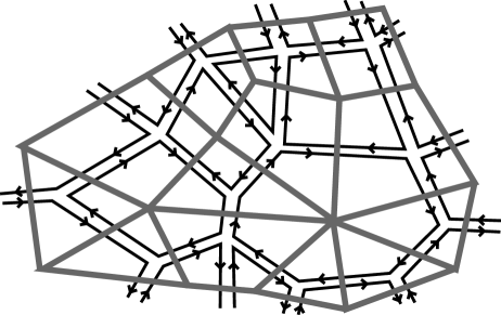
Figure 1: Part of a typical Feynman diagram in an ${\rm SU}(N)$ gauge theory, depicted in the double line representation. A dual representation (gray lines) is obtained by associating a $p$-gon to each vertex of order $p$. The $p$-gons generate an oriented discretized Riemann surface. The power of $1/N^{2}$ counts the genus of these surfaces.

2.3 D-branes

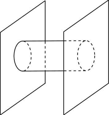
Figure 2: Interaction between D-branes. One can interpret the picture as either a one-loop diagram for an open string whose ends are stuck on the branes (this is described by a Yang-Mills theory), or as a tree diagram for a closed string propagating in the bulk (this is described by a quantum gravity theory).

Yet another argument in favor of the gauge/string correspondence has been through the use of D-branes [6]. A D$p$-brane can be described perturbatively as a $p+1$ dimensional defect in space-time on which open strings can end [7]. When $N$ D$3$-branes are put on top of each other, the low energy dynamics of the open strings is described by the ${\cal N}=4$ supersymmetric Yang-Mills theory with gauge group ${\rm SU}(N)$. On the other hand, at large $N$, the whole of the $N$ D$3$-branes is an heavy object that can be described by a classical solitonic solution in type IIB supergravity [8]. These complementary descriptions of the D-branes (see Figure 2), involving either open strings or a soliton in a closed string theory, is equivalent to the gauge/string duality. This picture can be made precise, and we refer the reader to other lectures at this school [9] in which many details about this correspondence can be found.

The above construction fits very well with the discussion of Section 2.2. The closed string coupling constant indeed turns out to be proportional to $1/N$, and $g^{2}_{\rm YM}N$ is independent of this coupling. However, it seems at first sight impossible to make it consistent with the discussion of Section 2.1. The ${\cal N}=4$ theory is indeed a conformal field theory, and thus does not confine. There is then no length scale to set the string tension. Moreover, the correspondence involves type IIB strings, which are of zero thickness and live in ten dimensions! Remarkably, it is the very fact that more than four dimensions are involved that makes the use of fundamental strings and the description of conformal gauge theories possible. Of the six additional dimensions, five play a rather technical and model-dependent rôle. They are best viewed as additional degrees of freedom on the world sheet that are necessary to account for the many “matter” fields of the ${\cal N}=4$ super Yang-Mills theory. Those fields transform under an ${\rm SO}(6)$ R-symmetry, which explains why the five dimensions actually form a 5-sphere. The other, “fifth” dimension $\phi$, is much more interesting. The form of the non-trivial five dimensional metric is actually fixed by conformal invariance to be the AdS₅ metric,

$${\rm d}s^{2}_{5}={\rm d}\phi^{2}+e^{2\phi/R}\,{\rm d}s_{4}^{2}\,,$$ (2)

where ${\rm d}s_{4}^{2}$ is the four dimensional Minkowski metric. The radius $R$ turns out to be proportional to $(g^{2}_{\rm YM}N)^{1/4}$. From (2) we see explicitly that $\phi$ can be interpreted as a renormalization group flow parameter, since a shift in $\phi$ can be absorbed in a rescaling of the Minkowski metric. The string tension varies in the fifth dimension and is set by the RG scale! The original open strings that generate the Yang-Mills dynamics are naturally attached to the brane in the far UV, $\phi\rightarrow\infty$, where all the information about the gauge theory is encoded. Confining theories can be obtained by adding some relevant operators to the ${\cal N}=4$ Yang-Mills action. The form of the metric is then in general

$${\rm d}s^{2}_{5}={\rm d}\phi^{2}+a^{2}(\phi){\rm d}s_{4}^{2}\,,$$ (3)

where the function $a(\phi)$ is well approximated by $\exp(\phi/R)$ in the UV region $\phi\rightarrow\infty$, but remains to be determined in the IR. At the confining scale $\phi=\phi_{*}\sim\ln\Lambda$, $a(\phi)$ will typically have a minimum. It is then energetically favoured for the fundamental strings to sit in this region, and this implies that they acquire an effective thickness $1/\Lambda$ from the four dimensional point of view [10].

The three aspects discussed in Section 2.1, 2.2 and 2.3 are thus fully consistent, in a subtle and interesting way. We will better understand the origin of the fifth dimension in the next subsection, but the fact that conformal field theories play a prominent rôle remains a rather weird and not very well understood feature. The discussion in Section 3 will shed some light on this part of the story.

2.4 Non-critical strings

The most direct approach to construct a string theory dual to a four dimensional field theory is to try to quantize directly the string with a target space of dimension $D=4$. Because of the quantum anomaly in the Weyl symmetry, the world sheet metric $g_{ab}$, which classically is a mere auxiliary field, does not decouple. Using world sheet diffeomorphisms, we can always put the metric in the form $g=\hat{g}e^{\phi}$, where $\hat{g}$ depends on a finite number of moduli. The conformal factor $\phi$, which is called the Liouville field, then acquires a non-trivial world sheet dynamics. When $D\leq 1$, or more precisely for a world-sheet theory of central charge $c\leq 1$, it is possible, under rather well-controlled assumptions, to work out this dynamics explicitly [11]. For example, in the case $D=1$, the classical world sheet action is

$$S={1\over 4\pi\alpha^{\prime}}\int\!{\rm d}^{2}\sigma\sqrt{g}\left(\partial_{a}X\partial^{a}X+\lambda_{0}+\alpha^{\prime}\Phi R\right)\,.$$ (4)

The world sheet scalar $X$ corresponds to the embedding coordinate and the string coupling constant is $g_{{\rm s}0}=e^{\Phi}$. A world sheet cosmological constant $\lambda_{0}$ must also be included because the Weyl symmetry is broken quantum mechanically. Integrating out $g$ then yields an action of the form

$$S={1\over 4\pi\alpha^{\prime}}\int\!{\rm d}^{2}\sigma\sqrt{\hat{g}}\left(\partial_{a}X\partial^{a}X+\partial_{a}\phi\partial^{a}\phi+T(\phi)+\alpha^{\prime}\Phi(\phi)\hat{R}\vphantom{g^{ab}\partial_{a}}\right)\,,$$ (5)

which shows that the Liouville field $\phi$ plays the rôle of a new dimension. The physics is not uniform in this new dimension because of the non-trivial “tachyon” $T$ and dilaton $\Phi$ backgrounds, which are determined by requiring world sheet conformal invariance. More details may be found in the review [12]. Unfortunately, the case $D>1$ is much more difficult and a direct analysis has never been performed. However, it can be noted [13] that the most general ansätz compatible with the symmetries of the problem, in particular with $D$-dimensional Lorentz invariance, is

$$S={1\over 4\pi\alpha^{\prime}}\int\!{\rm d}^{2}\sigma\sqrt{\hat{g}}\left(a^{2}(\phi)\partial_{a}X_{\mu}\partial^{a}X^{\mu}+\partial_{a}\phi\partial^{a}\phi+\cdots\vphantom{g^{ab}\partial_{a}}\right)\,,$$ (6)

where the dots represent various possible background fields. The main difference with the $D\leq 1$ case is that the $D+1$ dimensional metric is not flat. When $D=4$, the Liouville field is but the fifth dimension discussed in Section 2.3, and we recover in particular equation (3). For the string theory (6) to describe a gauge theory, additional consistency conditions must be satisfied. In particular, the open strings generating the Yang-Mills dynamics must live either at the horizon $a=0$ or at the point of infinite string tension $a=\infty$. The latter choice, that corresponds to a “fundamental” brane living in the far UV, seems more natural and is consistent with the discussion of Section 2.3. In either case, the open string theory will have only vector states and the zig-zag symmetry of the Wilson loops will be satisfied [13].

String theories based on actions like (6) are extremely difficult to solve. Even in the simplest case $D\leq 1$ described by (5), only a partial analysis can be given. The reason is twofold: first the world sheet theories are complicated interacting two dimensional field theories, which makes the analysis of string perturbation theory particularly involved; second the string coupling can grow due to the non-trivial dilaton background, which can altogether invalidate the use of the string perturbative framework. In spite of these daunting difficulties, the case $D\leq 1$ has actually been solved to all orders of string perturbation theory in a series of remarkable papers [14, 15, 16, 17]. The basic idea [15] is to consider a discretized version of the $D$ dimensional string theory, which turns out quite surprisingly to be easier to study than the original continuum model. The continuous world sheets are approximated by discretized surfaces made up of flat polygons of area $\ell^{2}$. The curvature is concentrated on a discrete lattice $L$ on which the vertices of the polygons lie. The discrete world sheet fields are defined at the center of the polygons, or equivalently on the dual lattice $\tilde{L}$. For example, the discrete Polyakov path integral $Z_{\rm P}(\ell)$ defining string perturbation theory based on the action (4) with the cut-off $1/\ell$ can be written

$$\hskip-28.45274ptZ_{\rm P}(a)=\sum_{h\geq 0}\int\limits_{\scriptstyle{\rm genus\ }h\atop\scriptstyle\rm world\ sheets}\hskip-17.07182pt[{\rm d}g_{ab}(\sigma){\rm d}X(\sigma)]\,e^{-S}\,{\lower 10.0pt\hbox{\vrule}}_{\,{\rm cut-off\ }1/\ell}=$$

$$\hskip 56.9055pt\sum_{h\geq 0}g_{{\rm s}0}^{2h-2}\hskip-8.5359pt\sum_{\scriptstyle{\rm genus\ }h\atop\scriptstyle{\rm lattices\ }L}\!\!\!e^{-{\lambda_{0}\ell^{2}|\tilde{L}|\over 4\pi\alpha^{\prime}}}\int\!\prod_{i\in\tilde{L}}{\rm d}X_{i}\!\!\!\prod_{\scriptstyle{\rm links\ }\langle kl\rangle\atop\scriptstyle{\rm of\ }\tilde{L}}\!\!\!\!\Delta\left(|X_{k}-X_{l}|/\smash{\sqrt{\alpha^{\prime}}}\right)\,.$$ (7)

In the above formula, $|\tilde{L}|$ represents the number of vertices of the lattice $\tilde{L}$, or equivalently the number of polygons in the discretization of the world sheet. The function $\Delta$ is a gaussian and is derived from the kinetic term for $X$ in (4). The cosmological constant $\lambda_{0}$ can a priori be renormalized, since the sum over lattices of fixed size and the integration over the $X_{i}$s can generate a counterterm proportional to $|\tilde{L}|$.

We can now use ’t Hooft’s idea described in Section 2.2. The very involved combinatorial problem corresponding to the discrete lattice sum (7) is conveniently encoded in the Feynman graph expansion of a matrix theory. Originally, ’t Hooft considered four dimensional Yang-Mills theories, but the argument is straightforwardly extended to any matrix field theory. If the matrix field theory lives in $D$ dimension(s), then the discretized world sheets are embedded in the $D$ dimensional Minkowski space. It is easy to see that the matrix theory corresponding to (7) is a quantum mechanics based on a single $N\times N$ hermitian matrix $M$, and that we have

$$e^{Z_{\rm P}(\ell)}=\int\!\left[\smash{{\rm d}^{N^{2}}}\!M(\tau)\right]\,\exp\left[-N\int\!{\rm d}\tau\,\mathop{\rm tr}\nolimits\Bigl{(}{1\over 2}\dot{M}^{2}+{1\over 2\alpha^{\prime}}M^{2}+U(M)\Bigr{)}\right].$$ (8)

The euclidean time $\tau$ corresponds to the embedding coordinate $X$ in the string theory. Terms in $M^{p}$ in the potential $U(M)$ generate $p$-gons in the discretization of the world sheets, see Figure 1. The metric on the world sheet is determined by giving an area $\ell^{2}$ to the $p$-gons. We can actually restrict ourselves to the simple potential

$$U(M)={g\over 3!}M^{3}\,.$$ (9)

More complicated potentials yield the same theory in the continuum limit. In terms of the matrix theory variables, we have

$$Z_{\rm P}(\ell)=\sum_{h\geq 0}N^{2-2h}\hskip-8.5359pt\sum_{\scriptstyle{\rm genus\ }h\atop\scriptstyle{\rm lattices\ }\tilde{L}}\!\!\!(-g)^{|\tilde{L}|}\int\!\prod_{i\in\tilde{L}}{\rm d}\tau_{i}\!\!\!\prod_{\scriptstyle{\rm links\ }\langle kl\rangle\atop\scriptstyle{\rm of\ }\tilde{L}}\!\!\!\!\Delta_{\rm E}\left(|\tau_{k}-\tau_{l}|/\smash{\sqrt{\alpha^{\prime}}}\right)\,.$$ (10)

The power of $N$ comes from the standard ’t Hooft’s analysis, and yields a string coupling $g_{{\rm s}0}=1/N$. The power $|\tilde{L}|$ of $g$ corresponds to the number of vertices in the ordinary representation of the Feynman diagrams, or equivalently to the number of polygons in the dual representation, see Figure 1. The sum is over the lattices $\tilde{L}$, which is of course equivalent to the sum over the dual lattices $L$ as in (7).

The matrix quantum mechanics (8) can be mapped onto a problem of free fermions [14], and is thus exactly solvable. In particular, the discrete Polyakov partition function, which is proportional to the radius $r$ of the embedding dimension due to translational invariance, can be calculated since it is related to the ground state energy $E(g)$,

$$E(g)=-\lim_{r\rightarrow\infty}{Z_{\rm P}(\ell)\over r}\,\cdotp$$ (11)

Any other observable of the discrete string theory could be related to quantum mechanical amplitudes in a similar way. However, and as was stressed in Section 2.2, we are still far from our goal of solving a continuum string theory. Indeed, we must find a way to implement consistently the continuum limit $\ell\rightarrow 0$. At finite $\ell$, the identification of (7) and (10) must be taken with a grain of salt, because the link factor $\Delta_{\rm E}$ is the one dimensional euclidean propagator, which is a simple exponential, unlike the gaussian $\Delta$ that corresponds to the Polyakov action. On the other hand, it is very plausible that any link factor for which a consistent continuum limit can be defined will yield the unique consistent continuum string theory.

The fact that a continuum limit can be defined for (10) relies on the non-trivial property that the average number of polygons in the relevant Feynman graphs for (8) diverges for a negative critical value of the coupling $g$ [14, 15]. Indeed, the ground state energy admits an expansion

$$E(g)=\sum_{h\geq 0}N^{2-2h}E_{h}(g)=\sum_{h\geq 0}g_{{\rm s}0}^{2h-2}E_{h}(g)\,,$$ (12)

where

$$E_{h}(g)=\sum_{k=0}^{\infty}E_{h,k}(-g)^{k}\,.$$ (13)

The numerical coefficient $E_{h,k}<0$ gives the contribution from genus $h$ surfaces with a fixed number $k$ of polygons. It is given by the terms in (10) with $|\tilde{L}|=k$. The series (13) has a finite radius of convergence which is independent of $h$, and the critical coupling corresponds to the point where it diverges [14]. This means that the large $N$ expansion of the matrix quantum mechanics breaks down at $g=g_{\rm c}$. When $g\rightarrow g_{\rm c}$, the terms with a high power of $k$, or equivalently the surfaces with a large number of polygons, dominate the sum (13). The limit $g\rightarrow g_{\rm c}$ is thus a continuum limit in which ’t Hooft’s heuristic picture of Section 2.2 becomes precise. At large $k$, $E_{h,k}$ picks up a term proportional to $(-g_{\rm c})^{-k}$, and thus we expect the contribution of surfaces of size $|\tilde{L}|$ to be proportional to $(g/g_{\rm c})^{|\tilde{L}|}\simeq\exp\left(-\smash{|\tilde{L}|(g_{\rm c}-g)}\right)$. There is actually a logarithmic correction to that formula, and $g_{\rm c}-g$ is replaced by $\epsilon$ defined by

$$g_{\rm c}-g=-\epsilon\ln\epsilon\,.$$ (14)

Comparing with (7), we get the renormalized world sheet cosmological constant

$$\lambda=4\pi\alpha^{\prime}{\epsilon\over\ell^{2}}\,\cdotp$$ (15)

This equation gives the precise relation between the coupling $g$ of the matrix quantum mechanics and the world sheet cut-off $1/\ell$. In the continuum limit, (12) naïvely suggests that $E(g)$ diverges, since the fixed genus contributions $E_{h}(g)$ themselves diverge. However, the limit can still be made consistent because the divergences are very specific, and can be compensated for by a simple multiplicative renormalization of the string coupling $g_{{\rm s}0}$ [15, 16, 17]. Indeed, we have

$$E_{h}(g)\mathop{\propto}\limits_{g\rightarrow g_{\rm c}}{1\over\epsilon^{2h-2}}\,\raise 2.0pt\hbox{,}$$ (16)

which shows that in the double scaling limit [16, 17]

$$N\rightarrow\infty\,,\quad\epsilon\rightarrow 0\,,\quad N\epsilon={\rm constant}=1/\kappa\,,$$ (17)

the ground state energy (12) has a finite limit $E_{\rm scaled}$, with an expansion of the form

$$E_{\rm scaled}=\sum_{h\geq 0}E_{h}\,\kappa^{2h-2}\,.$$ (18)

The double scaling limit (17) shows that the renormalized string coupling is

$$g_{\rm s}={1\over N\ell^{2}}={g_{{\rm s}0}\over\ell^{2}}\,\raise 2.0pt\hbox{,}$$ (19)

and thus have a non-trivial world sheet dimension two. The dimensionless coupling $\kappa$ is a combination of the genuine string coupling and of the cosmological constant,

$$\kappa={4\pi\alpha^{\prime}g_{\rm s}\over\lambda}\,\cdotp$$ (20)

The non-critical strings based on a world sheet theory of central charge $c<1$ can be treated in a similar way. The matrix quantum mechanics (8) is replaced by a simple matrix integral

$$\int\!{\rm d}^{N^{2}}\!M\,e^{-N\mathop{\rm tr}\nolimits U(M;g_{j})}$$ (21)

with a general potential

$$U(M;g_{j})={1\over 2}M^{2}+\sum_{j=3}^{p}{g_{j}\over j!}M^{j}\,.$$ (22)

By adjusting $k$ of the couplings to special values, we can go to a $k^{\rm th}$-order critical point, called the $k^{\rm th}$ Kazakov critical point, for which $c=1-3(2k-3)^{2}/(2k-1)$. The double scaling limit (17) takes the general form

$$N\rightarrow\infty\,,\quad\epsilon\rightarrow 0\,,\quad N\epsilon^{1-\gamma_{\rm str}/2}={\rm constant}\,,$$ (23)

with some exponent $\gamma_{\rm str}=-1/(k+1)$, but qualitatively the results are very similar to the $c=1$ case. All the $(p,q)$ minimal CFTs can be obtained in this way, by considering a slight generalization of (21) based on a two-matrix model. All the correlators can be studied, and the RG flows between the various theories are described by a nice mathematical structure based on the KdV hierarchy. Details can be found in [19].

Continuous world sheets with $c\leq 1$ $\displaystyle Z=\int[{\rm d}g_{ab}(\sigma){\rm d}X(\sigma)]\,e^{-S}$ $c+1$ dimensional flat target space ${\rm d}s^{2}={\rm d}\phi^{2}+{\rm d}X^{2}$
Discretized world sheets with $c\leq 1$ $\displaystyle e^{Z(\ell)}=\int\!{\rm d}^{N^{2}}\!M\,e^{-N\mathop{\rm tr}\nolimits U(M;g_{j})}$ Matrix integral with Kazakov critical points in the double scaling limit
Continuous world sheets with $c>1$ $\displaystyle Z=\int[{\rm d}g_{ab}(\sigma){\rm d}\vec{X}(\sigma)]\,e^{-S}$ $c+1$ dimensional curved target space ${\rm d}s^{2}={\rm d}\phi^{2}+a^{2}(\phi)\,{\rm d}\vec{X}^{2}$
Discretized world sheets with $c>1$ ?

Table 1: The magic square of the non-critical string theories. The continuum approach side of the $c=1$ barrier was finally cleared in 1997, but the discretized approach side remained unviolated until recently. We will try to shed some light on the material hidden behind the question mark in the following.

Let us conclude this introduction with an important remark. The simple potential (9) does not have a ground state. This means that $E(g)$ can only be defined as a sum over Feynman graphs. We could try to use another potential, for example $U(M)=gM^{4}/4!$, but the positivity of the partition function (7) implies that the coupling $g$ in (10) must be negative. As explained in details in Section 7 of the review [19], it is actually impossible to obtain a non-perturbative definition of the unitary string theories using the matrix models. The “solutions” of the $D\leq 1$ string theories thus yield the observables to all orders of perturbation theory, but not beyond. Of course, the Polyakov formulation of string theory, that was our starting point, is perturbative in nature. Equations like (11) are thus perfectly consistent and must be understood as a statement about the asymptotic perturbative series. However, it was originally expected that the powerful new formulation in terms of a matrix theory in the double scaling limit could give insights into a non-perturbative definition of string theory. The fact that this is not the case is a major drawback of the classic matrix model approach. We will have much more to say in Section 3 about this very important point of principle.

3 Four dimensional non-critical strings

The discretized approach advocated in [15] is indisputably the most fruitful to study the $D\leq 1$ string theories (5). It is then most natural to try to extend the same ideas to the $D>1$ theories (6). The first concrete results in this direction were obtained only recently by the present author [1]. The results of [1], together with the insights gained in a series of preparatory [20, 21] and subsequent [22, 23] works, strongly suggest that the discretized approach in $D>1$ (and in particular in the case $D=4$ on which we will focus) has considerable power. In particular, it provides an explicit non-perturbative definition of the $D=4$ non-critical strings, in sharp contrast with the $D\leq 1$ cases.

The first step to go from $D\leq 1$ to $D=4$ is straightforward: the $D=0$ matrix integrals (21) or $D=1$ matrix path integral (8) are replaced by $D=4$ matrix path integrals

$$\int\!\left[{\rm d}M(x)\right]\,\exp\left[-N\int\!{\rm d}^{4}x\,{\cal L}(M,\partial M)\right],$$ (24)

where $M$ represents in general a collection of $N\times N$ hermitian matrices and $\cal L$ is a lagrangian density. In the original ’t Hooft’s example [5], we have four matrices corresponding to the four components of the vector potential $A_{\mu}$, and $\cal L$ is the ${\rm SU}(N)$ Yang-Mills lagrangian with the ’t Hooft coupling $g_{\rm YM}^{2}N$ or equivalently after renormalization the dynamically generated scale $\Lambda$ chosen to be independent of $N$. The path integral (24) defines a discretized string theory with a four dimensional target space. Of course, and as stressed in Section 2.2, the real challenge is to succeed in taking the continuum limit. This was done in Section 2.4 for the simple $D\leq 1$ integrals (8) or (21) by adjusting the parameters in the interaction potential to special Kazakov critical points. However, the pure Yang-Mills path integral does not have any free parameter, and thus this procedure cannot be straightforwardly extended.

The way out of this problem was first proposed in [20]. The idea is to consider gauge theories with Higgs fields in the adjoint representation of the gauge group. The adjoint Higgs fields correspond to additional hermitian matrices $M$ on which we integrate in (24). The Higgs theory depends on couplings parametrizing the Higgs potential. Varying those couplings amounts to varying the masses of the gauge bosons, or equivalently the effective gauge coupling. It was then argued in [20] that for some special values of the Higgs couplings, that correspond to W bosons of masses of order $\Lambda$, critical points may exist. It could then be possible to define a consistent continuum limit, in strict parallel to the $D\leq 1$ cases. The consistency of those ideas were checked on a simple toy model [20]. Supersymmetry plays no rôle in the discussion, and in particular the model studied in [20] was purely bosonic. Unfortunately, and even though lattice calculations seem encouraging [24], the present-day analytical tools do not make the search for critical points in purely bosonic Yang-Mills/adjoint Higgs theories possible.

This is where supersymmetry enters the game: we do have some control on supersymmetric Yang-Mills/Higgs theories, and we can try to apply our ideas in this context. A typical example is pure ${\cal N}=2$ supersymmetric ${\rm SU}(N)$ gauge theory. The adjoint Higgs field is automatically included in this theory because it is a supersymmetric partner of the gauge bosons. Strictly speaking, this theory is parameter-free, because the Higgs coupling is related to the gauge coupling by supersymmetry, and the latter is replaced by a mass scale in the quantum theory. However, there is a freedom in the choice of the Higgs expectation values, because the Higgs potential has flat directions that are protected by a non-renormalization theorem. The path integral (24) is then parametrized by a set of boundary conditions for the Higgs field at infinity. Such parameters are called moduli of the field theory, and one can show that there are $N-1$ moduli for the pure ${\rm SU}(N)$ theory. For our purposes, the moduli will play the rôle of the couplings $g_{j}$ in the potential (22) of the $D\leq 1$ theories. In more general ${\cal N}=2$ gauge theories, one may have quark mass parameters in addition to the moduli. Mass parameters and moduli are on an equal footing in our discussion, and we will denote them collectively by ${\cal M}=\{m_{j}\}$.

There is a subtle but fundamental difference between the space of couplings $g_{j}$ for the simple matrix integrals of Section 2 and the space $\cal M$ for the gauge theories: the Yang-Mills path integrals are non-perturbatively defined for all values of the moduli or parameters, unlike the matrix integrals in $D\leq 1$. As discussed at the end of Section 2.4, this has some important consequences, because the Kazakov critical points in $D\leq 1$ always lie at the “wrong” couplings, for example $g<0$ for the integral (8) with a quartic potential. As a consequence, the $D\leq 1$ continuum string theories can only be defined in perturbation theory. We see that in four dimensions, we cannot run into this problem: we can only get non-perturbative definitions of string theories, from the non-perturbative gauge theory path integrals. The hard part is of course to find Kazakov critical points on $\cal M$.

3.1 Four dimensional CFTs as Kazakov critical points

It is well-known that there are so-called singularities on the moduli/parameter space $\cal M$ of ${\cal N}=2$ gauge theories where a non-trivial low energy physics develops [25]. For example, in the pure ${\rm SU}(N)$ case, one can adjust $p\geq 2$ moduli to special values and get an interacting CFT in the infrared [26]. The nature of such CFTs has remained rather mysterious, because the light degrees of freedom include both electric and magnetic charges, and thus a conventional local field theoretic description does not exist. Such theories are nevertheless of primary interest, because effective theories of light electric and magnetic charges are believed to play an important rôle in real world QCD, as explained at the end of Section 2.1.

The main result of our investigations is then the following:

The non-trivial CFTs on the moduli space of supersymmetric gauge theories, that can be obtained by adjusting a finite, $N$-independent, number of moduli, are the four dimensional generalizations of the Kazakov critical points. They can be used to define double scaling limits that yield string theories dual to the corresponding CFT with the possible relevant deformations.

A direct consequence of this claim is that the theories of light electric and magnetic charges can be described at a fundamental level by string theories, a result in perfect harmony with the discussion in Section 2. Moreover, many CFTs, including gauge CFTs, can be constructed in this way. For example, ${\cal N}=4$ super Yang-Mills with gauge group ${\rm SU}(p+1)$ can be obtained on the moduli space of a parent ${\cal N}=4$ theory with gauge group ${\rm SU}(N)$, by adjusting $p$ moduli. The very possibility of defining a double scaling limit automatically demonstrates that there is a string dual, whose continuous world sheets are constructed from the Feynman diagrams of the parent gauge theory.

A basic property of a Kazakov critical point is that the large $N$ expansion of the matrix theory breaks down in its vicinity. This is due to divergences at each order in $1/N$. For example, the divergence of the coefficient $E_{h}$ defined in (12) is given by (16). Those divergences are crucial, since the whole idea of the double scaling limits rely on the possibility of compensating the divergences by taking $N\rightarrow\infty$ and approaching the critical point in a correlated way. This procedure picks up the most divergent, universal, terms that correspond to the continuum string theory. A basic consequence of our claim is thus that the large $N$ expansion of ${\cal N}=2$ supersymmetric gauge theories should break down at singularities on the moduli space! More precisely, one can distinguish two classes of singularities: those that are obtained by adjusting a large number of order $N$ of moduli, and others that are obtained by adjusting a finite, $N$-independent number of moduli. Our claim implies that divergences in the large $N$ expansion must be found in the second case. This is by itself a rather strong and new statement about the behaviour of the large $N$ expansion of certain gauge theories. If the ${\cal N}=2$ parent gauge theory admits a string dual (not to be confused with the string theories produced in the double scaling limits!), it implies that the string theory does not admit a well-defined perturbation theory at the critical points.

The breakdown of the $1/N$ expansion can be given a simple interpretation. Commonly, trying to find a good approximation scheme to describe a non-trivial critical point is difficult. A typical example is $\phi^{4}$ theory in dimension $D$. The theory has two parameters, the bare mass $m$ (or “temperature”) and the bare coupling constant $g$. By adjusting the temperature, we can go to a point where we have massless degrees of freedom, and a non-trivial Ising CFT in the IR. The difficulty is that the renormalized fixed point coupling $g_{*}$ is large, and thus ordinary perturbation theory in $g$ fails. It is meaningless to try to calculate universal quantities like critical exponents as power series in $g$, since those are $g$-independent. Either the tree-level, $g$-independent contributions are exact and the corrections vanish (this occurs above the critical dimension, which is $D_{\rm c}=4$ for the Ising model, and we have a trivial fixed point $g_{*}=0$ well described by mean field theory), or the expansion parameter corresponds to a relevant operator and corrections to mean field theory are plagued by untamable IR divergencies. The critical points on the moduli space of ${\cal N}=2$ super Yang-Mills are very similar to the Ising critical point below the critical dimension, and $1/N$ is very similar to the $\phi^{4}$ coupling $g$. They are characterized by a set of critical exponents [26] that are independent of the number of colours $N$ of the parent gauge theory in which the CFT is embedded. These critical exponents cannot consistently be calculated in a $1/N$ expansion. Even the simple monopole critical points that are known to be trivial are not described consistently by the $N\rightarrow\infty$ limit of the original gauge theory, because electric-magnetic duality is not implemented naturally in this approximation scheme. Note that the argument does not apply to CFTs obtained by adjusting a large number $\sim N$ of moduli, because those are $N$-dependent, and the large $N$ expansion can then certainly be consistent.

The fact that the divergences have an IR origin implies that the string theories obtained in the double scaling limits are dual to the relevant deformations of the CFT at the critical point. Indeed, the scaling limits pick up the most IR divergent contributions, which are due to the light degrees of freedom only. This can be checked explicitly [1, 22], as we will see in Section 3.4.

Our arguments so far have been qualitative, and the reader may feel rather uncomfortable. Indeed, it is at first sight hard to imagine how to test our ideas by explicit calculations [27]. For example, one would like to compute explicitly some observables in the $1/N$ expansion, and check explicitly that the large $N$ expansion does break down at the critical point, and that the divergences are specific enough for a consistent double scaling limit to be defined. We explain below how such calculations can actually be done. This involves a rather surprising result about the large $N$ behaviour of instanton contributions at strong coupling.

3.2 Instantons and large $N$

Unlike the $D\leq 1$ matrix models, which are exactly solvable, only a small number of observables can be calculated in ${\cal N}=2$ gauge theories, following Seiberg and Witten [25, 28]. Those observables are physically very important, since they correspond to the leading term in a derivative expansion of the low energy effective action. In particular, the central charge of the supersymmetry algebra, and thus the mass of the BPS states, can be calculated exactly by using Gauss’ law. However, those observables are very special mathematically, because they pick up only a one-loop term from ordinary perturbation theory. The non-trivial physics comes entirely from an infinite series of instanton contributions.

Relevant contributions in the large $N$ limit are usually assumed to come from the sum of the Feynman graphs at each order in $1/N^{2}$ [5], as reviewed in Section 2. On the other hand, instantons are usually disregarded [29]. This is due to the fact that the instanton action is proportional to $N$ in the ’t Hooft’s scaling $g_{\rm YM}^{2}\propto 1/N$. The effects of instantons of topological charge $k$ and size $1/v$ are thus proportional, in the one-loop approximation which is exact for ${\cal N}=2$ super Yang-Mills, to

$$e^{-8\pi^{2}k/g_{\rm YM}^{2}}=\Bigl{(}{\Lambda\over v}\Bigr{)}^{kN\beta_{0}}\raise 2.0pt\hbox{,}$$ (25)

where $\beta_{0}$ is a coefficient of order $1$ given by the one-loop $\beta$ function. This formula suggests that the only smooth limit of instanton contributions when $N\rightarrow\infty$ is zero, with exponentially suppressed corrections [29]. Large instantons (small $v$), if relevant, would produce catastrophic exponentially large contributions, and if one is willing to assume that the large $N$ limit makes sense the only physically sensible conclusion seems to be that instantons are irrelevant variables. This argument is independent of supersymmetry. In real-world QCD, the ratio $\Lambda/v$ in (25) would simply be replaced by a more complicated function. In QCD, instantons of all sizes (all $v$) can potentially contribute, and this led Witten to argue that the instanton gas must vanish [29]. In Higgs theories, like ${\cal N}=2$ super Yang-Mills, the Higgs vevs introduce a natural cutoff $v$ on the size of instantons, and for $v$ large enough (“weak coupling”) the instanton gas can exist but is just negligible at large $N$. At small $v$ (“strong coupling”), we run into the same difficulties as in QCD.

The above argument would seem to imply, at least superficially, that the Seiberg-Witten observables are not suited for testing our ideas on the non-trivial behaviour of the large $N$ expansion. However, it was realized in [21] that there is a major loophole in the analysis based on (25). The point is that (25) gives the contribution at fixed instanton number $k$, whereas the full instanton contribution is given by an infinite series of the form

$$S(v/\Lambda)=\sum_{k=1}^{\infty}c_{k}\Bigl{(}{\Lambda\over v}\Bigr{)}^{kN\beta_{0}}.$$ (26)

As long as $|v|\gg|\Lambda|$, the series converges, and a term-by-term analysis makes sense. In particular, we do expect the sum $S$ to vanish exponentially at large $N$. However, at strong coupling $|v|\ll|\Lambda|$, things are entirely different because the large instantons make the sum diverge, and it is meaningless to isolate a particular term in the sum. This corresponds to the intuitive idea [29] that the instanton gas disappears. However, this does not imply that $S(v/\Lambda)$ itself is ill-defined in the strong coupling regime, because the series (25) can have a smooth analytic continuation. In some sense, instanton will transmute into something new through the process of analytic continuation. What this might be can be discovered by working out explicitly the large $N$ limit of the analytic continuation of (26) [21], and the result turns out to be extremely interesting.

3.3 A toy model example

Since we do not want to assume that the reader is familiar with the technology of the exact results in ${\cal N}=2$ gauge theories, we will discuss a simple toy example instead. Our toy example actually plays a rôle in the full calculation in the gauge theory [21, 1], but it is much simpler and nonetheless illustrates the main points discussed in Sections 3.1 and 3.2. The model is based on the equation

$$P(\sigma)=\sigma\prod_{i=1}^{N-1}(\sigma+v_{i})=\Lambda^{N}.$$ (27)

The observables are the roots of this equation. The moduli space $\cal M$ is parametrized by the $v_{i}$s. Critical points ${\rm C}_{p}$ are obtained when $p\geq 2$ roots coincide. The vicinity of ${\rm C}_{p}$ is described by the equation

$$\sigma^{p}+\sum_{k=2}^{p}t_{p-k}\sigma^{p-k}=0\,.$$ (28)

The $t_{k}$s depend on the $v_{i}$s and correspond to the $p-1$ independent relevant deformations of ${\rm C}_{p}$. They are associated with a set of critical exponents

$$\delta^{(p)}_{k}={1\over p-k}\,\cdotp$$ (29)

For example, if the most relevant operator $t_{0}$ is turned on, then the separation of the roots is of order $t_{0}^{\delta^{(p)}_{0}}$.

Let us focus on the root $\sigma_{N}$ that goes to zero in the classical, or weak coupling, limit $\Lambda/v_{i}\rightarrow 0$. In this limit, $\sigma_{N}$ is given by an instanton series of the type (26),

$$\sigma_{N}=\sum_{k=1}^{\infty}\tilde{c}_{k}\,\Lambda^{kN},$$ (30)

where the coefficients $\tilde{c}_{k}$ can be expressed in terms of the polynomial $P$,

$$\tilde{c}_{k}={1\over k!}\,\Bigl{(}{1\over\displaystyle P^{\prime}}{{\rm d}\over{\rm d}\sigma}\Bigr{)}^{k-1}\!\cdot{1\over P^{\prime}}{\lower 6.0pt\hbox{\, \vrule}}_{\,\sigma=0}.$$ (31)

The radius of convergence of (30) as a function of the distribution of the $v_{i}$s can be calculated at large $N$ with the methods of [21]. For our purposes, it is enough to consider the simple case $v_{1}=\cdots=v_{N-1}=v$. In terms of the dimensionless ratio

$$r=v/\Lambda\,,$$ (32)

the expansion (30) takes the form

$$\sigma_{N}(r)=v\sum_{k=1}^{\infty}c_{k}\,r^{-kN}$$ (33)

with $c_{1}=1$, $c_{2}=1-N$, etc…The radius of convergence of the series (33) is finite because $\sigma_{N}(r)$ has branch cuts. The branching points occur when the root $\sigma_{N}$ coincides with another root of the equation (27), and thus correspond to critical points of the type ${\rm C}_{2}$. It is elementary to show that there are $N$ critical values $r_{*}$ of $r$ given by

$$r_{*}^{N}=-{N^{N}\over(N-1)^{N-1}}$$ (34)

and for which

$$\sigma_{N}(r_{*})=\sigma_{*}=-v/N\,.$$ (35)

We see that $\sigma_{N}(r_{*})$ is of order $1/N$. There are $N$ different analytic continuations of $\sigma_{N}(r)$ for $|r|<|r_{*}|$, corresponding to the $N$ branching points (34), and which yield any of the $N$ roots of (27). To obtain the large $N$ expansion of $\sigma_{N}(r)$ for $|r|<|r_{*}|$, we write (27) as

$$\ln(1+x)+{1\over N}\ln{x\over 1+x}=\ln{1\over\rho_{\alpha}}\,\raise 2.0pt\hbox{,}$$ (36)

where $x=\sigma/v$ and $\rho_{\alpha}=e^{i\alpha}r=e^{2i\pi k/N}r$, $0\leq k\leq N-1$. The integer $k$ labels the different analytic continuations. In the $1/N$ expansion, $\alpha=2\pi k/N\in[0,2\pi[$ is actually a continuous variable. At leading order, the term proportional to $1/N$ in (36) is negligible, and we get $\sigma_{N}(r)/v=-1+1/\rho_{\alpha}+o(1)$. Corrections are obtained by substituting $x\rightarrow-1+1/\rho_{\alpha}+\Delta$ in (36) and solving for $\Delta$. The first few terms are

$${\sigma_{N}(r)\over v}=-1+{1\over\rho_{\alpha}}-{\ln(1-\rho_{\alpha})\over N\rho_{\alpha}}+{1\over 2\rho_{\alpha}N^{2}}\Bigl{[}\left(\ln(1-\rho_{\alpha})\right)^{2}+{2\rho_{\alpha}\ln(1-\rho_{\alpha})\over 1-\rho_{\alpha}}\Bigr{]}+{\cal O}(1/N^{3}).$$ (37)

The equation (37) displays all the main features of the large $N$ expansion of the analytic continuations of instanton series. The same features are found in the full gauge theory calculations [21]. First of all, it is an asymptotic series with expansion parameter $1/N$. This is very different from the series in $1/N^{2}$ that is generated by the ’t Hooft expansion in terms of Feynman diagrams. It means that open strings must be present in any string theoretic description of the ${\cal N}=2$ gauge theory. The physics underlying this fact is that the pure closed string background is singular at strong coupling. The singularity is resolved by inflating branes [30]. The open strings must be the strings that are attached to these branes [21]. A second general qualitative feature of (37) is that the contribution at each order in $1/N$ is given by a series in $1/\rho_{\alpha}$, by writing $\ln(1-\rho_{\alpha})=\ln(-\rho_{\alpha})+\ln(1-1/\rho_{\alpha})=\ln(-\rho_{\alpha})-\sum_{j=1}^{\infty}1/(j\rho_{\alpha}^{j})$. Since an instanton contributes $1/\rho_{\alpha}^{N}$, we may interpret those terms as coming from fractional instantons. The physical picture is then that instantons have disintegrated through the process of analytic continuation in the strong coupling region. The third qualitative feature is that the large $N$ expansion breaks down at $\rho_{\alpha}=1$, which corresponds to the critical point where two roots coincide.

This last feature is of course crucial for our purposes. The origin of the divergences is exactly as discussed in Section 3.1. Introducing

$$\epsilon=\rho_{\alpha}-1\,,$$ (38)

the separation of the two colliding roots goes like $\delta\sigma\propto\epsilon^{1/2}$ when $\epsilon\rightarrow 0$, the critical exponent $\delta^{(2)}_{0}=1/2$ being given by (29). However, it is straightforward to see that in the leading large $N$ approximation $\delta^{(2)}_{0}=1$. This erroneous result is obtained by noting that the formula (37) gives the large $N$ expansion of the $N-1$ roots $\sigma_{1},\ldots,\sigma_{N-1}$ for $\rho_{\alpha}>1$, a regime in which $\sigma_{N}=0$ to all orders in $1/N$ due to the exponential decrease of instantons. The divergences in the corrections to the leading approximation in (37) when $\epsilon\rightarrow 0$ signal the failure of the $1/N$ expansion to yield the correct critical exponent, as discussed in Section 3.1.

The next step is to check whether the divergences are specific enough for a double scaling limit to be defined. For this purpose, let us consider the rescaled observable

$$s=N\sigma_{N}/v$$ (39)

and the double scaling limit

$$N\rightarrow\infty\,,\quad\epsilon\rightarrow 0\,,\quad N\epsilon-\ln N={\rm constant}=1/\kappa+\ln\kappa\,.$$ (40)

By plugging in (40) into (37), and discarding terms of order $\kappa^{2}$ and higher, we get

$$s=\left(-1/\kappa-\ln\kappa-\ln N\right)+\left(-\ln(-1)+\ln\kappa+\ln N-\kappa\ln\kappa-\kappa\ln N\right)$$

$$\hphantom{s=}+\left(-\kappa\ln(-1)+\kappa\ln N+\kappa\ln\kappa\right)+\cdots$$ (41)

We have grouped together in (3.3) the terms that come from a given order in $1/N$ in (37). We see that subtle cancellations between the different terms make the result finite to the order we consider,

$$s=-1/\kappa-\ln(-1)-\kappa\ln(-1)+{\cal O}(\kappa^{2})\,.$$ (42)

It is actually very easy to see that the cancellations will work to all orders and beyond. By using the scalings (39) and (40) in the exact equation (36), we indeed obtain a non-perturbative equation determining $s$,

$$se^{s}={1\over\kappa}\,e^{-1/\kappa}\,.$$ (43)

This is an exact result for the double scaled theory, from which we can in particular derive the full asymptotic series in $\kappa$ and thus recover (42). The analogous string theoretic results that we obtain by using a gauge theory instead of the simple toy model (27) are described below.

3.4 Exact results in 4D string theory

For concreteness, let us write down explicitly some of the exact results obtained in [1]. The critical points we consider are Argyres-Douglas critical points ${\rm AD}_{p}$ which have $p-1$ relevant deformations $t_{k}$, $0\leq k\leq p-2$. The space-time dimensions of the $t_{k}$s can be deduced from the exact solution for the parent ${\cal N}=2$ supersymmetric gauge theory, and read

$$[t_{k}]_{\rm space-time}={2(p-k)\over p+2}\,\cdotp$$ (44)

The double scaling limit, similar to (23), is

$$N\rightarrow\infty\,,\quad t_{k}\rightarrow 0\,,\quad\tau_{k}=N^{1-k/n}\,t_{k}={\rm constant}\,.$$ (45)

By identifying the most relevant operator $\tau_{0}$ with the world sheet cosmological constant, and by using the reasoning in Section 2.4, equation (15) and below, we deduce that the world sheet cut-off $1/\ell$ scales as

$$\ell^{2}\sim 1/N$$ (46)

and that the world sheet dimensions are

$$[\tau_{k}]_{\rm world\ sheet}={2(p-k)\over p}\,\cdotp$$ (47)

The string theoretic central charge $z$ of the supersymmetry algebra as a function of the world sheet couplings $\tau_{k}$ reads

$$z(\gamma)={1\over 4\tau_{0}^{1/p}}\,\oint_{\gamma}{\displaystyle uT^{\prime}(u)\over\displaystyle\sqrt{1-e^{-T(u)}}}\,{\rm d}u\,,$$ (48)

with

$$T(u)=\sum_{k=0}^{p-2}\tau_{k}u^{k}+u^{p}\,.$$ (49)

The contour $\gamma$ encircles any two roots of the polynomial $T$, and corresponds to a choice of electric and magnetic charges. The formula (48) includes an infinite series of string perturbative corrections as well as all the non-perturbative contributions. It can be viewed as the “realistic” generalization of the toy model equation (43). For example, in the special case where only the most relevant operator is turned on, it is natural to introduce the coupling $\kappa=1/\tau_{0}$, to rescale $u\rightarrow\kappa^{-1/p}u$, and to consider the contours $\gamma_{jk}$ encircling the roots $u_{j}=\exp(i\pi(1+2j)/p)$ and $u_{k}$. A straightforward calculation then yields

$$z(\gamma_{jk})={p\over 4\kappa}\,\oint_{\alpha_{jk}}{\displaystyle u^{p}\,{\rm d}u\over\displaystyle\sqrt{1-e^{-(1+u^{p})/\kappa}}}=e^{i\pi(j+k+1)/p}\sin\bigl{(}\pi(j-k)/p\bigr{)}\,{\cal I}_{p}(\kappa)$$ (50)

where

$${\cal I}_{p}(\kappa)={p\over(p+1)\kappa}+\int_{0}^{1/\kappa}\Bigl{(}{\displaystyle 1\over\displaystyle\sqrt{1-e^{-x}}}-1\Bigr{)}(1-\kappa x)^{1/p}{\rm d}x.$$ (51)

The asymptotic expansion of ${\cal I}_{p}(\kappa)$ can be obtained by noting that when $x\sim 1/\kappa$, $1/\sqrt{1-\exp(-x)}-1$ is exponentially small. We thus have

$${\cal I}_{p}(\kappa)={p\over(p+1)\kappa}+\sum_{k=0}^{K}{\Gamma(k-1/p)\over\Gamma(-1/p)\Gamma(k+1)}I_{k}\,\kappa^{k}+{\cal O}(\kappa^{K+1})$$ (52)

with

$$I_{k}=\int_{0}^{\infty}\Bigl{(}{\displaystyle 1\over\displaystyle\sqrt{1-e^{-x}}}-1\Bigr{)}x^{k}\,{\rm d}x={(-1)^{k+1}\over k+1}\,\int_{0}^{1}{\left(\ln(1-t)\right)^{k+1}\over 2t^{3/2}}\,{\rm d}t.$$ (53)

The first integrals $I_{k}$ can be calculated by expanding the logarithm in powers of $t$,

$$I_{0}=2\ln 2\,,\quad I_{1}={\pi^{2}\over 6}-2(\ln 2)^{2}\,,\quad I_{2}={8(\ln 2)^{2}\over 3}-{2\pi^{2}\ln 2\over 3}+4\zeta(3)\,,$$ (54)

which gives the first string loops corrections.

An important point is that the central charge $Z$, and thus the BPS masses, of the parent gauge theory scales as [1]

$$Z\sim N^{-1/p}z\sim\ell^{2/p}\,,$$ (55)

and thus the continuum UV limit on the world sheet $\ell\rightarrow 0$ corresponds to a low energy limit of the parent gauge theory $Z\rightarrow 0$. This shows explicitly that in the double scaling limit we are left with the low energy degrees of freedom only, as was already deduced from general arguments at the end of Section 3.1.

3.5 Further insights

3.5.1 Full proofs

The consideration of the protected observables on the gauge theory side, that correspond to the central charge or equivalently to the low energy effective action, is not enough to give a full proof of the existence of double scaling limits. One should study in principle all the observables, including those with a non-trivial perturbative expansion, or equivalently the full path integral. Moreover, the heuristic picture for the appearance of a continuum string theory in the limit relies on the observation that very large Feynman graphs dominate near the critical points, as reviewed in Section 2.4. This can in principle be checked on generic amplitudes but obviously not on the BPS observables for which perturbation theory is trivial. One should also give a proof that the continuum limit does correspond to a genuine continuum string theory, a fact that is extremely difficult to check directly even in the $D\leq 1$ cases.

Unfortunately, generic amplitudes cannot be calculated in Yang-Mills theory. For that reason, it is interesting to consider simplified models that can be exactly solved. A particularly interesting one was studied in [22]. The model is a two dimensional non-linear $\sigma$ model which is a very close relative to ${\cal N}=2$ super Yang-Mills in four dimensions. It has an exactly calculable central charge with the same non-renormalization theorems as in four dimensions and the same BPS mass formula. The analysis sketched in Sections 3.1–3.4 can thus be reproduced, with qualitatively the same results (appearance of ‘fractional instantons,’ breakdown of the large $N$ expansion at critical points, possibility to define double scaling limits for which exactly known BPS amplitudes have a finite limit). Moreover, and this is the main point, the two-dimensional model is exactly solvable in the large $N$ limit: the large $N$ Feynman graphs can be explicitly summed up. It is then possible to give rigorous proofs of the existence of the double scaling limits, and to fully characterize the double scaled theories. In particular, we do obtain the expected continuum limits. Those results are extremely encouraging and strongly suggest that the scaling limits are consistent in the case of the gauge theories as well. We invite the reader to consult [22] for more details.

3.5.2 Non-perturbative non-Borel summable partition functions

As we have already emphasized, a very important point of principle is that the four dimensional double scaling limits are non-perturbative. This is to be contrasted with the classic $D\leq 1$ cases, for which the non-Borel summable observables are not defined beyond perturbation theory. We have discussed this aspect in some details in [23], where interesting mechanisms that allow for a non-perturbative definition of non-Borel summable partition functions are explicitly worked out in a class of simple theories akin to the model studied in [22].

4 Open problems

The results obtained in [1] show that a generalization of the discretized approach to four dimensional non-critical strings is possible. However, we have only scratched the surface of the subject, and many points would deserve further investigations. For example, the critical points used in [1] only correspond to one family amongst many others that can be found on the moduli space of supersymmetric gauge theories. A classification of these critical points exists [26], with an ADE pattern, and the work in [1] could certainly be generalized to the most general cases. Another interesting line of research is the study of the renormalization group flow equations between the different critical points that can be derived by using the explicit formulas of [1]. In the classic low dimensional cases, a very elegant mathematical structure emerges (generalized KdV hierarchy) when one studies the flows (see for example Sections 4 and 8 of [19]). It would be extremely interesting to discover a similar structure in the four dimensional theories. Yet another intriguing point is that the approach of [1] suggests a relationship between the analytic continuation of the sum over gauge theory instantons in the double scaling limit and sums over Riemann surfaces with boundaries which define the perturbative series of the resulting string theories. It would be worth studying if this correspondence can be proven directly by looking at the moduli space of instantons at large $N$ and large instanton number $k$. Finally, it is highly desirable to construct directly in the continuum the string theories obtained in the double scaling limits. As in the classic $D\leq 1$ case, this would provide an important consistency check of the discretized approach. Moreover, we believe that the ADE ‘exactly solvable’ four dimensional non-critical strings could play a rôle similar to the ADE minimal two dimensional CFTs, and shed considerable light into the structure of non-perturbative string theories.

References

- [1] F. Ferrari, Nucl. Phys. B 617 (2001) 348.
- [2] K. Wilson, Phys. Rev. D 10 (1974) 2445.
-
[3]
S. Mandelstam, Phys. Rep. 236 (1976) 245,
G. ’t Hooft, in High Energy Physics, Proc. European Phys. Soc. Int. Conf., A. Zichichi editor (Bologna 1976). - [4] J. Polchinski, String Theory, two volumes, Cambridge University Press 1998.
- [5] G. ’t Hooft, Nucl. Phys. B 72 (1974) 461.
-
[6]
J. Maldacena, Adv. Theor. Math. Phys. 2 (1998) 231,
S. Gubser, I.R. Klebanov and A.M. Polyakov, Phys. Lett. B 428 (1998) 105,
E. Witten, Adv. Theor. Math. Phys. 2 (1998) 253. - [7] J. Polchinski, Phys. Rev. Lett. 75 (1995) 4724.
- [8] G. Horowitz and A. Strominger, Nucl. Phys. B 360 (1991) 197.
-
[9]
J.M. Maldacena, Large field theories and
gravity, Les Houches lecture in this volume,
I.R. Klebanov, D-Branes on the Conifold and Gauge/Gravity Dualities, Les Houches lecture in this volume, hep-th/0205100. - [10] J. Polchinski and L. Susskind, String Theory and the Size of Hadrons, NSF-ITP-01-185, SU-ITP 01/56, hep-th/0112204.
-
[11]
A.M. Polyakov, Phys. Lett. B 103 (1981) 207,
T. Curtright and C. Thorn, Phys. Rev. Lett. 48 (1982) 1309,
J.-L. Gervais and A. Neuveu, Nucl. Phys. B 199 (1982) 59. - [12] P. Ginsparg and G.W. Moore, Lectures on 2D Gravity and 2D String Theory, TASI lectures 1992, hep-th/9304011.
-
[13]
A.M. Polyakov, Nucl. Phys. Proc. Suppl. 68 (1998) 1,
A.M. Polyakov, Int. J. Mod. Phys. A 14 (1999) 645. - [14] É. Brézin, C. Itzykson, G. Parisi, J.-B. Zuber, Comm. Math. Phys. 59 (1978) 35.
-
[15]
F. David, Nucl. Phys. B 257 (1985) 45,
V.A. Kazakov, Phys. Lett. B 150 (1985) 282,
J. Ambjörn, B. Durhuus and J. Fröhlich, Nucl. Phys. B 257 (1985) 433. -
[16]
É. Brézin and V.A. Kazakov, Phys. Lett. B 236 (1990) 144,
M.R. Douglas and S. Shenker, Nucl. Phys. B 355 (1990) 635,
D.J. Gross and A.A. Migdal, Phys. Rev. Lett. 64 (1990) 127. -
[17]
É. Brézin, V.A. Kazakov and Al.B. Zamolodchikov,
Nucl. Phys. B 338 (1990) 673,
D. Gross and M. Milkovic, Phys. Lett. B 238 (1990) 217,
G. Parisi, Phys. Lett. B 238 (1990) 209,
P. Ginsparg and J. Zinn-Justin, Phys. Lett. B 240 (1990) 333. - [18] I.R. Klebanov, String theory in two dimensions, lectures at the ICTP Spring School on String Theory and Quantum Gravity, Trieste, 1991, hep-th/9108019.
- [19] P. Di Francesco, P. Ginsparg and J. Zinn-Justin, Phys. Rep. 254 (1995) 1.
-
[20]
F. Ferrari, Phys. Lett. B 496 (2000) 212,
F. Ferrari, J. High Energy Phys. 6 (2001) 57. - [21] F. Ferrari, Nucl. Phys. B 612 (2001) 151.
- [22] F. Ferrari, Large and double scaling limits in two dimensions, NEIP-01-008, PUPT-1997, LPTENS-01/11, hep-th/0202002.
- [23] F. Ferrari, Non-perturbative double scaling limits, PUPT-1998, NEIP-01-009, LPTENS-02/11, hep-th/0202205.
- [24] E.H. Fradkin and S.H. Shenker, Phys. Rev. D 19 (1979) 3682.
- [25] N. Seiberg and E. Witten, Nucl. Phys. B 426 (1994) 19, erratum B 430 (1994) 485.
-
[26]
P.C. Argyres and M.R. Douglas, Nucl. Phys. B 448 (1995) 93,
T. Eguchi, K. Hori, K. Ito and S.-K. Yang, Nucl. Phys. B 471 (1996) 430. - [27] A.M. Polyakov, private communication, winter 2001.
-
[28]
P. C. Argyres and A. E. Faraggi,
Phys. Rev. Lett. 74 (1995) 3931,
A. Klemm, W. Lerche, S. Yankielowicz and S. Theisen, Phys. Lett. B 344 (1995) 169. - [29] E. Witten, Nucl. Phys. B 149 (1979) 285.
- [30] C.V. Johnson, A.W. Peet and J. Polchinski, Phys. Rev. D 61 (2000) 86001.