Spinning Q-Balls

Abstract

We present numerical evidence for the existence of spinning generalizations for non-topological Q-ball solitons in the theory of a complex scalar field with a non-renormalizable self-interaction. To the best of our knowledge, this provides the first explicit example of spinning solitons in $3+1$ dimensional Minkowski space. In addition, we find an infinite discrete family of radial excitations of non-rotating Q-balls, and construct also spinning Q-balls in $2+1$ dimensions.

I Introduction

Solitons are important ingredients of models in high energy physics. Apart from being responsible for various non-perturbative quantum phenomena, solitons are interesting in themselves, since they can be viewed as field theoretic realizations of elementary particles. It is from this viewpoint that solitons were originally introduced into physics in the context of the Skyrme model – as models of hadrons. The subsequent developments have revealed soliton solutions in many other non-linear field theories in Minkowski space, such as monopoles, vortices, sphalerons, Q-balls, etc. These solutions describe localized, particle-like objects with finite energy. Their spectra of energy and charge are typically discrete. In addition, these solutions are regular everywhere, a property which is especially appealing. So far, however, solitons have been lacking one important feature of elementary particles: the intrinsic angular momentum $J$, which is zero for all known classical solutions.

It is sensible to ask whether stationary rotating generalizations for the known static soliton solutions exist. More precisely, one is interested in finite energy, globally regular, non-radiating solutions for which the spatial integral of the $T_{0\varphi}$ component of the energy-momentum tensor,

$$J = \int T_{0\varphi}\,\mbox{d}^{3}x\;,$$ (1)

is non-vanishing. In this definition the condition of stationarity (absence of radiation) is important. Indeed, it is always possible to construct a field configuration such that $J\neq 0$ at the initial moment of time. Physically this would correspond to exciting the soliton to give it an angular momentum. However, when the time evolution starts, the received excitation will be most probably immediately radiated away, leaving behind a non-rotating object.

When talking about rotating solitons, it also seems sensible to distinguish between two types of rotation: spinning and orbiting. Spinning is associated with the intrinsic angular momentum, in analogy with the quantum-mechanical spin. Classical spin excitations, if they exist, should live in the one-soliton sector because they are excitations of an individual object. One expects that the corresponding angular momentum will assume only discrete values. Solutions describing spinning solitons in Minkowski space in $3+1$ dimensions are not known. For example, it is not known whether the ’t Hooft-Polyakov monopoles can be given classical spin. In fact, it has been shown that, at the perturbative level, monopoles do not admit stationary rotational excitations in the one-monopole sector Heusler:1998ec . This means that monopoles cannot rotate slowly, with $|J|\ll 1$. Monopoles with finite (discrete) values of $J$ are not yet excluded. However, to decide whether such solutions exist requires to go beyond perturbation theory and solving the complete coupled system of the Yang-Mills-Higgs (YMH) partial differential equations (PDEs), which is an exceedingly difficult task.

On the other hand, one can consider relative orbital motions in composite many-soliton systems. For example, one can imagine a rotating soliton-antisoliton pair balanced against mutual attraction by the centrifugal force. The spectrum of the angular momentum is then expected to be continuous. Solutions describing such orbiting solitons can actually be constructed. In the case of monopoles, for instance, there exist Taubes:1982ie ; Taubes:1982if solitonic solutions of the YMH field equations with vanishing Higgs potential in the sector with zero monopole charge. Such static, purely magnetic solutions have been explicitly constructed in Kleihaus:1999sx ; they describe monopole-antimonopole pairs balanced by a repulsive force of topological nature. Now, there is a simple way to add angular momentum to these solutions Heusler:1998ec by using the global symmetry of the field equations which mixes the Higgs field $H$ and the electric potential $\Phi$:

$$H \to H\cosh\gamma+\Phi\sinh\gamma\;,\qquad\Phi\;\to\;\Phi\cosh\gamma+H\sinh\gamma\;.$$ (2)

Applying this transformation with an arbitrary $\gamma\neq 0$ leads to solutions with an electric field. It is important to note that this also changes the angular momentum to $J\sim\sinh\gamma$ Heusler:1998ec (in fact $J=Q$, where $Q$ is the electric charge VanderBij:2001nm ). These new solutions can be interpreted as describing the system of a monopole and antimonopole rotating around their common center of mass.

Another example of systems which could be classified as orbiting solitons are rotating vortex loops. In certain models there exist vortices with stationary currents along them; ‘superconducting vortices’. One can argue Davis:1988ip ; Davis:1989ij that taking a finite piece of such a vortex, bending and closing it to form a loop, finally adding a momentum along the loop, leads to an object (vorton) described by a stationary solution of the equations of motion. The angular momentum in this case is associated with the macroscopic circulation of the current along the loop. This type of motion could be naturally classified as orbital rotation.

On the other hand, one can also consider the rotation of a straight vortex along its symmetry axis. This would correspond more closely to the notion of an intrinsic spinning rotation. Although one can show that for the Nielsen-Olesen vortex such spinning excitations do not exist, they can actually exist in other models deVega:1986eu ; Jackiw:1990aw ; Kim:1993mm ; Piette:1995mh ; Gisiger:1997vb . However, this only gives spinning solitons in $2+1$ dimensions, while their $3+1$ dimensional analogs will have infinite energy due to the infinite length of the vortex.

In summary, we are not aware of any spinning solitons in Minkowski space in $3+1$ dimensions. At the same time, such solutions are known in curved space. Indeed, there are many rotating solutions in General Relativity. In the pure gravity case they comprise the family of Kerr-Newman black holes. These are very similar to solitons, but they are not globally regular and contain a curvature singularity. There are also globally regular rotating solutions Neugebauer , but these require a source of a non-field theoretic origin. Interestingly, there exist two explicit examples of gravitating spinning solitons in pure field systems.

The first example is provided by rotating boson stars Schunk96 ; Yoshida:1997qf . These are solutions for a gravity-coupled massive complex scalar field with harmonic dependence on time and on the azimuthal angle, $\Phi(t,r,\vartheta,\varphi)=\exp(i\omega t+iN\varphi)f(r,\vartheta)$, with $N$ integer. The energy-momentum tensor is time-independent, and the Einstein equations together with the Klein-Gordon equation for $f(r,\vartheta)$ admit globally regular, stationary particle-like solutions Schunk96 . The angular momentum is quantized as $J\sim N$. The solutions with $N>0$ can be regarded as spinning excitations of the fundamental static, spherically symmetric solutions with $N=0$.

This example is instructive in the sense that it is clear ‘what rotates’: this is the phase $\omega t+N\varphi$. In this connection it is worth noting that the very notion of rotation in pure field systems is very different from that for ordinary rigid bodies. Indeed, it is meaningless to say that a given element of volume of a field system actually ‘performs revolutions’ around a given axis. Of course, one can imagine a solitonic object with a field perturbation running around it. However, such a moving perturbation will be most probably immediately radiated away. The example of boson stars thus shows that one can nevertheless have a rotating phase which is not radiated away.

In stationary rotating systems without explicit time dependence the rotation will rather be associated with certain non-linear superpositions of the multipole moments of the fields. For example, in systems with vector fields, angular momentum may be present due to a non-vanishing integral involving the Poynting vector,

$$\vec{J} = \int\vec{r}\times(\vec{E}\times\vec{B})\,\mbox{d}^{3}x\;.$$ (3)

A stationary, globally regular configuration for which this integral is non-zero would correspond to a rotating soliton.

It is possible that such solutions could exist for the SU(2) Yang-Mills fields coupled to gravity. The Einstein-Yang-Mills (EYM) field equations admit globally regular, particle like solutions Bartnik:1988am . These gravitating EYM particles are static, spherically symmetric and neutral (their purely magnetic gauge field strength decays asymptotically as $1/r^{3}$). Now, for these solutions one can perturbatively construct stationary, globally regular, axially-symmetric, slowly rotating generalizations Brodbeck:1997ek . Surprisingly, their spectrum of $J$ is continuous, as if they were composite objects, which is presumably due to the special feature of the field system consisting of only massless physical fields. Unfortunately, it is not clear at the moment whether these perturbative solutions exist also at the non-perturbative level – the analysis of VanderBij:2001nm ; Kleihaus:2002ee indicates the opposite. It is however still possible that the solitons exist, but within a more general ansatz than that considered in VanderBij:2001nm ; Kleihaus:2002ee .

In summary, spinning solitons have been found only in curved space. It is then sensible to ask if spinning solitons without gravity exist at all. In principle, it is not excluded that only gravity can support the relevant rotational degrees of freedom. In order to rule out this logical possibility, we have undertaken an attempt to construct spinning solitons in flat space.

The solitons we have chosen to ‘rotate’ are Q-balls Coleman:1985ki ; Lee:1992ax . These are solutions for a complex scalar field with a non-renormalizable self-interaction arising in some effective field theories. These solutions circumvent the standard Derrick-type argument due to having a time-dependent phase for the scalar field. In this sense they are somewhat similar to the boson stars. In the simplest spherically symmetric case the fundamental Q-ball solution was described by Coleman Coleman:1985ki . Dynamical properties of these objects have been studied in Battye:2000qj . Q-balls also appear in supersymmetric generalizations of the standard model, where one finds leptonic and baryonic Q-balls Kusenko:1997zq which may be responsible for the generation of baryon number or may be regarded as candidates for dark matter Kusenko:1998si .

In the present paper, we first recall the properties of the fundamental spherically symmetric Q-balls. In addition, we present an infinite family of their radial excitations which have not been reported in the literature before. We then turn to rotating solutions and first consider them in $2+1$ spacetime dimensions, where the problem reduces to an ordinary differential equation. Finally we consider the full problem in $3+1$ dimensions and explicitly construct solutions with angular momentum. To our knowledge, our analysis gives the first explicit example of spinning solitons in flat space.

II The Model

Let us consider a theory of a complex scalar field in $3+1$ dimensions defined by the Lagrangian

$${\mathcal{L}} = \partial_{\mu}\Phi\,\partial^{\mu}\Phi^{\ast}-U(|\Phi|)\;.$$ (4)

It is assumed that the potential $U$ has its global minimum at $\Phi=0$, where $U(0)=0$, while $U\to\infty$ for $|\Phi|\to\infty$. In addition, the potential must fulfill a particular inequality (Eq.(15)) which will be discussed below. The potential may also have local minima at some finite $|\Phi|$, as is shown in Fig. 2, but this is not necessary.

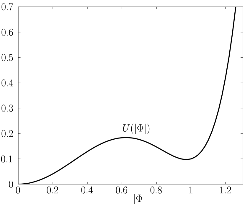
Figure 1: The qualitative shape of the potential $U(|\Phi|)$.

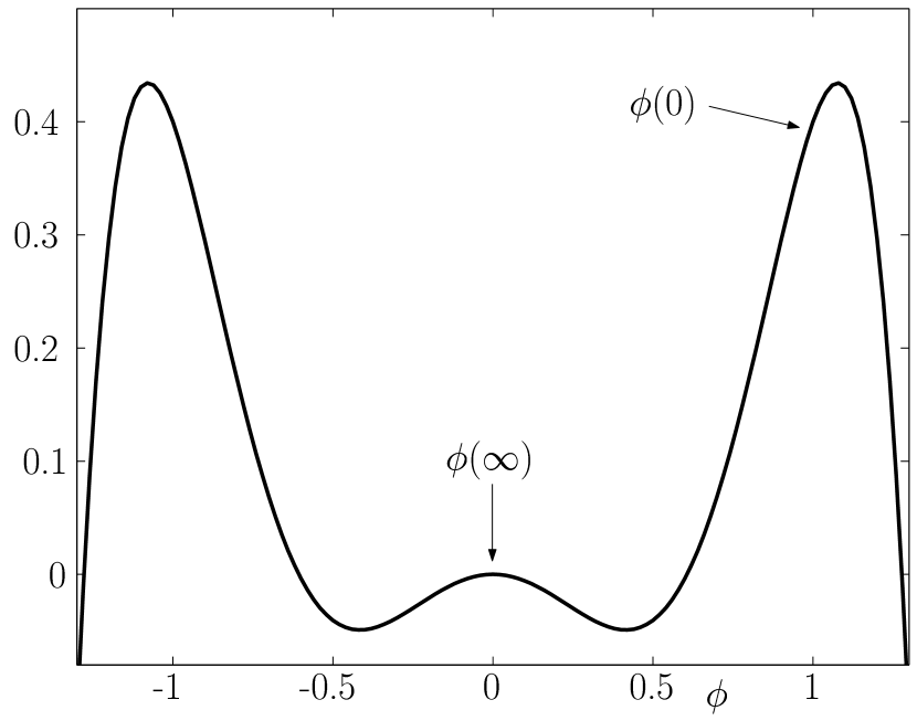
Figure 2: The effective potential $V(\phi)=\frac{1}{2}\omega^{2}\phi^{2}-U(\phi)$ in Eq. (11).

The global symmetry of the Lagrangian under $\Phi\rightarrow\Phi e^{i\alpha}$ gives rise to the conserved charge

$$Q = \frac{1}{i}\int\mbox{d}^{3}x\,(\Phi^{*}\dot{\Phi}-\Phi\dot{\Phi}^{*})\;.$$ (5)

The fundamental Q-ball solutions of the theory are minima of the energy for a given $Q$ Coleman:1985ki . Since $\Phi$ should depend on time for $Q$ to be non-vanishing, one assumes that $\Phi$ has a harmonic time dependence. In the spherically symmetric case,

$$\Phi = \phi(r)\,e^{i\omega t}\;,$$ (6)

where $\phi(r)$ is real. The potential $U(|\Phi|)=U(\phi)$ and the energy-momentum tensor,

$$T_{\mu\nu} = \partial_{\mu}\Phi\,\partial_{\nu}\Phi^{\ast}+\partial_{\nu}\Phi\,\partial_{\mu}\Phi^{\ast}-g_{\mu\nu}\,\mathcal{L}\;,$$ (7)

($g_{\mu\nu}$ being the spacetime metric) do not depend on time. The energy distribution is therefore stationary, and the total energy is

$$E = 4\pi\int_{0}^{\infty}\mbox{d}r\,r^{2}(\omega^{2}\phi^{2}+\phi^{\prime 2}+U(\phi))\;,$$ (8)

where the prime denotes differentiation with respect to $r$. The field equation,

$$0 = \frac{1}{\sqrt{-g}}\partial_{\mu}(\sqrt{-g}\,g^{\mu\nu}\partial_{\nu}\Phi)+\frac{\partial U}{\partial\Phi^{\ast}}\;,$$ (9)

reduces to

$$0 = \phi^{\prime\prime}+\frac{2}{r}\,\phi^{\prime}-\frac{\mbox{d}U(\phi)}{\mbox{d}\phi}+\omega^{2}\phi\;,$$ (10)

which is equivalent to

$$\frac{1}{2}\,\phi^{\prime 2}+\frac{1}{2}\,\omega^{2}\phi^{2}-U = \mathcal{E}-2\int_{0}^{r}\frac{\mbox{d}r}{r}\,\phi^{\prime 2}\;.$$ (11)

This effectively describes a particle moving with friction in the one dimensional potential

$$V(\phi)=\frac{1}{2}\,\omega^{2}\phi^{2}-U(\phi)\;.$$ (12)

$\mathcal{E}$ is an integration constant playing the role of the total ‘effective energy’. It is essential that the potential $V(\phi)$ should have the qualitative shape shown in Fig. 2, which is possible if the following conditions are fulfilled. First, since $V^{\prime\prime}(0)<0$, it follows that $\omega^{2}$ should not be too large:

$$\omega^{2} < \omega^{2}_{\max}\;\equiv\;U^{\prime\prime}(0)\;.$$ (13)

On the other hand, $\omega^{2}$ should not be too small, since otherwise $V(\phi)$ will be always negative. $V(\phi)$ will become positive for some non-zero $\phi$, as is shown in Fig. 2, if only

$$\omega^{2} > \omega^{2}_{\min}\;\equiv\;\min_{\phi}({2U(\phi)}/{\phi^{2}})\;,$$ (14)

where the minimum is taken over all values of $\phi$. For the potential $U(\phi)$ it is necessary that

$$U^{\prime\prime}(0) > \min_{\phi}({2U(\phi)}/{\phi^{2}})\;,$$ (15)

since only then the set of values of $\omega^{2}$ will be non-empty. The only possible renormalizable interaction in the theory, $U=\frac{1}{2}\mu^{2}|\Phi|^{2}+\lambda|\Phi|^{4}$, does not obey this condition. Thus non-renormalizable potentials have to be considered Coleman:1985ki . For example, for the potential

$$U(\phi) = \lambda(\phi^{6}-a\phi^{4}+b\phi^{2})$$ (16)

the condition (15) is fulfilled for any positive $\lambda$, $a$, $b$, and $U(\phi)$ will have a global minimum at $\phi=0$ if $b>a^{2}/4$. We use this model potential with $\lambda=1$, $a=2$ and $b=1.1$ in all our calculations below, in which case the conditions (13), (14) require that $0.2\leq\omega^{2}\leq 2.2$.

III Fundamental Q-balls and their radial excitations

If conditions (13)–(15) are fulfilled, then the field equation admits globally regular solutions $\phi(r)$ with finite energy Coleman:1985ki . The necessary condition for the energy (8) to be finite is that the potential $U\to 0$ for large $r$, and therefore $\phi\to 0$ as $r\to\infty$. Linearizing Eq. (10) around $\phi=0$, one finds that asymptotically

$$\phi = \frac{A}{r}\exp\left\{-\sqrt{(U^{\prime\prime}(0)-\omega^{2})}\,r\right\}\left(1+O(1/r)\right)\;,$$ (17)

where $A$ is an integration constant. In view of (13) the argument of the exponent is real and negative, and so $\phi$ approaches zero exponentially fast.

Solutions must also be regular at the origin of the coordinate system, $r=0$. Since $r=0$ is the regular singular point of Eq. (10), the solution will only be regular if it belongs to the ‘stable manifold’ characterized by the local Taylor expansion in the vicinity of $r=0$,

$$\phi(r) = \phi_{0}+(U^{\prime}(\phi_{0})-\omega^{2}\phi_{0})\,r^{2}+O(r^{4})\;,$$ (18)

where $\phi_{0}$ is an integration constant.

Extending the two local solutions (17), (18) to finite values of $r$ and requiring that $\phi$ and $\phi^{\prime}$ for both solutions agree at some $r=r_{0}$, yields two conditions for the free parameters $A$ and $\phi_{0}$. Resolving these conditions determines a globally regular solution in the interval $r\in[0,\infty)$. In fact, in this way an infinite discrete family of globally regular solutions parametrized by the number $n=0,1,2,\ldots$ of nodes of $\phi$ is obtained. The existence of these solutions can be illustrated by the following qualitative argument.

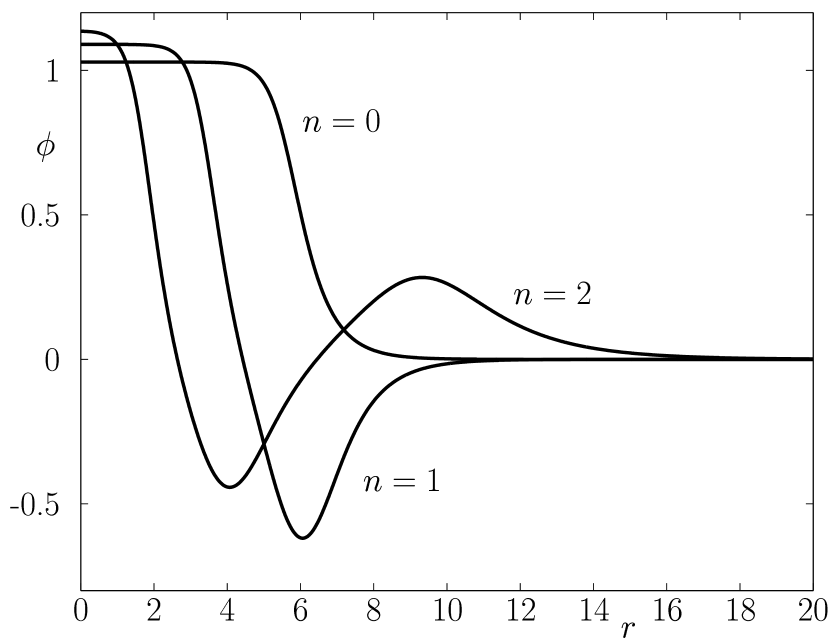
Figure 3: The profile of $\phi(r)$ for the fundamental Q-ball solution and its first two radial excitations.

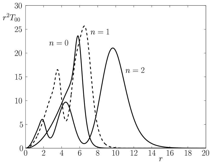
Figure 4: The radial energy density $r^{2}T_{00}$ for the fundamental Q-ball and its first two excitations.

The parameter $\phi_{0}$ in (18) is the coordinate of the ‘particle’ at the initial moment of ‘time’, $r=0$, when the particle velocity is zero, $\phi^{\prime}(0)=0$. The particle therefore starts its motion from some point on the curve $V(\phi)$ in Fig. 2, with the total effective energy $\mathcal{E}$ being equal to its potential energy. Then it moves to the right, dissipating some of its energy along its way. For $r\to\infty$, the particle must end up at the local maximum of the potential $V$ (at $\phi=0$) with the total effective energy being zero. This can be achieved by fine-tuning the initial position of the particle, $\phi_{0}$. If $V(\phi_{0})<0$, the effective energy of the particle will always be negative, and therefore it will not be able to end up in a configuration with zero energy. On the other hand, if $\phi_{0}$ is such that the particle starts very close to the absolute maximum of $V$, then it will stay there for a long ‘time’ $r$, during which period the dissipation term in (11), which is $\sim 1/r$, will become very small. As a result, when the particle will eventually start moving, its energy will be too large, and so it will ‘overshoot’ the position with zero energy. By continuity, there is a value $\phi_{0}$ for which the total effective energy (the right hand side in (11)) is exactly zero for $r\to\infty$, and so the particle will travel from $\phi(0)=\phi_{0}$ to $\phi(\infty)=0$ Coleman:1985ki .

Next, one can fine-tune $\phi_{0}$ such that the initial energy $V(\phi_{0})$ is slightly too large, so that the particle first overshoots the $\phi=0$ position, but then it hits the barrier from the other side, bounces back and dissipates just enough energy to finally arrive at $\phi=0$ with zero energy. This will give a solution with one node of $\phi(r)$ in the interval $r\in[0,\infty)$. Similarly one can obtain solutions with $n>1$. To recapitulate, for each $\omega^{2}$ subject to (13), (14) there is a solution to Eq. (10) for which $\phi(r)$ smoothly interpolates between some finite value at the origin and zero value at infinity, crossing zero $n$ times in between. We shall call solutions with $n=0$ fundamental Q-balls. Solutions with $n>0$ are the radial Q-ball excitations. The family of Q-ball solutions can thus be parameterized by $(\omega,n)$.

As the frequency $\omega$ changes in the range $\omega_{\min}^{2}<\omega^{2}<\omega_{\max}^{2}$, the charge

$$Q(\omega) = 8\pi\omega\int_{0}^{\infty}\mbox{d}r\,r^{2}\phi^{2}$$ (19)

changes from $Q(\omega_{\min})=\pm\infty$ (depending on the sign of $\omega$) to $Q(\omega_{\max})=0$. This can be understood as follows. For $\omega^{2}\to\omega_{\max}^{2}$ the minimum of the effective potential $V(\phi)$ becomes more and more shallow and moves closer and closer to $\phi=0$. This implies that the range of values of the solution $\phi(r)$ diminishes and the interval of $r$ in which $\phi(r)$ is not constant decreases. Q-balls therefore ‘shrink’ in this limit, and the integral (19) tends to zero. In the opposite limit, $\omega^{2}\to\omega_{\min}^{2}$, Q-balls become large, and their charge tends to infinity.

These considerations imply that instead of $\omega$ one can choose the charge $Q$ as the independent parameter. Spherically symmetric $Q$-balls therefore comprise a two-parameter family labeled by $(Q,n)$, where the charge $-\infty<Q<\infty$ and the ‘excitation number’ $n=0,1,2,\ldots$. In Figs. 3–4 the profiles of the fundamental solution and its first two radial excitations are shown for $Q=1100$. As one can see from the shape of the radial energy density, the $n$-th solution has the structure of $n+1$ concentric spherical layers of energy.

IV Spinning Q-vortices.

Our aim now is to show that Q-balls admit spinning generalizations. For this we modify the ansatz (6) according to

$$\Phi = \phi(r,\vartheta)\,e^{i\omega t+iN\varphi}\;,$$ (20)

where $N$ is an integer. This produces a non-zero component of the angular momentum along the $z$-axis. Inserting this ansatz into the field equation (9), the problem reduces to a non-linear PDE for the function $\phi(r,\vartheta)$. Before we start solving this equation, however, it is instructive to consider a simpler system which effectively lives in $2+1$ dimensions. Then the problem reduces to an ordinary differential equation (ODE).

Let us pass from spherical coordinates $(t,r,\vartheta,\varphi)$ to polar coordinates $(t,\rho,z,\varphi)$, and then assume that the field does not depend on $z$:

$$\Phi = \phi(\rho)\,e^{i\omega t+iN\varphi}\;.$$ (21)

This will correspond to a vortex-type configuration, invariant under translations along the $z$-axis. The energy per unit vortex length is

$$E = 2\pi\int_{0}^{\infty}\rho\,\left(\omega^{2}\phi^{2}+\phi^{\prime 2}+\frac{N^{2}}{\rho^{2}}\,\phi^{2}+U(\phi)\right)\,\mbox{d}\rho\;.$$ (22)

If $N\neq 0$, the vortex will rotate around the $z$-axis, its angular momentum per unit length being given by

$$J = \int T_{0\varphi}\,\rho\,\mbox{d}\rho\,\mbox{d}\varphi\;=\;4\pi\omega N\int_{0}^{\infty}\rho\,\phi^{2}\,\mbox{d}\rho\;\equiv\;NQ\;,$$ (23)

where $Q$ is the charge per unit length. The field equation now reads

$$0 = \phi^{\prime\prime}+\frac{1}{\rho}\,\phi^{\prime}-\frac{N^{2}}{\rho^{2}}\,\phi-\frac{\mbox{d}U(\phi)}{\mbox{d}\phi}+\omega^{2}\phi\;.$$ (24)

For $N=0$ this reduces to (10), with the replacement $2/r\to 1/\rho$ in the friction term. All arguments above still apply, hence we conclude that there exist globally regular ‘Q-vortex’ solutions and their radial excitations with finite energy per unit length. These solutions display the behaviors qualitatively similar to those shown in Fig. 4.

Let us now consider solutions with $N>0$. As can be seen from (22), the energy for such solutions will be finite if only $\phi(0)=0$, such that the boundary condition for small $\rho$ is now different. The power series solution to (24) in the vicinity of $\rho=0$ reads

$$\phi = B\rho^{N}+O(\rho^{N+1})\;,$$ (25)

where $B$ is an integration constant. The asymptotic behavior for large $\rho$ is

$$\phi = \frac{A}{\sqrt{\rho}}\exp\left\{-\sqrt{(U^{\prime\prime}(0)-\omega^{2})}\,\rho\right\}\left(1+O(1/\rho)\right)\;.$$ (26)

One can use essentially the same qualitative considerations as in the preceding section to argue that globally regular solutions to (24) with such boundary conditions exist, provided that $\omega$ still fulfills conditions (13), (14). These solutions can be obtained by numerically extending the asymptotics (25), (26) to finite values of $\rho$ and adjusting the free parameters $A$, $B$ to fulfill the matching conditions at some $\rho=\rho_{0}$.

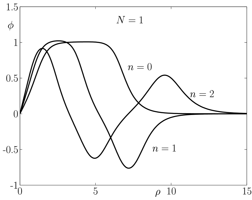
Figure 5: The spinning $N=1$ fundamental Q-vortex solution and its first two radial excitations; $Q=150$.

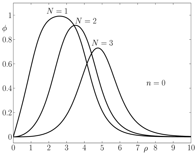
Figure 6: The first three spinning excitations of the fundamental Q-vortex solution; $Q=60$.

The conclusion is that there exists a family of globally regular spinning Q-vortex solutions. These solutions can be labeled by $(Q,n,N)$, where $Q$ is the charge per unit vortex length, $n=0,1,2,\ldots$ is the radial ‘quantum’ number (the number of nodes of $\phi(\rho)$) and $N=0,1,2,\ldots$ is the rotational ‘quantum’ number. For fixed $Q$, the energy per unit length, $E(Q,n,N)$, depends on both $n$ and $N$, while the angular momentum is determined only by the value of $N$ as $J=NQ$. The profiles of $\phi(\rho)$ for several low-lying excitations of the fundamental Q-vortex are shown in Figs. 6–6.

V Spinning Q-balls

Having considered the simpler problem in $2+1$ dimensions, we now return to our main task of finding rotating Q-ball solutions in $3+1$ dimensions. Although, these two cases are qualitatively somewhat similar, the $3+1$ dimensional problem is technically more involved, since it requires solving a non-linear PDE. With $\Phi=\phi(r,\vartheta)\;e^{i\omega t+iN\varphi}$ the field equation reduces to

$$\left(\frac{\partial^{2}}{\partial r^{2}}+\frac{2}{r}\frac{\partial}{\partial r}+\frac{1}{r^{2}}\frac{\partial^{2}}{\partial\vartheta^{2}}+\frac{\cos\vartheta}{r^{2}\sin\vartheta}\frac{\partial}{\partial\vartheta}-\frac{N^{2}}{r^{2}\sin^{2}\vartheta}+\omega^{2}\right)\phi = \frac{\mbox{d}U(\phi)}{\mbox{d}\phi}\;.$$ (27)

The energy, $E=\int T_{00}\,\mbox{d}^{3}x$, reads

$$E = 2\pi\int_{0}^{\infty}\mbox{d}r\,r^{2}\,\int_{0}^{\pi}\mbox{d}\vartheta\,\sin\vartheta\left(\omega^{2}\phi^{2}+(\partial_{r}\phi)^{2}+\frac{1}{r^{2}}(\partial_{\vartheta}\phi)^{2}+\frac{N^{2}\phi^{2}}{r^{2}\sin^{2}\vartheta}+U(\phi)\right)\;,$$ (28)

the charge

$$Q = 2\omega\int\phi^{2}\,\mbox{d}^{3}x\;=\;4\pi\omega\int_{0}^{\infty}\mbox{d}r\,r^{2}\int_{0}^{\pi}\mbox{d}\vartheta\,\sin\vartheta\,\phi^{2}\;,$$ (29)

and the angular momentum

$$J = \int T_{0\varphi}\,\mbox{d}^{3}x\;=\;NQ\;.$$ (30)

Finiteness of the energy requires that

$$\phi \to 0\qquad\text{as}\quad r\;\to\;0\text{ or }\infty\;.$$ (31)

The asymptotic behavior of the solutions in these limits can be easily determined, since for small $\phi$ one has $\mbox{d}U/\mbox{d}\phi\approx U^{\prime\prime}(0)\,\phi$, such that equation (27) actually becomes linear. The variables then separate, implying that the most general asymptotic solution has the form

$$\phi(r,\vartheta) = \sum_{l=N}^{\infty}f_{l}(r)\,P^{N}_{l}(\cos\vartheta)\;.$$ (32)

Here, $P^{N}_{l}(\cos\vartheta)$ are the associated Legendre functions. At the origin, the radial amplitudes $f_{l}(r)$ are

$$f_{l}(r) = C_{l}\,r^{l}+O(r^{l+1})\;,$$ (33)

while at infinity

$$f_{l}(r) = \frac{A_{l}}{r}\,\exp\left\{-\sqrt{(U^{\prime\prime}(0)-\omega^{2})}\,r\right\}\left(1+O(1/r)\right)\;,$$ (34)

$C_{l}$ and $A_{l}$ denoting integration constants.

Eqs. (32)–(34) have been obtained by linearizing the field equation in the vicinity of $r=0$ and $r=\infty$, in which case modes with different values of the quantum number $l$ decouple. Our strategy to construct solutions in the whole space is to employ again the partial wave decomposition (32). This is always possible, since the associated Legendre functions form a complete set. However, since for arbitrary values of $r$ the equation is non-linear, harmonics with different values of $l$ will no longer decouple.

Since Eq. (27) is symmetric with respect to reflections in the $xy$-plane, $\vartheta\to\pi-\vartheta$, it follows that if $\phi(r,\vartheta)$ is a solution, so is $\phi(r,\pi-\vartheta)$. In addition, $-\phi(r,\vartheta)$ is also a solution, since the field equation contains only odd powers of $\phi$. The associated Legendre functions $P^{N}_{l}(\cos\vartheta)$ are even/odd with respect to $\vartheta\to\pi-\vartheta$ for even/odd values of $l+N$, respectively. As a result, half of the terms in the mode expansion (32) will change sign under the reflection, while the other half will stay invariant. Since $\phi(r,\pi-\vartheta)$ must also be a solution, it follows that either all odd or all even terms in the mode expansion must vanish in order to have either $\phi(r,\pi-\vartheta)=\phi(r,\vartheta)$ or $\phi(r,\pi-\vartheta)=-\phi(r,\vartheta)$. The conclusion is that for a given value of $N$ there are two solutions with different parities $P$:

$$P\;=\;+1:\quad\phi(r,\vartheta) = \sum_{k=0}^{\infty}f_{k}(r)\,P^{N}_{N+2k}(\cos\vartheta)\;,$$ (35)

$$P\;=\;-1:\quad\phi(r,\vartheta) = \sum_{k=0}^{\infty}f_{k}(r)\,P^{N}_{N+2k+1}(\cos\vartheta)\;.$$ (36)

With our choice of the potential (16), the field equation (27) contains cubic and quintic non-linearities. In view of the completeness of the associated Legendre functions, their products can be expressed in terms of their linear combinations, for example, $\left(\sum f_{l}P_{l}^{N}(x)\right)^{5}=\sum a_{j}P_{j}^{N}(x)$, with the coefficients $a_{j}$ determined by the $f_{l}$’s. As a result, inserting (35), (36) into (27) we obtain

$$\sum_{k}^{\infty}\mathcal{D}_{k}[f_{s}(r)]\,P^{N}_{N+k}(\cos\vartheta) = 0\;.$$ (37)

Here $\mathcal{D}_{k}[f_{s}(r)]$ are second order differential operators acting on the radial amplitudes $f_{s}(r)$, and the sum is taken over all odd/even positive $k$ for odd/even solutions, respectively. This equation is equivalent to the infinite set of ODEs

$$\mathcal{D}_{k}[f_{s}(r)] = 0\;.$$ (38)

Now, we truncate this system by setting all amplitudes $f_{s}$ with $s$ larger than some maximal value $l_{\max}-N$ to zero and by discarding all equations with $k>l_{\max}-N$. The indices in (38) then vary only in the finite limits

$$k,s = 0,1,\ldots,l_{\max}-N\;.$$ (39)

As a result, we end up with a finite system of ODEs. This procedure is sometimes called Galerkin’s projection method. It is natural to expect that if $l_{\max}$ is large enough, the resulting approximate solutions will be close to the exact ones. To illustrate that this is indeed the case, we show in Table I the energy and charge of the solution of the truncated system with $\omega^{2}=N=P=1$ for several values of $l_{\max}$.

Table 1: Parameters of the solitons versus the truncation parameter $l_{\max}$.

$l_{\max}$	$1$	$3$	$5$	$7$	$9$
$E$	230.70	217.16	207.74	205.58	205.36
$Q$	211.46	200.68	189.43	186.99	186.73

As one can see, the energy and charge indeed approach some limiting values with growing $l_{\max}$. It actually seems to be sufficient to take into account only the first 3–5 lowest harmonics in order to get a reasonable approximation.

In the next step we construct solutions for a fixed charge $Q$ in different $N$ sectors. More precisely, the numerical solutions to Eqs. (38) have been obtained with Matlab^®’s ODE solvers by utilizing the shooting method. The asymptotic solutions (33), (34) were used to start the integration at $r=0.01$ and at $r=10$ toward the matching point, whose position has been varied between $r=3$ and $r=6$. The matching conditions imposed at this point determine the values of the constants $C_{l}$ and $A_{l}$ in (33) and (34). The typical matching error was found to be less then $10^{-16}$. The profiles of even and odd rotating solutions with $N=1$ are shown in Figs. 8–10.

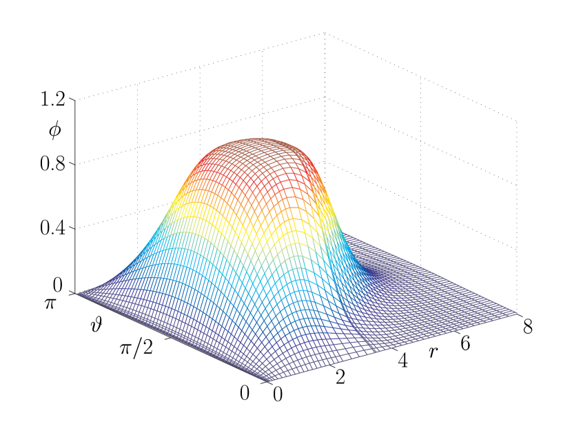
Figure 7: $\phi(r,\vartheta)$ for $N=1$, $P=1$.

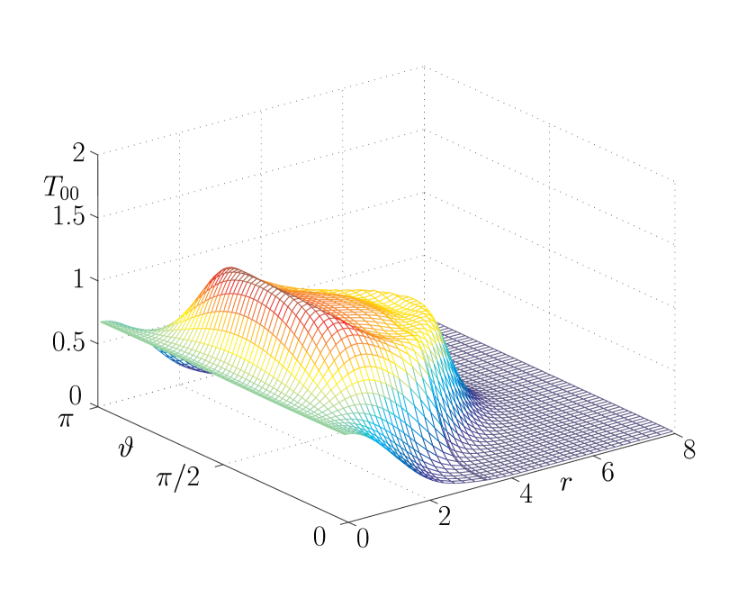
Figure 8: $T_{00}$ for $N=1$, $P=1$.

As one can see from these plots, the distribution of the energy density $T_{00}$ is strongly non-spherical. It has the structure of a deformed ellipsoid for $P=1$, and that of dumbbells oriented along the rotation axis for $P=-1$; in the latter case the energy density vanishes in the equatorial plane. The energies of the first three rotational excitations of the fundamental Q-ball are given in Table 2.

Table 2: Parameters of the rotating solutions with $Q=410$.

$N^{P}$	$l_{\max}$	$E$	$\omega$
$0$	0	307.29	0.76099
$1^{+}$	9	378.36	0.86017
$1^{-}$	8	442.24	0.99164
$2^{+}$	10	433.94	0.96258
$2^{-}$	9	505.66	1.13284
$3^{+}$	9	473.59	1.05277
$3^{-}$	12	528.30	1.31037

As one can see, the energy of the first excitation exceeds the ground state energy by about $20\%$, the next excitation lying again about $20\%$ above. This is in agreement with the expected properties of spinning excitations of a single soliton. In summary, spinning Q-balls comprise a two-parameter family labeled by the values of $(Q,N)$. We have also found evidence for the existence of spinning radial excitations with $n>0$. However, the construction of such solutions is somewhat more involved and we refrain from presenting them in this paper.

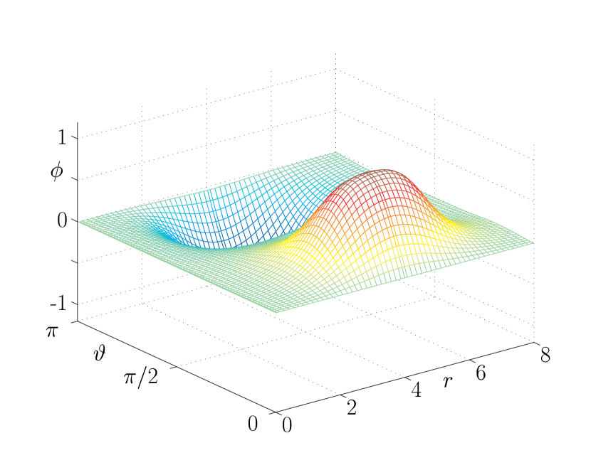
Figure 9: $\phi(r,\vartheta)$ for the $N=1$, $P=-1$.

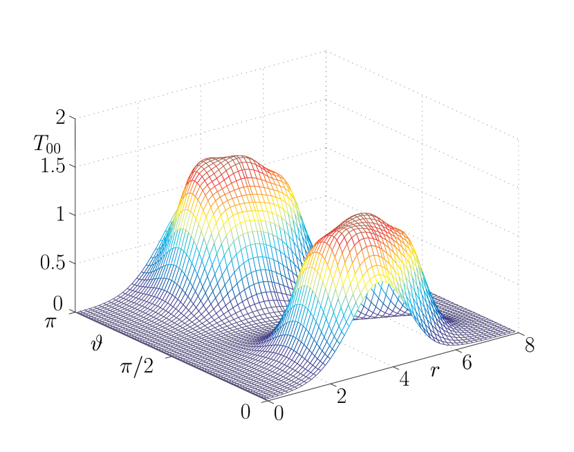
Figure 10: $T_{00}$ for the $N=1$, $P=-1$.

VI Conclusions

The aim of this paper was to find an example of spinning solitons in Minkowski space. We have considered the model of a complex scalar field with a non-renormalizable self-interaction. In the spherically symmetric sector this model contains non-topological solitons, the Q-balls. In addition, we have found an infinite discrete family of radial Q-ball excitations, parameterized by the number of nodes $n$ of the radial field amplitude. Such excited solutions have not been reported in the literature before.

In a second step we have analyzed cylindrically symmetric solutions with explicit harmonic dependence on the azimuthal angle, $\exp(iN\varphi)$, which we call spinning Q-vortices. For such solutions there is a non-zero component of the angular momentum along the $z$-axis, $J=NQ$, where $Q$ is the charge per unit vortex length. In addition, these solutions exhibit radial excitations parameterized by an integer $n$. As a result, such spinning solutions comprise a three-parameter family labeled by $(Q,N,n)$.

Finally, we have considered the full $3+1$ dimensional problem. We have used a version of the spectral method by expanding the field with respect to the complete set of associated Legendre functions. We reduced the PDE to an infinite system of radial ODEs, and then truncating this system at finite order. The parameters of the solutions for the truncated system converge rapidly to some limiting values as the truncation parameter grows. By keeping the charge $Q$ fixed, we have obtained the lowest rotational excitations of the fundamental Q-ball solutions. The angular momentum of these solutions is quantized, $J=NQ$, the energy increases (but not very rapidly) with the angular momentum. As a result, these solutions can be viewed as describing spinning excitations in the one-soliton sector rather than orbital motion in a many-soliton system. To our knowledge, these spinning Q-balls provide the first explicit example of spinning solitons in Minkowski space in $3+1$ dimensions.

- (1) G.S. Adkins, C.R. Nappi and E. Witten, Static properties of nucleons in the Skyrme model, Nucl. Phys. B 228, 552 (1983).
- (2) R. Bartnik and J. McKinnon, Particle-like solutions of the Einstein-Yang-Mills equations, Phys. Rev. Lett. 61, 141 (1988).
- (3) R. Battye and P. Sutcliffe, Q-Ball dynamics, Nucl. Phys. B 590, 329 (2000).
- (4) O. Brodbeck, M. Heusler, N. Straumann and M. S. Volkov, Rotating solitons and non-rotating, non-static black holes, Phys. Rev. Lett. 79, 4310 (1997).
- (5) S.R. Coleman, Q-Balls, Nucl. Phys. B 262, 263 (1985).
- (6) R.L. Davis, Semitopological solitons, Phys. Rev. D 38, 3722 (1988).
- (7) R.L. Davis and E.P.S. Shellard, Cosmic vortons, Nucl. Phys. B 323, 209 (1989).
- (8) H.J. de Vega and F.A. Schaposnik, Electrically charged vortices in non-Abelian gauge theories with Chern-Simons term, Phys. Rev. Lett. 56, 2564 (1986).
- (9) J. Gladikowski and M. Hellmund, Static solitons with non-zero Hopf number, Phys. Rev. D 56, 5194 (1997).
- (10) T. Gisiger and M.B. Paranjape, Solitons in a baby-Skyrme model with invariance under volume/area preserving diffeomorphisms, Phys. Rev. D 55, 7731 (1997).
- (11) M. Heusler, N. Straumann and M.S. Volkov, On rotational excitations and axial deformations of BPS monopoles and Julia-Zee dyons, Phys. Rev. D 58, 105021 (1998).
- (12) R. Jackiw and E.J. Weinberg, Selfdual Chern-Simons solitons, Phys. Rev. Lett. 64, 2234 (1990).
- (13) C. Kim, S. Kim and Y. Kim, Global nontopological vortices, Phys. Rev. D 47, 5434 (1993).
- (14) B. Kleihaus and J. Kunz, A monopole-antimonopole solution of the SU(2) Yang-Mills-Higgs model, Phys. Rev. D 61, 025003 (2000).
- (15) B. Kleihaus, J. Kunz and N. Francisco, Rotating Einstein-Yang-Mills black holes, http://arXiv.org/abs/gr-qc/0207042.
- (16) A. Kusenko, Solitons in the supersymmetric extensions of the standard model, Phys. Lett. B 405, 108 (1997).
- (17) A. Kusenko and M. Shaposhnikov, Supersymmetric Q-Balls as dark matter, Phys. Lett. B 418, 46 (1998).
- (18) T.D. Lee and Y. Pang, Nontopological solitons, Phys. Rept. 221, 251 (1992).
- (19) D. Maison, Uniqueness of the Prasad-Sommerfield monopole solution, Nucl. Phys. B 182, 144 (1981).
- (20) G. Neugebauer and R. Meinel, General relativistic gravitational field of a rigidly rotating disk of dust: Solution in terms of ultraelliptic functions, Phys. Rev. Lett. 75, 3046 (1995).
- (21) B.M.A.G. Piette, B.J. Schroers and W. Zakrzewski, Dynamics of baby skyrmions, Nucl. Phys. B 439, 205 (1995).
- (22) F.E. Schunck and E.W. Mielke, Rotating boson stars, in: Relativity and Scientific Computing, edited by F.W. Hehl, R.A. Puntigam and H. Ruder, Springer (1996) 138–151.
- (23) C.H. Taubes, The existence of a nonminimal solution to the SU(2) Yang-Mills Higgs equations on . Part I, Commun. Math. Phys. 86, 257 (1982).
- (24) C.H. Taubes, The existence of a nonminimal solution to the SU(2) Yang-Mills Higgs equations on . Part II, Commun. Math. Phys. 86, 299 (1982).
- (25) J.J. Van der Bij and E. Radu, On rotating regular non-Abelian solutions, Int. J. Mod. Phys. A 17, 1477 (2002).
- (26) S. Yoshida and Y. Eriguchi, Rotating boson stars in general relativity, Phys. Rev. D 56, 762 (1997).