On a core instability of ’t Hooft Polyakov monopoles

Abstract

We discuss a core instability of ’t Hooft Polyakov monopoles in Alice electrodynamics type of models in which charge conjugation symmetry is gauged. The monopole may deform into a toroidal defect which carries an Alice flux and a (non-localizable) magnetic Cheshire charge.

1 Introduction

Since the pioneering work of ’t Hooft and Polyakov [1] magnetic monopoles have been studied in detail in many different models. In this paper we address the question of stability of the core of the fundamental, spherically symmetric, monopole configuration, a stability which appears to be so obvious that it was never seriously questioned. We will show that in a rather simple model the spherically symmetric unit charge magnetic monopole is not the global minimal energy solution for all parameter values in the model. The fact that the core topology is not uniquely determined by the boundary conditions and different core topologies can be deformed into each other was already established earlier [2]. As we will indicate, Alice theories have a special feature which makes it more plausible that such a core deformation really may be favored energetically. Our interest in this problem was rekindled by some observations that were made in theories with global symmetries [3].

We start by briefly summarizing the main features of Alice Electrodynamics (AED), then we discuss the particular tensor model we will use to explicitly establish the core instability and determine some region in parameter space where this occurs.

2 A core deformation in Alice Electrodynamics

Alice electrodynamics (AED) is a gauge theory with gauge group $H=U(1)\ltimes\mathbb{Z}_{2}\sim O(2)$, i.e. a minimally non-abelian extension of ordinary electrodynamics. The nontrivial $\mathbb{Z}_{2}$ transformation reverses the direction of the electric and magnetic fields and the sign of the charges. In other words, in Alice electrodynamics charge conjugation symmetry is gauged. However, as this non-abelian extension is discrete, it only affects electrodynamics through certain global (topological) features, such as the appearance of Alice fluxes and Cheshire charges [4, 5]. The possibility of a non-localizable magnetic Cheshire charge will be of great importance in our study of the core instability of the monopole. The topological structure of $U(1)\ltimes\mathbb{Z}_{2}$ differs from that of $U(1)$ in a few subtle points. AED allows topologically stable localized fluxes since $\Pi_{0}(U(1)\ltimes\mathbb{Z}_{2})=\mathbb{Z}_{2}$, the so called Alice fluxes. Note that in this theory this flux is coëxisting with the unbroken $U(1)$ of electromagnetism and is therefore not an ordinary “magnetic” flux. Just as a $U(1)$ gauge theory, AED may contain magnetic monopoles, which follows from the fact that $\Pi_{1}(U(1)\ltimes\mathbb{Z}_{2})=\mathbb{Z}$. We note however, that due to the fact that the $\mathbb{Z}_{2}$ and the $U(1)$ part of the gauge group do not commute, magnetic charges of opposite sign belong to the same topological sector. Alice phases can be generated by spontaneously breaking $SU(2)$ (or $SO(3)$) to $U(1)\ltimes\mathbb{Z}_{2}$, for example by choosing a Higgs field in a 5-dimensional representation of the gauge group. In that case the topological defects, fluxes [6, 7] and monopoles [1], will correspond to regular classical solutions. It was pointed out long ago that there are interesting issues concerning the core stability of magnetic monopoles. Fixing the asymptotics of the Higgs field, the core (i.e. the zeros of the Higgs field) may have different topologies, notably that of a ring rather than the conventional point. These core topologies can be smoothly deformed into each other and it is a question of energetics what will be the lowest energy monopole state [2]. We return to this issue in this paper because the core deformation would be accompanied by the rather unusual delocalized version of (magnetic) charge, the so called Cheshire charge. In the specific AED model we studied the Higgs field is a symmetric tensor, whose vacuum expectation value may be depicted as a bidirectional arrow. The head-tail symmetry of the order parameter reflects the charge conjugation symmetry of the theory. In AED the spherical monopole can be punctured and be deformed into an Alice loop, this configuration is consistent with the order parameter because of the the head-tail symmetry of the order parameter. In figure 1 we show a slice of this core deformation. Note that the order parameter on the right hand side of figure 1 only rotates over an angle $\pi$ when going around a single flux. This is the hallmark for an Alice flux, i.e. the core deformed spherical monopole is in fact an Alice loop carrying a magnetic Cheshire charge.

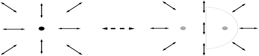
Figure 1: A slice of the core deformation of the spherical monopole into an Alice loop, carrying a magnetic Cheshire charge.

3 The tensor model of AED

To be able to answer stability questions of the spherically symmetric monopole configuration (or the Cheshire charged Alice loop) we consider an explicit model. In the remainder we focus on the original tensor Alice model [8]. The action of this model is given by:

$$S=\int d^{4}x\ \{\frac{1}{4}F^{a,\mu\nu}F^{a}_{\mu\nu}+\frac{1}{4}Tr(D^{\mu}\Phi D_{\mu}\Phi)-V(\Phi)\},$$ (1)

where the Higgs field $\Phi=\Phi^{ab}$ is a real, symmetric, traceless $3\times 3$ matrix, i.e. $\Phi$ is in the five dimensional representation of $SO(3)$ and $D_{\mu}\Phi=\partial_{\mu}\Phi-ie[A_{\mu},\Phi]$, with $A_{\mu}=A^{a}_{\mu}T_{a}$, where $T_{a}$ are the generators of $SO(3)$. The most general renormalizeable potential is given by [9]:

$$V=-\frac{1}{2}\mu^{2}Tr\Phi^{2}-\frac{1}{3}\gamma Tr\Phi^{3}+\frac{1}{4}\lambda(Tr\Phi^{2})^{2}$$ (2)

with $\gamma>0$, since $(\Phi,\gamma)=(-\Phi,-\gamma)$.
For a suitable range of the parameters in the potential, the gauge symmetry of the model will be broken to the symmetry of AED. In the “unitary” gauge, where the Higgs field is diagonal, the ground state is (up to permutations) given by the following matrix:

$$\Phi_{0}=\left(\begin{array}[]{ccc}-f&0&0\\ 0&-f&0\\ 0&0&2f\end{array}\right)$$ (3)

with $f=\frac{\gamma}{12\lambda}(1+\sqrt{1+\frac{24\mu^{2}\lambda}{\gamma^{2}}})$. The full action has four parameters, $e,\mu^{2},\gamma,\lambda$, this number can be reduced to two dimensionless parameters by appropriate rescalings of the variables. A physical choice for these dimensionless parameters is to take the ratio’s of the masses that one finds from perturbing around the homogeneous minimum. To determine these, we write the action in the unitary gauge where the massless components of $\Phi$ have been absorbed by the gauge fields. The physical components of the Higgs field may be expanded as:

$$\Phi(x^{\mu})=\Phi_{0}+\sqrt{2}\phi_{1}(x^{\mu})E_{1}+\sqrt{2}\phi_{2}(x^{\mu})~{}R_{3}(a(x^{\mu}))E_{2}R_{3}(a(x^{\mu}))^{T}$$ (4)

with:

$$E_{1}=\frac{1}{\sqrt{6}}\left(\begin{array}[]{ccc}-1&0&0\\ 0&-1&0\\ 0&0&2\end{array}\right)~{};~{}~{}E_{2}=\frac{1}{\sqrt{2}}\left(\begin{array}[]{ccc}1&0&0\\ 0&-1&0\\ 0&0&0\end{array}\right)~{};~{}~{}E_{3}=\frac{1}{\sqrt{2}}\left(\begin{array}[]{ccc}0&0&1\\ 0&0&0\\ 1&0&0\end{array}\right)$$ (5)

and $R_{i}$ are the usual rotation matrices. To second order, the potential $V(\Phi)$ takes the following form:

$$V(\Phi)=const.+(2\mu^{2}+\gamma f)\phi_{1}^{2}+3\gamma f|\phi_{2}|^{2}+...$$ (6)

yielding the two distinct masses of the Higgs modes. Next we look at the ’kinetic’ term, $\frac{1}{4}Tr(D^{\mu}\Phi D_{\mu}\Phi)$, of the Higgs field. Inserting the previous expressions for the Higgs field, we find:

$$\frac{1}{4}Tr(D^{\mu}\Phi D_{\mu}\Phi)=\frac{1}{2}(\partial_{\mu}\phi_{1})^{2}+\frac{1}{2}|D_{\mu}^{3}\phi_{2}|^{2}+\frac{9}{2}e^{2}f^{2}[(A_{\mu}^{1})^{2}+(A_{\mu}^{2})^{2}]+...$$ (7)

with: $D_{\mu}^{3}=\partial_{\mu}-i2eA^{3}_{\mu}$. The second term shows that the $\phi_{2}$ component of the Higgs field carries a charge $2e$ with respect to the unbroken $U(1)$ component $A_{\mu}^{3}$ of the gauge field. The first term describes the usual charge neutral Higgs particle and the third term yields the mass of the charged gauge fields. Thus the relevant lowest order action is given by:

$$S=\int d^{4}x\{\frac{1}{4}F_{\mu\nu}^{a}F^{a,\mu\nu}+\frac{1}{2}(\partial_{\mu}\phi_{1})^{2}+\frac{1}{2}|D_{\mu}^{3}\phi_{2}|^{2}-\frac{1}{2}m_{1}^{2}\phi_{1}^{2}$$ (8)

$$-\frac{1}{2}m_{2}^{2}|\phi_{2}|^{2}-\frac{1}{2}m_{A}^{2}[(A_{\mu}^{1})^{2}+(A_{\mu}^{2})^{2}]+...\}$$

with $m_{1}^{2}=4\mu^{2}+2\gamma f$, $m_{2}^{2}=6\gamma f$ and $m_{A}^{2}=9e^{2}f^{2}$. Thus two degrees of freedom of the five dimensional Higgs field are ’eaten’ by the broken gauge fields, one degree of freedom forms the real neutral scalar field and two degrees of freedom form the complex (doubly charged) scalar field. To specify a point in the parameter space of classical solutions we may, up to irrelevant rescalings, use the dimensionless mass ratio’s $\frac{m_{1}}{m_{2}}$ and $\frac{m_{A}}{m_{2}}$.

4 The core instability

In this section we will show that the monopole core, see figure 2, becomes meta- or unstable for a certain range in the parameter space of the theory. Our strategy is as follows. Using numerical methods, we look for the global and local minima of the monopole energy within a class of configurations given by a suitable ansatz. We restrict ourselves to static configurations and the ansatz we use contains the spherically symmetric ’t Hooft-Polyakov monopole configuration as a special case [8]. The ansatz is cylindrically symmetric and also has reflection symmetry with respect to the $z=0$ plane.

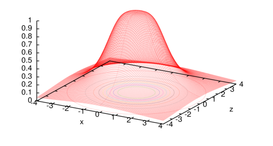
Figure 2: A slice of a magnetic monopole solution at $y=0$, we plotted $1-\frac{Tr\Phi^{2}}{f^{2}}$.
      $\frac{m_{1}}{m_{2}}=0.571$ and $\frac{m_{A}}{m_{2}}=0.0095$.

The ansatz for the Higgs field is:

$$\Phi(z,\rho,\theta=0)=\phi_{1}(z,\rho)E_{1}+\phi_{2}(z,\rho)E_{2}+\phi_{3}(z,\rho)E_{3}$$ (9)

and

$$\Phi(z,\rho,\theta)=R_{3}(\theta)\Phi(z,\rho,\theta=0)R_{3}(\theta)^{T}$$ (10)

The ansatz for the gauge fields is simply given by $eA_{i}^{j}=-\epsilon_{ijk}\frac{x^{k}}{x^{2}}A(z,\rho)$, very similar to the one for the spherically symmetric monopole [1], except that we allow $A(z,\rho)$ to depend on $\rho$ and $z$ instead of only depending on $r=\sqrt{\rho^{2}+z^{2}}$. The boundary conditions for $r\to\infty$ are the boundary conditions of the spherically symmetric monopole as in [8], i.e. $A(z,\rho)$ goes to one and the Higgs field to $\Phi(z,\rho,\theta)=R_{3}(\theta)R_{2}(\arccos(\frac{z}{r}))\Phi_{0}R_{2}(\arccos(\frac{z}{r}))^{T}R_{3}(\theta)^{T}$.
The boundary conditions for $\rho=0$ and $z=0$ follow by imposing the cylindrical and reflection symmetry and are given in the table below:

$$\begin{array}[]{|c||c|c|}\hline\cr&\rho=0&z=0\\ \hline\cr\phi_{1}&\partial_{\rho}\phi_{1}=0&\partial_{z}\phi_{1}=0\\ \phi_{2}&\partial_{\rho}\phi_{2}=\phi_{2}=0&\partial_{z}\phi_{2}=0\\ \phi_{3}&\phi_{3}=0&\phi_{3}=0\\ A&\partial_{\rho}A=0&\partial_{z}A=0\\ \hline\cr\end{array}$$

It is easy to see that these boundary conditions are also met by the spherically symmetric monopole ansatz, so it is indeed contained in our more general ansatz. The important point is that our ansatz in principle allows for the possibility of an Alice loop configuration carrying a magnetic Cheshire charge, see figure 3. These are exactly the two configurations that we want to compare.

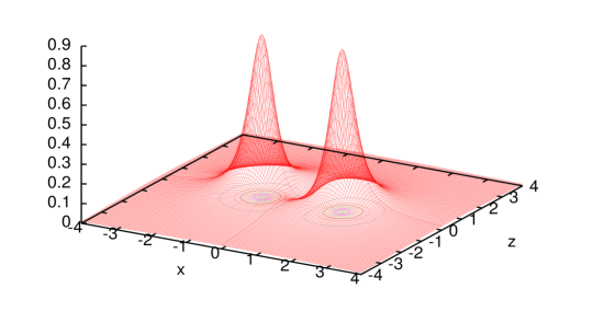
Figure 3: A slice of a Cheshire charged Alice loop configuration at $y=0$, we plotted $1-\frac{Tr\Phi^{2}}{f^{2}}$.
       $\frac{m_{1}}{m_{2}}=0.882$ and $\frac{m_{A}}{m_{2}}=0.0073$.

Using the ansatz, we indeed found configurations having less energy than the spherically symmetric monopole solution, at least in a certain region of the parameter space. We even found that the spherically symmetric monopole is not always locally stable. Strictly speaking our non spherical symmetric configurations, the magnetically Cheshire charged configurations, are only approximate solutions and consequently, they only yield an upper bound to the energy of the true solution. Obviously this suffices to show the instability of the standard monopole and we do expect that the true solution is very close to this magnetically Cheshire charged Alice loop configuration. In this paper we only present the results concerning configurations along a specific path in the parameter space of the theory. We refer to an forthcoming paper [10] where we will determine the stability, meta stability and instability regions of both configurations, within this ansatz for the ’full’ parameter space of the model. The path, see figure 4, we have considered covers three regions of the model. In one region, on the left of point A, the monopole is the only stable solution. In the next region, between point A and C, both the monopole and the Alice loop are locally stable and in the last, on the right of point C, the Alice loop is the only locally stable configuration. Somewhere half way the middle region, point B, the monopole is no longer the global minimum, whereas the Alice loop is, i.e. the monopole is only a meta stable solution.

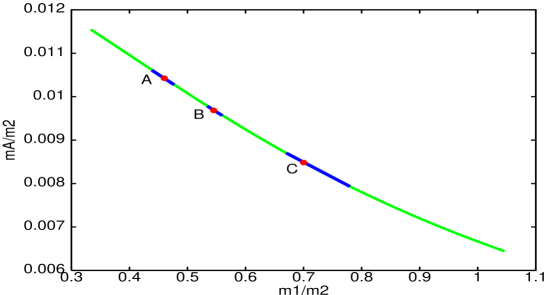
Figure 4: Going from the left to the right: After point A, the thick line represents the errorbar along the path, the Alice loop becomes locally stable, between point A and C both the monopole and the Alice loop are locally stable. After point B the monopole is only meta stable and after point C it is even an unstable solution.

The two extreme sides of the path can be understood as follows. The two masses $m_{1}$ and $m_{2}$ correspond to the energy cost to deviate from the vacuum in two different ways. $m_{1}$ is the energy cost for deviating in the neutral direction or ’length’ of the Higgs field, while $m_{2}$ is the energy cost in deviating in a non uniaxial direction. Thus in the limit $\frac{m_{1}}{m_{2}}\to 0$, the deviations in the non uniaxial directions are suppressed. There one would expect the uniaxial monopole to be the global stable solution. In the opposite limit, $\frac{m_{1}}{m_{2}}\to\infty$, one would expect an ’escape’ into the non-uniaxial directions and a suppression in the length deviation, signaling the meta stability of the uniaxial monopole, as is the case for the Alice loop configuration. Notice that the length of the Higgs field never becomes zero in the case of the Alice loop, i.e. $1-\frac{Tr\Phi^{2}}{f^{2}}$ never becomes one in figure 3.

5 Conclusion and outlook

In this letter we showed that monopoles of the ’t Hooft Polyakov type may exhibit a core instability, depending on the parameters of the theory. In one part of the parameter space, the spherical monopole is the global minimum. In another part it corresponds to a local minimum and there even is a region where it is unstable. We found that the competing configuration is a magnetically Cheshire charged Alice loop. Since we worked within a limited ansatz, the regions we found for the monopole global and/or local stability are in fact only upper bounds on the stability regions of the spherical monopole, and these regions can only become smaller when no (or less) restrictions are put on the configurations one may sample. At the moment we are scanning the ’full’ parameter space of the model. The results obtained as well as more detailed information on the model, the simulations and the configurations we found, will be published elsewhere [10].

References

- [1] G. ’t Hooft. Magnetic monopoles in unified gauge theories. Nucl. Phys., B79:276–284, 1974; A. M. Polyakov. Particle spectrum in quantum field theory. JETP Lett., 20:194–195, 1974.
- [2] F. Alexander Bais and Per John. Core deformations of topological defects. Int. J. Mod. Phys., A10:3241–3258, 1995.
- [3] R.Rosso and E.G.Virga. Metastable nematic hedgehogs. J.Phys.A, 29:4247–4264, 1996; S.Kralj and E.G.Virga. Universal fine structure of nematic hedgehogs. J.Phys.A, 34:829–838, 2001; S.Mkaddem and Jr. E.C.Gartland. Fine struture of defects in radial nematic droplets. Phys. Rev. E, 62:6694–6705, 2000.
- [4] A. S. Schwarz. Field theories with no local conservation of the electric charge. Nucl. Phys., B 208:141, 1982.
- [5] Mark Alford, Katherine Benson, Sidney Coleman, John March-Russell, and Frank Wilczek. Zero modes of nonabelian vortices. Nucl. Phys., B 349:414–438, 1991.
- [6] H. B. Nielsen and P. Olesen. Vortex line models for dual strings. Nucl. Phys., B 61:45–61, 1973.
- [7] J. Striet and F. A. Bais. Simple models with alice fluxes. Phys. Lett., B497:172–180, 2000.
- [8] R. Shankar. More so(3) monopoles. Phys. Rev., D 14:1107, 1976.
- [9] Howard Georgi and Sheldon L. Glashow. Spontaneously broken gauge symmetry and elemenatry particle masses. Phys. Rev., D 6:2977–2982, 1972.
- [10] F. A. Bais and J. Striet. in preparation.