Symmetries of Toric Duality

Abstract:

This paper serves to elucidate the nature of toric duality dubbed in hep-th/0003085 in the construction for world volume theories of D-branes probing arbitrary toric singularities. This duality will be seen to be due to certain permutation symmetries of multiplicities in the gauged linear sigma model fields. To this symmetry we shall refer as “multiplicity symmetry.” We present beautiful combinatorial properties of these multiplicities and rederive all known cases of torically dual theories under this new light. We also initiate an understanding of why such multiplicity symmetry naturally leads to monodromy and Seiberg duality. Furthermore we discuss certain “flavor” and “node” symmetries of the quiver and superpotential and how they are intimately related to the isometry of the background geometry, as well as how in certain cases complicated superpotentials can be derived by observations of the symmetries alone.

1 Introduction

The study of string theory on various back-grounds, in particular space-time singularities, is by now an extensively investigated matter. Of special interest are algebraic singularities which locally model Calabi-Yau threefolds so as to produce, on the world-volume of D-branes transversely probing the singularity, classes of supersymmetric gauge theories.

Using the techniques of the gauged linear sigma model [1] as a symplectic quotienting mechanism, toric geometry has been widely used [2, 3, 4, 5] to analyse the D-brane theories probing toric singularities. The singularity resolution methods fruitfully developed in the mathematics of toric geometry have been amply utilised in understanding the world-volume gauge theory, notably its IR moduli space, which precisely realises the singularity being probed.

To deal with the problem of finding the gauge theory on the D-brane given an arbitrary toric singularity which it probes, a unified algorithmic outlook to the existing technology [2, 3, 4, 5] of partial resolution of Abelian orbifolds has been established [6]. One interesting byproduct of the algorithm is the harnessing of its non-uniqueness to explicitly construct various theories with vastly different matter content and superpotential which flow in the IR to the same moduli space parametrised by the toric variety [6, 7]. In fact these theories are expected [8, 9] to be completely dual in the IR as field theories. The identification of the moduli space is but one manifestation, in addition, they should have the same operator spectrum, same relevant and marginal deformations and correlation functions. The phenomenon was dubbed toric duality.

Recently this duality has caught some attention [8, 9, 12, 13], wherein three contrasting perspectives, respectively brane-diamond setups, dual variables in field theory as well as ${\cal N}=1$ geometric transitions, have lead to the same conjecture that Toric Duality is Seiberg Duality for ${\cal N}=1$ theories with toric moduli spaces. In addition, the same phases have been independently arrived at via $(p,q)$-web configurations [15].

The Inverse Algorithm of [6] remains an effective - in the sense of reducing the computations to nothing but linear algebra and integer programming - method of deriving toric (and hence Seiberg) dual theories. With this convenience is a certain loss of physical and geometrical intuition: what indeed is happening to the fields (both in the sigma model and in the brane world-volume theory) as one proceed with the linear transformations? Moreover, in the case of the cone over the third del Pezzo surface (dP3), various phases have been obtained using independent methods [8, 9, 13] while they have so far not been attained by the Inverse Algorithm.

The purpose of this writing is clear. We first supplant the present shortcoming by explicitly obtaining all phases of dP3. In due course we shall see the true nature of toric duality: that the unimodular degree of freedom whence it arises as claimed in [7] - though such unimodularity persists as a symmetry of the theory - is but a special case. It appears that the quintessence of toric duality, with regard to the Inverse Algorithm, is certain multiplicity of fields in the gauged linear sigma model. Permutation symmetry within such multiplicities leads to torically dual theories. Furthermore we shall see that these multiplicities have beautiful combinatorial properties which still remain largely mysterious.

Moreover, we also discuss how symmetries of the physics, manifested through “flavor symmetries” of multiplets of bi-fundamentals between two gauge factors, and through “node symmetries” of the permutation automorphism of the quiver diagram. We shall learn how in many cases the isometry of the singularity leads us to such symmetries of the quiver. More importantly, we shall utilise such symmetries to determine, very often uniquely, the form of the superpotential.

The outline of the paper is as follows. In Section 2 we present the multiplicities of the GLSM fields for the theories $\hbox{$\,\vrule height=6.45831pt,width=0.4pt,depth=0.0pt\kern-3.00003pt{\rm C}$}^{2}/\mathchoice{\hbox{\cmss Z\kern-3.99994ptZ}}{\hbox{\cmss Z\kern-3.99994ptZ}}{\lower 0.9pt\hbox{\cmsss Z\kern-2.79996ptZ}}{\lower 1.2pt\hbox{\cmsss Z\kern-2.79996ptZ}}_{n}$ as well as some first cases of $\hbox{$\,\vrule height=6.45831pt,width=0.4pt,depth=0.0pt\kern-3.00003pt{\rm C}$}^{3}/(\mathchoice{\hbox{\cmss Z\kern-3.99994ptZ}}{\hbox{\cmss Z\kern-3.99994ptZ}}{\lower 0.9pt\hbox{\cmsss Z\kern-2.79996ptZ}}{\lower 1.2pt\hbox{\cmsss Z\kern-2.79996ptZ}}_{k}\times\mathchoice{\hbox{\cmss Z\kern-3.99994ptZ}}{\hbox{\cmss Z\kern-3.99994ptZ}}{\lower 0.9pt\hbox{\cmsss Z\kern-2.79996ptZ}}{\lower 1.2pt\hbox{\cmsss Z\kern-2.79996ptZ}}_{m})$ and observe beautiful combinatorial properties thereof. In Section 3 we show how toric duality really originates from permutation symmetries from the multiplicities and show how the phases of known torically dual theories can be obtained in this new light. Section 4 is devoted to the analysis of node and flavor symmetries. It addresses the interesting problem of how one may in many cases obtain the complicated forms of the superpotential by merely observing these symmetries. Then in Section 5 we briefly give an argument why toric duality should stem from such multiplicities in the GLSM fields in terms of monodromy actions on homogeneous cöordinates. We conclude and give future prospects in Section 6.

2 Multiplicities in the GLSM Fields

We first remind the reader of the origin of the multiplicity in the homogeneous coordinates of the toric variety as described by Witten’s gauged linear sigma model (GLSM) language [1]. The techniques of [2, 3, 4, 5] allow us to write the D-flatness and F-flatness conditions of the world-volume gauge theory on an equal footing.

At the end of the day, the $U(1)^{n}$ ${\cal N}=1$ theory with $m$ bi-fundamentals on the D-brane is described by $c$ fields $p_{i}$ subject to $c-3$ moment maps: this gives us the $(c-3)\times c$ charge matrix $Q_{t}$. The integral cokernel of $Q_{t}$ is a $3\times c$ matrix $G_{t}$; its columns, up to repetition, are the nodes of the three-dimensional toric diagram corresponding to the IR moduli space of the theory. These $c$ fields $p_{i}$ are the GLSM fields of [1], or in the mathematics literature, the so-called homogeneous coordinates of the toric variety [17]. The details of this forward algorithm from gauge theory data to toric data have been extensively presented as a flow-chart in [6, 7] and shall not be belaboured here again.

The key number to our analyses shall be the integer $c$. It is so that the $(r+2)\times c$ matrix $T$ describes the integer cone dual to the $(r+2)\times m$ matrix $K$ coming from the F-terms. As finding dual cones (and indeed Hilbert bases of integer polytopes) is purely an algorithmic method, there is in the literature so far no known analytic expression for $c$ in terms of $m$ and $r$; overcoming this deficiency would be greatly appreciated.

A few examples shall serve to illustrate some intriguing combinatorial properties of this multiplicity.

We begin with the simple orbifold $\hbox{$\,\vrule height=6.45831pt,width=0.4pt,depth=0.0pt\kern-3.00003pt{\rm C}$}^{3}/\mathchoice{\hbox{\cmss Z\kern-3.99994ptZ}}{\hbox{\cmss Z\kern-3.99994ptZ}}{\lower 0.9pt\hbox{\cmsss Z\kern-2.79996ptZ}}{\lower 1.2pt\hbox{\cmsss Z\kern-2.79996ptZ}}_{n}$ with the $\mathchoice{\hbox{\cmss Z\kern-3.99994ptZ}}{\hbox{\cmss Z\kern-3.99994ptZ}}{\lower 0.9pt\hbox{\cmsss Z\kern-2.79996ptZ}}{\lower 1.2pt\hbox{\cmsss Z\kern-2.79996ptZ}}_{n}$ action on the coordinates $(x,y,z)$ of $\hbox{$\,\vrule height=6.45831pt,width=0.4pt,depth=0.0pt\kern-3.00003pt{\rm C}$}^{3}$ as $(x,y,z)\rightarrow(\omega^{a}x,\omega^{b}y,\omega^{-1}z)$ such that $\omega$ is the $n$th root of unity and $a+b-1\equiv 0(\bmod n)$ to guarantee that $Z_{n}\subset SU(3)$ so as to ensure that the resolution is a Calabi-Yau threefold. This convention in chosen in accordance with the standard literature [2, 3, 4, 5].

Let us first choose $a=0$ so that the singularity is effectively $\hbox{$\,\vrule height=6.45831pt,width=0.4pt,depth=0.0pt\kern-3.00003pt{\rm C}$}\times\hbox{$\,\vrule height=6.45831pt,width=0.4pt,depth=0.0pt\kern-3.00003pt{\rm C}$}^{2}/\mathchoice{\hbox{\cmss Z\kern-3.99994ptZ}}{\hbox{\cmss Z\kern-3.99994ptZ}}{\lower 0.9pt\hbox{\cmsss Z\kern-2.79996ptZ}}{\lower 1.2pt\hbox{\cmsss Z\kern-2.79996ptZ}}_{n}$; with the toric diagram of the Abelian ALE piece we are indeed familiar: the fan consists of a single 2-dimensional cone generated by $e_{2}$ and $ne_{1}-e_{2}$ [16]. This well-known ${\cal N}=2$ theory, under such embedding as a $\hbox{$\,\vrule height=6.45831pt,width=0.4pt,depth=0.0pt\kern-3.00003pt{\rm C}$}^{3}$ quotient, can thus be cast into ${\cal N}=1$ language. Applying the Forward Algorithm of [2, 3, 4, 5] to the ${\cal N=}1$ SUSY gauge theory on this orbifold should give us none other than the toric diagram for $\hbox{$\,\vrule height=6.45831pt,width=0.4pt,depth=0.0pt\kern-3.00003pt{\rm C}$}^{2}/\mathchoice{\hbox{\cmss Z\kern-3.99994ptZ}}{\hbox{\cmss Z\kern-3.99994ptZ}}{\lower 0.9pt\hbox{\cmsss Z\kern-2.79996ptZ}}{\lower 1.2pt\hbox{\cmsss Z\kern-2.79996ptZ}}_{n}$. This is indeed so as shown in the following table. What we are interested in is the matrix $G_{t}$, whose integer nullspace is the charge matrix $Q_{t}$ of the linear sigma model fields. We should pay special attention to the repetitions in the columns of $G_{t}$.

2.1 $\hbox{$\,\vrule height=6.45831pt,width=0.4pt,depth=0.0pt\kern-3.00003pt{\rm C}$}^{2}/\mathchoice{\hbox{\cmss Z\kern-3.99994ptZ}}{\hbox{\cmss Z\kern-3.99994ptZ}}{\lower 0.9pt\hbox{\cmsss Z\kern-2.79996ptZ}}{\lower 1.2pt\hbox{\cmsss Z\kern-2.79996ptZ}}_{n}$

We present the matrix $G_{t}$, whose columns, up to multiplicity, are the nodes of the toric diagram for $\hbox{$\,\vrule height=6.45831pt,width=0.4pt,depth=0.0pt\kern-3.00003pt{\rm C}$}^{2}/\mathchoice{\hbox{\cmss Z\kern-3.99994ptZ}}{\hbox{\cmss Z\kern-3.99994ptZ}}{\lower 0.9pt\hbox{\cmsss Z\kern-2.79996ptZ}}{\lower 1.2pt\hbox{\cmsss Z\kern-2.79996ptZ}}_{n}$ for some low values of $n$:

$$\begin{array}[]{|c|l|}\hline\cr n=2&{\scriptsize\left(\matrix{0&0&0&0&1\cr-1&0&0&1&0\cr 2&1&1&0&0\cr}\right)}\\ \hline\cr n=3&{\scriptsize\left(\matrix{0&0&0&0&0&0&0&0&1\cr-2&-1&-1&-1&0&0&0&1&0\cr 3&2&2&2&1&1&1&0&0\cr}\right)}\\ \hline\cr n=4&{\scriptsize\left(\matrix{0&0&0&0&0&0&0&0&0&0&0&0&0&0&0&0&1\cr-3&-2&-2&-2&-2&-1&-1&-1&-1&-1&-1&0&0&0&0&1&0\cr 4&3&3&3&3&2&2&2&2&2&2&1&1&1&1&0&0\cr}\right)}\\ \hline\cr\end{array}$$

We plot in Figure 1 the above vectors in $\mathchoice{\hbox{\cmss Z\kern-3.99994ptZ}}{\hbox{\cmss Z\kern-3.99994ptZ}}{\lower 0.9pt\hbox{\cmsss Z\kern-2.79996ptZ}}{\lower 1.2pt\hbox{\cmsss Z\kern-2.79996ptZ}}^{3}$ and note that they are co-planar, as guaranteed by the Calabi-Yau condition. The black numbers labelling the nodes are the multiplicity of the vectors (in blue) corresponding to the nodes in the toric diagram.

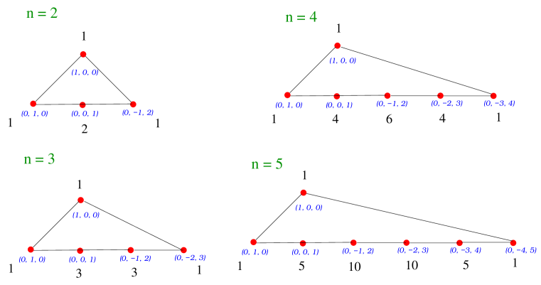
Figure 1: The familiar toric diagrams for $\hbox{$\,\vrule height=6.45831pt,width=0.4pt,depth=0.0pt\kern-3.00003pt{\rm C}$}^{2}/(\mathchoice{\hbox{\cmss Z\kern-3.99994ptZ}}{\hbox{\cmss Z\kern-3.99994ptZ}}{\lower 0.9pt\hbox{\cmsss Z\kern-2.79996ptZ}}{\lower 1.2pt\hbox{\cmsss Z\kern-2.79996ptZ}}_{k}\times\mathchoice{\hbox{\cmss Z\kern-3.99994ptZ}}{\hbox{\cmss Z\kern-3.99994ptZ}}{\lower 0.9pt\hbox{\cmsss Z\kern-2.79996ptZ}}{\lower 1.2pt\hbox{\cmsss Z\kern-2.79996ptZ}}_{m})$, but with the multiplicity of the sigma model fields explicitly labelled.

These toric diagrams in Figure 1 are indeed as expected and are the well-known examples of $\hbox{$\,\vrule height=6.45831pt,width=0.4pt,depth=0.0pt\kern-3.00003pt{\rm C}$}^{2}/\mathchoice{\hbox{\cmss Z\kern-3.99994ptZ}}{\hbox{\cmss Z\kern-3.99994ptZ}}{\lower 0.9pt\hbox{\cmsss Z\kern-2.79996ptZ}}{\lower 1.2pt\hbox{\cmsss Z\kern-2.79996ptZ}}_{n}$. Now note the multiplicities: a pattern in accordance with Pascal’s triangle can clearly be observed. For general $n$, we expect 1’s on the extremal vertices of the triangles while for the $i$th internal colinear node, we have multiplicity ${\scriptsize\left(\matrix{n\cr i}\right)}$. Therefore for this case $c=\sum\limits_{i=1}^{n}{\scriptsize\left(\matrix{n\cr i}\right)}+1=2^{n}+1$. Though we do not have a general proof of this beautiful pattern, we can prove explicitly this expression for $c$, which we leave to the Appendix.

2.2 $\hbox{$\,\vrule height=6.45831pt,width=0.4pt,depth=0.0pt\kern-3.00003pt{\rm C}$}^{3}/(\mathchoice{\hbox{\cmss Z\kern-3.99994ptZ}}{\hbox{\cmss Z\kern-3.99994ptZ}}{\lower 0.9pt\hbox{\cmsss Z\kern-2.79996ptZ}}{\lower 1.2pt\hbox{\cmsss Z\kern-2.79996ptZ}}_{k}\times\mathchoice{\hbox{\cmss Z\kern-3.99994ptZ}}{\hbox{\cmss Z\kern-3.99994ptZ}}{\lower 0.9pt\hbox{\cmsss Z\kern-2.79996ptZ}}{\lower 1.2pt\hbox{\cmsss Z\kern-2.79996ptZ}}_{k})$

As pointed out in [6], in the study of arbitrary toric singularities of local Calabi-Yau threefolds, one must be primarily concerned with the 3-dimensional Abelian quotient $\hbox{$\,\vrule height=6.45831pt,width=0.4pt,depth=0.0pt\kern-3.00003pt{\rm C}$}^{3}/(\mathchoice{\hbox{\cmss Z\kern-3.99994ptZ}}{\hbox{\cmss Z\kern-3.99994ptZ}}{\lower 0.9pt\hbox{\cmsss Z\kern-2.79996ptZ}}{\lower 1.2pt\hbox{\cmsss Z\kern-2.79996ptZ}}_{k}\times\mathchoice{\hbox{\cmss Z\kern-3.99994ptZ}}{\hbox{\cmss Z\kern-3.99994ptZ}}{\lower 0.9pt\hbox{\cmsss Z\kern-2.79996ptZ}}{\lower 1.2pt\hbox{\cmsss Z\kern-2.79996ptZ}}_{k})$. Partial resolutions from the latter using the Inverse Algorithm suffices to handle the world volume gauge theory. Such quotients have also been extensively investigated in [2, 3, 4, 5, 23, 24]

As is well-known, the toric diagrams for these singularities are $(k+1)\times(k+1)$ isosceles triangles. However current restrictions on the running time prohibits constructing the linear sigma model to high values of $k$. We have drawn these diagrams for the first two cases, explicating the multiplicity in Figure 2. From the first two cases we already observe a pattern analogous to the above $\hbox{$\,\vrule height=6.45831pt,width=0.4pt,depth=0.0pt\kern-3.00003pt{\rm C}$}^{2}/\mathchoice{\hbox{\cmss Z\kern-3.99994ptZ}}{\hbox{\cmss Z\kern-3.99994ptZ}}{\lower 0.9pt\hbox{\cmsss Z\kern-2.79996ptZ}}{\lower 1.2pt\hbox{\cmsss Z\kern-2.79996ptZ}}_{n}$ case: each side of the triangle has the multiplicity according to the Pascal’s Triangle. This is to be expected as one can partially resolve the singularity to the $\hbox{$\,\vrule height=6.45831pt,width=0.4pt,depth=0.0pt\kern-3.00003pt{\rm C}$}^{2}$ orbifold. We still do not have a general rule for the multiplicity of the inner point, except in the special case of $\hbox{$\,\vrule height=6.45831pt,width=0.4pt,depth=0.0pt\kern-3.00003pt{\rm C}$}^{3}/(\mathchoice{\hbox{\cmss Z\kern-3.99994ptZ}}{\hbox{\cmss Z\kern-3.99994ptZ}}{\lower 0.9pt\hbox{\cmsss Z\kern-2.79996ptZ}}{\lower 1.2pt\hbox{\cmsss Z\kern-2.79996ptZ}}_{3}\times\mathchoice{\hbox{\cmss Z\kern-3.99994ptZ}}{\hbox{\cmss Z\kern-3.99994ptZ}}{\lower 0.9pt\hbox{\cmsss Z\kern-2.79996ptZ}}{\lower 1.2pt\hbox{\cmsss Z\kern-2.79996ptZ}}_{3})$, where it corresponds to the sum of the multiplicities of its neighbouring points. For contrast we have also included $\mathchoice{\hbox{\cmss Z\kern-3.99994ptZ}}{\hbox{\cmss Z\kern-3.99994ptZ}}{\lower 0.9pt\hbox{\cmsss Z\kern-2.79996ptZ}}{\lower 1.2pt\hbox{\cmsss Z\kern-2.79996ptZ}}_{2}\times\mathchoice{\hbox{\cmss Z\kern-3.99994ptZ}}{\hbox{\cmss Z\kern-3.99994ptZ}}{\lower 0.9pt\hbox{\cmsss Z\kern-2.79996ptZ}}{\lower 1.2pt\hbox{\cmsss Z\kern-2.79996ptZ}}_{3}$, the multiplicities of whose outside nodes are clear while those of the internal node still eludes an obvious observation.

Figure 2: The familiar toric diagrams for $\hbox{$\,\vrule height=6.45831pt,width=0.4pt,depth=0.0pt\kern-3.00003pt{\rm C}$}^{2}/\mathchoice{\hbox{\cmss Z\kern-3.99994ptZ}}{\hbox{\cmss Z\kern-3.99994ptZ}}{\lower 0.9pt\hbox{\cmsss Z\kern-2.79996ptZ}}{\lower 1.2pt\hbox{\cmsss Z\kern-2.79996ptZ}}_{n}$, but with the multiplicity of the sigma model fields explicitly labelled.

3 Toric Duality and Multiplicity Symmetry

What we shall see in this section is that the numerology introduced in the previous section is more than a combinatorial curio, and that the essence of toric duality lies within the multiplicity of linear sigma model fields associated to each node of the toric diagram.

Some puzzles arose in [8, 9] as to why not all of the four Seiberg dual phases of the third del Pezzo surface could be obtained from partially resolving $\hbox{$\,\vrule height=6.45831pt,width=0.4pt,depth=0.0pt\kern-3.00003pt{\rm C}$}^{3}/(\mathchoice{\hbox{\cmss Z\kern-3.99994ptZ}}{\hbox{\cmss Z\kern-3.99994ptZ}}{\lower 0.9pt\hbox{\cmsss Z\kern-2.79996ptZ}}{\lower 1.2pt\hbox{\cmsss Z\kern-2.79996ptZ}}_{3}\times\mathchoice{\hbox{\cmss Z\kern-3.99994ptZ}}{\hbox{\cmss Z\kern-3.99994ptZ}}{\lower 0.9pt\hbox{\cmsss Z\kern-2.79996ptZ}}{\lower 1.2pt\hbox{\cmsss Z\kern-2.79996ptZ}}_{3})$. In this section we shall first supplant this shortcoming by explicitly obtaining these four phases. Then we shall rectify some current misconceptions of toric duality and show that the unimodular transformations mentioned in [7] is but a special case and that

PROPOSITION 3.1

Toric duality is due to the multiplicity of the gauged linear sigma model fields associated to the nodes of the toric diagram of the moduli space.

Let us address a subtlety of the above point. By toric duality we mean so in the restrict sense of confining ourselves to the duality obtainable from the canonical method of partial resolution, which guarantees physicality. There are other sources of potentially dual theories posited in [6, 7] such as the “F-D ambiguity” and the “repetition ambiguity.” Because these do not necessarily ensure the gauge theory to have well-behaved matter content and superpotential and have yet to be better understood, the toric duality we address here will not include these cases.

3.1 Different Phases from a Unique Toric Diagram

Let us recapitulate awhile. In [7] the different phases of gauge theories living on D-branes probing toric singularities were studied. The strategy adopted there was to start from toric diagrams related by unimodular transformations. Different sets of toric data related in this way describe the same variety. Subsequently, the so called Inverse Algorithm was applied, giving several gauge theories as a result. These theories fall into equivalence classes that correspond to the phases of the given singularity.

In this section we show how indeed all phases can be obtained from a single toric diagram. The claim is that they correspond to different multiplicities of the linear $\sigma$-model fields that remain massless after resolution. In order to ensure that the final gauge theory lives in the world volume of a D-brane, we realize the different singularities as partial resolutions of the $\hbox{$\,\vrule height=6.45831pt,width=0.4pt,depth=0.0pt\kern-3.00003pt{\rm C}$}^{3}/(\mathchoice{\hbox{\cmss Z\kern-3.99994ptZ}}{\hbox{\cmss Z\kern-3.99994ptZ}}{\lower 0.9pt\hbox{\cmsss Z\kern-2.79996ptZ}}{\lower 1.2pt\hbox{\cmsss Z\kern-2.79996ptZ}}_{3}\times\mathchoice{\hbox{\cmss Z\kern-3.99994ptZ}}{\hbox{\cmss Z\kern-3.99994ptZ}}{\lower 0.9pt\hbox{\cmsss Z\kern-2.79996ptZ}}{\lower 1.2pt\hbox{\cmsss Z\kern-2.79996ptZ}}_{3})$ orbifold (Figure 3).

Figure 3: Toric diagram of $\hbox{$\,\vrule height=6.45831pt,width=0.4pt,depth=0.0pt\kern-3.00003pt{\rm C}$}^{3}/(\mathchoice{\hbox{\cmss Z\kern-3.99994ptZ}}{\hbox{\cmss Z\kern-3.99994ptZ}}{\lower 0.9pt\hbox{\cmsss Z\kern-2.79996ptZ}}{\lower 1.2pt\hbox{\cmsss Z\kern-2.79996ptZ}}_{3}\times\mathchoice{\hbox{\cmss Z\kern-3.99994ptZ}}{\hbox{\cmss Z\kern-3.99994ptZ}}{\lower 0.9pt\hbox{\cmsss Z\kern-2.79996ptZ}}{\lower 1.2pt\hbox{\cmsss Z\kern-2.79996ptZ}}_{3}$), with the GLSM fields labelled explicitly (q.v. [6]).

The resolutions are achieved by turning on Fayet-Iliopoulos terms. Then some fields acquire expectation values in order to satisfy D-flatness equations. As a result, mass terms for some of the chiral superfields are generated in the superpotential. Finally, these massive fields can be integrated out when considering the low energy regime of the gauge theory. Alternatively, we can look at the resolution process from the point of view of linear $\sigma$-model variables. The introduction of FI parameters allows us to eliminate some of them. The higher the dimensionality of the cone in which the $\zeta_{i}$’s lie, the more fields (nodes on the toric diagram) we can eliminate. In this way, we can obtain the sub-diagrams that are contained in a larger one, by deleting nodes with FI parameters.

In the following, we present the partial resolutions of $\hbox{$\,\vrule height=6.45831pt,width=0.4pt,depth=0.0pt\kern-3.00003pt{\rm C}$}^{3}/(\mathchoice{\hbox{\cmss Z\kern-3.99994ptZ}}{\hbox{\cmss Z\kern-3.99994ptZ}}{\lower 0.9pt\hbox{\cmsss Z\kern-2.79996ptZ}}{\lower 1.2pt\hbox{\cmsss Z\kern-2.79996ptZ}}_{3}\times\mathchoice{\hbox{\cmss Z\kern-3.99994ptZ}}{\hbox{\cmss Z\kern-3.99994ptZ}}{\lower 0.9pt\hbox{\cmsss Z\kern-2.79996ptZ}}{\lower 1.2pt\hbox{\cmsss Z\kern-2.79996ptZ}}_{3})$ that lead to the different phases for the $F_{0}$, $dP_{2}$ and $dP_{3}$ singularities.

3.2 Zeroth Hirzebruch surface

$F_{0}$ has been shown to have two phases [6, 7]. The corresponding quiver diagrams are presented in Figure 4. The superpotentials can be found in [6, 7] and we well present them in a more concise form below in (3.2) and (3.3). Indeed we want to rewrite them in a way such that the underlying $SU(2)\times SU(2)$ global symmetry of these theories is explicit. Geometrically, it arises as the product of the $SU(2)$ isometries of the two ${\rm I\kern-1.79993ptP}^{1}$’s in $F_{0}={\rm I\kern-1.79993ptP}^{1}\times{\rm I\kern-1.79993ptP}^{1}$.

Figure 4: Quiver diagrams of the two torically dual theories corresponding to the cone over the zeroth Hirzebruch surface $F_{0}$.

The matter fields lie in the following representations of the global symmetry group

$${\small\begin{array}[]{c|c}&SU(2)\times SU(2)\\ \hline\cr X_{12}^{i}&(\raisebox{-0.5pt}{\hbox{\rule{0.4pt}{6.5pt}\hskip-0.4pt\rule{6.5pt}{0.4pt}\hskip-6.5pt\rule[6.5pt]{6.5pt}{0.4pt}}\rule[6.5pt]{0.4pt}{0.4pt}\hskip-0.4pt\rule{0.4pt}{6.5pt}},\cdot)\\ X_{23}^{i}&(\cdot,\raisebox{-0.5pt}{\hbox{\rule{0.4pt}{6.5pt}\hskip-0.4pt\rule{6.5pt}{0.4pt}\hskip-6.5pt\rule[6.5pt]{6.5pt}{0.4pt}}\rule[6.5pt]{0.4pt}{0.4pt}\hskip-0.4pt\rule{0.4pt}{6.5pt}})\\ X_{34}^{i}&(\raisebox{-0.5pt}{\hbox{\rule{0.4pt}{6.5pt}\hskip-0.4pt\rule{6.5pt}{0.4pt}\hskip-6.5pt\rule[6.5pt]{6.5pt}{0.4pt}}\rule[6.5pt]{0.4pt}{0.4pt}\hskip-0.4pt\rule{0.4pt}{6.5pt}},\cdot)\\ X_{41}^{i}&(\cdot,\raisebox{-0.5pt}{\hbox{\rule{0.4pt}{6.5pt}\hskip-0.4pt\rule{6.5pt}{0.4pt}\hskip-6.5pt\rule[6.5pt]{6.5pt}{0.4pt}}\rule[6.5pt]{0.4pt}{0.4pt}\hskip-0.4pt\rule{0.4pt}{6.5pt}})\\ \end{array}\stackrel{{\scriptstyle\mbox{dual on 4}}}{{\Longrightarrow}}\begin{array}[]{c|c}&SU(2)\times SU(2)\\ \hline\cr X_{12}^{i}&(\raisebox{-0.5pt}{\hbox{\rule{0.4pt}{6.5pt}\hskip-0.4pt\rule{6.5pt}{0.4pt}\hskip-6.5pt\rule[6.5pt]{6.5pt}{0.4pt}}\rule[6.5pt]{0.4pt}{0.4pt}\hskip-0.4pt\rule{0.4pt}{6.5pt}},\cdot)\\ X_{23}^{i}&(\cdot,\raisebox{-0.5pt}{\hbox{\rule{0.4pt}{6.5pt}\hskip-0.4pt\rule{6.5pt}{0.4pt}\hskip-6.5pt\rule[6.5pt]{6.5pt}{0.4pt}}\rule[6.5pt]{0.4pt}{0.4pt}\hskip-0.4pt\rule{0.4pt}{6.5pt}})\\ X_{43}^{i}&(\raisebox{-0.5pt}{\hbox{\rule{0.4pt}{6.5pt}\hskip-0.4pt\rule{6.5pt}{0.4pt}\hskip-6.5pt\rule[6.5pt]{6.5pt}{0.4pt}}\rule[6.5pt]{0.4pt}{0.4pt}\hskip-0.4pt\rule{0.4pt}{6.5pt}},\cdot)\\ X_{14}^{i}&(\cdot,\raisebox{-0.5pt}{\hbox{\rule{0.4pt}{6.5pt}\hskip-0.4pt\rule{6.5pt}{0.4pt}\hskip-6.5pt\rule[6.5pt]{6.5pt}{0.4pt}}\rule[6.5pt]{0.4pt}{0.4pt}\hskip-0.4pt\rule{0.4pt}{6.5pt}})\\ X_{31}^{ij}&(\raisebox{-0.5pt}{\hbox{\rule{0.4pt}{6.5pt}\hskip-0.4pt\rule{6.5pt}{0.4pt}\hskip-6.5pt\rule[6.5pt]{6.5pt}{0.4pt}}\rule[6.5pt]{0.4pt}{0.4pt}\hskip-0.4pt\rule{0.4pt}{6.5pt}},\raisebox{-0.5pt}{\hbox{\rule{0.4pt}{6.5pt}\hskip-0.4pt\rule{6.5pt}{0.4pt}\hskip-6.5pt\rule[6.5pt]{6.5pt}{0.4pt}}\rule[6.5pt]{0.4pt}{0.4pt}\hskip-0.4pt\rule{0.4pt}{6.5pt}})\\ \end{array}}$$ (3.1)

It was shown in [8, 9, 13] that these two theories are indeed Seiberg duals. Therefore, they should have same global symmetries as inherited from the same geometry. For example, if we start from phase II and dualize on the gauge group 4, we see that the dual quarks $X^{i}_{43}$ and $X^{i}_{14}$ are in the complex conjugate representations to the original ones, while the $X^{ij}_{31}$’s are in $(\raisebox{-0.5pt}{\hbox{\rule{0.4pt}{6.5pt}\hskip-0.4pt\rule{6.5pt}{0.4pt}\hskip-6.5pt\rule[6.5pt]{6.5pt}{0.4pt}}\rule[6.5pt]{0.4pt}{0.4pt}\hskip-0.4pt\rule{0.4pt}{6.5pt}},\raisebox{-0.5pt}{\hbox{\rule{0.4pt}{6.5pt}\hskip-0.4pt\rule{6.5pt}{0.4pt}\hskip-6.5pt\rule[6.5pt]{6.5pt}{0.4pt}}\rule[6.5pt]{0.4pt}{0.4pt}\hskip-0.4pt\rule{0.4pt}{6.5pt}})$ since they are the composite Seiberg mesons ($X^{ij}_{31}=X^{i}_{34}X^{j}_{41}$). The corresponding superpotentials have to be singlets under the global symmetries. They are given by

$$W_{II}=\epsilon_{ij}X_{12}^{i}X_{34}^{j}\epsilon_{mn}X_{23}^{m}X_{41}^{n}$$ (3.2)

$$W_{I}=\epsilon_{ij}\epsilon_{mn}X_{12}^{i}X_{23}^{m}X_{31}^{jn}-\epsilon_{ij}\epsilon_{mn}X_{41}^{i}X_{23}^{m}X_{31}^{jn}$$ (3.3)

We identify $W_{II}$ as the singlet appearing in the product $X_{12}\ X_{34}\ X_{23}\ X_{41}=(\raisebox{-0.5pt}{\hbox{\rule{0.4pt}{6.5pt}\hskip-0.4pt\rule{6.5pt}{0.4pt}\hskip-6.5pt\rule[6.5pt]{6.5pt}{0.4pt}}\rule[6.5pt]{0.4pt}{0.4pt}\hskip-0.4pt\rule{0.4pt}{6.5pt}},\cdot)\otimes(\raisebox{-0.5pt}{\hbox{\rule{0.4pt}{6.5pt}\hskip-0.4pt\rule{6.5pt}{0.4pt}\hskip-6.5pt\rule[6.5pt]{6.5pt}{0.4pt}}\rule[6.5pt]{0.4pt}{0.4pt}\hskip-0.4pt\rule{0.4pt}{6.5pt}},\cdot)\otimes(\cdot,\raisebox{-0.5pt}{\hbox{\rule{0.4pt}{6.5pt}\hskip-0.4pt\rule{6.5pt}{0.4pt}\hskip-6.5pt\rule[6.5pt]{6.5pt}{0.4pt}}\rule[6.5pt]{0.4pt}{0.4pt}\hskip-0.4pt\rule{0.4pt}{6.5pt}})\otimes(\cdot,\raisebox{-0.5pt}{\hbox{\rule{0.4pt}{6.5pt}\hskip-0.4pt\rule{6.5pt}{0.4pt}\hskip-6.5pt\rule[6.5pt]{6.5pt}{0.4pt}}\rule[6.5pt]{0.4pt}{0.4pt}\hskip-0.4pt\rule{0.4pt}{6.5pt}})$, while $W_{I}$ is the singlet obtained from $X_{12}\ X_{23}\ X_{31}-X_{41}\ X_{43}\ X_{31}=(\raisebox{-0.5pt}{\hbox{\rule{0.4pt}{6.5pt}\hskip-0.4pt\rule{6.5pt}{0.4pt}\hskip-6.5pt\rule[6.5pt]{6.5pt}{0.4pt}}\rule[6.5pt]{0.4pt}{0.4pt}\hskip-0.4pt\rule{0.4pt}{6.5pt}},\cdot)\otimes(\cdot,\raisebox{-0.5pt}{\hbox{\rule{0.4pt}{6.5pt}\hskip-0.4pt\rule{6.5pt}{0.4pt}\hskip-6.5pt\rule[6.5pt]{6.5pt}{0.4pt}}\rule[6.5pt]{0.4pt}{0.4pt}\hskip-0.4pt\rule{0.4pt}{6.5pt}})\otimes(\raisebox{-0.5pt}{\hbox{\rule{0.4pt}{6.5pt}\hskip-0.4pt\rule{6.5pt}{0.4pt}\hskip-6.5pt\rule[6.5pt]{6.5pt}{0.4pt}}\rule[6.5pt]{0.4pt}{0.4pt}\hskip-0.4pt\rule{0.4pt}{6.5pt}},\raisebox{-0.5pt}{\hbox{\rule{0.4pt}{6.5pt}\hskip-0.4pt\rule{6.5pt}{0.4pt}\hskip-6.5pt\rule[6.5pt]{6.5pt}{0.4pt}}\rule[6.5pt]{0.4pt}{0.4pt}\hskip-0.4pt\rule{0.4pt}{6.5pt}})-(\cdot,\raisebox{-0.5pt}{\hbox{\rule{0.4pt}{6.5pt}\hskip-0.4pt\rule{6.5pt}{0.4pt}\hskip-6.5pt\rule[6.5pt]{6.5pt}{0.4pt}}\rule[6.5pt]{0.4pt}{0.4pt}\hskip-0.4pt\rule{0.4pt}{6.5pt}})\otimes(\raisebox{-0.5pt}{\hbox{\rule{0.4pt}{6.5pt}\hskip-0.4pt\rule{6.5pt}{0.4pt}\hskip-6.5pt\rule[6.5pt]{6.5pt}{0.4pt}}\rule[6.5pt]{0.4pt}{0.4pt}\hskip-0.4pt\rule{0.4pt}{6.5pt}},\cdot)\otimes(\raisebox{-0.5pt}{\hbox{\rule{0.4pt}{6.5pt}\hskip-0.4pt\rule{6.5pt}{0.4pt}\hskip-6.5pt\rule[6.5pt]{6.5pt}{0.4pt}}\rule[6.5pt]{0.4pt}{0.4pt}\hskip-0.4pt\rule{0.4pt}{6.5pt}},\raisebox{-0.5pt}{\hbox{\rule{0.4pt}{6.5pt}\hskip-0.4pt\rule{6.5pt}{0.4pt}\hskip-6.5pt\rule[6.5pt]{6.5pt}{0.4pt}}\rule[6.5pt]{0.4pt}{0.4pt}\hskip-0.4pt\rule{0.4pt}{6.5pt}})$.

Figure 5: Toric diagrams of the two torically dual theories corresponding to the cone over the zeroth Hirzebruch surface $F_{0}$, with the surviving GLSM fields indicated explicitly.

In [7] we obtained these two phases by unimodular transformations of the toric diagram. Now we refer to Figure 5, where we make two different choices of keeping the GLSM fields during partial resolutions. We in fact obtain the two phases from the same toric diagram with different multiplicities of its nodes. This is as claimed, torically (Seiberg) dual phases are obtained from a single toric diagram but with different resolutions of the multiple GLSM fields. We have checked that the same result holds if we perform unimodular transformations and make different choices out of the multiplicities for each of these $SL(3;\mathchoice{\hbox{\cmss Z\kern-3.99994ptZ}}{\hbox{\cmss Z\kern-3.99994ptZ}}{\lower 0.9pt\hbox{\cmsss Z\kern-2.79996ptZ}}{\lower 1.2pt\hbox{\cmsss Z\kern-2.79996ptZ}})$-related toric diagrams. Every diagram could give all the phases.

3.3 Second del Pezzo surface

Following the same procedure, we can get the two phases associated to $dP_{2}$ by partial resolutions conducing to the same toric diagram. These theories were presented in [8, 9]. The GLSM fields surviving after partial resolution are shown in Figure 6.

Figure 6: Toric diagrams of the two torically dual theories corresponding to the cone over the $dP_{2}$, with the surviving GLSM fields indicated explicitly.

3.4 Third del Pezzo surface

There are four known phases that can live on the world volume of a D-brane probing $dP_{3}$. They were obtained using different strategies. In [8], the starting point was a phase known from partial resolution of $\hbox{$\,\vrule height=6.45831pt,width=0.4pt,depth=0.0pt\kern-3.00003pt{\rm C}$}^{3}/(\mathchoice{\hbox{\cmss Z\kern-3.99994ptZ}}{\hbox{\cmss Z\kern-3.99994ptZ}}{\lower 0.9pt\hbox{\cmsss Z\kern-2.79996ptZ}}{\lower 1.2pt\hbox{\cmsss Z\kern-2.79996ptZ}}_{3}\times\mathchoice{\hbox{\cmss Z\kern-3.99994ptZ}}{\hbox{\cmss Z\kern-3.99994ptZ}}{\lower 0.9pt\hbox{\cmsss Z\kern-2.79996ptZ}}{\lower 1.2pt\hbox{\cmsss Z\kern-2.79996ptZ}}_{3})$ [7]. Then, the phases were found as the set of all the Abelian theories which is closed under Seiberg duality transformations. In [9] the phases were calculated as partial resolutions of the $\hbox{$\,\vrule height=6.45831pt,width=0.4pt,depth=0.0pt\kern-3.00003pt{\rm C}$}^{3}/(\mathchoice{\hbox{\cmss Z\kern-3.99994ptZ}}{\hbox{\cmss Z\kern-3.99994ptZ}}{\lower 0.9pt\hbox{\cmsss Z\kern-2.79996ptZ}}{\lower 1.2pt\hbox{\cmsss Z\kern-2.79996ptZ}}_{3}\times\mathchoice{\hbox{\cmss Z\kern-3.99994ptZ}}{\hbox{\cmss Z\kern-3.99994ptZ}}{\lower 0.9pt\hbox{\cmsss Z\kern-2.79996ptZ}}{\lower 1.2pt\hbox{\cmsss Z\kern-2.79996ptZ}}_{3})$ orbifold singularity. Finally, an alternative vision was elaborated in [13], where four dimensional, ${\cal N}=1$ gauge theories were constructed wrapping D3, D5 and D7 branes over different cycles of Calabi-Yau 3-folds. From that perspective, the distinct phases are connected by geometric transitions.

The partial resolutions that serve as starting points for the Inverse Algorithm to compute the four phases are shown in Figure 7. With these choices we do indeed obtain the four phases of the del Pezzo Three theory from a single toric diagram without recourse to unimodular transformations.

Figure 7: Toric diagrams of the four torically dual theories corresponding to the cone over the $dP_{3}$, with the surviving GLSM fields indicated explicitly.

Having now shown that all the known cases of torically dual theories can be obtained, each from a single toric diagram but with different combinations from the multiplicity of GLSM fields, we summarise the results in these preceding subsections (cf. Figure 8).

We see that as is with the cases for the Abelian orbifolds of $\hbox{$\,\vrule height=6.45831pt,width=0.4pt,depth=0.0pt\kern-3.00003pt{\rm C}$}^{2}$ and $\hbox{$\,\vrule height=6.45831pt,width=0.4pt,depth=0.0pt\kern-3.00003pt{\rm C}$}^{3}$, in Section 2, the multiplicity of the outside nodes is always 1 while that of the internal node is at least the sum of the outside nodes. What is remarkable is that as we choose different combinations of GLSM models to acquire VEV and be resolved, what remains are different number of multiplicities for the internal node, each corresponding to one of the torically dual theories. This is what we have drawn in Figure 8.

Figure 8: GLSM multiplicities in the toric diagrams associated to the dual theories. The outside nodes each has a single GLSM corresponding thereto, i.e., with multiplicity 1.

3.5 GLSM versus target space multiplicities

Let us pause for a moment to consider the relation between the multiplicities of linear $\sigma$-model and target space fields. We present them in (1).

$\begin{array}[]{|c|c|c|c|}\hline\cr\ \ \mbox{Singularity}&\ \ \mbox{Phase}&\ \ \ \mbox{Central GLSM Fields \ \ \ }&\mbox{Target Space Fields}\\ \hline\cr\begin{array}[]{c}F_{0}\\ \\ \end{array}&\begin{array}[]{c}I\\ II\end{array}&\begin{array}[]{c}5\\ 4\end{array}&\begin{array}[]{c}12\\ 8\end{array}\\ \hline\cr\begin{array}[]{c}dP_{2}\\ \\ \end{array}&\begin{array}[]{c}I\\ II\end{array}&\begin{array}[]{c}6\\ 5\end{array}&\begin{array}[]{c}13\\ 11\end{array}\\ \hline\cr\begin{array}[]{c}dP_{3}\\ \\ \\ \\ \end{array}&\begin{array}[]{c}IV\\ III\\ II\\ I\end{array}&\begin{array}[]{c}11\\ 8\\ 7\\ 6\end{array}&\begin{array}[]{c}18\\ 14\\ 14\\ 12\end{array}\\ \hline\cr\end{array}$

Table 1: The number of GLSM multiplicities in the centre of the toric diagram versus the number of fields in the final gauge theory.

We can immediately notice that there exist a correlation between them, namely the phases with a larger number of target space fields have also a higher multiplicity of the GLSM fields. Bearing in mind that partial resolution corresponds (from the point of view of the GLSM) to eliminating variables and (from the original gauge theory perspective) to integrating out massive fields, we can ask whether different phases are related by an operation of this kind. An important point is that, on the gauge theory side, the elimination of fields is achieved by turning on non-zero vevs for bifundamental chiral fields. Apart from generating mass terms for some fields, bifundamental vevs higgs the corresponding gauge factors to the diagonal subgroups. As a consequence gauge symmetry is always reduced. All the theories in Table 1 have the same gauge group, so we conclude that they cannot be connected by this procedure.

4 Global Symmetries, Quiver Automorphisms and Superpotentials

As we mentioned before, the calculation of the superpotential is not an easy task, so it would be valuable to have guiding principles. Symmetry is definitely one of these ideas. We have seen that the isometry $SU(2)\times SU(2)$ of ${\rm I\kern-1.79993ptP}^{1}\times{\rm I\kern-1.79993ptP}^{1}$ suffices to fix the superpotential of $\hbox{$\,\vrule height=6.45831pt,width=0.4pt,depth=0.0pt\kern-3.00003pt{\rm F}$}_{0}$. We will now see that the $SU(3)$ isometry of $\hbox{$\,\vrule height=6.45831pt,width=0.4pt,depth=0.0pt\kern-3.00003pt{\rm C}$}^{3}/\mathchoice{\hbox{\cmss Z\kern-3.99994ptZ}}{\hbox{\cmss Z\kern-3.99994ptZ}}{\lower 0.9pt\hbox{\cmsss Z\kern-2.79996ptZ}}{\lower 1.2pt\hbox{\cmsss Z\kern-2.79996ptZ}}_{3}$ does the same job for $dP_{0}$. These examples tell us that the symmetry of a singularity is a very useful piece of information and can help us in finding and understanding the superpotential. Indeed our ultimate hope is to determine the superpotential by direct observation of the symmetries of the background.

Before going into the detailed discussion, we want to distiguish two kinds of symmetries, which are related to the background in closed string sector, that can be present in the gauge theory. The first one is the isometry of the variety. For example, the $SU(2)\times SU(2)$ of ${\rm I\kern-1.79993ptP}^{1}\times{\rm I\kern-1.79993ptP}^{1}$ and $SU(3)$ of $\hbox{$\,\vrule height=6.45831pt,width=0.4pt,depth=0.0pt\kern-3.00003pt{\rm C}$}^{3}/\mathchoice{\hbox{\cmss Z\kern-3.99994ptZ}}{\hbox{\cmss Z\kern-3.99994ptZ}}{\lower 0.9pt\hbox{\cmsss Z\kern-2.79996ptZ}}{\lower 1.2pt\hbox{\cmsss Z\kern-2.79996ptZ}}_{3}$. These symmetries are reflected in the quiver by the grouping of the fields lying in multiple arrows into representations of the isometry group. We will call such a symmetry as flavor symmetry. As we have seen, this flavor symmetry is very strong and in the aforementioned cases can fix the superpotential uniquely.

The second symmetry is a remnant of a continuous symmetry, which is recovered in the strong coupling limit and broken otherwise. For del Pezzo surfaces $dP_{n}$ we expect this continuous symmetry to be the Lie group of $E_{n}$. We will refer to it as the node symmetry, because under its action nodes and related fields in the quiver diagram are permuted. We will show that using the node symmetry we can group the superpotential terms into a more organized expression. This also fixes the superpotenial to some level.

We will begin this section by discussing how symmetry can guide us to write down the superpotential using $dP_{3}$ as an example. Then for completeness, we will consider the other toric del Pezzo and the zeroth Hirsebruch surface as well as a table summarizing our results.

4.1 del Pezzo 3

The node symmetries of $dP_{3}$ phases have been discussed in detail in [9]. It was found that they are $D_{6}$, $\mathchoice{\hbox{\cmss Z\kern-3.99994ptZ}}{\hbox{\cmss Z\kern-3.99994ptZ}}{\lower 0.9pt\hbox{\cmsss Z\kern-2.79996ptZ}}{\lower 1.2pt\hbox{\cmsss Z\kern-2.79996ptZ}}_{2}\times\mathchoice{\hbox{\cmss Z\kern-3.99994ptZ}}{\hbox{\cmss Z\kern-3.99994ptZ}}{\lower 0.9pt\hbox{\cmsss Z\kern-2.79996ptZ}}{\lower 1.2pt\hbox{\cmsss Z\kern-2.79996ptZ}}_{2}$, $\mathchoice{\hbox{\cmss Z\kern-3.99994ptZ}}{\hbox{\cmss Z\kern-3.99994ptZ}}{\lower 0.9pt\hbox{\cmsss Z\kern-2.79996ptZ}}{\lower 1.2pt\hbox{\cmsss Z\kern-2.79996ptZ}}_{2}\times\mathchoice{\hbox{\cmss Z\kern-3.99994ptZ}}{\hbox{\cmss Z\kern-3.99994ptZ}}{\lower 0.9pt\hbox{\cmsss Z\kern-2.79996ptZ}}{\lower 1.2pt\hbox{\cmsss Z\kern-2.79996ptZ}}_{2}$ and $D_{6}$ for models I, II, III and IV respectively (where $D_{6}$ is the dihedral group of order 12). For the convenience of the reader, we remark here that in the notation of [8], these models were referred to respectively as II, I, III and IV therein. Here we will focus on how the symmetry enables us to rewrite the superpotentials in an enlightening and compact way. Furthermore, we will show how they indeed in many cases fix the form of the superpotential. This is very much in the spirit of the geometrical engineering method of obtaining the superpotential [13, 12] where the fields are naturally organised into multiplets in accordance with Hom’s of (exceptional collections of) vector bundles.

We recall that the complete results, quiver and superpotential, were given in [9, 8] for the four phases of $dP3$. Our goal is to re-write them in a much more illuminating way. First we give the quiver diagrams of all four phases in Figure 9. In this figure, we have carefully drawn the quivers in such a manner that the symmetries are obviously related to geometric actions (rotations and reflections) on them; this is what we mean by quiver automorphism. Now let us move on to see how the symmetry determines the superpotentials.

Figure 9: Quiver diagrams of the four torically dual theories corresponding to the cone over $dP_{3}$. We see explicitly the node symmetries to be respectively: $D_{6}$, $\mathchoice{\hbox{\cmss Z\kern-3.99994ptZ}}{\hbox{\cmss Z\kern-3.99994ptZ}}{\lower 0.9pt\hbox{\cmsss Z\kern-2.79996ptZ}}{\lower 1.2pt\hbox{\cmsss Z\kern-2.79996ptZ}}_{2}\times\mathchoice{\hbox{\cmss Z\kern-3.99994ptZ}}{\hbox{\cmss Z\kern-3.99994ptZ}}{\lower 0.9pt\hbox{\cmsss Z\kern-2.79996ptZ}}{\lower 1.2pt\hbox{\cmsss Z\kern-2.79996ptZ}}_{2}$, $\mathchoice{\hbox{\cmss Z\kern-3.99994ptZ}}{\hbox{\cmss Z\kern-3.99994ptZ}}{\lower 0.9pt\hbox{\cmsss Z\kern-2.79996ptZ}}{\lower 1.2pt\hbox{\cmsss Z\kern-2.79996ptZ}}_{2}\times\mathchoice{\hbox{\cmss Z\kern-3.99994ptZ}}{\hbox{\cmss Z\kern-3.99994ptZ}}{\lower 0.9pt\hbox{\cmsss Z\kern-2.79996ptZ}}{\lower 1.2pt\hbox{\cmsss Z\kern-2.79996ptZ}}_{2}$ and $D_{6}$.

Let us first focus on model I. We see that its quiver exhibits a $D_{6}$ symmetry of the Star of David. This quiver has the following closed loops (i.e. gauge invariant operators): one loop with six fields, six loops with five fields, nine loops with four fields and two loops with three fields. Our basic idea is following:

• If a given loop is contained in the superpotential, all its images under the node symmetry group also have to be present;

• Since we are dealing with affine toric varieties we know that every field has to appear exactly twice so as to give monomial F-term constraints [6];

• Moreover, in order to generate a toric ideal, the pair must have opposite signs.

We will see that these three criteria will be rather discriminating. The gauge invariants form the following orbits under the action of $D_{6}$ (by $(a,b,c\ldots n)$ we mean the term $X_{ab}X_{bc}\ldots X_{na}$ in the superpotential):

$$\begin{array}[]{l}{\bf(1)}\ \{(1,2,3,4,5,6)\}\\ {\bf(2)}\ \{(1,2,3,4,5),(2,3,4,5,6),(3,4,5,6,1),(4,5,6,1,2),(5,6,1,2,3),(6,1,2,3,4)\}\\ {\bf(3)}\ \{(1,2,3,5),(2,3,4,6),(3,4,5,1),(4,5,6,2),(5,6,1,3),(6,1,2,4)\}\\ {\bf(4)}\ \{(1,2,4,5),(2,3,5,6),(3,4,6,1)\}\\ {\bf(5)}\ \{(1,3,5),(2,4,6)\}\end{array}$$ (4.4)

This theory has 12 fields, thus all the terms in the superpotential must add up to 24 fields. This leaves us with only two possibilities. One is that the superpotential is just given by the six quartic terms in (3) and the other is that $W=({\bf 1})+({\bf 4})+({\bf 5})$. The first possibility is excluded by noting the following. The field $X_{12}$ shows up in $(1,2,3,5)$ with positive sign (which let us assume ab initio to be positive coefficient at this moment), so the sign in front of $(6,1,2,4)$ must be negative, forcing the sign in front of $(2,3,4,6)$ to be positive because of the field $X_{46}$. Whence the sign in front of $(1,2,3,5)$ must be negative due to the field $X_{23}$, contraciting our initial choice. So the toric criterion together with the node symmetry of the quiver leaves us with only one possibility for the superpotential. We can represent the gauge invariant terms as

$$\begin{array}[]{lll}\includegraphics[height=12.0pt]{hex.eps}=X_{12}X_{23}X_{34}X_{45}X_{56}X_{61};&\includegraphics[height=12.0pt]{triangle_up.eps}=X_{13}X_{35}X_{51};&\includegraphics[height=12.0pt]{triangle_down.eps}=X_{24}X_{46}X_{62};\\ \includegraphics[height=8.0pt]{rect_0.eps}=X_{23}X_{35}X_{56}X_{62};&\includegraphics[height=12.0pt]{rect_60.eps}=X_{13}X_{34}X_{46}X_{61};&\includegraphics[height=12.0pt]{rect_-60.eps}=X_{12}X_{24}X_{45}X_{51}.\end{array}$$

where the sign has been determined by toric criteria. This gives the following nice schematic representation for the superpotential as:

$$W_{I}=\includegraphics[height=12.0pt]{hex.eps}-(\includegraphics[height=8.0pt]{rect_0.eps}+\includegraphics[height=12.0pt]{rect_60.eps}+\includegraphics[height=12.0pt]{rect_-60.eps})+(\includegraphics[height=12.0pt]{triangle_up.eps}+\includegraphics[height=12.0pt]{triangle_down.eps})=\includegraphics[height=12.0pt]{hex.eps}-\mathchoice{\hbox{\cmss Z\kern-3.99994ptZ}}{\hbox{\cmss Z\kern-3.99994ptZ}}{\lower 0.9pt\hbox{\cmsss Z\kern-2.79996ptZ}}{\lower 1.2pt\hbox{\cmsss Z\kern-2.79996ptZ}}_{3}(\includegraphics[height=8.0pt]{rect_0.eps})+\mathchoice{\hbox{\cmss Z\kern-3.99994ptZ}}{\hbox{\cmss Z\kern-3.99994ptZ}}{\lower 0.9pt\hbox{\cmsss Z\kern-2.79996ptZ}}{\lower 1.2pt\hbox{\cmsss Z\kern-2.79996ptZ}}_{2}(\includegraphics[height=12.0pt]{triangle_up.eps}).$$

This is of course the same as the one given in [9, 8].

Model II has a $\mathchoice{\hbox{\cmss Z\kern-3.99994ptZ}}{\hbox{\cmss Z\kern-3.99994ptZ}}{\lower 0.9pt\hbox{\cmsss Z\kern-2.79996ptZ}}{\lower 1.2pt\hbox{\cmsss Z\kern-2.79996ptZ}}_{2}\times\mathchoice{\hbox{\cmss Z\kern-3.99994ptZ}}{\hbox{\cmss Z\kern-3.99994ptZ}}{\lower 0.9pt\hbox{\cmsss Z\kern-2.79996ptZ}}{\lower 1.2pt\hbox{\cmsss Z\kern-2.79996ptZ}}_{2}$ node symmetry. One $\mathchoice{\hbox{\cmss Z\kern-3.99994ptZ}}{\hbox{\cmss Z\kern-3.99994ptZ}}{\lower 0.9pt\hbox{\cmsss Z\kern-2.79996ptZ}}{\lower 1.2pt\hbox{\cmsss Z\kern-2.79996ptZ}}_{2}$ is a mirror reflection with respect to the plane $(1234)$ and the other $\mathchoice{\hbox{\cmss Z\kern-3.99994ptZ}}{\hbox{\cmss Z\kern-3.99994ptZ}}{\lower 0.9pt\hbox{\cmsss Z\kern-2.79996ptZ}}{\lower 1.2pt\hbox{\cmsss Z\kern-2.79996ptZ}}_{2}$ is a $\pi$ rotation with respect to the $(56)$ line accompanied by the reversing of all the arrows (charge conjugation of all fields). From the quiver and the action of the symmetry group, we see that the gauge invariants form the following orbits:

$$\begin{array}[]{l}{\bf(1)}\ \{(2,6,4,1,3),(2,5,4,1,3)\}\\ {\bf(2)}\ \{(2,6,4,3),(2,5,4,3),(4,1,2,6),(4,1,2,5)\}\\ {\bf(3)}\ \{(2,6,1),(2,5,1),(3,6,4),(3,5,4)\}\\ {\bf(4)}\ \{(6,1,3),(5,1,3)\}\end{array}$$ (4.5)

Since we have 14 fields, all terms in superpotential must add to give 28 fields. Taking into account the double arrow connecting nodes 1 and 3, we see that orbits containing $13$ fields should appear four times. There are four possible selections giving a total 28 fields: $({\bf 2})+({\bf 3})$; $({\bf 2})+({\bf 4})+({\bf 4})$; $({\bf 1})+({\bf 4})+({\bf 3})$ and $({\bf 1})+({\bf 4})+({\bf 4})+({\bf 4})$. The first choice gives three $X_{26}$ fields while the fourth gives three $X_{61}$ fields. These must be excluded. We do not seem to have a principle to dictate to us which one of the remaining is correct.

However, experience has lead us to observe the following patten: fields try to couple to different fields as often as possible. In second choice the field $X_{26}$ always couples to $X_{64}$ while in the third choice it couples to both $X_{64}$ and $X_{61}$. Using our rule of thumb, we select the third choice which will turn out to be the correct one.

Next let us proceed to write the superpotential for this third choice. Let us take the term $+X_{12}X_{26}X_{61}$ as our starting point. since the field $X_{12}$ appears again in the loop $X_{12}X_{25}X_{51}$, it must have negative sign. Using same reason we can write down orbits $({\bf 1})+({\bf 3})$ as

$$[X_{12}X_{26}X_{61}-X_{12}X_{25}X_{51}+X_{36}X_{64}X_{43}-X_{35}X_{54}X_{43}]$$

$$+[-X_{26}X_{64}X_{41}Y_{13}X_{32}+X_{25}X_{54}X_{41}?X_{32}]$$

where we have chosen arbitrarily the field $Y_{13}$ from the doublet $(X_{13},Y_{13})$ and left the $?$ mark undetermined (either to be $Y_{13}$ or $X_{13}$). Then we use another observed fact that multiple fields such as $(X_{13},Y_{13})$ are also transformed under the action of the symmetry generators. Since loops $(2,6,4,1,3),(2,5,4,1,3)$ are exchanged under the $\mathchoice{\hbox{\cmss Z\kern-3.99994ptZ}}{\hbox{\cmss Z\kern-3.99994ptZ}}{\lower 0.9pt\hbox{\cmsss Z\kern-2.79996ptZ}}{\lower 1.2pt\hbox{\cmsss Z\kern-2.79996ptZ}}_{2}$ action, we should put $X_{13}$ in the $?$ mark.

Finally we can write down the orbit $({\bf 4})$ which is uniquelly fixed to be $+[-X_{61}X_{13}X_{36}+X_{51}Y_{13}X_{35}]$. Combining all these considerations we write down the superpotential as

$$W_{II} = [X_{12}X_{26}X_{61}-X_{12}X_{25}X_{51}+X_{36}X_{64}X_{43}-X_{35}X_{54}X_{43}]$$

$$+[-X_{61}X_{13}X_{36}+X_{51}Y_{13}X_{35}]+[-X_{26}X_{64}X_{41}Y_{13}X_{32}+X_{25}X_{54}X_{41}X_{13}X_{32}]$$

$$= (\mathchoice{\hbox{\cmss Z\kern-3.99994ptZ}}{\hbox{\cmss Z\kern-3.99994ptZ}}{\lower 0.9pt\hbox{\cmsss Z\kern-2.79996ptZ}}{\lower 1.2pt\hbox{\cmsss Z\kern-2.79996ptZ}}_{2}\times\mathchoice{\hbox{\cmss Z\kern-3.99994ptZ}}{\hbox{\cmss Z\kern-3.99994ptZ}}{\lower 0.9pt\hbox{\cmsss Z\kern-2.79996ptZ}}{\lower 1.2pt\hbox{\cmsss Z\kern-2.79996ptZ}}_{2})[\includegraphics[height=12.0pt]{triangle_up.eps}]+\mathchoice{\hbox{\cmss Z\kern-3.99994ptZ}}{\hbox{\cmss Z\kern-3.99994ptZ}}{\lower 0.9pt\hbox{\cmsss Z\kern-2.79996ptZ}}{\lower 1.2pt\hbox{\cmsss Z\kern-2.79996ptZ}}_{2}[\includegraphics[height=12.0pt]{triangle_down.eps}]+\mathchoice{\hbox{\cmss Z\kern-3.99994ptZ}}{\hbox{\cmss Z\kern-3.99994ptZ}}{\lower 0.9pt\hbox{\cmsss Z\kern-2.79996ptZ}}{\lower 1.2pt\hbox{\cmsss Z\kern-2.79996ptZ}}_{2}[\includegraphics[height=12.0pt]{pentagon.eps}],$$

where $\includegraphics[height=12.0pt]{triangle_up.eps}:=X_{12}X_{26}X_{61}$, $\includegraphics[height=12.0pt]{triangle_down.eps}:=X_{61}X_{13}X_{36}$ and $\includegraphics[height=12.0pt]{pentagon.eps}:=X_{26}X_{64}X_{41}Y_{13}X_{32}$. Once again, symmetry principles has given us the correct result without using the involved calculations of [8, 9].

Model III posesses a $\mathchoice{\hbox{\cmss Z\kern-3.99994ptZ}}{\hbox{\cmss Z\kern-3.99994ptZ}}{\lower 0.9pt\hbox{\cmsss Z\kern-2.79996ptZ}}{\lower 1.2pt\hbox{\cmsss Z\kern-2.79996ptZ}}_{2}\times\mathchoice{\hbox{\cmss Z\kern-3.99994ptZ}}{\hbox{\cmss Z\kern-3.99994ptZ}}{\lower 0.9pt\hbox{\cmsss Z\kern-2.79996ptZ}}{\lower 1.2pt\hbox{\cmsss Z\kern-2.79996ptZ}}_{2}$ node symmetry: one $\mathchoice{\hbox{\cmss Z\kern-3.99994ptZ}}{\hbox{\cmss Z\kern-3.99994ptZ}}{\lower 0.9pt\hbox{\cmsss Z\kern-2.79996ptZ}}{\lower 1.2pt\hbox{\cmsss Z\kern-2.79996ptZ}}_{2}$ is the reflection with respect to plane $(246)$ while the other $\mathchoice{\hbox{\cmss Z\kern-3.99994ptZ}}{\hbox{\cmss Z\kern-3.99994ptZ}}{\lower 0.9pt\hbox{\cmsss Z\kern-2.79996ptZ}}{\lower 1.2pt\hbox{\cmsss Z\kern-2.79996ptZ}}_{2}$ is a reflection with respect to plane $(136)$. Under these symmetry action, the orbits of closed loops are

$$\begin{array}[]{l}{\bf(1)}\ \{(4,1,5,6),(4,3,5,6),(2,1,5,6),(2,3,5,6)\}\\ {\bf(2)}\ \{(4,1,5),(4,3,5),(2,1,5),(2,3,5)\}\end{array}$$ (4.6)

Furthermore, the sum of these two oribts gives 28 fields which is as should be because we again have 14 fields. Using the same principles as above we can write down the superpotential as

$$W_{III} = [X_{41}X_{15}X_{54}-X_{54}X_{43}X_{35}+Y_{35}X_{52}X_{23}-X_{52}X_{21}Y_{15}]$$

$$+[-X_{41}Y_{15}X_{56}X_{64}+X_{64}X_{43}Y_{35}Y_{56}-X_{23}X_{35}X_{56}X_{62}+X_{62}X_{21}X_{15}Y_{56}]$$

$$= (\mathchoice{\hbox{\cmss Z\kern-3.99994ptZ}}{\hbox{\cmss Z\kern-3.99994ptZ}}{\lower 0.9pt\hbox{\cmsss Z\kern-2.79996ptZ}}{\lower 1.2pt\hbox{\cmsss Z\kern-2.79996ptZ}}_{2}\times\mathchoice{\hbox{\cmss Z\kern-3.99994ptZ}}{\hbox{\cmss Z\kern-3.99994ptZ}}{\lower 0.9pt\hbox{\cmsss Z\kern-2.79996ptZ}}{\lower 1.2pt\hbox{\cmsss Z\kern-2.79996ptZ}}_{2})[\includegraphics[height=12.0pt]{triangle_up.eps}+\includegraphics[height=10.0pt]{rect_0.eps}],$$

where $\includegraphics[height=12.0pt]{triangle_up.eps}:=X_{41}X_{15}X_{54}$ and $\includegraphics[height=10.0pt]{rect_0.eps}:=-X_{41}Y_{15}X_{56}X_{64}$. Let us explain above formula. First let us focus on the first row of superpotential. Under the $\mathchoice{\hbox{\cmss Z\kern-3.99994ptZ}}{\hbox{\cmss Z\kern-3.99994ptZ}}{\lower 0.9pt\hbox{\cmsss Z\kern-2.79996ptZ}}{\lower 1.2pt\hbox{\cmsss Z\kern-2.79996ptZ}}_{2}$ action relative to plane $(246)$ we transfer $X_{41}X_{15}X_{54}$ to $X_{54}X_{43}X_{35}$, while under the $\mathchoice{\hbox{\cmss Z\kern-3.99994ptZ}}{\hbox{\cmss Z\kern-3.99994ptZ}}{\lower 0.9pt\hbox{\cmsss Z\kern-2.79996ptZ}}{\lower 1.2pt\hbox{\cmsss Z\kern-2.79996ptZ}}_{2}$ action relative to plane $(136)$ we transfer $X_{41}X_{15}X_{54}$ to $-X_{52}X_{21}Y_{15}$. This tell us that $(X_{15},X_{35})$ and $(Y_{15},Y_{35})$ are $\mathchoice{\hbox{\cmss Z\kern-3.99994ptZ}}{\hbox{\cmss Z\kern-3.99994ptZ}}{\lower 0.9pt\hbox{\cmsss Z\kern-2.79996ptZ}}{\lower 1.2pt\hbox{\cmsss Z\kern-2.79996ptZ}}_{2}|_{246}$ multiplets while $(X_{15},Y_{15})$ and $(X_{35},Y_{35})$ are $\mathchoice{\hbox{\cmss Z\kern-3.99994ptZ}}{\hbox{\cmss Z\kern-3.99994ptZ}}{\lower 0.9pt\hbox{\cmsss Z\kern-2.79996ptZ}}{\lower 1.2pt\hbox{\cmsss Z\kern-2.79996ptZ}}_{2}|_{136}$ multiplets. Same $\mathchoice{\hbox{\cmss Z\kern-3.99994ptZ}}{\hbox{\cmss Z\kern-3.99994ptZ}}{\lower 0.9pt\hbox{\cmsss Z\kern-2.79996ptZ}}{\lower 1.2pt\hbox{\cmsss Z\kern-2.79996ptZ}}_{2}\times\mathchoice{\hbox{\cmss Z\kern-3.99994ptZ}}{\hbox{\cmss Z\kern-3.99994ptZ}}{\lower 0.9pt\hbox{\cmsss Z\kern-2.79996ptZ}}{\lower 1.2pt\hbox{\cmsss Z\kern-2.79996ptZ}}_{2}$ action work on the second row of superpotential if we notice that $(X_{56},Y_{56})$ are permuted under both $\mathchoice{\hbox{\cmss Z\kern-3.99994ptZ}}{\hbox{\cmss Z\kern-3.99994ptZ}}{\lower 0.9pt\hbox{\cmsss Z\kern-2.79996ptZ}}{\lower 1.2pt\hbox{\cmsss Z\kern-2.79996ptZ}}_{2}|_{246}$ and $\mathchoice{\hbox{\cmss Z\kern-3.99994ptZ}}{\hbox{\cmss Z\kern-3.99994ptZ}}{\lower 0.9pt\hbox{\cmsss Z\kern-2.79996ptZ}}{\lower 1.2pt\hbox{\cmsss Z\kern-2.79996ptZ}}_{2}|_{136}$ action. The only thing we need to add is that since $X_{15}$ in term $X_{41}X_{15}X_{54}$ so we must choose $Y_{15}$ in term $-X_{41}Y_{15}X_{56}X_{64}$ to make the field $X_{41}$ couple to different fields. This will fix the relationship between the first row and the second row. Again we obtain the result of [8, 9] by symmetry.

For model IV, there is a $\mathchoice{\hbox{\cmss Z\kern-3.99994ptZ}}{\hbox{\cmss Z\kern-3.99994ptZ}}{\lower 0.9pt\hbox{\cmsss Z\kern-2.79996ptZ}}{\lower 1.2pt\hbox{\cmsss Z\kern-2.79996ptZ}}_{3}$ symmetry rotating nodes $(123)$ and a $\mathchoice{\hbox{\cmss Z\kern-3.99994ptZ}}{\hbox{\cmss Z\kern-3.99994ptZ}}{\lower 0.9pt\hbox{\cmsss Z\kern-2.79996ptZ}}{\lower 1.2pt\hbox{\cmsss Z\kern-2.79996ptZ}}_{2}$ reflection symmetry around plane $(123)$. There is also a further symmetry that will be useful in writing $W$: a mirror reflection relative to plane $(145)$. The closed loops are organized in a single orbit

$$\{(1,6,4),(2,6,4),(3,6,4),(1,6,5),(2,6,5),(3,6,5)\}$$ (4.7)

This orbit will appear twice due to the multiple arrows. Using the $\mathchoice{\hbox{\cmss Z\kern-3.99994ptZ}}{\hbox{\cmss Z\kern-3.99994ptZ}}{\lower 0.9pt\hbox{\cmsss Z\kern-2.79996ptZ}}{\lower 1.2pt\hbox{\cmsss Z\kern-2.79996ptZ}}_{3}$ symmetry first we write down the terms $[X_{41}X_{16}X_{64}+X_{43}X_{36}Y_{64}+X_{42}X_{26}Z_{64}]$ where the triplet of fields $(X_{64},Y_{64},Z_{64})$ are rotated under the $\mathchoice{\hbox{\cmss Z\kern-3.99994ptZ}}{\hbox{\cmss Z\kern-3.99994ptZ}}{\lower 0.9pt\hbox{\cmsss Z\kern-2.79996ptZ}}{\lower 1.2pt\hbox{\cmsss Z\kern-2.79996ptZ}}_{3}$ also. Next using the $\mathchoice{\hbox{\cmss Z\kern-3.99994ptZ}}{\hbox{\cmss Z\kern-3.99994ptZ}}{\lower 0.9pt\hbox{\cmsss Z\kern-2.79996ptZ}}{\lower 1.2pt\hbox{\cmsss Z\kern-2.79996ptZ}}_{2}$ symmetry relative to plane $(145)$, we should get $-(X_{41}Y_{16}?)$ where we do not know whether $?$ should be $Y_{64}$ or $Z_{64}$. However, at this stage we have the freedom to fix it to be $Y_{64}$, so we get $[-X_{41}Y_{16}Y_{64}-X_{43}Y_{36}Z_{64}-X_{42}Y_{26}X_{64}].$ Notice that in principle we can have $[-X_{41}Y_{16}Y_{64}-X_{43}Y_{36}X_{64}-X_{42}Y_{26}Z_{64}]$ as well. However, this choice does not respect the $\mathchoice{\hbox{\cmss Z\kern-3.99994ptZ}}{\hbox{\cmss Z\kern-3.99994ptZ}}{\lower 0.9pt\hbox{\cmsss Z\kern-2.79996ptZ}}{\lower 1.2pt\hbox{\cmsss Z\kern-2.79996ptZ}}_{3}$ symmetry and $X_{42}$ couples to same field $Z_{64}$ twice. Now we act with the other $\mathchoice{\hbox{\cmss Z\kern-3.99994ptZ}}{\hbox{\cmss Z\kern-3.99994ptZ}}{\lower 0.9pt\hbox{\cmsss Z\kern-2.79996ptZ}}{\lower 1.2pt\hbox{\cmsss Z\kern-2.79996ptZ}}_{2}$ symmetry and get $[X_{51}Y_{16}X_{65}+X_{53}Y_{36}Y_{65}+X_{52}Y_{26}Z_{65}].$ Finally we are left with the term $-[X_{51}X_{16}?+X_{53}X_{36}?+X_{52}X_{26}?]$ where $\mathchoice{\hbox{\cmss Z\kern-3.99994ptZ}}{\hbox{\cmss Z\kern-3.99994ptZ}}{\lower 0.9pt\hbox{\cmsss Z\kern-2.79996ptZ}}{\lower 1.2pt\hbox{\cmsss Z\kern-2.79996ptZ}}_{3}$ symmetry gives two ordered choices $(Y_{65},Z_{65},X_{65})$ or $(Z_{65},X_{65},Y_{65})$. We do not know which one should be picked. The correct choice is $-[X_{51}X_{16}Y_{65}+X_{53}X_{36}Z_{65}+X_{52}X_{26}X_{65}]$ which happens to have the same order as the second row. Putting all together we get

$$W_{IV} = [X_{41}X_{16}X_{64}+X_{43}X_{36}Y_{64}+X_{42}X_{26}Z_{64}]$$

$$- [X_{41}Y_{16}Y_{64}+X_{43}Y_{36}Z_{64}+X_{42}Y_{26}X_{64}]$$

$$+ [X_{51}Y_{16}X_{65}+X_{53}Y_{36}Y_{65}+X_{52}Y_{26}Z_{65}]$$

$$- [X_{51}X_{16}Y_{65}+X_{53}X_{36}Z_{65}+X_{52}X_{26}X_{65}]$$

$$= (\mathchoice{\hbox{\cmss Z\kern-3.99994ptZ}}{\hbox{\cmss Z\kern-3.99994ptZ}}{\lower 0.9pt\hbox{\cmsss Z\kern-2.79996ptZ}}{\lower 1.2pt\hbox{\cmsss Z\kern-2.79996ptZ}}_{4}\times\mathchoice{\hbox{\cmss Z\kern-3.99994ptZ}}{\hbox{\cmss Z\kern-3.99994ptZ}}{\lower 0.9pt\hbox{\cmsss Z\kern-2.79996ptZ}}{\lower 1.2pt\hbox{\cmsss Z\kern-2.79996ptZ}}_{3})[\includegraphics[height=12.0pt]{triangle_up.eps}],$$

where $\includegraphics[height=12.0pt]{triangle_up.eps}:=X_{41}X_{16}X_{64}$. This is again in agreement with known results.

4.2 Hirzebruch 0

The two phases of $F_{0}$ were considered in section 3.3. We saw that they both have an $SU(2)\times SU(2)$ flavor symmetry coming from the isommetries of ${\rm I\kern-1.79993ptP}^{1}\times{\rm I\kern-1.79993ptP}^{1}$. Besides that, they also have a $\mathchoice{\hbox{\cmss Z\kern-3.99994ptZ}}{\hbox{\cmss Z\kern-3.99994ptZ}}{\lower 0.9pt\hbox{\cmsss Z\kern-2.79996ptZ}}{\lower 1.2pt\hbox{\cmsss Z\kern-2.79996ptZ}}_{2}\times\mathchoice{\hbox{\cmss Z\kern-3.99994ptZ}}{\hbox{\cmss Z\kern-3.99994ptZ}}{\lower 0.9pt\hbox{\cmsss Z\kern-2.79996ptZ}}{\lower 1.2pt\hbox{\cmsss Z\kern-2.79996ptZ}}_{2}$ node symmetry. For phase II, one of the $\mathchoice{\hbox{\cmss Z\kern-3.99994ptZ}}{\hbox{\cmss Z\kern-3.99994ptZ}}{\lower 0.9pt\hbox{\cmsss Z\kern-2.79996ptZ}}{\lower 1.2pt\hbox{\cmsss Z\kern-2.79996ptZ}}_{2}$ actions interchanges $(12)\leftrightarrow(34)$ while the other interchanges $(23)\leftrightarrow(41)$. For phase I, one $\mathchoice{\hbox{\cmss Z\kern-3.99994ptZ}}{\hbox{\cmss Z\kern-3.99994ptZ}}{\lower 0.9pt\hbox{\cmsss Z\kern-2.79996ptZ}}{\lower 1.2pt\hbox{\cmsss Z\kern-2.79996ptZ}}_{2}$ exchanges $2\leftrightarrow 4$, while the second $\mathchoice{\hbox{\cmss Z\kern-3.99994ptZ}}{\hbox{\cmss Z\kern-3.99994ptZ}}{\lower 0.9pt\hbox{\cmsss Z\kern-2.79996ptZ}}{\lower 1.2pt\hbox{\cmsss Z\kern-2.79996ptZ}}_{2}$ interchanges $1\leftrightarrow 3$ and charge conjugate all the fields. The superpotentials can be fixed uniquely by flavor symmetry as (cf. (3.2) and (3.3))

$$W_{I} = \epsilon_{ij}\epsilon_{mn}X_{12}^{i}X_{23}^{m}X_{31}^{jn}-\epsilon_{ij}\epsilon_{mn}X_{41}^{i}X_{23}^{m}X_{31}^{jn}$$

$$W_{II} = \epsilon_{ij}X_{12}^{i}X_{34}^{j}\epsilon_{mn}X_{23}^{m}X_{41}^{n}$$

where the way we wrote them exhibits both flavor and node symmetries. However, as it can be seen easily, if we only use node symmetry, there are several choices to write down the superpotential just like in the case of phase IV of $dP_{3}$. The reason for that is because we have too many multiple arrows in the quiver. In these situations, it is hard to determine how these multiple arrows transform under the discrete node symmetry. Here we are saved by utilising the additional flavor symmetry.

4.3 del Pezzo 0

The quiver for this model is presented in Figure 10. This is a well known example and has also been discussed in [13, 14]. The $SU(3)$ isommetry of ${\rm I\kern-1.79993ptP}^{2}$ appears as an $SU(3)$ flavor symmetry. The three fields lying on each side of the triangle form fundamental representations of $SU(3)$. Furthermore, this theory has a $\mathchoice{\hbox{\cmss Z\kern-3.99994ptZ}}{\hbox{\cmss Z\kern-3.99994ptZ}}{\lower 0.9pt\hbox{\cmsss Z\kern-2.79996ptZ}}{\lower 1.2pt\hbox{\cmsss Z\kern-2.79996ptZ}}_{3}$ node symmetry that acts by cyclically permuting the nodes $(123)$. After all the cone over del Pezzo 0 is none other than the resolution ${\cal O}_{{\rm I\kern-1.25995ptP}^{2}}(-3)\mapsto\hbox{$\,\vrule height=6.45831pt,width=0.4pt,depth=0.0pt\kern-3.00003pt{\rm C}$}^{3}/\mathchoice{\hbox{\cmss Z\kern-3.99994ptZ}}{\hbox{\cmss Z\kern-3.99994ptZ}}{\lower 0.9pt\hbox{\cmsss Z\kern-2.79996ptZ}}{\lower 1.2pt\hbox{\cmsss Z\kern-2.79996ptZ}}_{3}$. Bearing these symmetries in mind, we can write down the superpotential uniquely as

$$W=\epsilon_{\alpha\beta\gamma}X^{(\alpha)}_{12}X^{(\beta)}_{23}X^{(\gamma)}_{31}$$ (4.8)

which is explicitly invariant under both $SU(3)$ ($\alpha$, $\beta$ and $\gamma$ indices) and $\mathchoice{\hbox{\cmss Z\kern-3.99994ptZ}}{\hbox{\cmss Z\kern-3.99994ptZ}}{\lower 0.9pt\hbox{\cmsss Z\kern-2.79996ptZ}}{\lower 1.2pt\hbox{\cmsss Z\kern-2.79996ptZ}}_{3}$ cyclic permutations of (123).

Figure 10: The quiver diagram for the theory corresponding to the cone over $dP_{0}$.

4.4 del Pezzo 1

The quiver for this model is shown in Figure 11. This theory has a $\mathchoice{\hbox{\cmss Z\kern-3.99994ptZ}}{\hbox{\cmss Z\kern-3.99994ptZ}}{\lower 0.9pt\hbox{\cmsss Z\kern-2.79996ptZ}}{\lower 1.2pt\hbox{\cmsss Z\kern-2.79996ptZ}}_{2}$ node symmetry that acts by interchanging $(23)\leftrightarrow(14)$ and charge conjugating all the fields. From this symmetry, we have the following orbits of closed loops

$$\begin{array}[]{l}{\bf(1)}\ \{(1,2,3,4)\}\\ {\bf(2)}\ \{(1,3,4),(2,3,4)\}\end{array}$$ (4.9)

We need 20 fields in the superpotential which can be obtained by using each orbit twice. Furthermore, this theory has an $SU(2)$ flavor symmetry with respect to which the triplet between nodes $3,4$ splits into the doublet $X^{\alpha}_{34}$ and a singlet $X_{34}^{3}$. This flavor symmetry comes from the blow up of ${\rm I\kern-1.79993ptP}^{2}$ at one point $[1,0,0]$ which breaks the $SU(3)$ isometry to $SU(2)$. Using these inputs we get the superpotential uniquely as

$$W=\left[\epsilon_{\alpha\beta}X^{\alpha}_{34}X^{\beta}_{41}X_{13}-\epsilon_{\alpha\beta}X^{\alpha}_{34}X^{\beta}_{23}X_{42}\right]+\epsilon_{\alpha\beta}X_{12}X_{34}^{3}X^{\alpha}_{41}X^{\beta}_{23}$$ (4.10)

where we can see that under the $\mathchoice{\hbox{\cmss Z\kern-3.99994ptZ}}{\hbox{\cmss Z\kern-3.99994ptZ}}{\lower 0.9pt\hbox{\cmsss Z\kern-2.79996ptZ}}{\lower 1.2pt\hbox{\cmsss Z\kern-2.79996ptZ}}_{2}$ transformation the two terms in the brackets transform into one another, while the last one is invariant.

Figure 11: The quiver diagram for the theory corresponding to the cone over $dP_{1}$.

4.5 del Pezzo 2

The first phase of $dP_{2}$ has a $\mathchoice{\hbox{\cmss Z\kern-3.99994ptZ}}{\hbox{\cmss Z\kern-3.99994ptZ}}{\lower 0.9pt\hbox{\cmsss Z\kern-2.79996ptZ}}{\lower 1.2pt\hbox{\cmsss Z\kern-2.79996ptZ}}_{2}$ node symmetry that interchanges nodes 1 and 2. The quiver for the phase I is given in Figure 12. From this we read out the orbits of closed loops:

$$\begin{array}[]{l}{\bf(1)}\ \{(4,1,5,3),(4,2,5,3)\}\\ {\bf(2)}\ \{(4,1,5),(4,2,5)\}\\ {\bf(3)}\ \{(3,1,5),(3,2,5)\}\end{array}$$ (4.11)

Since we need a total of 26 fields in the superpotential, the only solution consistent with the toric condition is $W=({\bf 1})+({\bf 2})+({\bf 3})+({\bf 3})$. Knowing this we can write down the superpotential. First we have the terms $[X_{41}X_{15}X_{54}-X_{42}X_{25}X_{54}]$. Under this choice, $(X_{15},X_{25})$ and $(Y_{15},Y_{25})$ are $\mathchoice{\hbox{\cmss Z\kern-3.99994ptZ}}{\hbox{\cmss Z\kern-3.99994ptZ}}{\lower 0.9pt\hbox{\cmsss Z\kern-2.79996ptZ}}{\lower 1.2pt\hbox{\cmsss Z\kern-2.79996ptZ}}_{2}$ multiplets. This gives us immediately $-[X_{41}Y_{15}X_{53}X_{34}-X_{42}Y_{25}Y_{53}X_{34}]$, where we couple $X_{41}$ to $Y_{15}$ (likewise $X_{42}$ to $Y_{25}$) because $X_{41}$ has coupled to $X_{15}$ in the orbit $({\bf 2})$. Furthermore, we have chosen arbitrarily $(X_{53},Y_{53})$ as the $\mathchoice{\hbox{\cmss Z\kern-3.99994ptZ}}{\hbox{\cmss Z\kern-3.99994ptZ}}{\lower 0.9pt\hbox{\cmsss Z\kern-2.79996ptZ}}{\lower 1.2pt\hbox{\cmsss Z\kern-2.79996ptZ}}_{2}$ multiplets and $Z_{53}$ as the $\mathchoice{\hbox{\cmss Z\kern-3.99994ptZ}}{\hbox{\cmss Z\kern-3.99994ptZ}}{\lower 0.9pt\hbox{\cmsss Z\kern-2.79996ptZ}}{\lower 1.2pt\hbox{\cmsss Z\kern-2.79996ptZ}}_{2}$ singlet. Next we will have $-[X_{31}X_{15}Y_{53}-X_{32}X_{25}X_{53}]$, where we couple $X_{31}$ to $Y_{53}$ instead of $X_{53}$ because this term has the negative sign. The last terms are obviously $+[X_{31}Y_{15}Z_{53}-X_{32}Y_{25}Z_{53}]$. Adding all pieces together we get

$$W_{I} = [X_{41}X_{15}X_{54}-X_{42}X_{25}X_{54}]-[X_{41}Y_{15}X_{53}X_{34}-X_{42}Y_{25}Y_{53}X_{34}]$$

$$- [X_{31}X_{15}Y_{53}-X_{32}X_{25}X_{53}]+[X_{31}Y_{15}Z_{53}-X_{32}Y_{25}Z_{53}].$$

$$\matrix{{\epsfbox{dP2_1.eps}}\qquad&{\epsfbox{dP2_2.eps}}\cr\hbox{Model I}\qquad&\hbox{Model II}\cr}$$

Figure 12: Quiver diagrams for the two models corresponding to the cone over $dP_{2}$.

Now we move to phase II. The quiver is given by Figure 12. It has a $\mathchoice{\hbox{\cmss Z\kern-3.99994ptZ}}{\hbox{\cmss Z\kern-3.99994ptZ}}{\lower 0.9pt\hbox{\cmsss Z\kern-2.79996ptZ}}{\lower 1.2pt\hbox{\cmsss Z\kern-2.79996ptZ}}_{2}$ symmetry that interchanges nodes $1\leftrightarrow 2$ and $4\leftrightarrow 5$ and charge conjugates all the fields. From this we read out the orbits of closed loops:

$$\begin{array}[]{l}{\bf(1)}\ \{(1,4,5,2,3)\}\\ {\bf(2)}\ \{(1,4,2,3),(1,5,2,3)\}\\ {\bf(3)}\ \{(1,4,5,3),(3,4,5,2)\}\\ {\bf(4)}\ \{(3,1,5),(3,4,2)\}\\ {\bf(5)}\ \{(4,5,3)\}\end{array}$$ (4.12)

We need 22 fields in the superpotential. The only consistent choice results in $W_{II}=({\bf 1})+({\bf 2})+({\bf 4})+({\bf 5})$. Orbits ${\bf 1}$ and ${\bf 5}$ give the terms $[X_{45}X_{53}X_{34}]-[X_{14}X_{45}X_{52}X_{23}X_{31}]$. Notice that under the $\mathchoice{\hbox{\cmss Z\kern-3.99994ptZ}}{\hbox{\cmss Z\kern-3.99994ptZ}}{\lower 0.9pt\hbox{\cmsss Z\kern-2.79996ptZ}}{\lower 1.2pt\hbox{\cmsss Z\kern-2.79996ptZ}}_{2}$ action $(X_{23},X_{31})$ are doublet as well as $(Y_{23},Y_{31})$. Now we consider orbit ${\bf 4}$. $\mathchoice{\hbox{\cmss Z\kern-3.99994ptZ}}{\hbox{\cmss Z\kern-3.99994ptZ}}{\lower 0.9pt\hbox{\cmsss Z\kern-2.79996ptZ}}{\lower 1.2pt\hbox{\cmsss Z\kern-2.79996ptZ}}_{2}$ action tell us that there are two choices, $-[X_{53}Y_{31}X_{15}+X_{34}X_{42}Y_{23}]$ or $-[X_{53}X_{31}X_{15}+X_{34}X_{42}X_{23}]$, where the sign is determined by $X_{53}$ of orbit ${\bf 5}$. However, field $X_{23}X_{31}$ at orbit 1 tell us that the second choice should have positive sign and give a contradiction. This fixes the first choice. Finally the orbit ${\bf 2}$ gives $+[Y_{23}X_{31}X_{15}X_{52}+X_{42}X_{23}Y_{31}X_{14}]$ where the field $X_{31}$ couples to $X_{15}$ because the field $X_{15}$ has coupled to $Y_{31}$ at orbit ${\bf 4}$ (same reason for $X_{42}$ couples to $X_{23}$). Combining all together we get

$$W = [X_{34}X_{45}X_{53}]-[X_{53}Y_{31}X_{15}+X_{34}X_{42}Y_{23}]$$ (4.13)

$$+[Y_{23}X_{31}X_{15}X_{52}+X_{42}X_{23}Y_{31}X_{14}]-[X_{23}X_{31}X_{14}X_{45}X_{52}].$$

4.6 Summary

Let us make some remarks before ending this section. The lesson we have learnt is that symmetry considerations can become a powerful tool in determining the physics. These symmetries are inherited a fortiori from the isometries of the singularity which we probe. They exhibit themselves as “flavor symmetries”, i.e., grouping of multiplets of arrows between two nodes, as well as “node symmetries,” i.e., the automorphism of the quiver itself. Relatively straight-forward methods exist for determining the matter content while the general techniques of reconstructing the superpotential are rather involved. The discussion of this section may serve to shed some light.

First we see that using symmetry we can group the terms in the superpotential into a more compact and easily understood way. Second, in some cases, the symmetry can fix the superpotential uniquely. Even if not so, we can still constrain it significantly. For example, in the toric case, we can see which closed polygons (gauge invariant operators) will finally show up in the superpotential. Combining some heurestic arguments, we even can write down the superpotential completely. This is indeed far more convenient than any known methods of superpotential calculations circulated amongst the literature.

However, we remark that application of Seiberg duality does tend to break the most obvious symmetry deducible from geometry alone in certain cases. Yet we can still find a phase which exhibits maximal symmetry of the singularity. Without much ado then let us summarise the results (the most symmetric case) in Table 2.

$\begin{array}[]{|c|c|c|c|}\hline\cr&\mbox{Quiver}&\mbox{Superpotential}&\mbox{Symmetry}\\ \hline\cr\hbox{$\,\vrule height=6.45831pt,width=0.4pt,depth=0.0pt\kern-3.00003pt{\rm F}$}_{0}&\begin{array}[]{c}\\ {\epsfbox{summary-F0.eps}}\hfil\end{array}&W=\epsilon_{ij}X_{12}^{i}X_{34}^{j}\epsilon_{mn}X_{23}^{m}X_{41}^{n}&\mathchoice{\hbox{\cmss Z\kern-3.99994ptZ}}{\hbox{\cmss Z\kern-3.99994ptZ}}{\lower 0.9pt\hbox{\cmsss Z\kern-2.79996ptZ}}{\lower 1.2pt\hbox{\cmsss Z\kern-2.79996ptZ}}_{2}\times\mathchoice{\hbox{\cmss Z\kern-3.99994ptZ}}{\hbox{\cmss Z\kern-3.99994ptZ}}{\lower 0.9pt\hbox{\cmsss Z\kern-2.79996ptZ}}{\lower 1.2pt\hbox{\cmsss Z\kern-2.79996ptZ}}_{2}\\ \hline\cr dP_{0}&\begin{array}[]{c}\\ {\epsfbox{summary-dP0.eps}}\hfil\end{array}&W=\epsilon_{\alpha\beta\gamma}X^{\alpha}_{12}X^{\beta}_{23}X^{\gamma}_{31}&\mathchoice{\hbox{\cmss Z\kern-3.99994ptZ}}{\hbox{\cmss Z\kern-3.99994ptZ}}{\lower 0.9pt\hbox{\cmsss Z\kern-2.79996ptZ}}{\lower 1.2pt\hbox{\cmsss Z\kern-2.79996ptZ}}_{3}\\ \hline\cr dP_{1}&\begin{array}[]{c}\\ {\epsfbox{summary-dP1.eps}}\hfil\end{array}&W=\left[\epsilon_{\alpha\beta}X^{\alpha}_{34}X^{\beta}_{41}X_{13}-\epsilon_{\alpha\beta}X^{\alpha}_{34}X^{\beta}_{23}X_{42}\right]+\epsilon_{\alpha\beta}X_{12}X_{34}^{3}X^{\alpha}_{41}X^{\beta}_{23}&\mathchoice{\hbox{\cmss Z\kern-3.99994ptZ}}{\hbox{\cmss Z\kern-3.99994ptZ}}{\lower 0.9pt\hbox{\cmsss Z\kern-2.79996ptZ}}{\lower 1.2pt\hbox{\cmsss Z\kern-2.79996ptZ}}_{2}\\ \hline\cr dP_{2}&\begin{array}[]{c}\\ {\epsfbox{dP2_1.eps}}\hfil\end{array}&\begin{array}[]{ccc}W_{I}&=&[X_{41}X_{15}X_{54}-X_{42}X_{25}X_{54}]-[X_{41}Y_{15}X_{53}X_{34}-X_{42}Y_{25}Y_{53}X_{34}]\\ &&-[X_{31}X_{15}Y_{53}-X_{32}X_{25}X_{53}]+[X_{31}Y_{15}Z_{53}-X_{32}Y_{25}Z_{53}]\end{array}&\mathchoice{\hbox{\cmss Z\kern-3.99994ptZ}}{\hbox{\cmss Z\kern-3.99994ptZ}}{\lower 0.9pt\hbox{\cmsss Z\kern-2.79996ptZ}}{\lower 1.2pt\hbox{\cmsss Z\kern-2.79996ptZ}}_{2}\\ \hline\cr dP_{3}&\begin{array}[]{c}\\ {\epsfbox{summary-dP3.eps}}\hfil\end{array}&\begin{array}[]{c}W=\includegraphics[height=12.0pt]{hex.eps}+(\includegraphics[height=8.0pt]{rect_0.eps}+\includegraphics[height=12.0pt]{rect_60.eps}+\includegraphics[height=12.0pt]{rect_-60.eps})+(\includegraphics[height=12.0pt]{triangle_up.eps}+\includegraphics[height=12.0pt]{triangle_down.eps});\\ {\tiny\begin{array}[]{lll}\includegraphics[height=12.0pt]{hex.eps}=X_{12}X_{23}X_{34}X_{45}X_{56}X_{61};&\includegraphics[height=12.0pt]{triangle_up.eps}=X_{13}X_{35}X_{51};&\includegraphics[height=12.0pt]{triangle_down.eps}=X_{24}X_{46}X_{62};\\ \includegraphics[height=8.0pt]{rect_0.eps}=X_{23}X_{35}X_{56}X_{62};&\includegraphics[height=12.0pt]{rect_60.eps}=X_{13}X_{34}X_{46}X_{61};&\includegraphics[height=12.0pt]{rect_-60.eps}=X_{12}X_{24}X_{45}X_{51}.\end{array}}\end{array}&\mathchoice{\hbox{\cmss Z\kern-3.99994ptZ}}{\hbox{\cmss Z\kern-3.99994ptZ}}{\lower 0.9pt\hbox{\cmsss Z\kern-2.79996ptZ}}{\lower 1.2pt\hbox{\cmsss Z\kern-2.79996ptZ}}_{2}\times\mathchoice{\hbox{\cmss Z\kern-3.99994ptZ}}{\hbox{\cmss Z\kern-3.99994ptZ}}{\lower 0.9pt\hbox{\cmsss Z\kern-2.79996ptZ}}{\lower 1.2pt\hbox{\cmsss Z\kern-2.79996ptZ}}_{3}\\ \hline\cr\end{array}$

Table 2: Summary of the maximally symmetric phases.

5 Multiplicity, Divisors and Monodromy

Now let us return to address the meaning of the multiplicities. Some related issues have been raised under this light in [19, 20]. First recall some standard results from toric geometry. Our toric data is given by a matrix $G_{t}$ of dimension $3\times c$, whose columns (up to multiplicity) are the generators $\vec{v_{j}}:=G_{t}^{ij}$ of the cone (fan) in $\mathchoice{\hbox{\cmss Z\kern-3.99994ptZ}}{\hbox{\cmss Z\kern-3.99994ptZ}}{\lower 0.9pt\hbox{\cmsss Z\kern-2.79996ptZ}}{\lower 1.2pt\hbox{\cmsss Z\kern-2.79996ptZ}}^{3}$. Its integer cokernel is thus a $(c-3)\times c$ matrix $Q_{t}$, which provides $c-3$ relations ($\sum_{j}q_{j}v_{j}=0$ with $q_{j}:=Q_{t}^{ij}$) among the $v_{i}$ and hence a $(\hbox{$\,\vrule height=6.45831pt,width=0.4pt,depth=0.0pt\kern-3.00003pt{\rm C}$}^{*})^{c-3}$ action in $\hbox{$\,\vrule height=6.45831pt,width=0.4pt,depth=0.0pt\kern-3.00003pt{\rm C}$}^{c}$ so that the symplectic quotient is the $c-(c-3)=3$ dimensional toric singularity in which we are interested. Let the coordinates of $\hbox{$\,\vrule height=6.45831pt,width=0.4pt,depth=0.0pt\kern-3.00003pt{\rm C}$}^{c}$ be $(z_{1},\ldots,z_{c})$, then the torus action is given as

$$(z_{1},\ldots,z_{c})\sim(\lambda^{Q_{t}^{i1}}z_{1},\ldots,\lambda^{Q_{t}^{ic}}z_{c})$$

for $i=1,\ldots,(c-3)$ and $\lambda\in\hbox{$\,\vrule height=6.45831pt,width=0.4pt,depth=0.0pt\kern-3.00003pt{\rm C}$}^{*}$.

5.1 Multiplicity and Divisors

It is well-known [16] that for any toric variety $X$ with fan $\Sigma$ each 1-dimensional cone corresponds to Cartier divisor of $X$. Since all our toric singularities are Calabi-Yau and have the endpoints of $v_{i}$ coplanar, this simply means that each node of the toric diagram corresponds to a Cartier divisor of $X$. In terms of our coordinates, each node $v_{i}$ corresponds to a divisor $D$ determined by the hyperplane $z_{i}=0$ of the ideal sheaf ${\cal O}(D)$. Multiplicities in the toric data simply means that to each node $v_{i}$ with multiplicity $m_{i}$ we must now associate a divisor $D^{\oplus m_{i}}$ so that the sheaf is generated by sections $z_{i}^{m_{i}}$ of ${\cal O}(m_{i}D)$.

Let us rephrase the above in more physical terms. As will be discussed in greater detail in a forthcoming work on the precise construction of gauge invariant operators [27], the multiplicity $m_{i}$ in the GLSM fields (homogeneous coordinates) $p_{i}$ corresponding to node $v_{i}$ simply means the following. The gauge invariant operators (GIO) are in the form $\prod\limits_{j}X_{j}$ constructed in terms of the original world volume fields $X_{j}$, each $X_{j}$ is then writable as products of the gauged linear sigma model fields $p_{i}$. It is these GIO’s that finally parametrise the moduli space; i.e., algebraic relations among these GIO’s by virtue of the generating variables $p_{i}$ are precisely the algebraic equation of the toric variety which the D-brane probes. Multiplicities in $p_{i}$ simply means that the $m_{i}$ fields $(p_{i})_{k=1,\ldots,m_{i}}$ must appear together in each of the expressions $X_{j}$ in terms of $p$’s.

There is therefore, in describing the moduli space of the world-volume theory by the methods of the linear sigma model, an obvious symmetry, per construtio: the cyclic permutation of the fields $p_{i}$, or equivalently the cyclic symmetry on the section $z_{i}^{m_{i}}$. We summarise this in the following:

PROPOSITION 5.2

Describing the classical moduli space of the world-volume ${\cal N}=1$ SUSY gauge theory using the gauge linear sigma model prescription leads to an obvious permutation symmetry in the sigma model fields (and hence in the toric geometry) which realises as a product cyclic group

$$\prod\limits_{i}\mathchoice{\hbox{\cmss Z\kern-3.99994ptZ}}{\hbox{\cmss Z\kern-3.99994ptZ}}{\lower 0.9pt\hbox{\cmsss Z\kern-2.79996ptZ}}{\lower 1.2pt\hbox{\cmsss Z\kern-2.79996ptZ}}_{m_{i}}\qquad\qquad{\rm with}\quad\sum\limits_{i}m_{i}=c.$$

The index $i$ runs over the nodes $v_{i}$ (of multiplicity $m_{i}$) of the toric diagram.

One thing to note is that there is in fact an additional symmetry, in light of the unimodular transformation mentioned in [7], and in fact there is a combined obvious symmetry of

$$\prod\limits_{i}\mathchoice{\hbox{\cmss Z\kern-3.99994ptZ}}{\hbox{\cmss Z\kern-3.99994ptZ}}{\lower 0.9pt\hbox{\cmsss Z\kern-2.79996ptZ}}{\lower 1.2pt\hbox{\cmsss Z\kern-2.79996ptZ}}_{m_{i}}\times SL(3;\mathchoice{\hbox{\cmss Z\kern-3.99994ptZ}}{\hbox{\cmss Z\kern-3.99994ptZ}}{\lower 0.9pt\hbox{\cmsss Z\kern-2.79996ptZ}}{\lower 1.2pt\hbox{\cmsss Z\kern-2.79996ptZ}}).$$

The above symmetry arises as a vestige of the very construction of the GLSM approach of encoding the moduli space and its geometrical meaning in terms of sections of the ideal sheaf tensored by itself multiple times is now clear. What is not clear is the necessity of its emergence. Points have arisen in the existing literature [5, 19] that the multiplicity of $p_{i}$ (or what was referred to as a redundancy of the homogeneous coordinates) ensures that the D-brane does not see any non-geometrical phases. This is to say that of the $c$ $p_{i}$’s, at each point in the Kähler moduli space, only a subset (chosen in accordance with Proposition 5.2) is needed to describe the toric singularity $M$. Which coordinates we choose depends on the region in the Kähler moduli, i.e., how we tune the FI-parametres in the field theory. In summary then, the Forward Algorithm in computing the moduli space of the ${\cal N}=1$ gauge theory encodes more than merely the complex structure of the toric singularity $M$, but also the Kähler structure of the resolution, given here in terms of the pair $(M,{\cal O}(m_{i}D))$, where ${\cal O}(m_{i}D)$ are sheafs of rational functions as determined by the multiplicities $m_{i}$.

5.2 Partial Resolutions

Now let us turn to the Inverse Algorithm of finding the gauge theory given a toric singularity. It is a good place to point out here that the process used in the standard Inverse Algorithm, commonly referred to as “partial resolution” is strictly somewhat of a misnomer. The process of “partial resolution” is a precise toric method [16, 17] of refining a cone - the so-called “star-division” - into ones of smaller volume (when the volume is one, i.e., the generating lattice vectors are neighbourwise of determinant 1, the singularity is completely resolved). Partial resolutions in the sense of [5, 6, 7], where we study not the refinement but rather a sub-polytope of the toric diagram (in other words one piece of the refinement), has another meaning.

We recall that for the cases of interest one begins with the cone of $D^{\prime}=\hbox{$\,\vrule height=6.45831pt,width=0.4pt,depth=0.0pt\kern-3.00003pt{\rm C}$}^{3}/(\mathchoice{\hbox{\cmss Z\kern-3.99994ptZ}}{\hbox{\cmss Z\kern-3.99994ptZ}}{\lower 0.9pt\hbox{\cmsss Z\kern-2.79996ptZ}}{\lower 1.2pt\hbox{\cmsss Z\kern-2.79996ptZ}}_{k}\times\mathchoice{\hbox{\cmss Z\kern-3.99994ptZ}}{\hbox{\cmss Z\kern-3.99994ptZ}}{\lower 0.9pt\hbox{\cmsss Z\kern-2.79996ptZ}}{\lower 1.2pt\hbox{\cmsss Z\kern-2.79996ptZ}}_{k})$, then resolves it completely into the fan $\Sigma_{\widetilde{D^{\prime}}}$ for $\widetilde{D^{\prime}}=\widetilde{\hbox{$\,\vrule height=6.45831pt,width=0.4pt,depth=0.0pt\kern-3.00003pt{\rm C}$}^{3}/(\mathchoice{\hbox{\cmss Z\kern-3.99994ptZ}}{\hbox{\cmss Z\kern-3.99994ptZ}}{\lower 0.9pt\hbox{\cmsss Z\kern-2.79996ptZ}}{\lower 1.2pt\hbox{\cmsss Z\kern-2.79996ptZ}}_{k}\times\mathchoice{\hbox{\cmss Z\kern-3.99994ptZ}}{\hbox{\cmss Z\kern-3.99994ptZ}}{\lower 0.9pt\hbox{\cmsss Z\kern-2.79996ptZ}}{\lower 1.2pt\hbox{\cmsss Z\kern-2.79996ptZ}}_{k})}$. The given toric singularity $D$ for which we wish to construct the gauge theory is then a cone $\sigma\subset\Sigma_{\widetilde{D^{\prime}}}$. It is then well-known (see e.g. [17, 18]) that the variety $D$ is a closed subvariety of $D^{\prime}$.

It was pointed out in [21] (at least for Abelian orbifolds) that each additional field in a GLSM gives rise to a line bundle $R$ over the final toric moduli space. Let us adhere to the notation of [21, 20]; the Grothendick group $K(M)$ of coherent sheafs over $M$ are generated by a basis $\{R_{i}\}$ of such line bundles. Now take a basis $\{S_{i}\}$ for $K^{c}(M)$, the compactly supported K-group of $M$, which is dual to $K(M)$ in the sense that there exists a natural pairing [22]

$$(R,S)=\int_{M}{\rm ch}(R){\rm ch}^{c}(S){\rm Td}(M),\qquad R\in K(M),~{}~{}S\in K^{c}(M)$$

in the context of the McKay Correspondence [25, 26].

Indeed the $S_{i}$’s are precisely linear combinations of the sheafs ${\cal O}(m_{j}D)$ mentioned earlier and so each $S$ can be represented as ${\cal O}(\sum_{ij}s_{ij}m_{ij}D_{i})$, summed over the divisors $D_{i}$, of multiplicity $m_{ij}$, and with coefficients $s_{ij}$. Finally we have the push-forward of the sheafs $S_{i}$ to compact cycles $C\subset M$, giving a basis $\{S_{C_{i}}\}$.

With this setup one can compute the quiver of the gauge theory on the D-branes probing $M$ using the following prescription for the adjacency matrix

$$a_{ij}=\int_{M}{\rm ch}(R_{i}){\rm ch}^{c}(S_{C_{j}}){\rm Td}(M).$$

Of course, homological algebraic calculations on exceptional collections of sheafs over $M$ (c. f. e. g. [10, 11, 25, 15]) are equivalent to the above. We use this language of the $R,S$ basis because the $\{S_{C_{i}}\}$ are explicitly generated by the sections $z^{m}_{ij}$ where we recall $m_{ij}$ to be the multiplicity of the $j$-th node.

Our final remark is that there in fact exists a natural monodromy action which is none other than the Fourier-Mukai transform

$${\rm ch}(S)\rightarrow{\rm ch}(S)-(S^{\prime},S){\rm ch}(S^{\prime}),$$ (5.14)

giving rise to a permutation symmetry among the $\{S_{C_{i}}\}$. In the language of [10, 11, 25], this is a mutation on the exceptional collection. In the language of $(p,q)$-branes and geometrical engineering [10, 11, 15], this is Picard-Lefschetz monodromy on the vanishing cycles. What we see here is that the multiplicity endows the $\{S_{C_{i}}\}$ with an explicit permutation symmetry (generated by the matrices $m_{ij}$) of which the monodromy (5.14) is clearly a subgroup. Therefore we see indeed that the multiplicity symmetry naturally contains a monodromy action which in the language of [6, 7] is toric duality, or in the language of [8, 9], Seiberg duality.

Of course one observes that the multiplicity gives more than (5.14); this is indeed encountered in our calculations. Many choices of partial resolutions by different choices of multiplicities result in other theories which are not related to the known ones by any monodromy. What is remarkable is that all these extra theories do not seem physical in that they either have ill-behaved charge matrices or are not anomaly free. It seems that the toric dual theories emerging from the multiplicity symmetry in addition to the restriction of physicality, are constrained to be monodromy related, or in other words, Seiberg dual. We do point out that toric duality could give certain “fractional Seiberg dualities” which we will discuss in [28]; such Seiberg-like transformations have also been pointed out in [13].

What we have given is an implicitly algebro-geometric argument, rather than an explicit computational proof, for why toric duality should arise from multiplicity symmetry. We await for a detailed analysis of our combinatorial algorithm.

6 Conclusions

In studying the D-brane probe theory for arbitrary toric singularities, a phenomenon where many different ${\cal N}=1$ theories flow to the same conformal fixed point in the IR, as described by the toric variety, was noted and dubbed “toric duality” [6]. Soon a systematic way of extracting such dual theories was proposed in [7]. There it was thought that the unimodular degree of freedom in the definition of any toric diagram was key to toric duality.

In this short note we have addressed that the true nature of toric duality results instead from the multiplicity of the GLSM fields associated to the nodes of the toric diagram. The unimodularity is then but a special case thereof.

We have presented some first cases of the familiar examples of the Abelian quotients $\hbox{$\,\vrule height=6.45831pt,width=0.4pt,depth=0.0pt\kern-3.00003pt{\rm C}$}^{2}/\mathchoice{\hbox{\cmss Z\kern-3.99994ptZ}}{\hbox{\cmss Z\kern-3.99994ptZ}}{\lower 0.9pt\hbox{\cmsss Z\kern-2.79996ptZ}}{\lower 1.2pt\hbox{\cmsss Z\kern-2.79996ptZ}}_{n}$ and $\hbox{$\,\vrule height=6.45831pt,width=0.4pt,depth=0.0pt\kern-3.00003pt{\rm C}$}^{3}/(\mathchoice{\hbox{\cmss Z\kern-3.99994ptZ}}{\hbox{\cmss Z\kern-3.99994ptZ}}{\lower 0.9pt\hbox{\cmsss Z\kern-2.79996ptZ}}{\lower 1.2pt\hbox{\cmsss Z\kern-2.79996ptZ}}_{m}\times\mathchoice{\hbox{\cmss Z\kern-3.99994ptZ}}{\hbox{\cmss Z\kern-3.99994ptZ}}{\lower 0.9pt\hbox{\cmsss Z\kern-2.79996ptZ}}{\lower 1.2pt\hbox{\cmsss Z\kern-2.79996ptZ}}_{k})$ and observed beautiful combinatorial patterns of the multiplicities corresponding to the nodes. As the process of finding dual cones is an algorithmic rather than analytic one, at this point we do not have proofs for these patterns, any further than the fact that for $\hbox{$\,\vrule height=6.45831pt,width=0.4pt,depth=0.0pt\kern-3.00003pt{\rm C}$}^{2}/\mathchoice{\hbox{\cmss Z\kern-3.99994ptZ}}{\hbox{\cmss Z\kern-3.99994ptZ}}{\lower 0.9pt\hbox{\cmsss Z\kern-2.79996ptZ}}{\lower 1.2pt\hbox{\cmsss Z\kern-2.79996ptZ}}_{n}$, the total multiplicity is $2^{n}+1$. It has been suggested unto us by Gregory Moore that at least the $2^{n}$ behaviour could originate from the continued fraction which arise from the Hirzebruch-Jung resolution of the toric singularity. Using this idea to obtain expressions for the multiplicities, or at least the total number of GLSM fields, would be an interesting pursuit in itself.

We have shown that all of the known examples of toric duality, in particular the theories for cones over the Zeroth Hirzebruch, the Second and Third del Pezzo Surfaces, can now be obtained from any and each of unimodularly equivalent toric diagrams for these singularities, simply by choosing different GLSM fields to resolve. The resulting multiplicities once again have interesting and yet unexplained properties. The outside nodes always have only a single GLSM field associated thereto while the interior node could have different numbers greater than one, each particular to one member of the torically dual family.

As an important digression we have also addressed the intimate relations between certain isometries of the target space and the symmetries exhibited by the terms in the superpotential and the quiver. We have argued the existence of two types of symmetries, namely “flavor symmetry” and “node symmetry”, into whose multiplets the fields in the superpotential organise themselves. In fact in optimistic cases, from the isometry of the underlying geometry alone one could write down the superpotential immediately. In general however the situation is not as powerful, though we could still see some residuals of the isometry. Moreover, Seiberg dualities performed on the model may further spoil the discrete symmetry. We conjecture however that there does exist a phase in each family of dual theories which does maximally manifest the flavor symmetry corresponding to the global isometry as well as the node symmetry corresponding to the centre of the Lie group one would observe in the close string sector. We have explicitly shown the cases of the cones over the toric del Pezzo surfaces.

Finally we have made some passing comments to reason why such multiplicities should determine toric duality. Using the fact that nodes of toric diagrams correspond to divisors and that there is a natural monodromy action on the set of line bundles and hence the divisor group, we see that permutation symmetry among the multiplicities can indeed be realised as this monodromy action. Subsequently, as Seiberg duality is Picard-Lefshetz monodromy [13], it is reasonable to expect that toric duality, as a consequence of multiplicity permutation, should lead to Seiberg duality. Of course this notion must be made more precise, especially in the context of the very concrete procedures of our Inverse Algorithm. What indeed do the multiplicities mean, both for the algebraic variety and for the gauge theory? This still remains a tantalising question.

7 Appendix: Multiplicities in $\hbox{$\,\vrule height=6.45831pt,width=0.4pt,depth=0.0pt\kern-3.00003pt{\rm C}$}^{2}/\mathchoice{\hbox{\cmss Z\kern-3.99994ptZ}}{\hbox{\cmss Z\kern-3.99994ptZ}}{\lower 0.9pt\hbox{\cmsss Z\kern-2.79996ptZ}}{\lower 1.2pt\hbox{\cmsss Z\kern-2.79996ptZ}}^{n}$ singularities

Let us see that it is possible to perform a general systematic study of the multiplicities of linear $\sigma$-model fields. As an example, we will focus here on the specific case of $A_{n-1}$ singularities. They produce ${\cal N}=2$ gauge theories with quivers given by the Dynkin diagrams of the $A_{n-1}$ ($SU(n)$) Lie algebras (Figure 13). These singularities correspond to the $\hbox{$\,\vrule height=6.45831pt,width=0.4pt,depth=0.0pt\kern-3.00003pt{\rm C}$}^{2}/\mathchoice{\hbox{\cmss Z\kern-3.99994ptZ}}{\hbox{\cmss Z\kern-3.99994ptZ}}{\lower 0.9pt\hbox{\cmsss Z\kern-2.79996ptZ}}{\lower 1.2pt\hbox{\cmsss Z\kern-2.79996ptZ}}^{n}$ orbifolds.

Figure 13: Quiver diagram for an $A_{n-1}$ singularity.

There are $n$ adjoint fields $\phi_{i}$’s, $n$ $Q_{i}$’s in bifundamentals and $n$ $\tilde{Q}_{i}$’s in antibifundamentals. The superpotential is

$$W=\sum_{i=1}^{n}(\phi_{i}-\phi_{i+1})\tilde{Q}_{i}Q_{i}$$ (7.15)

with the identification $\phi_{n+1}=\phi_{1}$. The moduli space is determined by solving D and F-flatness equations. D-flat directions are parametrized by the algebraically independent holomorphic gauge invariant monomials that can be constructed with the fields, so the moduli space can be found by considering the conditions imposed on this gauge invariant operators by the F-flatness conditions

$${\partial W\over\partial\phi_{i}}=\tilde{Q}_{i}Q_{i}-\tilde{Q}_{i-1}Q_{i-1}=0$$ (7.16)

$${\partial W\over\partial\tilde{Q}_{i}}=(\phi_{i}-\phi_{i+1})Q_{i}=0$$

$${\partial W\over\partial Q_{i}}=(\phi_{i}-\phi_{i+1})\tilde{Q}_{i}=0$$

where no summation over repeated indices is understood. Looking at the Higgs branch, the last two equations in (7.16) imply

$$\phi_{1}=\phi_{2}=...=\phi_{n}$$ (7.17)

while the first one gives

$$Q_{i}=\tilde{Q}_{i}^{-1}\tilde{Q}_{i-1}Q_{i-1}$$ (7.18)

Iterating (7.18) we see that

$$Q_{i}=\tilde{Q}_{i}^{-1}\tilde{Q}_{1}Q_{1}$$ (7.19)

Thus, we see that the original $3n$ fields can be expressed in terms of only $n+2$

$$\phi_{i}=\phi_{1}$$ (7.20)

$$Q_{i}=\tilde{Q}_{i}^{-1}\tilde{Q}_{1}Q_{1}$$

$$\tilde{Q}_{i}$$

Following [6], we can use the toric geometry language to encode the relations between monomials into a matrix $K$, which defines a cone

$$K^{T}=\left(\begin{array}[]{c|ccc|cccc|cccccc}&\phi_{1}&\ldots&\phi_{n}&Q_{2}&\ldots&\ldots&Q_{n}&Q_{1}&\tilde{Q}_{1}&\ldots&\ldots&\ldots&\tilde{Q}_{n}\\ \hline\cr\phi_{1}&1&\ldots&1&0&0&\ldots&0&0&0&\ldots&\ldots&\ldots&0\\ Q_{1}&0&\ldots&0&1&1&\ldots&1&1&0&\ldots&\ldots&\ldots&\vdots\\ \tilde{Q}_{1}&\vdots&&\vdots&1&1&\ldots&1&0&1&&&&\vdots\\ \vdots&\vdots&&\vdots&-1&0&\ldots&0&\vdots&0&\ddots&&&\vdots\\ \vdots&\vdots&&\vdots&0&-1&&\vdots&\vdots&&&\ddots&&\vdots\\ \vdots&\vdots&&\vdots&\vdots&&\ddots&\vdots&\vdots&&&&\ddots&\vdots\\ \tilde{Q}_{n}&0&\ldots&0&0&&&-1&\vdots&&&&&1\end{array}\right)$$ (7.21)

7.1 Finding the general dual cone

In what follows, we will discuss linear combinations, linear independence and generators, in the restricted sense of linear combinations with coefficients in $\mathchoice{\hbox{\cmss Z\kern-3.99994ptZ}}{\hbox{\cmss Z\kern-3.99994ptZ}}{\lower 0.9pt\hbox{\cmsss Z\kern-2.79996ptZ}}{\lower 1.2pt\hbox{\cmsss Z\kern-2.79996ptZ}}>0$. The reader should keep this in mind.

The dual cone of matrix $K$ consists of all vectors $v\in\mathchoice{\hbox{\cmss Z\kern-3.99994ptZ}}{\hbox{\cmss Z\kern-3.99994ptZ}}{\lower 0.9pt\hbox{\cmsss Z\kern-2.79996ptZ}}{\lower 1.2pt\hbox{\cmsss Z\kern-2.79996ptZ}}^{n+2}$ such that $v.k\geq 0$ for any column $k$ of the matrix $K^{T}$. We can generate any vector in $\mathchoice{\hbox{\cmss Z\kern-3.99994ptZ}}{\hbox{\cmss Z\kern-3.99994ptZ}}{\lower 0.9pt\hbox{\cmsss Z\kern-2.79996ptZ}}{\lower 1.2pt\hbox{\cmsss Z\kern-2.79996ptZ}}^{n+2}$ making linear combinations of vectors with entries $\pm 1$ and $0$. Looking carefully at (7.21), we see that $K^{T}$ contains a $(n+2)\times(n+2)$ identity submatrix, formed by the first and the last $n+1$ columns. This forbids $-1$ entries. Then the $T$ matrix is given by a set of vectors from those $2^{n+2}$ with 0 and 1 components which satisfy the following conditions:

1) $v.k\geq 0\ \forall\ k$

2) All $v$’s in the dual cone are linearly independent.

3) They generate all the $v$’s such that satisfy condition 1 (that is, we do not have to add extra vectors to our set).

Let us see that we can find a set of vectors that satisfy these three conditions for any $n$. Then, we would have found the dual cone for the general $A_{n-1}$ singularity. We will first propose some candidate vectors, and then we will check that they indeed satisfy the requirements.

$$\begin{array}[]{|c|c|}\hline\cr\mbox{Vectors}&\mbox{Number}\\ \hline\cr(1,0,...,0)&1\\ \hline\cr(0,1,0,...\mbox{ all 0 and 1 combinations }...)&2^{n-1}\\ \hline\cr(0,0,1,...\mbox{ all 0 and 1 combinations }...)&2^{n-1}\\ \hline\cr\end{array}$$ (7.22)

which give a total of $2^{n}+1$ vectors. From the expression of $K^{T}$ (7.21), we immediately check that (1) is satisfied. Looking at the first three entries of the vectors, we see they are all linearly independent (not only in our restricted sense of $\mathchoice{\hbox{\cmss Z\kern-3.99994ptZ}}{\hbox{\cmss Z\kern-3.99994ptZ}}{\lower 0.9pt\hbox{\cmsss Z\kern-2.79996ptZ}}{\lower 1.2pt\hbox{\cmsss Z\kern-2.79996ptZ}}>0$ linear combinations), then (2) is true.

Finally, we have to check that every $v$ for which $v.k\geq 0$ can be obtained from this set. In fact, all the vectors with 0,1 components can be generated, except those of the form $(0,0,0,...\mbox{ at least a 1 }...)$. But these have $v.k\leq 0$ for k being any of the $Q_{2}$ to $Q_{n}$ columns of $K^{T}$, so we have shown that (3) is also true.

Summarising, using the notation of [6], the dual cone for a general $A_{n-1}$ singularity can be encoded in the following $T$ matrix

$$T=\left(\begin{array}[]{c|c|c}1&\begin{array}[]{cccc}0&\ldots&\ldots&0\end{array}&\begin{array}[]{cccc}0&\ldots&\ldots&0\end{array}\\ 0&\begin{array}[]{cccc}1&\ldots&\ldots&1\end{array}&\begin{array}[]{cccc}0&\ldots&\ldots&0\end{array}\\ \vdots&\begin{array}[]{cccc}0&\ldots&\ldots&0\end{array}&\begin{array}[]{cccc}1&\ldots&\ldots&1\end{array}\\ &&\\ \begin{array}[]{c}\vdots\\ \vdots\end{array}&\begin{array}[]{c}\hline\cr\\ \mbox{all combinations}\\ \underbrace{\ \ \mbox{of 0's and 1's}\ \ }\\ 2^{n-1}\\ \hline\cr\end{array}&\begin{array}[]{c}\hline\cr\\ \mbox{all combinations}\\ \underbrace{\ \ \mbox{of 0's and 1's}\ \ }\\ 2^{n-1}\\ \hline\cr\end{array}\par\end{array}\right)$$ (7.23)

We see that there are $2^{n}+1$ linear $\sigma$-model fields. This is consistent with claim made in section 2 that the field multiplicity of each node of the toric diagram is given by a Pascal’s triangle, since

$$\sum_{i=1}^{n}\left(\begin{array}[]{c}n\\ i\end{array}\right)+1=2^{n}+1$$ (7.24)

References

• [1] E. Witten, “Phases of $N=2$ theories in two dimensions”, hep-th/9301042.
• [2] P. Aspinwall, “Resolution of Orbifold Singularities in String Theory,” hep-th/9403123.
• [3] Michael R. Douglas, Brian R. Greene, and David R. Morrison, “Orbifold Resolution by D-Branes”, hep-th/9704151.
• [4] D. R. Morrison and M. Ronen Plesser, “Non-Spherical Horizons I”, hep-th/9810201.
• [5] Chris Beasley, Brian R. Greene, C. I. Lazaroiu, and M. R. Plesser, “D3-branes on partial resolutions of abelian quotient singularities of Calabi-Yau threefolds,” hep-th/9907186.
• [6] Bo Feng, Amihay Hanany and Yang-Hui He, “D-Brane Gauge Theories from Toric Singularities and Toric Duality,” Nucl. Phys. B 595, 165 (2001), hep-th/0003085.
• [7] Bo Feng, Amihay Hanany, Yang-Hui He, “Phase Structure of D-brane Gauge Theories and Toric Duality”, JHEP 0108 (2001) 040, hep-th/0104259.
• [8] Bo Feng, Amihay Hanany, Yang-Hui He and Angel M. Uranga, “Toric Duality as Seiberg Duality and Brane Diamonds,” hep-th/0109063.
• [9] C. E. Beasley and M. R. Plesser, “Toric Duality Is Seiberg Duality,” hep-th/0109053.
• [10] Kentaro Hori, Cumrun Vafa, “Mirror Symmetry,” hep-th/0002222;
• [11] Kentaro Hori, Amer Iqbal, Cumrun Vafa, “D-Branes And Mirror Symmetry,” hep-th/0005247.
• [12] K. Dasgupta, K. Oh and R. Tatar, ”Geometric Transitions, Large N Dualities and MQCD Dynamics,” Nucl. Phys. B610 (2001) 331-346, hep-th/0105066;
K. Oh and R. Tatar, ”Duality and Confinement in N=1 Supersymmetric Theories from Geometric Transitions,” hep-th/0112040.
• [13] F. Cachazo, B. Fiol, K. Intriligator, S. Katz, and C. Vafa, “A Geometric Unification of Dualities,” hep-th/0110028.
• [14] D. Berenstein, “Reverse geometric engineering of singularities,” hep-th/0201093.
• [15] Amihay Hanany, Amer Iqbal, “Quiver Theories from D6-branes via Mirror Symmetry,” hep-th/0108137.
• [16] W. Fulton, “Introduction to Toric Varieties,” Princeton University Press, 1993.
• [17] D. Cox, “The Homogeneous Coordinate Ring of a Toric Variety,” alg-geom/9210008.
• [18] Yi Hu, Chien-Hao Liu, Shing-Tung Yau, “Toric morphisms and fibrations of toric Calabi-Yau hypersurfaces,” math.AG/0010082.
• [19] Tomomi Muto and Taro Tani, “Stability of Quiver Representations and Topology Change,” hep-th/0107217.
• [20] Xenia de la Ossa, Bogdan Florea, and Harald Skarke, “D-Branes on Noncompact Calabi-Yau Manifolds: K-Theory and Monodromy,” hep-th/0104254.
• [21] Duiliu-Emanuel Diaconescu, Michael R. Douglas, “D-branes on Stringy Calabi-Yau Manifolds,” hep-th/0006224.
• [22] Yukari Ito, Hiraku Nakajima, “McKay correspondence and Hilbert schemes in dimension three,” math.AG/9803120.
• [23] J. Park, R. Rabadan, A. M. Uranga, “Orientifolding the conifold”, Nucl.Phys. B570 (2000) 38-80, hep-th/9907086.
• [24] Brian R. Greene, “D-Brane Topology Changing Transitions,” Nucl.Phys. B525 (1998) 284-296.
• [25] Suresh Govindarajan and T. Jayaraman, “D-branes, Exceptional Sheaves and Quivers on Calabi-Yau manifolds: From Mukai to McKay,” hep-th/0010196;
Alessandro Tomasiello, “D-branes on Calabi-Yau manifolds and helices,” hep-th/0010217;
P. Mayr, “Phases of Supersymmetric D-branes on Kaehler Manifolds and the McKay correspondence,” hep-th/0010223; W. Lerche, P. Mayr, J. Walcher, “A new kind of McKay correspondence from non-Abelian gauge theories,” hep-th/0103114.
• [26] Yang-Hui He, Jun S. Song, “Of McKay Correspondence, Non-linear Sigma-model and Conformal Field Theory,” hep-th/9903056; Jun S. Song, “Three-Dimensional Gorenstein Singularities and SU(3) Modular Invariants,” hep-th/9908008; Yang-Hui He, “Some Remarks on the Finitude of Quiver Theories,” hep-th/9911114.
• [27] B. Feng, A. Hanany and Y.-H. He, “Toric Duality and Gauge Invariant Operators,” In progress.
• [28] B. Feng, A. Hanany, Y.-H. He and A. Iqbal, “Quiver theories, soliton spectra and Picard-Lefschetz transformations,” hep-th/0206152.