Gauge field localization on Abelian vortices in six dimensions

Abstract

The vector and tensor fluctuations of vortices localizing gravity in the context of the six-dimensional Abelian Higgs model are studied. These string-like solutions break spontaneously six-dimensional Poincaré invariance leading to a finite four-dimensional Planck mass and to a regular geometry both in the bulk and on the core of the vortex. While the tensor modes of the metric are decoupled and exhibit a normalizable zero mode, the vector fluctuations, present in the gauge sector of the theory, are naturally coupled to the graviphoton fields associated with the vector perturbations of the warped geometry. Using the invariance under infinitesimal diffeomorphisms, it is found that the zero modes of the graviphoton fields are never localized. On the contrary, the fluctuations of the Abelian gauge field itself admit a normalizable zero mode.

I Formulation of the problem

Consider a $(4+2)$-dimensional space-time (consistent with four-dimensional Poincaré invariance) of the form [1] (see also [2, 3, 5])

$$ds^{2}=M^{2}(\rho)[dt^{2}-d\vec{x}^{2}]-d\rho^{2}-L^{2}(\rho)d\theta^{2},$$ (1.1)

where $\rho$ is the bulk radius, $\theta$ is the bulk angle. The specific form of the warp factors $M(\rho)$ and $L(\rho)$ is determined by consistency of the underlying theory of gravity with the generalized brane sources.

In order to construct a theory incorporating gravitational and gauge interactions on warped geometries of the type of (1.1), fields of various spin should be localized around the four-dimensional (Poincaré invariant) space-time. Localized means that the bulk fields exhibit normalizable zero modes with respect to the coordinates parametrizing the geometry in the transverse space. If the zero mode of a given fluctuation is not normalizable, then it will be decoupled from the four-dimensional physics.

A necessary condition for gravity localization on warped space-times is a finite four-dimensional Planck mass. If the underlying gravity theory is the six-dimensional extension of the Einstein-Hilbert action, then, the four-dimensional Planck mass is, in the geometry of Eq. (1.1),

$$M_{P}^{2}=2\pi M_{6}^{4}\int_{0}^{\infty}M^{2}(\rho)L(\rho)d\rho,$$ (1.2)

where $M_{6}$ is the six-dimensional Planck mass. The integral of Eq. (1.2) can be finite, for large bulk radius, if a (negative) cosmological constant is present in the bulk. This situation is fully analogous to the five-dimensional case where the effect of the bulk cosmological term is to give rise to an ${\rm AdS}$ geometry for large bulk radius [6, 7]. Singularity free domain wall solutions in five dimensions can be also found [8, 9] allowing to localize fields of spin lower than two [9].

Following the ideas put forward in the absence of gravitational interactions [1], chiral fermionic degrees of freedom can be successfully localized in five-dimensions. The chiral fermionic zero mode is still present if the five-dimensional continuous space is replaced by a lattice [10]. In six dimensions the situation is similar to the five-dimensional case but also different, since the structure of chiral zero modes may be more rich. The localization of fermionic degrees of freedom in six-dimensional (flat) space-time has been recently investigated in [11, 12]. In [11, 12] an Abelian vortex plays the rôle of the scalar domain wall originally analyzed in [1].

If global topological defects are present together with a bulk cosmological constant, warped geometries leading to gravity localization can be obtained [13, 14, 15, 16]. A similar observation has been made in the context of local defects [17].

It has been recently shown [18, 19] that the Abelian-Higgs model represents a well defined framework where local defects can lead to a six-dimensional geometry of the type of (1.1). For large bulk radius an ${\rm AdS}_{6}$ space-time can be obtained. In this context the action is taken to be the six-dimensional generalization of the gravitating Abelian-Higgs model

$$S=\int d^{6}x\sqrt{-G}\biggl{[}-\frac{R}{2\kappa}-\Lambda+\frac{1}{2}({\cal D}_{A}\varphi)^{*}{\cal D}^{A}\varphi-\frac{1}{4}F_{AB}F^{AB}-\frac{\lambda}{4}\left(\varphi^{*}\varphi-v^{2}\right)^{2}\biggr{]}~{},$$ (1.3)

where ${\cal D}_{A}=\nabla_{A}-ieA_{A}$ is the gauge covariant derivative, while $\nabla_{A}$ is the generally covariant derivative. In Eqs. (1.3), $v$ is the vacuum expectation value of the Higgs field $\varphi$, $\lambda$ is the self-coupling constant and $e$ is the gauge coupling. Finally $\kappa=8\pi G_{6}\equiv 8\pi/M_{6}^{4}$.

The action of Eq. (1.3) leads to equations of motion allowing static solutions that depend only on the extra coordinates. Thus general covariance along the four physical dimensions is unbroken. The corresponding background line element is of the form (1.1) while the vortex ansatz for the gauge-Higgs system reads:

$$\varphi(\rho,\theta)=vf(\rho)e^{i\,n\,\theta},$$ (1.4)

$$A_{\theta}(\rho,\theta)=\frac{1}{e}[\,n\,-\,P(\rho)]~{},$$ (1.5)

where $n$ is the winding number. The local defect present in this theory is the six-dimensional counterpart of the Abrikosov-type vortex arising in four dimensions [20]. The radial and angular coordinates are replaced, in the present context, by the bulk radius and by the bulk angle.

There are different fields coming from the fluctuations of the geometry which transform as divergence-less Poincaré vectors. These fields are garviphotons and will mix with the divergence-less fluctuations of the gauge sector leading to a non-trivial system determining the localization properties of the zero modes of the vector fluctuations of the model. This is the problem we ought to address.

The vector fluctuations coming from the geometry change under infinitesimal coordinate transformations. This may lead to the unpleasant situation where the localization properties of a given field change from one coordinate system to the other. Furthermore, it could also happen that in some cases spurious gauge modes appear in the game. In order to avoid this problem we follow the approach already proposed and exploited [21, 22] in the analysis of five-dimensional domain-wall solutions [9, 8]. The idea is to construct and use gauge-invariant fluctuations which do not change under infinitesimal diffeomorphisms. The spirit of the analysis of [21, 22] was guided by the Bardeen formalism [23] whose useful features have been widely appreciated through the years in the context of (four-dimensional) cosmological models.

In recent times various mechanisms have been put forward in order to localize vector fields in warped geometries (see [24] for a nice review of the subject and [9] together with [25, 26, 27, 28] for more detailed proposals). In [9] the localization of gauge fields is achieved through the coupling of the gauge kinetic term to a dilatonic field. In this example no background gauge field is present. In [25] the mechanism of localization is based on the assumption that the gauge theory is confining in the bulk but the confinement is absent on the brane. A realization of this scenario has been discussed in [27]. In [28] a possible alternative to Higgs mechanism from higher dimensions has been discussed. As byproduct of the analysis, the main ingredients for a successfull localization in five-dimensions have been listed. In all these models only the gauge field excitations have been considered. However, in a higher dimensional context vector modes certainly come from the metric excitations. Furthermore, the background gauge field is totally absent in these examples.

It should be clearly said that our considerations are not competitive with the level of generality of these mechanisms. The purpose of the present investigation is more specific. Given a class of vortex solutions localizing gravity in the well defined context of the Abelian-Higgs model, we ought to analyze systematically the vector and tensor excitations of the model. The six-dimensional Abelian-Higgs model with vortex solutions is interesting since the gauge field background is naturally present and it builds up, together with the Higgs field, the brane source. As a consequence, the structure of the vector zero modes is richer than in the case where the gauge field background is absent.

The plan of the paper is the following. In Section II the Abelian-Higgs model will be discussed together with its vector fluctuations. In Section III explicit vortex solutions leading to regular geometries localizing gravity will be introduced. In Section IV explicit evolution equations for the coupled system of graviphotons and gauge fluctuations will be derived and solved. The localization properties of the vector zero modes will be analyzed. Finally Section V contains the concluding remarks. Various technical results have been collected in the Appendix.

II Six-dimensional Abelian-Higgs models and its fluctuations

From Eq. (1.3) the related equations of motion are:

$$G^{AB}\nabla_{A}\nabla_{B}\varphi-e^{2}A_{A}A^{A}\varphi-ieA_{A}\partial^{A}\varphi-ie\nabla_{A}(A^{A}\varphi)+\lambda(\varphi^{*}\varphi-v^{2})\varphi=0,$$ (2.1)

$$\nabla_{A}F^{AB}=-e^{2}A^{B}\varphi^{*}\varphi+\frac{ie}{2}\left(\varphi\partial^{B}\varphi^{*}-\varphi^{*}\partial^{B}\varphi\right),$$ (2.2)

$$R_{AB}-\frac{1}{2}G_{AB}R=\kappa\left(T_{AB}+\Lambda G_{AB}\right),$$ (2.3)

where

$$T_{AB} = \frac{1}{2}\left[({\cal D}_{A}\varphi)^{*}{\cal D}_{B}\varphi+({\cal D}_{B}\varphi)^{*}{\cal D}_{A}\varphi\right]-\,F_{AC}{F_{B}}^{C}$$ (2.4)

$$- G_{AB}\biggl{[}\frac{1}{2}({\cal D}_{A}\varphi)^{*}{\cal D}^{A}\varphi-\frac{1}{4}F_{MN}F^{MN}-\frac{\lambda}{4}\left(\varphi^{*}\varphi-v^{2}\right)^{2}\biggr{]}.$$ (2.5)

For the study of the fluctuations of the model it is often useful to write Eq. (2.3) in its contracted form where the scalar curvature is absent, namely:

$$R_{AB}=\kappa\tau_{AB},$$ (2.6)

where

$$\tau_{AB}=T_{AB}-\frac{T}{4}G_{AB}-\frac{\Lambda}{2}G_{AB},~{}~{}~{}~{}~{}T_{A}^{A}=T.$$ (2.7)

Using Eq. (2.5) into Eq. (2.7), the explicit expression of $\tau_{AB}$ can be obtained:

$$\tau_{AB} = \biggl{[}-\frac{\Lambda}{2}+\frac{1}{8}F_{MN}F^{MN}-\frac{\lambda}{8}(\varphi^{*}\varphi-v^{2})^{2}\biggr{]}G_{AB}$$ (2.8)

$$- F_{AC}F^{~{}~{}~{}C}_{B}+\frac{1}{2}\left[({\cal D}_{A}\varphi)^{*}{\cal D}_{B}\varphi+({\cal D}_{B}\varphi)^{*}{\cal D}_{A}\varphi\right].$$ (2.9)

The fluctuation of the Abelian-Higgs model may arise both from the sources and from the metric. Notice that six-dimensional Poincaré invariance, as well as the local $U(1)$ symmetry, are naturally broken by the vortex ansatz. However, four-dimensional Poincaré invariance is still a good symmetry of the problem. It is therefore plausible to decompose the perturbations of the metric in terms of scalar vector and tensor fluctuations with respect to four-dimensional Poincaré transformations. The generic metric fluctuation will then have scalar, vector and tensor modes, namely

$$\delta G_{AB}(x^{\mu},w)=\delta G^{(S)}_{AB}(x^{\mu},w)+\delta G^{(V)}_{AB}(x^{\mu},w)+\delta G^{(T)}_{AB}(x^{\mu},w),$$ (2.10)

which can be parametrized as

$$\delta G_{AB}=\left(\matrix{2M^{2}H_{\mu\nu}&M{\cal G}_{\mu}&LM{\cal B}_{\mu}\cr M{\cal G}_{\mu}&2\xi&L\pi\cr LM{\cal B}_{\mu}&L\pi&2L^{2}\phi&\cr}\right),$$ (2.11)

where

$$H_{\mu\nu}=h_{\mu\nu}+\frac{1}{2}(\partial_{\mu}f_{\nu}+\partial_{\nu}f_{\mu})+\eta_{\mu\nu}\psi+\partial_{\mu}\partial_{\nu}E,$$ (2.12)

$${\cal G}_{\mu}=D_{\mu}+\partial_{\mu}C,$$ (2.13)

$${\cal B}_{\mu}=Q_{\mu}+\partial_{\mu}P,$$ (2.14)

with

$$\partial_{\mu}h^{\mu}_{\nu}=0,~{}~{}~{}h_{\mu}^{\mu}=0,$$ (2.15)

and with

$$\partial_{\mu}f^{\mu}=0,~{}~{}~{}\partial_{\mu}D^{\mu}=0,~{}~{}~{}\partial_{\mu}Q^{\mu}=0.$$ (2.16)

Notice that $h_{\mu\nu}$ has five independent components, while $Q_{\mu}$, $f_{\mu}$ and $D_{\mu}$ have, overall nine independent components. Finally $C$, $P$, $\psi$, $\phi$, $\xi$, $E$ and $\pi$ correspond to seven scalar degrees of freedom.

The twenty one degrees of freedom of the perturbed six-dimensional metric change under infinitesimal coordinates transformations

$$x^{A}\rightarrow\tilde{x}^{A}=x^{A}+\epsilon^{A},$$ (2.17)

as

$$\delta\tilde{G}_{AB}=\delta G_{AB}-\nabla_{A}\epsilon_{B}-\nabla_{B}\epsilon_{A},$$ (2.18)

where

$$\epsilon_{A}=(M^{2}(\rho)\epsilon_{\mu},-\epsilon_{\rho},-L^{2}(\rho)\epsilon_{\theta}).$$ (2.19)

In Eq. (2.18) the Lie the covariant derivatives are computed using the background metric since the gauge transformations act around the fixed geometry defined by Eq. (1.1) compatible with the ansatz (1.5). The infinitesimal shift $\epsilon_{\mu}$ along the four dimensional space-time can be decomposed, in its turn, as

$$\epsilon_{\mu}=\partial_{\mu}\epsilon+\zeta_{\mu}.$$ (2.20)

Hence, there will be two types of gauge transformations: the gauge transformations preserving the scalar nature of the fluctuations and the gauge transformations preserving the vector nature of the fluctuation. The vector gauge transformations will involve pure vector gauge functions (i.e. $\zeta_{\mu}$) and will affect the three spin one fluctuations of the geometry (i.e. $f_{\mu}$, $D_{\mu}$ and $Q_{\mu}$). The scalar gauge transformations will involve pure scalar gauge functions (i.e. $\epsilon$, $\epsilon_{\rho}$ and $\epsilon_{\theta}$).

In the present investigation, only the vector and tensor modes of the geometry will be treated and the perturbed metric will then be

$$\delta G_{AB}^{(T,V)}=\left(\matrix{2M^{2}[h_{\mu\nu}+\partial_{(\mu}f_{\nu)}]&MD_{\mu}&LMQ_{\mu}\cr MD_{\mu}&0&0\cr LMQ_{\mu}&0&0&\cr}\right).$$ (2.21)

The transverse and traceless tensors are gauge-invariant, i.e. they do not change for infinitesimal gauge transformations

$$\tilde{h}_{\mu\nu}=h_{\mu\nu},$$ (2.22)

whereas the vector transform as

$$\tilde{f}_{\mu}=f_{\mu}-\zeta_{\mu},$$ (2.23)

$$\tilde{D}_{\mu}=D_{\mu}-M\frac{\partial\zeta_{\mu}}{\partial\rho},$$ (2.24)

$$\tilde{Q}_{\mu}=Q_{\mu}-\frac{M}{L}\frac{\partial\zeta_{\mu}}{\partial\theta}.$$ (2.25)

Since we have three vectors and one (vector) gauge function, two gauge-invariant vectors can be defined [21, 22], corresponding to six degrees of freedom

$$\tilde{V}_{\mu}=\tilde{D}_{\mu}-M\frac{\partial\tilde{f}_{\mu}}{\partial\rho},$$ (2.26)

$$\tilde{Z}_{\mu}=\tilde{Q}_{\mu}-\frac{M}{L}\frac{\partial\tilde{f}_{\mu}}{\partial\theta}.$$ (2.27)

Neither $V_{\mu}$ nor $Z_{\mu}$ change under infinitesimal gauge transformations.

Around the fixed vortex background also the fluctuations of the source change for infinitesimal coordinate transformations:

$$\delta\tilde{A}_{A}=\delta A_{A}-A^{C}\nabla_{A}\epsilon_{C}-\epsilon^{B}\nabla_{B}A_{A},$$ (2.28)

where $\delta A_{A}$ denotes the fluctuation of the gauge vector potential. The fluctuations $\delta A_{\rho}$ and $\delta A_{\theta}$ correspond to two scalar degrees of freedom. The fluctuation $\delta A_{\mu}$ can be simply decomposed, as

$$\delta A_{\mu}=e{\cal A}_{\mu}+e\partial_{\mu}{\cal A}.$$ (2.29)

The gauge coupling has been introduced in the decomposition only for future convenience. The important point to be stressed is that since $\partial_{\mu}{\cal A}^{\mu}=0$, ${\cal A}$ transforms as a scalar and will not mix with the (divergence-less) vector modes of the geometry defined previously. Since the only non-vanishing component of the vortex background (1.5) corresponds to $A_{\theta}$, then the pure vector fluctuation of the source, i.e. ${\cal A}_{\mu}$, will be automatically gauge-invariant i.e. , according to Eqs. (2.28) and (2.29),

$${\tilde{\cal A}}_{\mu}={\cal A}_{\mu}.$$ (2.30)

The evolution equation for the tensor modes of the geometry is determined from the tensor component of Eq. (2.6), namely

$$\delta R^{(T)}_{\mu\nu}=\kappa\delta\tau^{(T)}_{\mu\nu},$$ (2.31)

whereas the perturbed system of the vector fluctuations is determined by the perturbed Einstein’s equations carrying vector indices

$$\delta R^{(V)}_{\mu\nu}=\kappa\delta\tau^{(V)}_{\mu\nu},$$ (2.32)

$$\delta R^{(V)}_{\mu\rho}=\kappa\delta\tau^{(V)}_{\mu\rho},$$ (2.33)

$$\delta R^{(V)}_{\mu\theta}=\kappa\delta\tau^{(V)}_{\mu\theta},$$ (2.34)

supplemented by the the perturbed vector component of the gauge field equation (2.2)

$$\delta G^{AC}\biggl{[}\partial_{C}F_{A\mu}-\overline{\Gamma}_{AC}^{D}F_{D\mu}-\overline{\Gamma}_{\mu C}^{D}F_{AD}\biggr{]}+e^{2}\delta A_{\mu}\varphi^{*}\varphi$$ (2.35)

$$G^{AC}[\partial_{C}\delta F_{A\mu}-\delta\Gamma_{AC}^{D}F_{D\mu}-\Gamma_{AC}^{D}\delta F_{D\mu}-\delta\Gamma_{\mu C}^{D}F_{AD}-\Gamma_{BC}^{D}\delta F_{AD}\biggr{]}=0,$$ (2.36)

In the previous equations $\delta$ denotes the first order fluctuation of the corresponding quantity. In Eqs. (2.32)–(2.34) $\delta\tau_{AB}$ represents the fluctuations of Eq. (2.9) and

$$\delta R_{AB}=\partial_{C}\delta\Gamma_{AB}^{C}-\partial_{B}\delta\Gamma_{AC}^{C}+\overline{\Gamma}_{AB}^{C}\delta\Gamma_{CD}^{D}+\delta\Gamma_{AB}^{C}\overline{\Gamma}_{CD}^{D}-\delta\Gamma_{BC}^{D}\overline{\Gamma}_{AD}^{C}-\overline{\Gamma}_{BC}^{D}\delta\Gamma_{AD}^{C}.$$ (2.37)

In Eq. (2.37), $\overline{\Gamma}_{AB}^{C}$ are the background values of the Christoffel connections. In Appendix A all the explicit values of the fluctuations are reported for the case under study.

III Vortex Solutions in warped spaces

In this Section the main properties of the vortex solutions will be outlined. Explicit solutions will also be presented. Inserting Eqs.(1.1) and (1.5) into Eqs. (2.1)–(2.3) and using the following rescalings for the parameters of the model

$$\nu=\kappa v^{2},~{}~{}~{}~{}~{}\alpha=\frac{e^{2}}{\lambda},~{}~{}~{}\mu=\frac{\kappa\Lambda}{\lambda v^{2}}.$$ (3.1)

we get the background equations of motion in their explicit form:

$$f^{\prime\prime}+(4H+F)f^{\prime}+(1-f^{2})f-\frac{P^{2}}{{\cal L}^{2}}f=0,$$ (3.2)

$$P^{\prime\prime}+(4H-F)P^{\prime}-\alpha f^{2}P=0,$$ (3.3)

$$F^{\prime}+3H^{\prime}+F^{2}+6H^{2}+3HF=-\mu-\nu\biggl{[}\frac{{f^{\prime}}^{2}}{2}+\frac{1}{4}(f^{2}-1)^{2}+\frac{{P^{\prime}}^{2}}{2\alpha{\cal L}^{2}}+\frac{f^{2}P^{2}}{2{\cal L}^{2}}\biggr{]},$$ (3.4)

$$4H^{\prime}+10H^{2}=-\mu-\nu\biggl{[}\frac{{f^{\prime}}^{2}}{2}+\frac{1}{4}(f^{2}-1)^{2}-\frac{{P^{\prime}}^{2}}{2\alpha{\cal L}^{2}}-\frac{f^{2}P^{2}}{2{\cal L}^{2}}\biggr{]},$$ (3.5)

$$4HF+6H^{2}=-\mu-\nu\biggl{[}-\frac{{f^{\prime}}^{2}}{2}+\frac{1}{4}(f^{2}-1)^{2}-\frac{{P^{\prime}}^{2}}{2\alpha{\cal L}^{2}}+\frac{f^{2}P^{2}}{2{\cal L}^{2}}\biggr{]}.$$ (3.6)

In Eqs. (3.2)–(3.6) the prime denotes the derivation with respect to the rescaled variable

$$x=\,m_{H}\,\rho/\sqrt{2}\equiv\sqrt{\lambda}v\rho,$$ (3.7)

and the function $L(\rho)$ appearing in the line element of Eq. (1.1) has also been rescaled, namely

$${\cal L}(x)=\sqrt{\lambda}vL(\rho).$$ (3.8)

In Eqs. (3.2)–(3.6), $H$ and $F$ denote the derivatives (with respect to $x$) of the logarithms of the warp factors:

$$H(x)=\frac{d\ln{M(x)}}{dx},\,\,\,F(x)=\frac{d\ln{{\cal L}(x)}}{dx}.$$ (3.9)

The solution reported in Fig. 1 is representative of a class of solutions whose parameter space is illustrated in Fig. 2 in terms of the dimension-less parameters of Eq. (3.1). From Fig. 1, recalling the vortex ansatz of Eq. (1.5), the scalar field reaches, for large $x$, its vacuum expectation value, namely $|\phi(\rho)|\rightarrow v$ for $\rho\rightarrow\infty$. In the same limit, the gauge field goes to zero. Close to the core of the string both fields are regular. These properties of the solutions can be translated in terms of our rescaled variables as

$$f(0)=0, \lim_{x\rightarrow\infty}f(x)=1,$$ (3.10)

$$P(0)=n, \lim_{x\rightarrow\infty}P(x)=0.$$ (3.11)

Notice that the solutions of Fig. 1 and 2 correspond to the case of lowest winding, i.e. $n=1$ in Eq. (1.5).

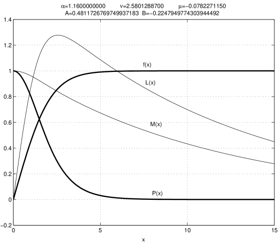
FIG. 1.: The vortex solution. The parameters chosen for this example lie on the surface defining the parameter space of the model and illustrated in Fig. 2.

The requirement of regular geometry in the core of the string reads

$$\left.\frac{dM}{dx}\right|_{0}=0~{},~{}~{}{\cal L}(0)=0~{},~{}~{}\left.\frac{d{\cal L}}{dx}\right|_{0}=1~{},$$ (3.12)

and $M(0)=1$. More specifically, at large distances from the core the behaviour of the geometry is ${\rm AdS}_{6}$ space-time characterized by exponentially decreasing warp factors

$$M(x)\sim e^{-cx},~{}~{}~{}~{}{\cal L}(x)\sim e^{-cx},$$ (3.13)

where $c=\sqrt{-\mu/10}$. This behaviour can be understood since the defects corresponding to the solution of Fig. 1 are local and their related energy-momentum tensor goes to zero at large distances where the geometry is determined only by the value of the bulk cosmological constant.

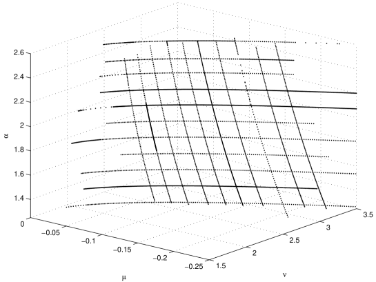
FIG. 2.: The parameter space of the vortex solution is illustrated in terms of the dimension-less parameters reported in Eq. (3.1).

The form of the solutions in the vicinity of the core of the vortex can be studied by expressing the metric functions together with the scalar and gauge fields as a power series in $x$, the dimensionless bulk radius. The power series will then be inserted into Eqs. (3.2)–(3.6). Requiring that the series obeys, for $x\rightarrow 0$, the boundary conditions of Eqs. (3.11) the form of the solutions can be determined as a function of the parameters of the model:

$$f(x) \simeq Ax+\left(\frac{2\mu}{3}+\frac{\nu}{6}+\frac{4B^{2}\nu}{3\alpha}+\frac{2A^{2}\nu}{3}-1+2B\right)\frac{A}{8}x^{3},$$ (3.14)

$$P(x) \simeq 1+Bx^{2},$$ (3.15)

$$M(x) \simeq 1+\left(-\frac{\mu}{8}-\frac{\nu}{32}+\frac{\nu B^{2}}{4\alpha}\right)x^{2},$$ (3.16)

$${\cal L}(x) \simeq x+\left[\frac{\mu}{12}+\nu(\frac{1}{48}-\frac{5B^{2}}{6\alpha}-\frac{A^{2}}{6})\right]x^{3}.$$ (3.17)

In Eq. (3.17) $A$ and $B$ are two arbitrary constants which cannot be determined by the local analysis of the equations of motion. These constants are to be found by boundary conditions for $f(x)$ and $P(x)$ at infinity.

By studying the relations among the string tensions it is possible tro determine the value of $B$ as discussed in detail in [18]. For all the solutions of the family defined by the fine-tuning surface of Fig. 2 we have that

$$-\frac{\nu}{\alpha{\cal L}}\left.\frac{dP}{dx}\right|_{0}=1\,.$$ (3.18)

Since $dP/dx$ is related to the magnetic field on the vortex, Eq. (3.18) tells that in order to have ${\rm AdS}_{6}$ (at infinity) and a local vortex (around the origin) a specific relation among the dimension-less couplings and the value of the magnetic field on the vortex must hold. In fact, according to Eq. (3.17), for $x\rightarrow 0$, $P\sim 1+Bx^{2}$. Using Eq. (3.18), the expression for $B$ can be exactly computed

$$B=-\frac{\alpha}{2\nu}\,.$$ (3.19)

The relation (3.19) among the parameters is satisfied by all the solutions of the type of Fig. 1. This aspect can be appreciated by looking at the specific numerical values of the different parameters reported on top of the plots. The solutions belonging to the family represented by Fig. 1 are regular everywhere, not only in the origin or at infinity. This feature of the solution is illustrated by the behaviour of the curvature invariants which are reported in Fig. 3.

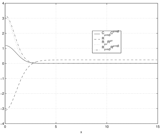
FIG. 3.: The curvature invariants pertaining to the solution of Fig. 1. All the curvature invariants are regular for the class of vortex solutions examined in the present analysis.

While the vortex solutions have been analytically obtained, the asymptotic behaviour of the gauge and Higgs field can be analytically understood in simple terms.

If we expand the gauge and Higgs fields around their boundaries

$$P(x)=\overline{P}+\delta P(x),~{}~{}~{}\overline{P}\sim 0,$$ (3.20)

$$f(x)=\overline{f}-\delta f(x),~{}~{}~{}\overline{f}=1,$$ (3.21)

and if we take into account that, in the same limit, the warp factors decrease exponentially, then we get from Eqs. (3.2)–(3.6)

$$\delta P(x)\sim e^{\sigma_{1}x},\,\,\sigma_{1}=\frac{3c}{2}\bigl{[}1\pm\sqrt{1+\frac{4\alpha}{9c^{2}}}\bigr{]},$$ (3.22)

$$\delta f(x)\sim e^{\sigma_{2}x},\,\,\,\,\sigma_{2}=\frac{5c}{2}\bigl{[}1\pm\sqrt{1+\frac{8}{25c^{2}}}\bigr{]}.$$ (3.23)

If $4\alpha\gg 9c^{2}$ (the limit of small bulk cosmological constant) the solution is compatible with the gauge field decreasing asymptotically as $\delta P\sim e^{-\sqrt{\alpha}x}$. If $25c^{2}<8$ the the perturbed solution goes as $\delta f\sim e^{-\sqrt{2}x}$.

There is an interesting relations which may be derived by direct integration of the equations of motions. Consider the difference between the $(0,0)$ and $(\theta,\theta)$ components of the Einstein equations, i.e. (3.4) and (3.5):

$$\frac{d(H-F)}{dx}+(F+4H)(F-H)=-\nu(\tau_{0}-\tau_{\theta})$$ (3.24)

Multiplying both sides of this equation by $M^{4}{\cal L}$ and integrating from $0$ to $x$ we get

$$(H-F)=\frac{\nu}{\alpha}\frac{P}{{\cal L}^{2}}\frac{dP}{dx}-\biggl{(}1+\left.\frac{\nu}{\alpha{\cal L}}\frac{dP}{dx}\right|_{0}\biggr{)}\frac{1}{M^{4}{\cal L}}.$$ (3.25)

If the tuning among the string tensions is enforced, according to Eqs. (3.18) and (3.19) the boundary term in the core disappears and the resulting equation will be

$$F=H-\frac{\nu}{\alpha}\frac{P~{}}{{\cal L}^{2}}\frac{dP}{dx}.$$ (3.26)

This relation holds for all the family of solutions describing vortex-type solutions with ${\rm AdS}_{6}$ behaviour at infinity and it will turn out to be important for the analysis of the localization properties of the vector fluctuations of the model.

IV Tensor and vector fluctuations of the gravitating vortex

A Tensor fluctuations

The evolution equation for the spin two fluctuations of the geometry are decoupled from the very beginning and they are easily obtained from the tensor component of the perturbed Einstein equations, namely from Eq. (2.31). The details are reported in Appendix A and the final result is

$$h_{\mu\nu}^{\prime\prime}+\frac{1}{{\cal L}^{2}}\ddot{h}_{\mu\nu}+(4H+F)h_{\mu\nu}^{\prime}-\frac{2}{m_{H}^{2}M^{2}}\Box h_{\mu\nu}=0.$$ (4.1)

For the lowest mass eigenstate (i.e. $\Box h_{\mu\nu}=0$ and $\ddot{h}_{\mu\nu}=0$), Eq. (4.1) admit a solution with constant amplitude. Denoting with $h$ each polarization, the constant zero mode will be $h=K$ where $K$ is a constant.

In order to discuss the localization properties of the zero mode, the canonically normalized kinetic term (coming from the action perturbed to second order) should be derived. Going to the action of the tensor fluctuation the canonical variable

$$q=M\sqrt{L}h,$$ (4.2)

can be read-off. In terms of $q$ the kinetic term of the tensor fluctuations is canonically normalized and the corresponding normalization integral is then

$$K^{2}\int_{0}^{\infty}M^{2}(x){\cal L}(x)dx.$$ (4.3)

The requirement that the integral (4.3) is finite corresponds to the requirement that the four-dimensional Planck mass is finite. In fact, Eq. (1.2) can be also written as

$$M_{P}^{2}=\frac{4\pi}{m_{H}^{2}}M^{4}_{6}\int_{0}^{\infty}dxM^{2}(x){\cal L}(x).$$ (4.4)

Therefore, if the four-dimensional Planck mass is finite also the tensor zero mode is normalizable. Furthermore, using the asymptotics of the background solutions reported in Eqs. (3.17) and (3.13) the following behaviour of the canonically normalized zero mode can be obtained:

$$q(x)\sim e^{-\frac{3}{2}cx},~{}~{}~{}~{}~{}x\to\infty$$ (4.5)

$$q(x)\sim\sqrt{x},~{}~{}~{}~{}~{}~{}~{}~{}~{}~{}x\to 0.$$ (4.6)

As a consequence, the normalization integral (4.3) as well as (4.4) will always give finite results. These findings are in full agreement with the ones reported in [17] with the difference that, in the present case, we are dealing with an explicit model of vortex based on the Abelian-Higgs model. The reason why tensor fluctuations can be analyzed even without an explicit model, is that they decouple mfrom the sources. The same statement cannot be made for the vector modes of the geometry whose coupling to the sources is essential, as it will be now discussed.

B Vector fluctuations

In terms of the gauge-invariant quantities defined in Section II the evolution equations for the vector modes of the system can be derived from Eqs. (2.32)–(2.34) and from Eq. (2.36). While the detailed derivation is reported in Appendix A, the final result of the straightforward but lengthy algebra is the following

$$V_{\mu}^{\prime}+(3H+F)V_{\mu}+\frac{\dot{Z}_{\mu}}{{\cal L}}=0,$$ (4.7)

$$\frac{\ddot{V}_{\mu}}{{\cal L}^{2}}-\frac{2}{m_{H}^{2}~{}M^{2}}\Box V_{\mu}-\frac{\dot{Z}_{\mu}^{\prime}}{{\cal L}}+(H-F)\frac{\dot{Z}_{\mu}}{{\cal L}}=2\frac{L}{M}\frac{\nu}{\alpha}\frac{P^{\prime}}{{\cal L}^{2}}\frac{\dot{{\cal A}}_{\mu}}{{\cal L}},$$ (4.8)

$$Z_{\mu}^{\prime\prime}+(4H+F)Z_{\mu}^{\prime}+(F^{\prime}-H^{\prime}+5HF-5H^{2})Z_{\mu}-\frac{2}{m_{H}^{2}~{}M^{2}}\Box Z_{\mu}$$ (4.9)

$$-\frac{1}{{\cal L}}\biggl{[}\dot{V}_{\mu}^{\prime}+(5H-F)\dot{V}_{\mu}\biggr{]}+2\frac{L}{M}\biggl{(}\frac{\nu}{\alpha}\frac{P^{\prime}}{{\cal L}^{2}}{\cal A}_{\mu}^{\prime}+\frac{\nu Pf^{2}}{{\cal L}^{2}}{\cal A}_{\mu}\biggr{)}=0,$$ (4.10)

$${\cal A}_{\mu}^{\prime\prime}+\frac{\ddot{{\cal A}}_{\mu}}{{\cal L}^{2}}-\frac{2}{m_{H}^{2}~{}M^{2}}\Box{\cal A}_{\mu}+(2H+F){\cal A}_{\mu}^{\prime}$$ (4.11)

$$-P^{\prime}\frac{M}{L}\biggl{[}Z_{\mu}^{\prime}-(H-F)Z_{\mu}-\frac{\dot{V}_{\mu}}{{\cal L}}\biggr{]}-\alpha{\cal A}_{\mu}f^{2}=0.$$ (4.12)

This system defines the evolution of the three gauge-invariant vector fluctuations appearing in the gravitating Abelian Higgs model, namely $V_{\mu}$, $Z_{\mu}$ and ${\cal A}_{\mu}$. These three vectors are divergence-less and have been defined in Eqs. (2.24)–(2.25) and in eq. (2.30). While Eq. (4.7) is a constraint, the other equations are all dynamical.

In order to simplify the above system it is useful to introduce the following combination of the derivatives of the two graviphoton fields namely: Define now the following variable

$$u_{\mu}=\varepsilon\frac{\dot{V}_{\mu}}{{\cal L}}-(\varepsilon Z_{\mu})^{\prime},$$ (4.13)

where $\varepsilon$ is a background function satisfying

$$\varepsilon=\frac{L}{M},~{}~{}~{}~{}~{}~{}~{}\frac{\varepsilon^{\prime}}{\varepsilon}=F-H.$$ (4.14)

Using Eq. (4.13), Eqs. (4.7)–(4.12) can then be written in a more compact form, namely:

$$V_{\mu}^{\prime}+(4H+\frac{\varepsilon^{\prime}}{\varepsilon})V_{\mu}+\frac{\dot{Z}_{\mu}}{{\cal L}}=0,$$ (4.15)

$$\frac{\dot{u}_{\mu}}{{\cal L}}-\frac{2}{m_{H}^{2}}\frac{\varepsilon}{M^{2}}\Box V_{\mu}=2\varepsilon^{2}\frac{\nu}{\alpha}P^{\prime}\frac{\dot{{\cal A}}_{\mu}}{{\cal L}},$$ (4.16)

$$u_{\mu}^{\prime}+(5H-\frac{\varepsilon^{\prime}}{\varepsilon})u_{\mu}+2\frac{\varepsilon}{m_{H}^{2}M^{2}}\Box Z_{\mu}=2\varepsilon^{2}\biggl{[}\frac{\nu}{\alpha}\frac{P^{\prime}}{{\cal L}^{2}}{\cal A}_{\mu}^{\prime}+\frac{\nu Pf^{2}}{{\cal L}^{2}}{\cal A}_{\mu}\biggr{]},$$ (4.17)

$${\cal A}_{\mu}^{\prime\prime}+\frac{\ddot{{\cal A}}_{\mu}}{{\cal L}^{2}}-\frac{2}{m_{H}^{2}~{}M^{2}}\Box{\cal A}_{\mu}+(2H+F){\cal A}_{\mu}^{\prime}+\frac{P^{\prime}}{\varepsilon^{2}}u_{\mu}-\alpha f^{2}{\cal A}_{\mu}=0.$$ (4.18)

In order to determine the zero modes of the system consider first the case where the mass of $V_{\mu}$ vanishes, i.e. $\Box V_{\mu}=0$. In this case from Eq. (4.16) the following relation holds:

$$u_{\mu}=2\varepsilon^{2}\frac{\nu}{\alpha}\frac{P^{\prime}}{{\cal L}^{2}}{\cal A}_{\mu}.$$ (4.19)

Inserting Eq. (4.19) into Eq. (4.18) the equation for the gauge field fluctuation can be simplified with the result that

$${\cal A}_{\mu}^{\prime\prime}+\frac{\ddot{{\cal A}}_{\mu}}{{\cal L}^{2}}-\frac{2}{m_{H}^{2}~{}M^{2}}\Box{\cal A}_{\mu}+(2H+F){\cal A}_{\mu}^{\prime}+\biggl{[}2\frac{\nu}{\alpha}\frac{{P^{\prime}}^{2}}{{\cal L}^{2}}-\alpha f^{2}\biggr{]}{\cal A}_{\mu}=0.$$ (4.20)

Already from this expression we can see that the zero mode of ${\cal A}_{\mu}$ will not be constant but it will be a function of the bulk radius. This property is in contrast with the results obtained in the case of the tensor zero mode. In order to solve explicitely for the zero mode Eq. (4.20) can be further simplified by using the equations of motion of the background. In particular, from Eq. (3.2) we have that

$$\alpha f^{2}=\frac{P^{\prime\prime}}{P}+(4H-F)\frac{P^{\prime}}{P},$$ (4.21)

whereas, using Eq. (3.26) we also have that

$$2\frac{\nu}{\alpha}\frac{{P^{\prime}}^{2}}{{\cal L}^{2}}=(H-F)\frac{P^{\prime}}{P}.$$ (4.22)

Inserting Eqs. (4.21) and (4.22) into the last term of Eq. (4.20) the following equation can be obtained, namely

$${\cal A}_{\mu}^{\prime\prime}+\frac{\ddot{{\cal A}}_{\mu}}{{\cal L}^{2}}-\frac{2}{m_{H}^{2}~{}M^{2}}\Box{\cal A}_{\mu}+(2H+F){\cal A}_{\mu}^{\prime}-\biggl{[}\frac{P^{\prime\prime}}{P}+(2H+F)\frac{P^{\prime}}{P}\biggr{]}{\cal A}_{\mu}=0.$$ (4.23)

Finally, defining the appropriately rescaled variable,

$$b_{\mu}=M\sqrt{L}{\cal A}_{\mu}$$ (4.24)

the first derivative with respect to the bulk radius can be eliminated from Eq. (4.23) with the result that

$$b_{\mu}^{\prime\prime}+\frac{\ddot{b}_{\mu}}{{\cal L}^{2}}-\frac{2}{m_{H}^{2}M^{2}}\Box b_{\mu}-\frac{(M\sqrt{L}P)^{\prime\prime}}{M\sqrt{L}P}b_{\mu}=0,$$ (4.25)

From Eq. (4.25) the corresponding zero mode can be easily obtained. Expanding the excitation in Fourier series with respect to $\theta$ and in Fourier integral with respect to the four-momentum

$$b_{\mu}(x^{\mu},\theta,w)=\sum_{\ell=-\infty}^{+\infty}\int e^{ipx}d^{4}p~{}b_{\mu}(\ell,p,w).$$ (4.26)

Hence, in Eq. (4.25) the D’Alembertian is replaced by $-m^{2}$ and the term containing the double derivative with respect to $\theta$ is replaced by $-\ell^{2}$. The lowest mass and angular momentum eigenstates will then obey the following equation for the zero mode

$$b_{\mu}^{\prime\prime}-\frac{(M\sqrt{L}P)^{\prime\prime}}{M\sqrt{L}P}b_{\mu}=0.$$ (4.27)

whose solution, in terms of ${\cal A}_{\mu}$ can be written as

$${\cal A}_{\mu}(x)=k_{1,\mu}P(x),$$ (4.28)

where $k_{1,\mu}$ is an integration constant which should be determined by normalizing the canonical zero mode associated with gauge field fluctuations. As anticipated this zero mode is a specific function of the bulk radius and not a constant. More specifically, according to Eqs. (3.17)–(3.19) and (3.22),

$${\cal A}_{\mu}(x)\simeq 1-\frac{\alpha}{2\nu}x^{2},~{}~{}~{}~{}x\to 0,$$ (4.29)

$${\cal A}_{\mu}(x)\simeq e^{-\sqrt{\alpha}x},~{}~{}~{}~{}x\to\infty.$$ (4.30)

Hence, the zero mode of Eq. (4.28) satisfies the correct boundary conditions since

$${\cal A}_{\mu}^{\prime}(0)={\cal A}_{\mu}^{\prime}(\infty)=0,$$ (4.31)

so that the differential operator of Eq. (4.23) is self-adjoint.

Inserting Eq. (4.19) into Eq. (4.17)( or (4.10), the obtained equation implies that

$$\Box Z_{\mu}=0,$$ (4.32)

so that also the second graviphoton field should have zero mass. In order to determine the explicit expressions of the zero modes related to $V_{\mu}$ and $Z_{\mu}$ we should consider radial excitations. Thus, inserting Eq. (4.28) into Eq. (4.19) and recalling Eq. (4.13) the zero mode for $Z_{\mu}$ can be obtained

$$Z_{\mu}(x)=k_{1,\mu}\frac{L(x)}{M(x)}+c_{2,\mu}\frac{M(x)}{L(x)},$$ (4.33)

where $c_{2,\mu}$ is a further integration constant. From Eq. (4.15) the zero mode of $V_{\mu}$ turns out to be

$$V_{\mu}(x)=\frac{c_{1,\mu}}{M^{3}(x)L(x)},$$ (4.34)

where $c_{1,\mu}$ is the integration constant.

By now perturbing the action to second order the correct canonical normalization of the fields can be deduced. The canonical fields related to ${\cal A}_{\mu}$, $V_{\mu}$ and $Z_{\mu}$ are

$$\overline{{\cal A}}_{\mu}=\sqrt{L}{\cal A}_{\mu},$$ (4.35)

$$\overline{V}_{\mu}=M\sqrt{L}V_{\mu},$$ (4.36)

$$\overline{Z}_{\mu}=M\sqrt{L}Z_{\mu}.$$ (4.37)

In order to get to Eqs. (4.37), it is better to perturb to second order the Einstein-Hilbert action directly in the form [29]

$$G^{AB}\biggl{(}\Gamma_{AC}^{D}\Gamma_{BD}^{C}-\Gamma_{AB}^{C}\Gamma_{CD}^{D}\biggr{)}$$ (4.38)

where the total derivatives are absent. Using the results of Section III, and, in particular, Eqs. (3.17) and (3.22) the canonically normalized gauge zero mode behaves, asymptotically, as

$$\overline{{\cal A}}_{\mu}(x)\sim e^{-(\frac{c}{2}+\sqrt{\alpha})x},~{}~{}~{}~{}~{}~{}x\to\infty,$$ (4.39)

$$\overline{{\cal A}}_{\mu}(x)\sim\sqrt{x},~{}~{}~{}~{}~{}x\to 0$$ (4.40)

The canonically normalized graviphoton fields will behave, asymptotically, as

$$\overline{V}_{\mu}(x)\sim e^{\frac{3}{2}x},~{}~{}~{}~{}~{}~{}~{}~{}x\to\infty,$$ (4.41)

$$\overline{V}_{\mu}(x)\sim\frac{1}{\sqrt{x}},~{}~{}~{}~{}~{}~{}~{}x\to 0,$$ (4.42)

and

$$\overline{Z}_{\mu}(x)\sim e^{-\frac{3}{2}x},~{}~{}~{}~{}~{}~{}x\to\infty,$$ (4.43)

$$\overline{Z}_{\mu}(x)\sim\frac{1}{\sqrt{x}},~{}~{}~{}~{}~{}~{}~{}x\to 0.$$ (4.44)

Consider now the normalization integrals. For the gauge field zero mode the normalization integral is

$$\int_{0}^{\infty}~{}dx|\overline{{\cal A}}_{\mu}(x)|^{2}=|k_{1,\mu}|^{2}\int_{0}^{\infty}L(x)P^{2}(x)dx.$$ (4.45)

From Eqs. (4.40) and from the explicit solutions where the asymptotics are realized, the integral of (4.45) always give a finite result. More specifically the integrand goes always as $x$ for $x\to 0$ and it is exponentially suppressed for $x\to\infty$. It should be appreciated that this result has been derived only using the equations of motion of the background and of the fluctuations. In other words the asymptotic beahaviour of the vortex solution is not specific of a given set of parameters but it is generic for the class of solutions discussed in Section III.

For the gauge-invariant vector fluctuations of the metric the normalization integrals are:

$$\int_{0}^{\infty}~{}dx|\overline{V}_{\mu}(x)|^{2}=|c_{1,\mu}|^{2}\int_{0}^{\infty}\frac{dx}{M^{4}(x)L(x)},$$ (4.46)

$$\int_{0}^{\infty}~{}dx|\overline{Z}_{\mu}(x)|^{2}=\int_{0}^{\infty}\biggl{[}|k_{1,\mu}|^{2}L^{3}(x)+|c_{2,\mu}|^{2}\frac{M^{4}(x)}{L(x)}+2k_{1,\mu}c_{1,\mu}M^{2}(x)L(x)\biggr{]}dx.$$ (4.47)

Consider first Eq. (4.46). Since for $x\to\infty$ the warp factors are exponentially decreasing the integrand of Eq. (4.46) diverges. This can be appreciated also from Eq. (4.42) whose square is the integrand appearing in (4.46). Hence, the zero mode of $V_{\mu}$ is never localized. Finally the second term of the integrand of Eq. (4.47) diverges as $1/x$ for $x\to 0$ leading to an integral which is logarithmically divergent in the same limit. Again, this can be also appreciated from Eqs. (4.44). As a consequence, none of the graviphoton fields are localized since their related normalization integrals are always divergent either close to the core of the defect, or at infinity.

V Conclusions

In this paper the vector and tensor fluctuations of the six-dimensional Abelian-Higgs model have been considered. Thanks to the presence of a negative cosmological constant in the bulk the vortex solutions appearing in this framework lead to gravity localization and to a finite four-dimensional Planck mass. Since the four-dimensional Planck mass is finite, also the graviton zero mode is always localized.

A different situation occurs for the vector fluctuations of the geometry whose normalization integrals lead to the following two conditions, namely,

$$|c_{1,\mu}|^{2}\int_{0}^{\infty}\frac{dx}{M^{4}(x)L(x)},$$ (5.1)

$$\int_{0}^{\infty}\biggl{[}|k_{1,\mu}|^{2}L^{3}(x)+|c_{2,\mu}|^{2}\frac{M^{4}(x)}{L(x)}+2k_{1,\mu}c_{1,\mu}M^{2}(x)L(x)\biggr{]}dx.$$ (5.2)

Since the convergence of the four-dimensional Planck mass implies that

$$\int_{0}^{\infty}M^{2}(x)L(x)dx,$$ (5.3)

is always finite, then the integral of (5.1) will diverge at infinity. Since the regularity of the geometry close to the core of the vortex implies that

$${\cal L}(x)=\sqrt{\lambda}vL(x)\sim x,~{}~{}~{}~{}~{}M(x)\sim 1,$$ (5.4)

for $x\to 0$, then the integral of (5.2) will be divergent for $x\to 0$.

An intriguing result, which should be further scrutinized, holds for the gauge zero mode whose normalization integral implies that

$$|k_{1,\mu}|^{2}\int_{0}^{\infty}L(x)P^{2}(x)dx,$$ (5.5)

should be finite. The local nature of the string-like defect demands, for the solutions localizing gravity presented in this paper, that $P(x)\to 1$ for $x\to 0$ and $P(x)\sim e^{-\sqrt{\alpha}x}$ for $x\to\infty$. This observation together with the regularity of the geometry in the core of the vortex, implies that the same solutions leading to gravity localization, also lead to the localization of the gauge zero mode. Notice that if the cosmological constant does not vanish, $\alpha=e^{2}/\lambda>1$. In fact, in the limit of zero cosmological constant (i.e. $\mu\to 0$ in our notations), $\alpha$ goes to $2$ [18] and the Bogomolnyi limit is recovered .

It should be appreciated that the obtained results have been derived in general terms. First of all they are independent on the specific coordinate system since a fully gauge-invariant derivation as been employed. Second, the obtained results hold for all the class of backgrounds localizing gravity in the six-dimensional Abelian Higgs model. In fact, even if specific background solutions have been presented and used in order to illustrate the results, the zero modes have been computed without assuming any specific solution.

In order to interpret the localized gauge zero mode as an electromagnetic degree of freedom, the inclusion of fermions in the model is mandatory. This is the reason why we cannot claim that our findings support a mechanism for the localization of electromagnetic interactions on a string-like defect in higher dimensions. In order to address precisely this point it would be interesting to use recent results concerning fermionic degrees of freedom on six-dimensional vortices [11, 12, 30].

A Gauge-invariant fluctuations of the gravitating vortex

In the following the explicit expressions of the various fluctuations needed for the derivations presented in the bulk of the paper will be reported. The background values of the Christoffel connections are

$$\overline{\Gamma}_{\alpha\rho}^{\beta}=\sqrt{\lambda}~{}v~{}H\delta_{\alpha}^{\beta},$$ (A.1)

$$\overline{\Gamma}_{\alpha\beta}^{\rho}=\sqrt{\lambda}~{}v~{}M^{2}~{}H\eta_{\alpha\beta},$$ (A.2)

$$\overline{\Gamma}_{\rho\theta}^{\theta}=\sqrt{\lambda}~{}v~{}F,$$ (A.3)

$$\overline{\Gamma}_{\theta\theta}^{\rho}=-\sqrt{\lambda}~{}v~{}L^{2}F.$$ (A.4)

Notice that $\rho$ and $\theta$ denote the two transverse coordinates whereas the other Greek letters label the four space-time coordinates. Notice, furthermore, that as indicated in the bulk of the paper, the prime denotes the derivation with respect to $x=\sqrt{\lambda}v\rho$, and the overdot the derivative with respect to $\theta$. As it is apparent from expressions of the evolution equations of the fluctuations, the use of the $x$ and $\theta$ (instead of $\rho$ and $\theta$) makes the whole discussion simpler.

Using Eq. (2.21) the first order fluctuations of the Christoffel connections are easily obtained :

$$\delta^{(1)}\Gamma_{\mu\nu}^{\rho}=\sqrt{\lambda}~{}v~{}M^{2}[H_{\mu\nu}^{\prime}+2HH_{\mu\nu}]-M\partial_{(\mu}D_{\nu)},$$ (A.5)

$$\delta^{(1)}\Gamma_{\rho\mu}^{\rho}=\sqrt{\lambda}~{}v~{}M~{}HD_{\mu},$$ (A.6)

$$\delta^{(1)}\Gamma_{\mu\theta}^{\rho}=\frac{\sqrt{\lambda}~{}v}{2}~{}ML[Q_{\mu}^{\prime}+(H+F)Q_{\mu}]-\frac{M}{2}\dot{D}_{\mu},$$ (A.7)

$$\delta^{(1)}\Gamma_{\mu\nu}^{\theta}=\frac{M^{2}}{L^{2}}\dot{H}_{\mu\nu}-\frac{M}{L}\partial_{(\mu}Q_{\nu)},$$ (A.8)

$$\delta^{(1)}\Gamma_{\mu\rho}^{\theta}=\frac{M}{2L^{2}}\dot{D}_{\mu}-\sqrt{\lambda}v\frac{M}{2L}[Q_{\mu}^{\prime}+Q_{\mu}(F-H)]$$ (A.9)

$$\delta^{(1)}\Gamma_{\alpha\beta}^{\mu}=-\sqrt{\lambda}~{}v~{}HMD^{\mu}\eta_{\alpha\beta}+(\partial_{\alpha}H_{\beta}^{~{}\mu}+\partial_{\beta}H_{\alpha}^{~{}\mu}-\partial^{\mu}H_{\alpha\beta}),$$ (A.10)

$$\delta^{(1)}\Gamma_{\alpha\rho}^{\mu}=\frac{1}{2M}(\partial_{\alpha}D^{\mu}-\partial^{\mu}D_{\alpha})+\sqrt{\lambda}~{}v~{}{H_{\alpha}^{\mu}}^{\prime},$$ (A.11)

$$\delta^{(1)}\Gamma_{\theta\theta}^{\mu}=\frac{L}{M}\dot{Q}^{\mu}+\sqrt{\lambda~{}v}\frac{L^{2}}{M}~{}FD^{\mu},$$ (A.12)

$$\delta^{(1)}\Gamma_{\alpha\theta}^{\mu}=\frac{L}{2M}(\partial_{\alpha}Q^{\mu}-\partial^{\mu}Q_{\alpha})+\dot{H}_{\alpha}^{~{}\mu},$$ (A.13)

$$\delta^{(1)}\Gamma_{\rho\rho}^{\mu}=\frac{\sqrt{\lambda}~{}v}{M}[{D^{\mu}}^{\prime}+HD^{\mu}],$$ (A.14)

$$\delta^{(1)}\Gamma_{\theta\rho}^{\mu}=\sqrt{\lambda}~{}v~{}\frac{L}{2M}[{Q^{\mu}}^{\prime}+(H-F)Q^{\mu}]+\frac{\dot{D}^{\mu}}{2M},$$ (A.15)

where, for short,

$$H_{\mu\nu}=h_{\mu\nu}+\partial_{(\mu}f_{\nu)}.$$ (A.16)

With the use of Eqs. (A.4) and (A.15), Eq. (2.37) allows the explicit determination of the first order Ricci fluctuations:

$$\delta^{(1)}R_{\mu\nu} = \lambda~{}v^{2}M^{2}[H_{\mu\nu}^{\prime\prime}+(4H+F)H_{\mu\nu}^{\prime}+H_{\mu\nu}(2H^{\prime}+8H^{2}+2HF)]+\frac{M^{2}}{L^{2}}\ddot{H}_{\mu\nu}$$ (A.17)

$$- \partial_{\alpha}\partial^{\alpha}H_{\mu\nu}+(\partial_{\alpha}\partial_{\mu}H_{\nu}^{\alpha}+\partial_{\alpha}\partial_{\nu}H_{\mu}^{\alpha}+\partial_{\nu}\partial^{\alpha}H_{\alpha\mu}-\partial_{\nu}\partial_{\alpha}H_{\mu}^{\alpha}),$$ (A.18)

$$- \sqrt{\lambda}~{}v~{}M[\partial_{(\mu}D_{\nu)}^{\prime}+(3H+F)\partial_{(\mu}D_{\nu)}]-\frac{M}{L}\partial_{(\mu}\dot{Q}_{\nu)},$$ (A.19)

$$\delta^{(1)}R_{\mu\rho} = \frac{M}{2L^{2}}\ddot{D}_{\mu}-\frac{M}{2L}\sqrt{\lambda}~{}v~{}[\dot{Q}^{\prime}_{\mu}+(F-H)\dot{Q}_{\mu}]-\frac{1}{2M}\partial_{\alpha}\partial^{\alpha}D_{\mu}$$ (A.20)

$$+ \lambda~{}v^{2}M[H^{\prime}+4H^{2}+HF]D_{\mu}+\sqrt{\lambda}~{}vH_{\mu\alpha}^{\prime},$$ (A.21)

$$\delta^{(1)}R_{\mu\theta} = \partial^{\alpha}\dot{H}_{\alpha\mu}-\frac{L}{2M}\partial_{\alpha}\partial^{\alpha}Q_{\mu}-\frac{\sqrt{\lambda}~{}v}{2}~{}M[\dot{D}_{\mu}^{\prime}+(5H-F)\dot{D}_{\mu}]$$ (A.22)

$$+ \lambda~{}v^{2}~{}\frac{ML}{2}[Q_{\mu}^{\prime\prime}+(4H+F)Q_{\mu}^{\prime}+(H^{\prime}+F^{\prime}+3H^{2}+7HF)Q_{\mu}].$$ (A.23)

The first order fluctuations of $\tau_{AB}$ defined in Eq. (2.9) and appearing at the right hand side of Eqs. (2.32)–(2.34) can be also computed and they are

$$\kappa\delta^{(1)}\tau_{\mu\nu} = \lambda~{}v^{2}M^{2}\biggl{[}-\mu+\frac{\nu}{2\alpha}\frac{P^{\prime 2}}{{\cal L}^{2}}-\frac{\nu}{4}(f^{2}-1)^{2}\biggr{]}H_{\mu\nu},$$ (A.24)

$$\kappa\delta^{(1)}\tau_{\mu\rho} = \lambda~{}v^{2}M\biggl{[}-\frac{\mu}{2}+\frac{\nu}{4\alpha}\frac{P^{\prime 2}}{{\cal L}^{2}}-\frac{\nu}{8}(f^{2}-1)^{2}\biggr{]}D_{\mu}+\sqrt{\lambda}~{}v~{}\frac{\nu}{\alpha}\frac{P^{\prime}}{{\cal L}^{2}}\dot{{\cal A}}_{\mu},$$ (A.25)

$$\kappa\delta^{(1)}\tau_{\mu\theta} = \lambda v^{2}ML\biggl{[}-\frac{\mu}{2}+\frac{\nu}{4\alpha}\frac{P^{\prime 2}}{{\cal L}^{2}}-\frac{\nu}{8}(f^{2}-1)^{2}\biggr{]}Q_{\mu}-\frac{\nu}{\alpha}P^{\prime}{\cal A}_{\mu}^{\prime}-\nu Pf^{2}{\cal A}_{\mu}.$$ (A.26)

In order to obtain the evolution equations written explicitly in terms of the gauge-invariant fluctuations we recall that while $h_{\mu\nu}$ and ${\cal A}_{\mu}$ are already gauge-invariant, $f_{\mu}$, $D_{\mu}$ and $Q_{\mu}$ change for infinitesimal coordinate transformation according to Eqs. (2.23)–(2.25).

The evolution equations of the fluctuations will now be written in fully gauge-invariant terms. The strategy will be the, in short, the following. By using Eqs. (2.26) and (2.27), the first order fluctuations of the Ricci tensors can be expressed in terms of a gauge-invariant part plus a gauge-dependent piece. The same procedure can be carried on in the case of the fluctuations of the energy-momentum tensor. When the Einstein’s equations are explicitly written to first order in the amplitude of the metric fluctuations as,

$$\delta^{(1)}R_{AB}=\kappa\delta^{(1)}\tau_{AB}$$ (A.27)

the gauge-dependent parts vanish, identically, by using the equations of motion of the background reported in Eqs. (3.2)–(3.6).

From Eqs. (2.24)–(2.25) we can write

$$D_{\mu} = V_{\mu}+\sqrt{\lambda}~{}v~{}Mf_{\mu}^{\prime}$$ (A.28)

$$Q_{\mu} = Z_{\mu}+\frac{M}{L}\dot{f}_{\mu}.$$ (A.29)

Using Eqs. (A.29) into Eqs. (A.19)–(A.23) and (A.24)–(A.26) the following first order fluctuations can be obtained

$$\delta^{(1)}R_{\mu\nu} = \lambda v^{2}M^{2}[h_{\mu\nu}^{\prime\prime}+(4H+F)h_{\mu\nu}^{\prime}+(2H^{\prime}+8H^{2}+2HF)h_{\mu\nu}]+\frac{M^{2}}{L^{2}}\ddot{h}_{\mu\nu}-\partial_{\alpha}\partial^{\alpha}h_{\mu\nu}$$ (A.30)

$$- \sqrt{\lambda}~{}v~{}M[\partial_{(\mu}V_{\nu)}^{\prime}+(3H+F)\partial_{(\mu}V_{\nu)}]-\frac{M}{L}\partial_{(\mu}\dot{Z}_{\nu)}$$ (A.31)

$$+ \lambda v^{2}M^{2}(2H^{\prime}+8H^{2}+2HF)\partial_{(\mu}f_{\nu)},$$ (A.32)

$$\delta^{(1)}R_{\mu\rho} = \frac{M}{2L^{2}}\ddot{V}_{\mu}-\frac{M}{2L}\sqrt{\lambda}~{}v[\dot{Z}_{\mu}^{\prime}+\dot{Z}_{\mu}(F-H)]$$ (A.33)

$$- \frac{1}{2M}\partial_{\alpha}\partial^{\alpha}V_{\mu}+\lambda v^{2}MV_{\mu}[H^{\prime}+4H^{2}+HF]$$ (A.34)

$$+ (\sqrt{\lambda}v)^{3}~{}M^{2}[H^{\prime}+4H^{2}+HF]f_{\mu}^{\prime},$$ (A.35)

$$\delta^{(1)}R_{\mu\theta} = -\frac{L}{2M}\partial_{\alpha}\partial^{\alpha}Z_{\mu}+\lambda v^{2}\frac{ML}{2}[Z_{\mu}^{\prime\prime}+(4H+F)Z_{\mu}^{\prime}+Z_{\mu}(H^{\prime}+F^{\prime}+3H^{2}+7HF)]$$ (A.36)

$$- \frac{\sqrt{\lambda}v}{2}M[\dot{V}_{\mu}^{\prime}+(5H-F)\dot{V}_{\mu}]+\lambda v^{2}M^{2}(H^{\prime}+4H^{2}+HF)\dot{f}_{\mu},$$ (A.37)

and

$$\kappa\delta^{(1)}\tau_{\mu\nu} = \lambda v^{2}M^{2}(2H^{\prime}+8H^{2}+2HF)h_{\mu\nu}+\lambda v^{2}M^{2}\partial_{(\mu}f_{\nu)}(2H^{\prime}+8H^{2}+2HF),$$ (A.38)

$$\kappa\delta^{(1)}\tau_{\mu\rho} = \lambda v^{2}M(H^{\prime}+4H^{2}+HF)V_{\mu}+\frac{\nu}{\alpha}\sqrt{\lambda}~{}v\frac{P^{\prime}}{{\cal L}^{2}}\dot{{\cal A}}_{\mu}$$ (A.39)

$$+ (\sqrt{\lambda}v)^{3}M^{2}(H^{\prime}+4H^{2}+HF)f_{\mu}^{\prime},$$ (A.40)

$$\kappa\delta^{(1)}\tau_{\mu\theta} = \lambda v^{2}ML(H^{\prime}+4H^{2}+HF)Z_{\mu}-\frac{\nu}{\alpha}P^{\prime}{\cal A}_{\mu}^{\prime}-\nu Pf^{2}{\cal A}_{\mu}$$ (A.41)

$$+ \lambda v^{2}M^{2}[H^{\prime}+4H^{2}+HF]\dot{f}_{\mu}.$$ (A.42)

Notice that in order to write Eqs. (A.32)–(A.37) and (A.38)–(A.42) the following expression (following from the sum of Eqs. (3.5) and (3.6) ) has been used:

$$2H^{\prime}+8H^{2}+2HF=-\mu-\frac{\nu}{4}(f^{2}-1)^{2}+\frac{\nu}{2\alpha}\frac{P^{\prime 2}}{{\cal L}^{2}}.$$ (A.43)

In each of Eqs. (A.32)–(A.37) and (A.38)–(A.42) the last term is not gauge-invariant. However, imposing Eq. (A.27) all the gauge-dependent pieces cancel and, at the end, the following system of equations is obtained:

$$V_{\mu}^{\prime}+(3H+F)V_{\mu}+\frac{\dot{Z}_{\mu}}{{\cal L}}=0,$$ (A.44)

$$\frac{\ddot{V}_{\mu}}{{\cal L}^{2}}-\frac{2}{m_{H}^{2}~{}M^{2}}\Box V_{\mu}-\frac{\dot{Z}^{\prime}_{\mu}}{{\cal L}}+(H-F)\frac{\dot{Z}_{\mu}}{{\cal L}}=2\frac{L}{M}\frac{\nu}{\alpha}\frac{P^{\prime}}{{\cal L}^{2}}\frac{\dot{{\cal A}}_{\mu}}{{\cal L}},$$ (A.45)

$$Z_{\mu}^{\prime\prime}+(4H+F)Z_{\mu}^{\prime}+(F^{\prime}-H^{\prime}+5HF-5H^{2})Z_{\mu}-\frac{2}{m_{H}^{2}~{}M^{2}}\Box Z_{\mu}$$ (A.46)

$$-\frac{1}{{\cal L}}\biggl{[}\dot{V}_{\mu}^{\prime}+(5H-F)\dot{V}_{\mu}\biggr{]}+2\frac{L}{M}\biggl{(}\frac{\nu}{\alpha}\frac{P^{\prime}}{{\cal L}^{2}}{\cal A}_{\mu}^{\prime}+\frac{\nu Pf^{2}}{{\cal L}^{2}}{\cal A}_{\mu}\biggr{)}=0,$$ (A.47)

for the vector fluctuations and

$$h_{\mu\nu}^{\prime\prime}+\frac{\ddot{h}_{\mu\nu}}{{\cal L}^{2}}+(4H+F)h_{\mu\nu}^{\prime}-\frac{2}{m_{H}^{2}M^{2}}\Box h_{\mu\nu}=0,$$ (A.48)

for the tensor fluctuations.

This system of equations has to be supplemented with the fluctuation of the gauge field equation reported in Eq. (2.36). The pure vector component of the perturbed evolution equation for the gauge field reads:

$${\cal A}_{\mu}^{\prime\prime}+\frac{\ddot{{\cal A}}_{\mu}}{{\cal L}^{2}}-\frac{2}{m_{H}^{2}~{}M^{2}}\Box{\cal A}_{\mu}+(2H+F){\cal A}_{\mu}^{\prime}$$ (A.49)

$$-P^{\prime}\frac{M}{L}\biggl{[}Q_{\mu}^{\prime}-(H-F)Q_{\mu}-\frac{\dot{D}_{\mu}}{{\cal L}}\biggr{]}-\alpha{\cal A}_{\mu}f^{2}=0.$$ (A.50)

In this equation the terms containing ${\cal A}_{\mu}$ are gauge-invariant. The terms containing $Q_{\mu}$ and $D_{\mu}$ are not automatically gauge-invariant. However, using Eqs. (A.29) the following result holds :

$$Q_{\mu}^{\prime}-(H-F)Q_{\mu}-\frac{\dot{D}_{\mu}}{{\cal L}}=Z_{\mu}^{\prime}-(H-F)Z_{\mu}-\frac{\dot{V}_{\mu}}{{\cal L}},$$ (A.51)

and the dependence upon $f_{\mu}$ disappears, as it should. Therefore the final equation for the perturbed gauge field fluctuation is simply

$${\cal A}_{\mu}^{\prime\prime}+\frac{\ddot{{\cal A}}_{\mu}}{{\cal L}^{2}}-\frac{2}{m_{H}^{2}~{}M^{2}}\Box{\cal A}_{\mu}+(2H+F){\cal A}_{\mu}^{\prime}$$ (A.52)

$$-P^{\prime}\frac{M}{L}\biggl{[}Z_{\mu}^{\prime}-(H-F)Z_{\mu}-\frac{\dot{V}_{\mu}}{{\cal L}}\biggr{]}-\alpha{\cal A}_{\mu}f^{2}=0.$$ (A.53)

REFERENCES

• [1] V. A. Rubakov and M. E. Shaposhnikov, Phys. Lett. B 125, 139 (1983).
• [2] K. Akama, in Proceedings of the Symposium on Gauge Theory and Gravitation, Nara, Japan, eds. K. Kikkawa, N. Nakanishi and H. Nariai, (Springer-Verlag, 1983), [hep-th/0001113].
• [3] M. Visser, Phys. Lett. B 159 (1985) 22.
• [4] V. A. Rubakov and M. E. Shaposhnikov, Phys. Lett. B 125, 136 (1983).
• [5] S. Randjbar-Daemi and C. Wetterich, Phys. Lett. B 166, 65 (1986).
• [6] L. Randall and R. Sundrum, Phys. Rev. Lett. 83 3370 (1999).
• [7] L. Randall and R. Sundrum, Phys. Rev. Lett. 83 4690 (1999).
• [8] M. Gremm, Phys. Lett. B 478, 434 (2000); Phys. Rev. D 62, 044017 (2000).
• [9] A. Kehagias and K. Tamvakis, Phys.Lett. B 504, 38 (2001).
• [10] D. B. Kaplan, Phys. Lett. B 288, 342 (1992).
• [11] M.V. Libanov and S.V. Troitsky Nucl. Phys. B 599 (2001) 319; J. M. Frère, M.V. Libanov and S.V. Troitsky, Phys. Lett. B 512, 169 (2001).
• [12] J.M. Frère, M.V. Libanov, S.V. Troitsky, JHEP 0111, 025 (2001).
• [13] A. G. Cohen and D. B. Kaplan, Phys. Lett. B 470, 52 (1999).
• [14] A. Chodos and E. Poppitz, Phys. Lett. B 471, 119 (1999).
• [15] I. Olasagasti and A. Vilenkin, Phys. Rev. D 62, 044014 (2000).
• [16] R. Gregory, Phys. Rev. Lett. 84, 2564 (2000).
• [17] T. Gherghetta and M. Shaposhnikov, Phys.Rev.Lett. 85, 240 (2000).
• [18] M. Giovannini, H. Meyer, M. E. Shaposhnikov, Nucl.Phys. B 619, 615 (2001)
• [19] M. Giovannini, H.B. Meyer, Phys.Rev.D 64, 124025 (2001).
• [20] H.B. Nielsen and P. Olesen, Nucl. Phys.B 61, 45 (1973).
• [21] M. Giovannini, Phys. Rev. D 64, 064023 (2001); Phys.Rev.D 64, 124004 (2001).
• [22] M. Giovannini, Phys. Rev. D 65, 064008 (2002).
• [23] J. Bardeen, Phys. Rev. D 22, 1882 (1980).
• [24] V. Rubakov, Usp. Fiz. Nauk 171, 913 (2001) [Phys. Usp. 44, 871 (2001)].
• [25] G. Dvali and M. Shifman, Phys. Lett. B 396, 64 [Erratum-ibid. B 407, 452 (1992)].
• [26] I. Oda, Phys. Lett. B 496, 113 (2000).
• [27] S.L. Dubovsky and V.A. Rubakov, Int. J. Mod. Phys. A 16, 4331 (2001).
• [28] M. Shaposhnikov and P. Tinyakov, Phys. Lett. B 515, 442 (2001).
• [29] L. Landau and E. Lifshitz, Classical Field Theory, (Pergamon Press, Oxford, England, 1980).
• [30] M. V. Libanov and E. Y. Nougaev, hep-ph/0201162.