(Borel) convergence of the variationally improved mass expansion
and the $O(N)$ Gross-Neveu model mass gap

Abstract

We reconsider in some detail a construction allowing (Borel) convergence of an alternative perturbative expansion, for specific physical quantities of asymptotically free models. The usual perturbative expansions (with an explicit mass dependence) are transmuted into expansions in $1/F$, where $F\sim 1/g(m)$ for $m\gg\Lambda$ while $F\sim(m/\Lambda)^{\alpha}$ for $m\raisebox{-3.69899pt}{~{}\shortstack{$<$ \\ [-0.07cm] $\sim$}}~{}\Lambda$, $\Lambda$ being the basic scale and $\alpha$ given by renormalization group coefficients. (Borel) convergence holds in a range of $F$ which corresponds to reach unambiguously the strong coupling infrared regime near $m\to 0$, which can define certain “non-perturbative” quantities, such as the mass gap, from a resummation of this alternative expansion. Convergence properties can be further improved, when combined with $\delta$ expansion (variationally improved perturbation) methods. We illustrate these results by re-evaluating, from purely perturbative informations, the $O(N)$ Gross-Neveu model mass gap, known for arbitrary $N$ from exact S matrix results. Comparing different levels of approximations that can be defined within our framework, we find reasonable agreement with the exact result.

I Introduction

In many quantum field models, non-perturbative results may be obtained from the $1/N$ expansion vectorN ; gaugeN , which at leading orders resums only a certain class of graphs of the original perturbation series in the coupling. In parallel, for a given perturbative series there are more direct efficient summation techniques, like the BorelBorel ; renormalons or Padépade methods, as well as generalizations combining the latter twoaoBsum ; PadBor . Typically, the Borel method is useful even for non Borel-summable perturbative expansions, as for instance in QCD, since it gives interesting informations on the incompleteness of the pure perturbation theory, and the necessary additional non-perturbative (power corrections) contributions to a given physical quantity. Also, a rather different modification of the usual perturbation theory, known as delta-expansion (DE) or “variationally improved perturbation” (VIP)odm ; delta ; pms , is based on a reorganization of the interaction Lagrangian such that it depends on arbitrary adjustable parameters, to be fixed by some optimization prescription. In $D=1$ field theories, the quantum mechanical anharmonic oscillator typically, DE-VIP is in fact equivalentdeltaconv to the “order-dependent mapping” (ODM) resummation methododm , and optimization is equivalent to a rescaling of the adjustable oscillator mass with perturbative order, which can essentially suppress the factorial large order behaviour of ordinary perturbative coefficients. This appropriate rescaling of a trial mass parameter was proven to give a rigorously convergent seriesdeltaconv ; deltac e.g. for the oscillator energy levelsao and related quantities.

In the present paper we reconsider yet another alternative expansion, proposed some time agogn2 –qcd2 , which is close to (and partly inspired by) the DE-VIP idea, but particularly suited to apply generically to arbitrary higher dimensional (renormalizable) models. Rather similarly with the $1/N$ expansion, it starts with a specific approximation but can include, at least in principle, the full information from the Lagrangian in a systematical way. The basic construction exploits a physically motivated renormalization group (RG) “self-consistent mass” solution, which resums RG dependence to all orders (at least in specific renormalization schemes). Moreover it provides a non-perturbative information, encoded in the infrared properties of an implicit function $F(\hat{m})$, which may be viewed as a generalization of the logarithm, and occurring as the exact solution of the above mentioned RG equation with the self-consistent mass boundary condition. At first RG order, $F(\hat{m})\equiv\ln(\hat{m}/\Lambda)-A\ln F(\hat{m})$ is essentially the Lambert functionLambert , where $A$ depends in a simple way on the mass and coupling RG coefficients ($\hat{m}$ is the renormalization scale-invariant Lagrangian mass and $\Lambda$ the basic RG scale). Unlike the logarithm, however, $F(\hat{m})$ has a power expansion behaviour in $(\hat{m}/\Lambda)^{1/A}$ in the infrared, for $|\hat{m}|\leq\hat{m}_{c}\raisebox{-3.69899pt}{~{}\shortstack{$<$ \\ [-0.07cm] $\sim$}}~{}\Lambda$, while it matches the ordinary perturbative effective coupling, $F\sim\ln(\hat{m}/\Lambda)\sim 1/g(\hat{m})$, for the short distance $m\gg\Lambda$ perturbative regime. As we shall argue, $F$ thus defines a rigorous (analytic) bridge between the usual perturbative short distance regime, and the strongly coupled, non-perturbative, massless (chiral) limit corresponding to $\hat{m}\raisebox{-3.69899pt}{~{}\shortstack{$<$ \\ [-0.07cm] $\sim$}}~{}\Lambda$, or $\hat{m}\ll\Lambda$. This transmutes the ordinary expansion (in the coupling $g$) of physical (on-shell) Green functions, depending explicitly on a single mass $m$, into a $1/F$ expansion, or equivalently a (mass) power expansion in $(\hat{m}/\Lambda)^{1/A}$ for sufficiently small $\hat{m}$. The main idea is to use those properties of $F$, in asymptotically free theories (AFT), to infer a non trivial mass gap $M(\hat{m}\to 0)\neq 0$gn2 in the deep infrared (strongly coupled) regime, equivalently here the massless limit $\hat{m}\to 0$. More generally other physical quantities can be derived similarly, for instance the quark condensate $\langle\bar{q}q\rangle(m\to 0)$, one of the order parameter of chiral symmetry breaking ($\chi$SB ) in QCDqcd1 ; qcd2 ), from their known perturbative expression for $\hat{m}\gg\Lambda$. At this stage, it is important to remark that our construction is not by itself a proof of dynamical (chiral) symmetry breaking, and applies indeed independently of whether chiral symmetry is (dynamically) broken or not: it introduces rather an explicit chiral symmetry breaking mass $\hat{m}$ in the Lagrangian, in such a way that the properties of $F(\hat{m})$ encode a non trivial $M/\Lambda(\hat{m}\to 0)$ ratio, smoothly extrapolated from the massive case $M(\hat{m}\neq 0)$. This is to be simply viewed as a generalization, for $m\neq 0$, of dimensional transmutationColWei .
Unfortunately, such an extrapolation to $\hat{m}\to 0$ is well-defined as far as the pure RG dependence of the relevant physical quantities is concerned, while it turns out to be badly afflicted when considering for the latter their complete perturbative (non-RG-dependent) expansion coefficients with their expected behaviour at large orders. As is well-known, in most models the leading large order behaviour of purely perturbative coefficients exhibit same signs (thus non Borel summable) factorial divergences (the infrared renormalon singularitiesthooft ; renormalons ). The standard and seemingly unavoidable interpretation is that it implies large perturbative ambiguities, e.g. of ${\cal O}(\Lambda)$ for the (pole) mass gap, reflecting incompleteness of purely perturbative expansions and the necessity of adding non-perturbative power corrections. However, our alternative expansion can be smoothly extrapolated down to small, and even negative (or more generally complex) values of the expansion parameter $1/F$, thanks again to the properties of $F$, in such a way that the corresponding perturbative series can be Borel summableKRlet . More precidely, in the simplest situation (corresponding to the RG parameter particular value $A=1$), there is one branch of $F$ such that $F<0$, which simply produces the required sign-alternation in the perturbative coefficients $\sim F^{-n}$. In this particularly simple case $A=1$, the range where $F<0$ happens to correspond also to $\hat{m}<0$. This is not a problem in principle, since in relativistically invariant theories the absolute sign of the Lagrangian mass term is irrelevant to physical quantities, moreover in our context the physically relevant results are in the massless (chiral symmetric) limit anyway. Thus taking $Re[F]<0$ ($Re[\hat{m}]\raisebox{-3.69899pt}{~{}\shortstack{$<$ \\ [-0.07cm] $\sim$}}~{}0$) simply corresponds physically to reach a strongly coupled regime near the massless Lagrangian limit, but without the usual ambiguities from renormalons. More generally, i.e. for an arbitrary AFT in an arbitrary scheme, as we shall examine there exist (complex) branches of $F$ near the relevant massless limit, which is sufficient to ensure Borel summability, the Borel singularities being moved away from the real axis. Those different branches of $F$ may correspond either to $\hat{m}>0$ or to $\hat{m}<0$. We shall argue that the actual physical result is indeed independent of the branch on which the massless limit is reached, though the (unphysical) perturbative expansions have obviously different Borel summation properties depending on the branch of $F$ considered.
Independently of these Borel convergence properties of the $1/F$-series, we can also consider, in a second stage, an appropriate version of the (order–dependently rescaled) “variationally improved” perturbation (DE-VIP), to be performed on the series in $1/F(\hat{m}/\Lambda)$, essentially replacing the true physical mass by an arbitrary adjustable, trial mass parameter. This produces a renormalization scheme (RS) dependent factorial damping of the original perturbative coefficients at large orders, similarly to the oscillator casedeltaconv ; deltac . Now here, the damping appears insufficient to make the DE-VIP series readily convergent for arbitrary $m$, but can further improveKRlet the Borel convergence properties, which are also obtained typically for $Re[F]<0$.
The basics of our construction was defined beforegn2 , and some of its phenomenological applications explored, to some extent, in QCD qcd1 ; qcd2 . However, those previous numerical results were based on rather ad hoc approximations, either by constructing approximants only based on the lowest orders of the perturbative expansion, and by optimization with respect to the renormalization scale and/or schemeqcd2 . In particular, it ignored completely the above mentioned ambiguities due to the large order, factorial behaviour of perturbative expansions. We are thus mainly concerned in the present paper to provide a more concrete illustration of the formal Borel convergence results obtained in KRlet , by considering the mass gap of the $O(N)$ Gross-Neveu (GN) modelGN ; gnnext , known for arbitrary $N$ values from exact S matrix resultsexactS and Thermodynamic Bethe AnsatzFNW similarly applicableTBArev in many other integrable 2-D models. Those exact results serve as a test of our method, which is based in contrast only on the perturbative information, thus applying a priori to any other (asymptotically free) renormalizable models, e.g. in four dimensions, for which there are obviously no exact S-matrix results available. Typical examples are 4-D gauged AFT with $n_{f}$ massless fermions, like QCD, where the expectedDCSB $SU(n_{f})_{L}\times SU(n_{f})_{R}\to SU(n_{f})_{V}$ breaking is characterized via non-perturbative order parameters, generalizing the role of the mass gap in simpler models of dynamical symmetry breakingNJL .

The paper is organized as follows. In section 2, we recall the main steps of our construction. We define the new perturbative expansion, keeping as much as possible the discussion general for any AFT but with specific illustrations in the $O(N)$ GN model. We also give additional formulas and some properties which had not been discussed in refs. gn2 –qcd2 or KRlet . In section 3, we briefly recall the usual problems of infrared renormalon singularities, the resulting perturbative ambiguities, and how these ambiguities are usually removed by non-perturbative contributions, whenever the latter can be explicitly evaluated, e.g. at the next-to-leading $1/N$ order in 2-D integrable models like the GN. In section 4, we reexamine the Borel convergence propertiesKRlet obtained for $F<0$ in the simplest situation, providing also a more detailed analysis of some technical issues. Section 5 and 6 analyse how the variationally improved perturbation (DE-VIP) can further improve these Borel convergence properties, and in section 6 are also introduced other (non-linear) convenient generalizations of the simpler DE-VIP construction, which can lead to a directly convergent alternative series. Finally in section 7 we give numerical applications for the $O(N)$ GN model, where we compare in some details different approximations and/or resummation methods which can be constructed order by order within our approach. Section 8 contains some conclusions, and a number of technical issues used in various parts of the paper are discussed in five appendices.

II RG self-consistent mass and alternative expansion

We consider from now the massive $O(2N)$ Gross-Neveu (GN) modelGN ; gnnext , though most of the discussion and equations are kept general, applying a priori with minor adaptations to other AFT models, as long as the low orders RG properties are know. The GN Lagrangian reads

$${\cal L}_{GN}=\overline{\Psi}i\partial/\Psi-m\overline{\Psi}\Psi+\frac{g^{2}}{2}(\overline{\Psi}\Psi)^{2}$$ (1)

where $g^{2}$ is the four-fermion coupling and $m$ an explicit fermion mass. In the $D=2$ GN $O(2N)$ model, the discrete chiral symmetry $\Psi\to\gamma_{5}\Psi$ of the Lagrangian in the $m\to 0$ limit, is spontaneously brokenGN for any $g^{2}>0$. The model develops a non-trivial mass-gap $M^{P}(N)$, whose exact expression in the massless limit $m\to 0$ has been established for arbitrary $N$ by using the exact S-matrix resultsexactS and thermodynamic Bethe Ansatz methodsFNW . In this paper we shall mainly (but not only) work in the so-called ’t Hooft renormalization schemethooft , where

$$\beta(g^{2})\equiv dg^{2}/d\ln\mu=-2b_{0}g^{4}-2b_{1}g^{4}\;,$$ (2)

(also defining our RG coefficient conventions, so that $b_{0}>0$ for an AFT). This is motivated by the fact that all higher order coefficients $b_{i}$ for $i\geq 2$ are non universal, being explicitly renormalization scheme (RS) dependent. Similarly we truncate the anomalous mass dimension to two-loop order:

$$\gamma_{m}(g^{2})\equiv-d(\ln m)/d\ln\mu=\gamma_{0}g^{2}+\gamma_{1}g^{4}\;.$$ (3)

In the $O(2N)$ GN model, the RG coefficients $b_{i}$ and $\gamma_{i}$ are exactly known in the $\overline{MS}$ scheme up to three loop order Gracey3loop :

$$b_{0}=\frac{2N-2}{4\pi},\;b_{1}=-\frac{2N-2}{8\pi^{2}},\;b^{\overline{MS}}_{2}=-\frac{(2N-2)(2N-7)}{64\pi^{3}};$$ (4)

and

$$\gamma_{0}=\frac{2N-1}{2\pi},\;\gamma^{\overline{MS}}_{1}=-\frac{2N-1}{8\pi^{2}},\;\gamma^{\overline{MS}}_{2}=-\frac{(2N-1)(4N-3)}{32\pi^{3}}.$$ (5)

where $\gamma_{0}$ is universal while, as indicated, the $\gamma_{1}$ coefficient is RS-dependent, as discussed in more details later (see also Appendix D).

II.1 Pole mass and $1/F$ expansion properties

In the above scheme (2),(3), one can write the GN pole mass at arbitrary perturbative orders in terms of the scale invariant mass $\hat{m}$, as followsgn2 –qcd2 ,KRlet :

$$M^{P}(\hat{m})=2^{-C}\>\hat{m}F^{-A}[C+F]^{-B}\;\left[1+\sum^{\infty}_{n=1}d_{n}\>(2b_{0}F)^{-n}\;\right],$$ (6)

with $\hat{m}$ the scale invariant mass at second RG order:

$$\hat{m}\equiv m(\mu)(2b_{0}g^{2}(\mu))^{-A}[1+\frac{b_{1}}{b_{0}}g^{2}]^{B}\;,$$ (7)

$$F(\frac{\hat{m}}{\Lambda})\equiv\ln[\frac{\hat{m}}{\Lambda}]-A\ln F-(B-C)\ln[C+F],$$ (8)

related to the usual perturbative coupling as $F^{-1}=2b_{0}g^{2}(M_{RG})$ where $M_{RG}$ is the pure RG resummed mass:

$$M_{RG}(\hat{m})\equiv 2^{-C}\hat{m}F^{-A}[C+F]^{-B}\;.$$ (9)

$\Lambda$ is the basic scale at second RG order in the $\overline{MS}$ scheme:

$$\Lambda=\mu\;e^{-\frac{1}{2b_{0}g^{2}(\mu)}}\;(b_{0}\,g^{2}(\mu))^{-C}\>[1+\frac{b_{1}}{b_{0}}g^{2}]^{C}\;,$$ (10)

and the parameters $A,B,C$ in Eqs. (6)–(10) are given in terms of the one-loop and two-loop RG coefficients:

$$A=\frac{\gamma_{1}}{2b_{1}},\>B=\frac{\gamma_{0}}{2b_{0}}-A,\;C=\frac{b_{1}}{2b^{2}_{0}}\;,$$ (11)

while the coefficients $d_{n}$ in Eq. (6) are essentially made of the non-RG (non-logarithmic), purely perturbative contributions from the $n$-loop graphs (generically dominant, as will be discussed later), plus eventually (subdominant) contributions from higher RG orders in a scheme with $b_{i},\gamma_{i}\neq 0$ for $i\geq 2$. In the $O(2N$) GN model, those perturbative coefficients are only known exactly to two-loop order, and indeed similarly in most of the models. One findsgn2 ; AcoVer in the $\overline{MS}$ scheme:

$$d_{1}=0\;;\;\;\;d_{2}=(\frac{\zeta[2]}{2}-\frac{3}{16})\>\frac{(2N-1)}{2\pi^{2}}\;.$$ (12)

Eqs. (6)–(10) were obtained by integrating exactly the usual RG evolution for the (renormalized) Lagrangian fermion “current” mass:

$$m(\tilde{\mu})=m(\mu)\;\;{exp\{-\int^{g(\tilde{\mu})}_{g(\mu)}dg{\gamma_{m}(g)\over{\beta(g)}}\}}\;,$$ (13)

using the self-consistent condition $M_{RG}\equiv m(\tilde{\mu}\equiv M_{RG})$ defining $M_{RG}$ in Eq. (9). Note that this resummation of the pure RG dependence, exact at second RG order (and to all orders in the two-loop truncated scheme (2), (3), is explicitly factored out in Eq. (6) from the purely perturbative series $\sum d_{n}/(2b_{0}F)^{n}$: the resummation of the latter series is precisely the non-trivial issue in most renormalizable models, as discussed in details later.
One can easily check that (6)–(9) are scale invariant expressions, by construction to all orders. Eq. (6) is perturbatively consistent, for $\hat{m}\gg\Lambda$, with the usual expansion relating the current mass at the scale $M^{pole}$ and $M^{pole}$ itselfTarrach ; Broadhurst :

$$M^{pole}=m(M^{pole})[1+\sum_{n=1}^{\infty}c_{n}g^{2n}(M^{pole})]$$ (14)

where the $c_{n}$ coefficient are related to the $d_{n}$ ones in Eq. (6) in an easily calculable way, involving also RG-dependent quantities, whose precise expressions are unessential here.

We concentrate now for the time being on the properties of the pure RG-dependent, resummed mass expression, Eq. (9). At first RG order ($b_{1}=\gamma_{1}=0$) Eq. (8) takes the simpler form

$$F(\hat{m}/\Lambda)\equiv\ln(\hat{m}/\Lambda)-A_{0}\ln F\;=A_{0}\>W[A_{0}^{-1}(\hat{m}/\Lambda)^{1/A_{0}}]$$ (15)

where the LambertLambert function $W[x]\equiv\ln x-\ln W$, is plotted in Fig 1, and

$$A_{0}=\frac{\gamma_{0}}{2b_{0}}\;\;=\frac{2N-1}{2N-2}\;\;\raisebox{-11.38092pt}{~{}\shortstack{ $\to$ \\ $N\to\infty$}}1$$ (16)

(where the specific value of $A_{0}$ for the $O(2N)$ GN model is indicated for illustration).

Figure 1: The Lambert W function compared to the Log.

Eq. (15) has the remarkable property:

$$F\raisebox{-11.38092pt}{~{}\shortstack{ $\simeq$ \\ $\hat{m}\to 0$}}(\hat{m}/\Lambda)^{1/A_{0}}$$ (17)

for $\hat{m}\to 0$, in contrast with the ordinary logarithm function (see Fig. 1), but the latter is asymptotic to $F(\hat{m}/\Lambda)$ for $\hat{m}\gg\Lambda$. More precisely, on its principal branch (defined to be the one real-valued for real $\hat{m}$), $F$ has an alternative power series expansionLambert ; KRlet :

$$F(x)=\sum^{\infty}_{p=0}(\frac{-1}{A_{0}})^{p}\frac{(p+1)^{p}}{(p+1)!}\;x^{\frac{p+1}{A_{0}}}$$ (18)

which has a finite convergence radius $R_{c}=e^{-A_{0}}(A_{0})^{A_{0}}$, of order ${\cal O}(1)$: for example in the $O(2N)$ GN model, $R_{c}\sim 0.41$ [$R_{c}=e^{-1}\sim 0.37$] for $N=2\;[N\to\infty]$.

Figure 2: The different branches of $Re[M(\hat{m})]/\Lambda$ at first RG order in Eq. (9), determined by the value of $A\equiv A_{0}$ in Eq. (16), for $N=3$ in $O(2N)$ GN model. Similar branch structures occur at second RG order, for Eq. (9) with $b_{1},\gamma_{1}\neq 0$, and as well in other AFT.

The pure RG mass $M_{RG}(\hat{m})$ in Eq. (9) thus exhibits different branches, determined both by the values of the RG parameter $(-1)^{A_{0}}$ and by the original two branches of the Lambert function (see Figs. 1 and 2). In Fig. 2 the two principal branches, extending for $Re[M]/\Lambda<1$, correspond to $F<0$ with $\hat{m}>0$ or $\hat{m}<0$ respectively, as given by the roots of $(-1)^{A_{0}}=(-1)^{5/4}$ e.g. for $N=3$ in the $O(2N)$ GN model. Each of these branches divides in turn into two branches, for $e^{-A_{0}}\,\Lambda<Re[M]<\Lambda$ and $0<Re[M]<e^{-A_{0}}\,\Lambda$, respectively, which correspond to the original branch structure of the Lambert function, above and below $W=F=-1$, see Fig. 1. Clearly, the physical branch is the one with $\hat{m}>0$, $\Lambda<Re[M]<+\infty$. It is indeed the only one branch which for real $\hat{m}$ values, is real and continuously matching the asymptotic perturbative behaviour of $F$ at large $\hat{m}$. Moreover it is the branch consistent with a non-zero “mass gap” $M_{RG}=\Lambda$ for $\hat{m}\to 0$. Algebraically, this RG mass is obtained by expanding Eq. (18) to first orders in (9):

$$M_{RG}(\hat{m}\to 0)=\hat{m}\;[(\hat{m}/\Lambda)^{1/A_{0}}+\cdots]^{-A_{0}}\;=\>\Lambda\;(1+{\cal O}(\hat{m}/\Lambda)^{1/A_{0}})\;,$$ (19)

which can be viewed as a generalization (for $m\neq 0$) of dimensional transmutationColWei : more precisely, using Eq. (18) one can easily get systematical corrections in powers of $(\hat{m}/\Lambda)^{1/A_{0}}$ to the $M_{RG}/\Lambda$ ratio in Eq. (19). Eq. (19) automatically reproduces, e.g., the GN $O(N)$ model mass gap in the large $N$, $m\to 0$ limit (where $A\to 1$ for $N\to\infty$), traditionally obtained in a different way GN . The multivaluedness of $F$ and $Re[M]$ in the infrared region does not signal ambiguities for the physical quantities: actually the different branch structure is completely fixed for given RG coefficients. This is generic, so that a similar structure occurs e.g. in QCD, but with of course a different value of the RG parameter $A_{0}$KRlet . We again stress, however, that Eq. (19) alone is not a proof of dynamical $\chi$SB , as one may naively infer from the previous discussion: in fact, our construction only exploits that (from dimensional transmutation) any mass is proportional to $\Lambda$ for $\hat{m}\to 0$ in an AFT, which is encoded here in the properties of $F(\hat{m})$ for any $\hat{m}$. In particular we emphasize that the same properties still hold e.g. for any 2-D AFT models with a continuous chiral symmetry, where spontaneous breakdown is not possible according to Coleman theoremColth , but where a physical mass gap occursTBArev .
At second RG order, $F$ as defined by Eq. (8) cannot be written in terms of the Lambert function, but it has very similar properties which can be easily inferred from its reciprocal function:

$$\frac{\hat{m}}{\Lambda}=e^{F}F^{A}(C+F)^{B-C}.$$ (20)

Indeed, replacing Eq. (20) in Eq. (9) immediately gives a simpler expression for the pure RG mass, as a function of $F$:

$$M_{RG}(F)=2^{-C}\>e^{F}\>(C+F)^{-C}\;\Lambda$$ (21)

which thus only depends on the universal RG quantity $C$ defined in Eq. (11). For illustration we plot in Fig 3 the function $F$ defined in Eq. (8), for the $O(2N)$ GN model case with $N=2$, where the relevant RG coefficients $b_{0}$, $b_{1}$, $\gamma_{0}$, $\gamma_{1}$ were defined in Eqs (2), (3).

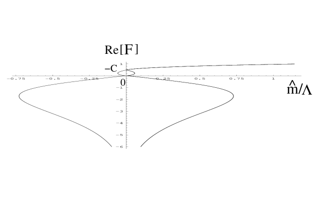
Figure 3: The different branches of $F$ at second RG order in Eq. (8) in the $O(2N)$ GN ($N=2$).

Similarly to first RG order in Eq. (18), $F$ has a power expansion for sufficiently small $\hat{m}$: defining

$$F(x)\equiv A\>G[\>\frac{C^{(B-C)/A}}{A}\>x^{1/A}]$$ (22)

with $x=\hat{m}/\Lambda$, one has from (8)

$$G=x\;e^{-G}(1+\frac{A}{C}\>G)^{C-B}\equiv x\;[1+\sum^{\infty}_{p=1}a_{p}x^{p}]$$ (23)

where the expansion coefficients $a_{p}$ are now more involved than the first order corresponding ones in (18) (the $a_{p}$ will now depend explicitly on the RG quantities $A$, $B$, $C$), but can be derived systematically . It is easy to determine the convergence radius of this expansion form of $F(\hat{m})$ around zero, given by the location of its closest non-zero singularity:

$$\frac{d\,\hat{m}}{dF}(F^{*})=0\to F^{*}=-\frac{1}{2}\;(\frac{\gamma_{0}}{2b_{0}})\;[1\pm\sqrt{1-4\frac{\gamma_{1}}{\gamma^{2}_{0}}}\;\;]\;,$$ (24)

and correspondingly

$$\frac{\hat{m}^{*}}{\Lambda}=e^{F^{*}}(F^{*})^{A}(C+F^{*})^{(B-C)}$$ (25)

so that $R_{c}\equiv|m^{*}/\Lambda|$. Note that for $N\to\infty$, $F^{*}=-1$ and correspondingly $\hat{m}^{*}/\Lambda=-e^{-1}$. This is due to the fact that for $N\to\infty$ $F$ is exactly the Lambert function, see Fig. 1. At second RG order, in the $O(2N)$ GN model, $F^{*}<0$ and $C+F^{*}<0$ are real and negative $\forall N\geq 3/2$, so that the number and location of the singularities in Eq. (25) on the circle of radius $R_{c}$ are determined by the roots of $(-1)^{A+B-C}$, see Fig. 4.

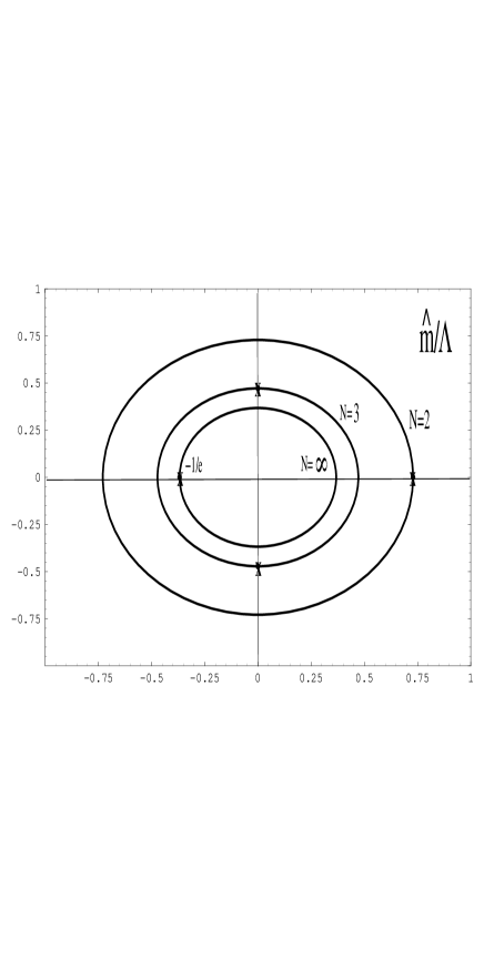
Figure 4: Convergence radii of the power expansion form Eq. (23) of $F$ at second RG order, Eq. (8), and corresponding singularity locations on the convergence circle for different values of $N$ in the $O(2N)$ GN model.

II.2 Other renormalization schemes

Before to proceed we should remark that at second RG order there is a certain arbitrariness in e.g. Eq. (8) and related quantities, like (24)–(25), since $\gamma_{1}$ is renormalization scheme (RS)-dependent: more precisely, for an arbitrary perturbative RS change in the Lagrangian mass and coupling parameters:

$$g^{2}\to\tilde{g}^{2}=g^{2}\;(1+A_{1}g^{2}+\cdots)\;,$$

$$m\to\tilde{m}=m\;(1+B_{1}g^{2}+\cdots)\;,$$ (26)

$\gamma_{1}$ is changed as

$$\tilde{\gamma}_{1}=\gamma_{1}+2b_{0}B_{1}-\gamma_{0}A_{1}\;\equiv\;\gamma_{1}+\delta\gamma_{1}\;,$$ (27)

while $b_{0}$, $b_{1}$ and $\gamma_{0}$ are RS-invariant, as already mentioned (more details on RS changes are given in Appendix C). This means for instance that the location of the singularities and the value of the convergence radius as implied by (25) may be modified, to some extent, by appropriate changes in $\gamma_{1}$ (equivalently changes in the quantity $A\equiv\gamma_{1}/(2b_{1})$ as defined in (11)).
It is always possible to choose the ‘t Hooft scheme, in which Eqs. (6), (9), (8) resum the complete RG dependence in $\hat{m}$. This is convenient because beyond second RG order, in an arbitrary scheme where $b_{i},\gamma_{i}\neq 0$ for $i\geq 2$, algebra becomes quite involved, and neither the non-log contributions $d_{n}$ nor the $b_{n}$ and $\gamma_{n}$ RG coefficients are known at arbitrary orders for most field theories, and in particular for the GN model. Nevertheless it is still possible to work out a formal generalization of Eq. (6), in an arbitrary (MS) scheme, see Appendix A. We will use this generalization to define some of the numerical approximations to the mass gap, of arbitrary higher orders, in section VII.
Before to conclude this section, we discuss another possible RS choice, obtained from expression (6) by an all orders redefinition of $F$:

$$F\equiv\tilde{F}-(A+B-C)\ln\frac{F}{\tilde{F}}-(B-C)\ln[1+\frac{C}{F}]$$ (28)

which can be perturbatively expanded in powers of $1/\tilde{F}$, where $\tilde{F}$ is now again directly related to the Lambert function:

$$\tilde{F}(\frac{\hat{m}}{\Lambda})\equiv\ln[\frac{\hat{m}}{\Lambda}]-(A+B-C)\ln\tilde{F}\;\equiv\tilde{A}W[(\frac{\hat{m}}{\Lambda})^{1/\tilde{A}}/\tilde{A}]$$ (29)

with $\tilde{A}\equiv A+B-C$. This redefinition is motivated from the fact that in the GN model, the RG coefficient $C<0$ in Eq.(11), due to $b^{GN}_{1}<0$, which corresponds to an infrared fixed point at $g_{c}=-b_{0}/b_{1}>0$, so that the perturbative branch of $F$ reaches $\hat{m}\to 0$ first for $F=-C$. In the scheme (28), Eq. (6) takes the form:

$$M^{P}(\hat{m})=(2/e)^{-C}\>\hat{m}\;\tilde{F}^{-(A+B)}\;\sum^{\infty}_{n=0}\tilde{d}_{n}\>(2b_{0}\tilde{F})^{-n}\;.$$ (30)

This also implies appropriate changes in the purely perturbative coefficients, simply determined by re-expanding Eq. (8) in $1/\tilde{F}$ powers:

$$\tilde{d}_{1}=d_{1}-B\;C\;,\;\;\cdots$$ (31)

III Infrared renormalon properties of the GN pole mass

As mentioned in introduction, the idea is that, since the complete pole mass Eq. (6) gives the ratio $M^{P}(F)/\Lambda$ to all perturbative orders for $\hat{m}\gg\Lambda$, if we are able to resum this series and to give it a meaning for $\hat{m}\to 0$, we can obtain the $M^{P}/\Lambda$ ratio in the physically interesting massless limit. As far as the pure RG dependence is concerned, this turns out to be possible because $F(\hat{m})$ provides a rigorously defined and explicit bridge between the “non-perturbative” $\hat{m}\raisebox{-3.69899pt}{~{}\shortstack{$<$ \\ [-0.07cm] $\sim$}}~{}\Lambda$ regime, where $F$ has power expansion (18), and the short distance perturbative $\hat{m}\gg\Lambda$ (logarithmic) regime. A crucial point indeed is the difference between the usual effective coupling $g^{2}(p^{2})\equiv 1/[b_{0}\>\ln(p^{2}/\Lambda^{2})]$, having a Landau pole at $p^{2}=\Lambda^{2}$, and $F^{-1}(\hat{m})$ here, having its pole at $\hat{m}=0$, governing the massless limit (19) of the (pure RG) mass gap Eq. (9). Accordingly along the continuous branch on Fig. 2, $M(\hat{m})$ has no singularity for $0<\hat{m}<\infty$, as is clear also from Eq. (19) and Fig. 1, 2. Now, to extrapolate the complete pole mass (6) down to the chiral, strongly coupled regime $\hat{m}\simeq 0$, the main obstacle comes from the presence of the purely perturbative coefficients $d_{n}$. First, though the pole mass (or other physical quantities similarly) is infrared finite, gauge Tarrach –, scale– and scheme–invariant, the relation between the pole mass and e.g. the running mass in (14) is scheme dependent, which is manifested here by the RS-dependence in (6) of the perturbative coefficients $d_{n}$, the RG coefficients $A$, $B$ in Eq. (11), and of $\Lambda$ too.
Second, it is immediate that the perturbative contributions $d_{n}/F^{n}$ in Eq. (6) are singular when $F\to 0$ ($\hat{m}\to 0$), since each term will have a leading divergence $\simeq d_{n}\;(\hat{m}/\Lambda)^{-n/A}$, according to (18). In other words, while the usual Landau pole problem was avoided in the pure RG part (9) of $M^{P}$, which has a regular finite $\hat{m}\to 0$ limit, as illustrated in Figs. 1–3, a problem reappears in the perturbative corrections relating the true physical quantities, like the pole mass, to their pure RG part. Thus, in an arbitrary scheme, strictly speaking $M^{P}\to\infty$ when $\hat{m}\to 0$. (In principle one could avoid this problem in a crude way by exploiting the RS arbitrariness in (6) to define a scheme such that all the perturbative coefficients $\tilde{d}_{n}\equiv 0$. Although such a peculiar scheme can always be formally constructed, this solution is to be considered unsatisfactory, since one expects truly non-perturbative results not to depend on a particular scheme.) This appears in fact completely similar to the perturbative expansion in powers of $(g/m^{3})$ of the oscillator energy levels, thus also singular for $m\to 0$, which nevertheless do not prevent different resummation methods to work very wellao ,delta –deltac , even for $m\to 0$. We will see in next sections how similar resummation properties generalize, to some extent, in the present field theory case.

Figure 5: The GN mass graphs at order $1/N$.

Now there is unfortunately an even worse problem, when dealing with the purely perturbative expansion of the pole mass: in the $O(N)$ GN model, at order $1/N$, it exhibits infrared renormalons very similar to the QCD quark pole massMPren ; renormalons . More precisely, let us consider only the naive perturbative expansion of the pole mass, obtained from Fig. 5 by taking perturbative expression of the dressed scalar propagator (wavy line), $G^{-1}(q^{2})\sim g^{2}(q^{2})\sim[b_{0}\>\ln(q^{2}/\Lambda^{2})]^{-1}$:

$$M^{P}=1+\frac{1}{4N}\int^{\mu^{2}}_{0}\frac{dq^{2}}{M^{2}}(1-\zeta)\;\left[g^{2}(q^{2})-{\cal O}(\frac{M^{2}}{q^{2}})\right]$$ (1)

where $\zeta=(1+4M^{2}/q^{2})^{1/2}$ and $M\equiv\mu e^{-1/(2b_{0}\>g^{2}(\mu))}$ is the mass gap at leading $1/N$ order. Then a standard calculation givesKRcancel

$$d_{n+1}\raisebox{-11.38092pt}{~{}\shortstack{ $\sim$ \\ $n\to\infty$}}(2b_{0})^{n}\>n!$$ (2)

so that the series Eq. (6) including this next-to-leading $1/N$ order is badly divergent for any $\hat{m}$, and not even Borel summable: such a factorial growth of the perturbative coefficients, with no sign alternation, impliesrenormalons ambiguities of ${\cal O}(\Lambda)$. But, those renormalons are only perturbative artifacts: considering now the full scalar propagator contribution (which is known exactly for the $O(N)$ GN model at $1/N$ order):

$$G[q^{2}]=\left[1+\frac{g^{2}\,N}{2\pi}\left[\ln\frac{M^{2}_{P}}{\mu^{2}}+\zeta\ln[\frac{\zeta+1}{\zeta-1}]\>\right]\right]^{-1}=\left[\frac{g^{2}\,N}{2\pi}\zeta\ln[\frac{\zeta+1}{\zeta-1}]\right]^{-1}+{\cal O}(1/N)\;,$$ (3)

rather than its truncated perturbative contribution Eq. (1), the exact $1/N$ expression of the pole mass is obtainedKRcancel ; FNW as

$$M^{P}=\Lambda\left[1+\frac{1}{2N}[Ei[-\theta]-\ln\theta-\gamma_{E}+\ln(\ln\frac{\mu^{2}}{M^{2}})-2\ln(\cosh[\theta/2])+\ln\frac{\mu^{2}}{M^{2}}\;]\right]$$ (4)

with $\chi=(1+4M^{2}/\mu^{2})^{1/2}\equiv 1/\tanh(\theta/2)$ (i.e. $\theta=\ln[(\chi+1)/(\chi-1)]\;\geq 0$), and $Ei(-x)\equiv-\int^{\infty}_{x}dte^{-t}/t$ the Exponential Integral function ($x\geq 0$). Thus $Ei[-\theta]$ has a factorial perturbative series with sign-alternated coefficients, i.e. the IR renormalons actually disappear: more precisely we can re-expand the result (4) in perturbation, using

$$\ln[\frac{\chi+1}{\chi-1}]\simeq\ln\frac{\mu^{2}}{M^{2}}+2\frac{M^{2}}{\mu^{2}}+\cdots=g^{-2}+2\frac{M^{2}}{\mu^{2}}+\cdots$$ (5)

$$M^{P}=M\left[1+\frac{1}{2N}\left(2\ln 2-\gamma_{E}-\frac{M^{2}}{\mu^{2}}[\sum^{\infty}_{n=0}(-1)^{n}n!\;g^{2(n+1)}\;+{\cal O}(\frac{M^{2}}{\mu^{2}})]\right)\right]$$ (6)

The explicit Borel summability of the genuine perturbative expansion, Eq.(6), is not in contradiction with the purely perturbative results above, because the non-trivial cancellation of renormalons involve the contributions of non-perturbative power corrections contributionsKRcancel ; David ; Benbraki . Moreover, it turns out that this cancellation is such that the final expression of the pole mass contains neither “purely perturbative” nor “intrinsically non-perturbative” contributions: for instance, the net contribution due to the first graph in Fig. 5 is the term $-\gamma_{E}$ in Eq. (6), which simply remains after cancellation of the first order terms:

$$-\int_{0}^{\infty}dt\left[\frac{1}{t(1+t)}+e^{-t/g^{2}}[-\frac{1}{t}+{\cal O}(\frac{M^{2}}{\mu^{2}})\>]\right]$$ (7)

$$\sim -\frac{1}{2}[\gamma_{E}+{\cal O}(\frac{M^{2}}{\mu^{2}})]$$

Now, the point is that the above results Eqs. (4), (6) obviously could only be obtained from calculating explicitly the exact mass gap at next-to-leading $1/N$ order. Our aim here is to ignore on purpose these exact $1/N$ results, a priori only accessible in a certain class of 2-D models. Rather, we want to examine whether our generic construction, relying solely on the purely perturbative information, together with the infrared properties of the function $F$, is able to recover some of the non-perturbative properties of the exact mass gap, in particular its Borel summable asymptotic expansion explicit at next-to-leading $1/N$ order.

IV Borel summability of the $F$ expansion

We first reexamine here why the expression (6) is plagued with perturbative ambiguities, and how one can get rid of those, within our construction, thanks to the analytic properties of $F$ in a vicinity of $\hat{m}=0$ valuesKRlet . First we define from Eq. (6) its Borel transformed series:

$$B.T.[M^{P}(F)](t)\equiv 2^{-C}\hat{m}\>F^{-A}(C+F)^{-B}\;\left[1+\sum^{\infty}_{n=1}\frac{d_{n}\>t^{n}}{(n-1)!}\right]$$ (8)

so that the corresponding Borel integral reads:

$$BI(\hat{m})\equiv\tilde{M}^{P}(\hat{m})=2^{-C}\hat{m}\>F^{-A}(C+F)^{-B}\int^{\infty}_{0}\!dte^{-t}\;[1+(4\pi\,b_{0}\,F)^{-1}\sum^{\infty}_{n=0}(\frac{t}{F})^{n}\>]$$ (9)

upon assuming for the perturbative coefficients $d_{n}$ the leading large order behaviour in Eq. (2). For any $F>0$, this expression would be (asymptotically) equal to (6) by formal expansion, would the pole at $t=F$ not make the integral (9) ill-defined. One should make a choice in e.g. deforming the contour above (or below) the pole, which results in an ambiguity, which is easily seen to be proportional to ${\cal O}(e^{-F})$. Since from Eq. (15) $F\sim\ln[\hat{m}/\Lambda]-A\ln[\ln[\hat{m}/\Lambda]]$ for $\hat{m}\gg\Lambda$, this implies a perturbative ${\cal O}(\Lambda/m)$ ambiguity for the “short distance” ($M,\hat{m}\gg\Lambda$) pole mass:

$$\mbox{ambig}\;\sim\pm i\;(\frac{\Lambda}{\hat{m}})\;\ln^{A}[\frac{\hat{m}}{\Lambda}]\;,$$ (10)

in consistency with general resultsrenormalons . Now in our case, Eq. (17) (and equivalently Eqs.(22),(23) at second RG order) allow to trace the behaviour of $F$ all the way down to $\hat{m}\to 0^{+}$, where at first RG order, $F\to 0$: consequently the naive mass gap (6), expected to be $\sim\Lambda$, is also ambiguous by ${\cal O}(\Lambda)$.
But in contrast, within our construction, the Borel integral (9) can be defined unambiguously and independently of the RS parameter $A$, in the range $F<0$KRlet : then $F\equiv-|F|$ simply produces the adequate sign alternation in the factorially growing coefficients $\sim F^{-n}$. More precisely, a straightforward calculation of Eq. (9) for $Re[F]<0$ (neglecting for simplicity at the moment the two-loop RG dependence $C$, irrelevant to asymptotic properties), gives

$$BI(\tilde{M}^{P}/\Lambda)\raisebox{-11.38092pt}{~{}\shortstack{ $\sim$ \\ $F<0$}}e^{-|F|}+\frac{1}{2b_{0}}\>Ei(-|F|)$$ (11)

where we also used Eq. (20) to express $M^{P}/\Lambda$ as a function of $F$ only. Indeed, as already mentioned the first RG order function $F(\hat{m})$ in (15) is well-defined (analytic) for any $A$ values in a disc of radius $e^{-A}A^{A}$ around zero (and for $A=1$ the only singularity is at $F=-1$ i.e. $\hat{m}/\Lambda=-e^{-1}$, cf. Fig. 1). Thus, one can choose the branch of $F$ such that $Re[F(\hat{m})]<0$, compatible with the limit $\hat{m}\to 0$. The second RG order $F$ in Eq. (8) has similar properties, with finite convergence domain around $F=0$ and $F=-C$ respectively, see Fig 3 . More generally, in an arbitrary AFT with arbitrary values of the RG parameters $A$, $B$, $C$ depending on the renormalization scheme, there always exist branches of $F$ such that $F$ is complex. This is the case for the GN model for the two branches shown with $Re[F]<-C$ in Fig. 3. As a consequence, the Borel singularities in e.g. Eq. (9) are moved away from the real semi-axis of Borel integration $Re[t]>0$, now being located at $t_{0}=F\equiv|F]e^{i\theta_{F}}$ with $\theta_{F}\neq 0$.

We obtain in this way formal Borel convergence for a certain range of the expansion parameter near the relevant massless limit $\hat{m}=0$, strictly only along those branches such that $F<0$, or more generally complex. Depending on the branch of $F$, this may correspond either to $\hat{m}>0$ or $\hat{m}<0$ (see Figs. 2,3), which is in principle not a problem, since relativistic field theories only depend on $m^{2}$ (the sign of the Lagrangian mass term in (1) can be flipped by a discrete $\gamma_{5}$ transformation, and the Dirac equation is invariant under $m\to-m$). In Fig. 2, the complex branches of $F$ are those corresponding to $Re[M]/\Lambda<1$, and to $Re[F]<-C$ in Fig. 3, where in both cases the symmetry with respect to $\hat{m}\to-\hat{m}$ of such pure RG dependence is manifest. More generally, we expect that our final, physical mass gap result, should be independent of the way in which the massless limit is to be reached, either from $Re[F]>0$, or $Re[F]<0$, or more generally from any of the complex branches of $F$. However, the (unphysical) perturbative expansion is clearly not invariant under this, since the (usual) expansion with real $F>0$ is non Borel summable and ambiguous. Therefore, the following picture emerges: in our construction, the perturbative expansion near the strongly coupled, massless limit can exist in two modes:
i) in the standard mode, corresponding to real $F>0$, and matching the usual perturbative expansion for $\hat{m}\gg\Lambda$, the perturbative expansion alone has to be necessarily completed as usual with “non-perturbative” power corrections, as illustrated explicitly with the exact $1/N$ calculation of the GN mass gap, discussed in section 3.
ii) In the “alternative” expansion mode, with $F<0$ in the simplest case (first RG order) where $A_{0}=1$, the perturbative series is directly Borel summable, thus non-ambiguous. There is, therefore, no explicit non-perturbative power correction contributions needed in principle. Those results are completelly general for a renormalizable AFT of dimension $D\geq 2$, since they only depend on the generic RG properties of the function $F$.
To illustrate perhaps better the last points, we can give an analogy, to some extent, in the simplest possible model where such issues can be discussed, the anharmonic oscillator. The detailed analogy is discussed in Appendix B. The oscillator is describedao by a $g\phi^{4}$ massive scalar field theory in 1-D, with energy levels having from purely dimensional considerations a perturbative expansion in powers of $g/|m|^{3}$:

$$E_{0}\sim|m|\;\sum_{n}a_{n}(\frac{g}{|m|^{3}})^{n}\;,$$ (12)

with factorially growing but sign-alternated coefficientsao ; zinn : $a_{n}\sim(-1)^{n}n!$ at large orders, thus the energy levels are Borel-summableaoBsum . Now, let us assume, momentarily, that our only knowledge of the oscillator would consist of the perturbative expansion Eq. (12), and consider formally changing the sign of the coupling $g$ there: this obviously induces a change of sign in the perturbative coefficients, rendering the corresponding series non Borel summable . This accordingly produces an ambiguity, an imaginary part in the energy, whose leading terms can be evaluated exactly still using the Borel integral, and according to the standard interpretation it calls for additional non-perturbative corrections. The latter are easily shown to have the form of the standard instanton contributions to the ground-state energyzinn :

$$Im\,E_{0}\sim\frac{4}{\sqrt{2\pi}}\;e^{\frac{4m^{3}}{3g}}\;(\frac{m^{3}}{-g})^{1/2}$$ (13)

where $g<0$, and governing accordingly the decay of the wave function due to barrier penetration zinn (see appendix B for more details). Of course, this instanton contribution was originally not derived from the perturbative ambiguity, since in the oscillator case a “direct” non perturbative calculation is possible. But as seen from the “perturbative only” side, the above argument indicates that, already for the simpler oscillator case, the perturbative expansion can exist in two different modes, one in which it is directly Borel summable, while for $g<0$ non-trivial non-perturbative contributions are needed to get a consistent physical picture.

Coming back to the $D\geq 2$ field theory case, we stress, however, that the above discussed Borel summability properties in our construction is possible due to the negative (more generally complex) tail of the perturbative expansion parameter $1/F$ in the infrared, rather than due to an artificial change of sign for any $F$ values. One may wonder if such a sign alternation of the badly behaving infrared factorials, may not alter the other way round the signs of the UV renormalons, which originally have the good (alternated) signs in AFTrenormalons . It is easily realized that they are in fact unaffected by the infrared properties of $F<0$, since by definition the UV renormalons originate only from the domain $\mu\gg\Lambda$ (more precisely the Borel integral equivalent to Eq. (9) for UV renormalons corresponds to integration from $\mu^{2}<q^{2}<\infty$). In this range, $F$ is necessarily real positive and large, see Fig. 1 and Fig. 3.
Remark finally that, only from the properties of $F$ around $F\raisebox{-3.69899pt}{~{}\shortstack{$<$ \\ [-0.07cm] $\sim$}}~{}0$, the Borel sum in (11) reproduces qualitatively the asymptotic behaviour of the exact $1/N$ result Eq. (4) in the $O(N)$ GN model (with $4\pi b_{0}=2N-2$), except for finite terms $\gamma_{E}$ etc, which not surprisingly cannot be guessed by our simple Borel summation of the (leading) renormalon asymptotic behaviour in Eq. (9), and with only the first order RG dependence included. Thus, at this stage the Borel summability property of the series for $F<0$ plays a rather formal role, since the leading order Borel sum Eq. (11) is not expected to be a good numerical approximation of the exact mass gap. (We shall see in section VII that there are more efficient approximations to the exact mass gap.)

It is not difficult to work out the exact second RG order generalization of Eq. (11). For this purpose, it is convenient to define another change of scheme, by a “non-perturbative” redefinition of $F$:

$$F+C\equiv f$$ (14)

perturbatively equivalent to

$$g^{2}\to\tilde{g}^{2}=g^{2}\;(1+\frac{b_{1}}{b_{0}}g^{2})^{-1}\;.$$ (15)

This redefinition is again motivated from the fact that in the GN model, the RG coefficient $C<0$ in Eq.(11), so that the extrapolation from the perturbative range of (9) down to $\hat{m}\to 0$ reaches first $F=-C$, as explained before(see Fig. 3). The asymptotic behaviour of the perturbative coefficient (exact in the scheme (2)) is

$$d_{n+1}\raisebox{-11.38092pt}{~{}\shortstack{ $\sim$ \\ $n\to\infty$}}(2b_{0})^{n}\>\Gamma[n+1+C]\;$$ (16)

for $n\to\infty$. The corresponding Borel integral reads

$$BI(M^{P})[f]=\Lambda\;(2e)^{-C}e^{f}f^{-C}\;[1+\frac{\Gamma[1+C]}{4\pi b_{0}\,f}\int^{\infty}_{0}\!dte^{-t}\;(1-t/f)^{-1-C}\>]$$ (17)

where we used the appropriate RS change Eq. (14) in Eq (6). So for $F<-C$, i.e. $f<0$, we obtain

$$BI(M^{P})[-|f|]\sim\Lambda\;(2e)^{-C}e^{-|f|}(-|f|)^{-C}\;[1-\frac{1}{4\pi\,b_{0}}\>\Gamma[1+C]\>e^{|f|}\>|f|^{C}\>\Gamma[-C,|f|]\>]$$ (18)

where the $1$ in the bracket refers to the pure RG part, while the remaining part in Eq. (18) resums the purely perturbative contributions. The latter resummation of the perturbative expansion part is convergent, giving a finite contribution $\forall|f|\neq\infty$. In particular it gives a finite result even for $|f|\to 0$:

$$\mbox{BI[pert. series]}\raisebox{-11.38092pt}{~{}\shortstack{ $\to$ \\ $|f|\to 0$}}-(-1)^{-C}\>(2e)^{-C}\>\frac{1}{4\pi\,b_{0}}\>\Gamma[1+C]\>\Gamma[-C]$$ (19)

which accordingly, corresponds to reach the massless limit $\hat{m}\to 0$ along any of the branch of $F$ below $F=-C$, see Fig. 3. Remark also finally that Eqs. (18), (19) only depend on the universal RG coefficient $C$ in (11) (noting also that $4\pi b_{0}=-C^{-1}=2N-2$ in the GN model).

V Variationally improved mass expansion

We examine now how to complement the above construction, based only on RG fixed point properties, by combining it with a specific variant of the delta-expansion, or variationally improved perturbation (DE-VIP) method. The latter is usuallypms ; delta applied more directly on the ordinary perturbative series in the coupling $g$. But the present construction and the DE-VIP idea are closely related, the DE-VIP being essentially a reorganization of the interaction terms of the Lagrangian, with the introduction of a trial mass parameter, for physical quantities relevant in the massless limit of the theory. We will see that the DE-VIP can give further improved Borel convergence properties. We define the (linear) DE as the power series obtained formally after the substitution

$$m(\mu)\to(1-\delta)\;m_{v};\;g^{2}(\mu)\to\delta\>g^{2}(\mu)$$ (1)

within any perturbative expressions at arbitrary order, where $m(\mu)$ is the renormalized Lagrangian mass (in e.g. $\overline{\small{MS}}$ scheme), $\delta$ the new expansion parameter, and $m_{v}$ an arbitrary adjustable mass. (1) is equivalent to adding and subtracting to the massless Lagrangian a “trial” mass term $m_{v}$ [$\delta$ interpolating between the free ($\delta=0$) and the interacting massless Lagrangian ($\delta=1$)], and is entirely compatible with renormalizationgn2 and gauge-invarianceqcd2 . After substitution (1),

$$M^{P}(\hat{m},\delta)\equiv\sum_{k}a_{k}(\hat{m})\delta^{k}$$ (2)

can be most conveniently directly resummed, for $\delta\to 1$, by contour integrationgn2 around $\delta=0$, to arbitrary order $K$: an appropriate change of variable allowing to study the $m(\mu)\to 0$ (equivalently $\delta\to 1$) limit in Eq. (1) is:

$$\delta\equiv 1-v/K\;;\;\;\;m_{v}=K^{\gamma}\;\hat{m}_{v}\;.$$ (3)

Eq. (3) is simply a convenient way of parameterizing how rapidly the Lagrangian mass $m(\mu)\to 0$ limit is reached (as controlled by $\gamma\leq 1$) as function of the (maximal) delta-expansion order $K$. Similarly to refs. deltaconv ; deltac the point is to adjust the rates at which $m(\mu)\to 0$ ($\delta\to 1$) and $K\to\infty$ are simultaneously reached, with no a priori need of invoking explicit PMS optimization principle. The final contour integral summation takes a simple form, for $K\to\infty$:

$$\frac{M^{P}}{\Lambda}\sim 2^{-C}\frac{1}{2\pi i}\oint dv\;e^{(v/m^{\prime\prime})}\;F^{-A}[v]\>(C+F[v])^{-B}[1+\frac{1}{2b_{0}\,F[v]}\sum^{N}_{n=0}\frac{d_{n}}{F^{n}[v]}]$$ (4)

where $m^{\prime\prime}\equiv\hat{m}_{v}/\Lambda$, $N$ is the maximal perturbative order, and after a deformation the contour encircles the semi-axis $Re[v]<0$ (see Fig. 6).

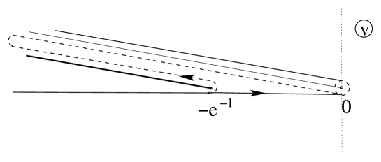
Figure 6: Singularities and equivalent integration contours in the $v$ plane, for $A=1$.

For simplicity we fix from now the scaling parameter in Eq. (3) to its maximal value ($\gamma=1$) still compatible with massless limit (i.e. $m_{v}\to 0$). (NB The general $\gamma$ scaling (3) can be analyzed in a way more similar to the oscillator deltaconv ; deltac , i.e. without the peculiar contour $\delta$-summation Eq. (4), see Appendix D. But this gives rather cumbersome algebraic and numerical analysis.) Eq. (4) can be well approximated analytically (at least for slightly restricted RS choices, as will be indicated):

$$M^{P}/\Lambda\sim 1+\frac{1}{4\pi b_{0}}\;\sum^{N}_{q=1}\left[\;\sum^{N-q}_{p=0}\frac{\Gamma[p+q](p+q+A)(q+A)^{p-1}}{A^{p}\>\Gamma[1+p]\>\Gamma[1+q/A]}\;\right](m^{\prime\prime})^{-q/A}$$ (5)

where we used Eq. (18), leading to the (exact) expression

$$F^{-n-A}(m_{v}\;v)=\sum^{\infty}_{p=0}\frac{(n+A)(n+A-p)^{p-1}}{p!\;A^{p}}(m_{v}\;v)^{-1+\frac{p-n}{A}}$$ (6)

together with

$$\frac{1}{2\pi\,i}\oint dve^{v}v^{z}=\frac{1}{\Gamma[-z]}\;,$$ (7)

and also assumed the leading renormalon behaviour Eq. (2). In Eq. (5) we also made a convenient reshuffling of summation indices, $n\to p+q$, where $n$ is the original perturbation order, $p$ is the order of the expansion in Eq. (18), and $q$ is the order of the (resulting) expansion in $(m^{\prime\prime})^{-q/A}$.
In fact, some restrictions applyKRlet to Eq. (5): the sum over $p$ is bounded as given, iff

$$1/A\in\mathbf{N}^{*}\;,$$ (8)

since $1/\Gamma[1+(n-p)/A]=0$ for $p\geq n+1$, which we assume in this section for simplicity. (This is not much restrictive, except that for arbitrary AFT it is generally not possible both that $A$ satisfies (8) and $B=0$ in Eq. (11), as assumed in (4). But the more general scheme $B\neq 0$ simply makes Eq. (5) algebraically more involved, without affecting the large order behaviour and convergence properties.)
Second, strictly (5) is valid only asymptotically, for sufficiently large $N$: due to the finite convergence radius of expansion (18), interchanging the sum in (18) and integration in (4) is not rigorously justified. However, when (8) holds, the formerly branch point $v=0$ is simply a pole, which allows to choose an equivalent contour of arbitrarily small radius around $v=0$, thus always inside the convergence radius of (18) (see the dashed small circle contour in Fig. 3). Using Eq. (6) (exact for $|m_{v}\;v|<e^{-A}A^{A}$); and $e^{v}=\sum_{k}v^{k}/k!$, it is easily seen that the simple poles are for

$$k-(1+(n-p)/A)=-1$$ (9)

for which the contribution to the contour integral will be the coefficient (6), divided by $k!$: this give $\Gamma[1+(n-p)/A]=\Gamma[1+q/A]$. So, only the simple pole terms $v^{-1}$ contribute to Eq. (4), which sum up to give Eq. (5) again. The extra contribution (around the cut at $v=-e^{-1}$, e.g. for $A=1$) gives the difference between the “exact” integral (4) and expansion (5), and can be evaluated numerically. These contributions are easily shown for $A=1$ to contribute as ${\cal O}(e^{-(e\>m^{\prime\prime})^{-1}})h[N]$ relative to (5), where $h[N]$ rapidly decreases for $N\to\infty$. In Table 1 we compare, for the first 20 values of the perturbative order $n$, and for $m^{\prime\prime}=1$, the exact integrals:

$$I^{exact}_{n}=\frac{1}{2\pi\,i}\oint dve^{v/m^{\prime\prime}}F^{-n-A}[v]$$ (10)

which we calculated numerically with Mathematicamatha , with the approximation using the expansion (6) (thus neglecting the extra contribution around $-e^{-1}$):

$$I^{series}_{n}=\sum^{n}_{p=0}\frac{(n+A)(n+A-p)^{p-1}}{p!\;A^{p}\>\Gamma[1+(n-p)/A]}(m_{v})^{-1+(p-n)/A}$$ (11)

that leads to Eq. (5). We also give in the third column of Table 1 the extra $e^{-1}$ cut contribution, evaluated independently numerically for consistency.

n	$I^{exact}_{n}(m^{\prime\prime}=1)$	$I^{series}_{n}(m^{\prime\prime}=1)$	-$e^{-1}$ cut contribution
0	1.137545624095354	1.	0.1375456240953545
2	4.992495983527079	5.	-0.00750401647292076
4	8.165946096293188	8.166666666666666	-0.0007205703734776136
6	8.780755015889008	8.780555555555555	0.0001994603334534161
8	7.28191740833204	7.281944444444444	-0.00002703611240395531
10	5.01821660133935	5.0182137345679	2.86677144956 10-6
12	2.99921746894628	2.999217731214259	-2.62267978889 10-7
14	1.597938546376994	1.597938525158887	2.121810749323 10-8
16	0.773538637086908	0.773538638583302	-1.4963940087 10-9
18	0.3450035964997671	0.3450035964141139	8.5653262261 10-11
20	0.1432800076663147	0.1432800076691064	-2.79173906215 10-12

Table 1: Comparison between Eq. (10) (evaluated numerically), Eq. (11), and the extra cut contributions.

When $m^{\prime\prime}\to 0$, the discrepancy between the exact integral and the analytical resummation in Table 1 decreases rapidly, as expected, even for small $n\to 0$ (but the numerical integration becomes unstable for very small $m^{\prime\prime}$). If $A\neq 1$ and $B$ arbitrary, contributions from extra cuts are not so simply estimated, and we were only able to check numerically that they are negligible with respect to (5) for sufficiently large $N$.] Thus for large enough $N$ (and/or small $m^{\prime\prime}$) those contributions are unessential for the convergence properties discussed below.

The factorial damping of coefficients, as compared to the original perturbative expansion, is explicit in Eq. (5). Yet, the damping is insufficient to make this series for $N\to\infty$ readily convergent. For any low $p\ll N$, renormalon factorials are overcompensated if $A\leq 1$, but the $\Gamma[1+q/A]$ damping decreases in strength as $p$ increases, giving increasing contributions to the sum over $p$. The leading contributions to the coefficients of (5) happen at intermediate values of $p$. Nevertheless, the idea of damping factorials from appropriate RS choice does survive, when considering the Borel transform of Eq. (5), as examined next.

VI Borel convergence of DE-VIP

We are now ready to combine the previous DE-VIP behaviour of the series in $\hat{m}/\Lambda$ with the general Borel convergence properties for $Re[F]<0$ of the initial perturbative series in $1/F$, which were examined in section 4. For completeness we consider both a linear and non-linear version of the DE-VIP construction, also for reasons that will be clear below. We will see that the DE-VIP expansion can generally improve (accelerate) the Borel convergence properties of the $1/F$ expansion.

VI.1 Linear method

For any given choice of contour avoiding the pole in the Borel plane $t$ (or cut at higher RG order, see Eq. (17)), we can apply the DE-VIP as defined in section 4, introducing the $\delta$–expansion and contour resummation as in Eq. (4), but now on the Borel integral Eq. (9) (or Eq. (17)). It leads to:

$$\tilde{M}^{P}_{var}(\hat{m}_{v})\sim\frac{2^{-C}}{2i\pi}\oint dve^{v}\;\frac{\hat{m}_{v}}{F^{A}\,(C+F)^{B}}\;\int^{\infty}_{0}dte^{-t}\;[1+\frac{1}{4\pi\,b_{0}\,F}(1-t/F)^{-1}\>]$$ (1)

where $F\equiv F[\hat{m}\>v]$ and the integrand is to be be understood as its formal expansion in $t/F[\hat{m}\>v]$. Interchanging the contour and Borel integrals, the Borel transform integrand, which is a function of $t$, is essentially Eq. (5) but with the replacement

$$\Gamma[p+q]\to t^{p+q}$$ (2)

standard from the Borel transform, except that in our case we did some reshuffling of summation indices, as already indicated after Eq. (5). One can find after some algebra the asymptotic behaviour for (the original maximal perturbative order) $N\to\infty$:

$$\tilde{M}^{P}_{var}(m^{\prime\prime})\sim const.\;\Lambda\;[1+\int^{\infty}_{0}\!\frac{dt}{4\pi\,b_{0}}\,\,\sum^{\infty}_{q}\frac{(t^{A}e^{t}/m^{\prime\prime})^{q/A}}{\Gamma[1+q/A]}\;]$$ (3)

where we work again here for simplicity at first RG order, neglecting the pure RG resummed $(C+F)^{-B}$ term in (9). It thus appears that the asymptotic behaviour of the Borel integrand in Eq. (3) is that of an entire series (at least for $A>0$), i.e. with no poles for $0<t<\infty$. More precisely, the pole at $t_{0}=1$ in the original (standard) Borel integrand has been pushed to $t_{0}\to+\infty$ due to the factorial damping, so that the Borel integral is no longer ambiguous. However, integral (3) is badly divergent at $t\to\infty$, at least for $Re[m^{\prime\prime}]>0$, so that the series is not Borel summable for standard (perturbative) $m^{\prime\prime}$ values. In fact it is important to remark that this non convergent result is obtained when considering the exact expansion of $F$, Eq. (18), to all orders. Naively, one may have thought that the contour integral would be dominated for $q\sim N\gg p$, by the apparently ”leading” terms for $m^{\prime\prime}v\simeq 0$ in Eq.(4). But the asymptotic behaviour of our complete series Eq.(5), as well as its Borel transform Eq. (3), appear much less intuitive than e.g. the oscillator energy levels expansions. Therefore, it is due to the “late” terms of expansion (18) (corresponding to the terms $p\sim N-q$ when $N\to\infty$ in Eq. (5)), that the Borel integral ultimately diverges. We have checked by direct numerical contour integration of the Lambert function, which can be done e.g. with Mathematicamatha , that as $N\to\infty$ expression (5) is asymptotically correct (see Table 1), while a finite truncation of (18) to the first few terms would not be a good approximation.

Now conversely, the integral in Eq. (3) can converge, for $Re[m^{\prime\prime}]<0$. This is the case at least for $A=1$, which can always be chosen by an appropriate and simple RS change, according to Eqs (27). (In particular, such RS change only affect the very first ordinary perturbative order coefficients (see Appendix C), thus cannot modify their behaviour at large orders, Eq. (2)). Now, since $m^{\prime\prime}\equiv m_{v}/\Lambda$ is an arbitrary parameter, it should be legitimate to reach the chiral limit $m^{\prime\prime}\to 0$, of main interest here, within the Borel-convergent half-plane $Re[m^{\prime\prime}]<0$. For $A\neq 1$, one may also choose the arbitrary parameter $m^{\prime\prime}$ with $Re[(m^{\prime\prime})^{1/A}]<0$ such that (3) converges, though this appears not always possible for any arbitrary $A$ values. Yet, the general Borel convergence properties obtained in section 4 prior to the DE-VIP transformation of perturbative expansion, was valid independently of $A$ values. In fact, the scheme choice limitation in obtaining convergence of Eq. (3) is only an artifact of our simplest choice of the $\delta$-expansion summation defining the DE-VIP series and leading to (3), as examined in next sub-section.

VI.2 Non-linear variational expansion

We consider now a convenient modification of our variational expansion method, defining a non-linear transformation in the variational parameter $m_{v}$, as compared to Eq. (1). First we remind that Eq. (15):

$$F=\ln\frac{\hat{m}_{v}}{\Lambda}-A\ln F$$ (4)

defines $F$ as a systematic power expansion in $(m_{v}/\Lambda)^{1/A}$, cf. Eq. (18), rather than a single power of $m_{v}/\Lambda$, as reminiscent of the renormalization logarithms. This is the main difference (and main source of complexity) with the simpler oscillator energy levels, for which each perturbative expansion order is a simple $(g/m^{3})^{n}$ powerao . Now, since we introduce a reparameterization of the Lagrangian interaction terms, cf. Eq. (1), it may be possible to remove the logarithm from $F$ by an appropriate definition of the alternative interaction terms. Heuristically, this can be achieved by redefinition of the arbitrary mass parameter, for example:

$$\hat{m}_{v}\to\hat{m}_{v}\;e^{\hat{m}_{v}^{1/A}}\equiv\hat{m}^{\prime}_{v}$$ (5)

which immediately gives, replacing in Eq. (4):

$$F=(\hat{m}^{\prime}_{v})^{1/A}$$ (6)

i.e. a single power dependence on $\hat{m}^{\prime}_{v}$. Of course, the above manipulation is just an equivalent change of variable: the theory is completely equivalent in terms of $m^{\prime}_{v}$, since all the complexity of (4) is now hidden in the relation between $m_{v}$ and $m^{\prime}_{v}$. Nevertheless, if one can make such a transformation to depend on the DE-VIP expansion parameter $\delta$ in Eq. (1), the contour integrand in Eq. (4) resumming the DE-VIP expansion can have a simpler $v$-dependence. More precisely, instead of the linear DE defined by Eq. (1), we consider in the (variationally modified) Lagrangian a mass term

$$(1-\delta)\>m_{v}\>{\cal G}(m_{v},\delta)\;\bar{\Psi}\Psi$$ (7)

where ${\cal G}$ now explicitly depend on the new DE-VIP expansion parameter $\delta$, thus the non-linearity. ${\cal G}(m_{v},\delta)$ is only required to be a scale (RG) invariant function (so that it does not affect any of the RG properties) and to have a $\delta$ dependence only constrained by requiring that it still interpolates between the free massive Lagrangian (for $\delta\to 0$) and the interacting massless theory (for $\delta\to 1$), the original theory. The function ${\cal G}$ thus defines a (non-linear) interpolation function which is otherwise essentially arbitrary. This may be viewed as a particular ”order dependent mapping” (ODM)odm .
Specifically we will use here a convenient form for ${\cal G}$:

$$\hat{m}_{v}/\Lambda\equiv m^{\prime\prime}\to m^{\prime}{\cal G}(m^{\prime\prime},v)$$ (8)

$${\cal G}=e^{F}F^{A-1}(C+F)^{B-C}$$ (9)

with $F\equiv F[m^{\prime\prime}\>v]$, i.e. a deformation of the mass term depending also on the RG parameters. This gives

$$F\equiv\ln(m^{\prime\prime}v)-A\ln F-(B-C)\ln(C+F)=\ln(m^{\prime}v)+F-\ln F$$ (10)

$$\Leftrightarrow\hskip 56.9055ptF\equiv(m^{\prime}v)$$ (11)

With the simple power form of $F$ in Eq. (11), the contour integral Eq. (4) now reads:

$$\frac{M^{P}}{\Lambda}\sim 2^{-C}\frac{1}{2\pi\,i}\oint\frac{dv}{v}e^{v\,(1+m^{\prime})}(C+m^{\prime}\,v)^{-C}[1+\frac{1}{4\pi\,b_{0}\,m^{\prime}\>v}\sum^{N}_{n=0}\frac{d_{n}}{(m^{\prime}\>v)^{n}}\;]$$ (12)

which is immediately integrable (again neglecting here the higher RG order $C$ dependence for simplicity):

$$\frac{M^{P}}{\Lambda}\sim 1+\frac{1}{4\pi\,b_{0}}\sum^{\infty}_{n=0}\frac{d_{n+1}}{\Gamma[n+2]}\;(\frac{m^{\prime}+1}{m^{\prime}})^{n+1}$$ (13)

which is now valid for arbitrary values of the RS parameter $A$. With $d_{n}\sim n!$ for $n\to\infty$ the series (13) thus converges iff

$$|\frac{1+m^{\prime}}{m^{\prime}}|<1$$ (14)

which is only possible if $-\infty<Re[m^{\prime}]<-1/2$, thus for negative values of the arbitrary mass $m^{\prime}$, in consistency with the linear method results in previous sections. Taking more specifically the asymptotic behaviour of the perturbative coefficients Eq. (2) at first RG order, the series can be resummed to

$$\frac{M^{P}}{\Lambda}\sim 1-\frac{1}{4\pi\,b_{0}}\;\ln[1-\frac{m^{\prime}+1}{m^{\prime}}]\;.$$ (15)

In summary, we obtain from this non-linear method a directly convergent series, where the convergence domain is in the $Re[m^{\prime}]<0$ range of the trial mass parameter, and this result is now independent of the $A$ values, as expected. The series in Eq. (13) may also be straightforwardly Borel resummed: this gives

$$M^{P}\sim\Lambda\;[1-\frac{1}{4\pi\,b_{0}}\;\int^{\infty}_{0}\frac{dt}{t}(e^{-t(1-r)}-e^{-t})\;]$$ (16)

with $r\equiv(m^{\prime}+1)/m^{\prime}$, which converges to Eq. (15) for $Re[r]<1$, thus for $Re[m^{\prime}]<0$. Since the series in Eq. (13) was already convergent in the $m^{\prime}$ domain given by Eq. (14), the role of the Borel summation in this case is simply that it can extend the convergence domain, namely from (14) to the full half-plane $Re[m^{\prime}]<0$. Another advantage of such non-linear transformations is that the extra singularities, at $v=e^{-A}(-A)^{A}$, are absent in this picture (in fact, they have not completely disappeared, no more than the RS $A$–dependence, but all this is hidden in the relationship between $m$ and $m^{\prime}$ Eq. (8), by definition). The numerical application of this non-linear method will be illustrated in the end of the next section.

VII Numerical results

We are now in a position to analyze and compare in some details the numerical results obtained from different possible approximations to the $O(2N)$ GN model mass gap, defined from our construction. The Borel (or direct) convergence properties as obtained in sections 5 and 6 are encouraging but unfortunately only formal properties of the large orders, asymptotic behaviour of the true series. For instance, the leading order Borel sum Eq. (11) is not expected to be a good numerical approximation of the exact mass gap, in analogy with the Borel summable oscillator case, where the direct Borel sum expression (see e.g. Eq. (4) in Appendix B), is of not much practical use for an accurate numerical determination of the energy levels. (Apart from a direct numerical solution of the Schrödinger equation, the most efficient analytical methods to determine the oscillator energy levels accurately are either Padé approximant techniquesaoBsum , or the ODM odm or related optimized delta-expansion deltaconv ; deltac methods). In $D\geq 2$ field theories it is even less expected that the first few perturbative coefficients (recalling that only the first two are exactly known in the GN model) are close to the asymptotic behaviour. The precise numerical values of the first perturbative orders could thus be a priori of much relevance for a precise determination of the mass gap, in particular for low $N$ values.

VII.1 Direct mass optimization

We start in this first sub-section by exploring a numerical approximation more directly motivated by the usual DE-VIP or related “principle of minimal sensitivity” (PMS)pms ideas. Since the main parameter in our construction is the arbitrary mass $\hat{m}_{v}$, and the exact result is in the massless Lagrangian limit, thus independent of the mass, the PMS leads naturally to optimize our expressions for the mass gap, e.g. (4), with respect to this trial mass parameter. We can compare these optimization results when taking successive orders of the original perturbative expansion into account. Numerical optimization results are summarized in Tables 2 and 3. More precisely, in Table 2 we look for extrema in $\hat{m}/\Lambda\equiv m^{\prime\prime}$ of the original mass gap expression Eq. (6), truncated to first and second perturbative orders, respectively, in the $\overline{MS}$ scheme. In other words, only the exactly know perturbative information is taken into account in these results. (Note in particular that none of the above discussed large order, resummation, and eventual Borel convergence properties are taken into account in any way here.) In practice we rather use the change of renormalization scheme as explained in section 2, which leads to Eqs. (30)–(31), more appropriate to the GN model. As one can see, there exist optima in $m^{\prime\prime}$ for all cases studied, but the optimal $M^{P}/\Lambda$ mass gap results are rather far away from the exact ones, except when $N\to\infty$ (where the correct result $M^{P}/\Lambda=1$ is always recovered). Moreover, when adding more perturbative coefficients, there is even a substantial degradation in these optimal results. This may appear a bit surprising, if comparing with the excellent results obtained from a similar optimization with respect to the Lagrangian mass of the oscillator energy levelsdelta . In our opinion it simply reflects that in the more complicated field theory case, a naive application of PMS ideas may not always work so well, in view of the numerous problems that afflict the original perturbative series, as emphasized in previous sections.

$N$ ($O(2N)$ model)	exact	order 1 (pure RG)	order 2
2	1.8604	2.215	3.28
3	1.4819	1.730	2.63
5	1.2367	1.464	2.11
8	1.133	1.337	1.84
$\infty$	1	$\sim$ 1	$\sim$ 1

Table 2: $M^{P}/\Lambda$ from direct optimization of Eq. (6) (truncated to first few orders, with exact perturbative coefficients) with respect to $m^{\prime\prime}$, in the scheme Eq. (30).

Next, we show in Table 3 the results from a similar optimization with respect to $m^{\prime\prime}$, but this time on the DE-VIP resummed, contour integral expression of the mass gap: this is essentially Eq. (4), except that again only the exactly known perturbative coefficients are taken into account, thus truncating Eq. (4) at first and/or second order respectively (as indicated in Table 3). The results are much better than those in Table 2, which may be attributed to the expected improved properties of the contour integration resummation. In particular, the results at first order are very close to the exact mass gap, at least for $N\geq 3$. We observed that for low $N$ values the optima is for rather small $m^{\prime\prime}_{opt}$ (e.g. $m^{\prime\prime}_{opt}\sim 0.087$ for $N=2$ in the second column of Table 3). When $N$ increases, $m^{\prime\prime}_{opt}$ also increases, up to a maximum $m^{\prime\prime}_{opt}\sim 0.26$ for $N\sim 6$, and then again $m^{\prime\prime}_{opt}\to 0$ as $N\to\infty$. In connection with our Borel convergence results of section 4 it is interesting to remark that there also exist optima for $m^{\prime\prime}<0$ values, see Table 4. However, inclusion of higher perturbative orders makes the results to degrade rather rapidly, contrary to what could have been expected, as one can see in Table 3. We conclude that such a rather naive optimization, keeping only the lowest perturbative orders into account in direct inspiration of the PMS/DE-VIP ideas, is not much conclusive within our framework. Note also the excellent optimization results obtained, if considering only the first order, i.e. the pure RG dependence only. (In fact, in the scheme Eq. (30), the “first order” in Tables 2, 3 only involve the pure RG dependence, since in the $O(N)$ GN modelgn2 the first perturbative order coefficient in Eq. (6): $d_{1}(\overline{MS})\equiv 0$, so that $\tilde{d}_{1}=-BC$ from Eq. (31).)

$N$ ($O(2N)$ model)	exact	order 1 (pure RG)	order 2
2	1.8604	2.0493	2.85
3	1.4819	1.5156	2.10
5	1.2367	1.257	1.62
8	1.133	1.152	1.40
$\infty$	1	$\sim$ 1	$\sim$ 1

Table 3: $M^{P}/\Lambda$ from direct optimization of Eq. (4) (truncated to first few orders, with exact perturbative coefficients) with respect to $m^{\prime\prime}$, in the scheme Eq. (30).

$N$ ($O(2N)$ model)	2	3	5	8	$\infty$
$M_{opt}/\Lambda$	1.929	1.357	1.106	1.024	$\sim$ 1

Table 4: $M^{P}/\Lambda$ similarly to Table 3 optimizing with respect to $m^{\prime\prime}$, where $m^{\prime\prime}_{opt}<0$. Only the first order perturbative contributions are shown here.

VII.2 Padé approximants including $1/N^{2}$ contributions

The second kind of approximation that we have performed, is still not related to the Borel convergence properties as described in the above sections, being again essentially based on the original basic perturbative expansion, but treating the variational expansion in (1)–(4) in an alternative manner to extrapolate in the infrared, non-perturbative region. More precisely, in order to define the massless limit $m^{\prime\prime}\to 0$ without resumming the complete series, we have used a variationgn2 of Padé approximantpade (PA) techniques. The latter are know to give a reliable resummation procedure of perturbative expansion in various situations, provided that the singularities of the original expansion are controllable to some extent. The detailed construction of our particular PA is given in Appendix C. These approximants have the generic form

$$\frac{M^{P}}{\Lambda}=const.\;A_{0}\;\exp\left[1-\int^{1}_{0}du\;P_{[p,q]}(u)-\int^{\infty}_{1}du\;[P_{[p,q]}(u)-1+\frac{C+1}{u}]\right]$$ (1)

where, prior to the PA construction, the very same contour integral as the one in Eq. (4) has been performed (see Appendix C). In Eq. (1) the overall constant takes into account any terms from e.g. RG dependence (such as typically the $2^{-C}$ factor in Eq. (4), or depending eventually on the choice of renormalization scheme). The PA functions $P_{[p,q]}(u)$ are, as usualpade , rational fractions of polynomials in the relevant variable $1/u\sim 2b_{0}\>g^{2}_{eff}$, which is related to $m^{\prime\prime}$ in Eq. (4) as follows:

$$u^{A}e^{u}(C+u)^{B-C}=m^{\prime\prime}\;,$$ (2)

and accordingly have by construction the property of disentangling the usual perturbative $\ln\>[\ln..[m^{\prime\prime}]]$ behaviour. Standard perturbation theory corresponds to $u\to\infty$ and the massless limit correpsonds to $u\to 0$. The splitting of integration ranges in Eq. (1) is due to a necessary subtraction of UV divergences, uniquely fixed by the perturbative expansion. By construction (see Appendix C) the PA in Eq. (1) have a finite, regular $u\to 0$ limit, which somehow selects a limited (but not unique) form of possible PA, for a given order of the original perturbation.
In ref. gn2 , using for the $O(2N)$ GN mass gap only the first two orders of the original perturbative series coefficients in Eq. (6), we had obtained from appropriate $p,q$ orders of the Padé approximants, reasonably good numerical approximations of the exact mass gapFNW :

$$\frac{M^{P}_{exact}(N)}{\Lambda}=(4e)^{1/(2N-2)}/\Gamma[1-1/(2N-2)]\;.$$ (3)

The advantage of these PA is that we can systematically incorporate higher orders (approximations) of the original perturbative series. Accordingly, to check the stability, and eventual numerical convergence in our approach, we incorporate in this analysis a definite information on higher perturbative orders (recalling that their exact expressions beyond two loops are still unknown in the GN model). To this aim we exploit the exactly known $1/N$ and $1/N^{2}$ dependence of the GN model RG coefficients, obtained in the $\overline{MS}$ scheme from an analysis near the perturbative critical point in a $2-D\equiv\epsilon$–expansion in ref. GraceyN2 . The idea is that, since all the perturbative coefficients are RS dependent (as discussed in section 2 and Appendix D) one can transfer the (exact) RG information of order $1/N^{2}$ into perturbative coefficients $d_{n}$ of order $n\geq 3$ simply by an appropriate RS change. This RS change is essentially a change from the $\overline{MS}$ scheme, in which the exact $1/N$ and $1/N^{2}$ RG dependence was obtainedGraceyN2 , to the “two-loop truncated” ’t Hooft scheme, defined in Eqs. (2), (3). More precisely, beyond second order in an arbitrary scheme where $b_{i},\gamma_{i}\neq 0$ for $i\geq 2$ (such as the $\overline{MS}$ scheme), the pure RG dependence can always be expanded in perturbation, thus taking the form of specific contributions to the coefficients of $1/F^{n}$ in Eq. (6) (see Appendix A for details). Actually, this does not generate the exact $1/N^{2}$ perturbative coefficients, but only an approximation of these, in a certain scheme. In order to uniquely fix those resulting perturbative contributions, coefficients of $1/F^{n}$, we also need to fix the perturbative coefficients in the original (truncated) scheme, that we assume for simplicity to be zero. This may be viewed again as a particular scheme choice. Whether this assumption is a good approximation or not can only be decided by the numerical analysis. The precise link with the $1/N$ and $1/N^{2}$ information, and how the RS change generates perturbative coefficients is detailed in Appendix D. After some straightforward algebra, we obtain in this way systematic corrections to the mass gap in the form of arbitrary order perturbative coefficients in Eq. (6). This gives e.g. for the first few order terms:

$$\tilde{d}_{1} =\frac{3}{4}\;\frac{(N-1/2)}{(N-1)^{2}}$$ (4)

$$\tilde{d}_{2} \simeq-0.3025\;\frac{(N-1/2)(N-1.4708)(N-0.0127)}{(N-1)^{4}}$$

$$\tilde{d}_{3} \simeq 0.9375\;\frac{(N-1/2)(N+0.1645)(N-0.6986)(N-1.1486)(N-1.3595)}{(N-1)^{6}}$$

etc. Including these results into the PA Eq. (1) we obtain the numerical results shown up to fourth perturbative order in Tables 5 and 6 for two different RS choices below. Since by construction those PA are defined in the massless limit, the only remaining arbitrariness is the one due to the scale (or scheme) dependence. This leads us to study also this remaining scale dependence by looking for possible optimagn2 with respect to an arbitrary scale change:

$$\mu\to a\;\mu\;.$$ (5)

$N$ ($O(2N)$ model)	exact	pure RG	order 2	order 3	order 4
2	1.8604	2.1213	1.6206⋆ [1.524]	2.044 [2.0434]	2.1103 [2.097]
3	1.4819	1.4865	1.3456⋆ [1.344]	1.5238 [1.4914]	1.5372 [1.4986]
5	1.2367	1.2268	1.1917⋆ [1.186]	1.27375 [1.2397]	1.2733 [1.2394]
8	1.133	1.1258	1.1205⋆ [1.109]	1.16518 [1.1355]	1.1631 [1.1344]
$\infty$	1	1	1.0165[0.9972]	1.0165[0.9972]	1.0165[0.9972]

Table 5: $M^{P}/\Lambda$ from a Padé approximant $P[2,3]$, in the scheme defined by Eqs (30)–(31), (4),(5), optimized with respect to the scale parameter $a$. The order 2 values indicated as $\star$, were obtained in ref.gn2 . Also, the (unoptimized) $\overline{MS}$ values (i.e. $a=1$) are indicated in brackets.

From Tables 5 and 6 we can see that there are indeed always optima in $a$, and we observed that, as the order increases, these optima become relatively flat, and are closer to the original $\overline{MS}$ scheme (corresponding to $a=1$). Those properties are empirically quite satisfactory, as one expects on general grounds that the approximations should be less and less sensitive to the scale (or scheme), since the exact result does not depend on the latter. Moreover, the comparison of the second, third, and fourth order indicates a reasonable numerical agreement with the exact results. Indeed the third and fourth orders in the $\overline{MS}$ scheme [the numbers in brackets] are very close to the exact results, at least for $N\geq 3$.

$N$ ($O(2N)$ model)	exact	pure RG	order 2	order 3	order 4
2	1.8604	2.1213	1.872⋆ [1.707]	2.079 [2.057]	2.048 [2.008]
3	1.4819	1.4865	1.487⋆ [1.486]	1.528 [1.519]	1.510 [1.504]
5	1.2367	1.2268	1.265⋆ [1.252]	1.270 [1.251]	1.262 [1.245]
8	1.133	1.1258	1.163⋆ [1.145]	1.162 [1.140]	1.157 [1.137]
$\infty$	1	1	1.0165[0.9972]	1.0165[0.9972]	1.0165[0.9972]

Table 6: $M^{P}/\Lambda$ from a Padé approximant $P[2,3]$, in the original scheme corresponding to Eq. (6). Otherwise same captions as for table 5.

We also give in Table 7, for indication, the numerical values of the perturbative coefficients up to fourth order that enter the PA analysis, for both schemes corresponding to the results in Table 5 [and 6], respectively. One can see for instance that the perturbative coefficients for $N=2$ are increasing as the perturbative order increases, while it is the reverse for $N\geq 3$, which may explain why the results become better for $N\geq 3$.
A more curious and perhaps rather remarkable fact, is that the PA results are also very close to the exact mass gap, when considering only the pure RG dependence: i.e. neglecting all perturbative orders, in which case the PA in Eq. (1), after the appropriate subtraction of divergences (see Appendix C), essentially reduces to a constant depending only on the RG parameters A, B, C. This is indicated as “pure RG” in the third column of Tables 5 and 6. If taking those PA results at face value, it seems that the pure RG approximation gives very good results, for $N\geq 3$, then there is some degradation when only the lowest perturbative orders are included, and then results become again closer to the exact ones when more perturbative orders are included. At this level, we cannot completely exclude that this behaviour maybe a numerical accident, though this seems unlikely, as the comparison of two different schemes in Tables 5 and 6 show a definite stability of these results.

$N$ ($O(2N)$ model)	$\frac{d_{1}}{2b_{0}}$	$\frac{d_{2}}{(2b_{0})^{2}}$	$\frac{d_{3}}{(2b_{0})^{3}}$	$\frac{d_{4}}{(2b_{0})^{4}}$
2	1.125 [0.375]	-0.477 [0.085]	2.16 [1.514]	6.39 [-2.98]
3	0.469 [0.156]	-0.216 [0.077]	0.810 [0.439]	0.508 [-0.698]
5	0.211 [0.07]	-0.094 [0.045]	0.321 [0.158]	-0.012 [-0.211]
8	0.115 [0.038]	-0.049 [0.027]	0.162 [0.078]	-0.04 [-0.093]
$\infty$	0	0	0	0

Table 7: $M^{P}/\Lambda$ perturbative coefficients of $1/F$, Eq. (6), in the scheme $g^{2}\to g^{2}(1+b_{1}/b_{0}g^{2})^{-1}$, and in the original scheme respectively [in brackets] up to fourth order. The third and fourth orders include information from the exact $1/N^{2}$ RG dependence.

For completeness, we also studied in Table 8 similar PA results, but obtained when truncating to $1/N^{2}$ the perturbative coefficients beyond second (perturbative) order, and thus consistently compared to the $1/N^{2}$ expansion of the exact mass gap. (This is motivated from the fact that such coefficients were generated from the $1/N^{2}$ informationGraceyN2 exact for the RG functions, but the higher order dependence $O(1/N^{3})$, artificially generated by our algebraic procedure (detailed in Appendix D), is clearly not the exact one). The numerical results are very good, especially in the $\overline{MS}$ scheme, where it almost indicates a (numerical) convergence as the perturbative order increases.

$N$ ($O(2N)$ model)	$1/N^{2}$ “exact”	order 2	order 3	order 4
2	1.7293		1.781 [1.761]	1.778 [1.757]
3	1.4246		1.438 [1.4262]	1.434 [1.4236]
5	1.2252		1.254 [1.2264]	1.251 [1.2244]
8	1.1304		1.160 [1.1322]	1.1575 [1.1307]
$\infty$	1		$\simeq$ 1	$\simeq$ 1

Table 8: $M^{P}/\Lambda$ at $1/N^{2}$ from a Padé approximant $P[2,3]$, in the scheme choice (15), optimized with respect to the scale parameter $a$. Only the $1/N^{2}$ expansion of the $n\geq 3$ perturbative coefficients is taken into account. The (unoptimized) $\overline{MS}$ values (i.e. $a=1$) are indicated in brackets.

Though the previous numerical behaviour may be considered quite satisfactory, the choice of PA is not unique, and different PA may indeed give quite different values of the mass gap. For instance, when the order increases, one can obtain in some cases more than one extrema with respect to the scale dependence (5). Moreover, as already mentioned the scheme is not completely fixed by our procedure, and when considering the full scale and scheme resulting arbitrariness, as well as all possible PA at a given perturbative order, one eventually finds numerous optima, so that it is difficult to decide which one is closest to the exact result without prior knowledge of the latter. This reflects the fact that our PA, constructed from the standard perturbative expansion, are still not able to get rid completely of the usual large freedom due to the scale and scheme arbitrariness in renormalizable theories. On the other hand, calculating directly (i.e. without optimization) in the $\overline{MS}$ scheme (in which incidentally the exact mass gap resultsFNW were obtained), we observe from Tables 5, 6 and 8 that the PA $P_{2,3}$ results, thus depending on five parameters, appear optimal. Clearly, PA of lowest orders are inappropriate to correctly match the complete information from perturbative expansion beyond second order. Second, and quite interestingly, it happens that the higher order PA almost systematically have poles at $u>0$, rendering the integration in Eq. (1) ill-defined (and therefore numerically unstable). In fact, as explained in Appendix B, the expected factorial behaviour at large perturbative orders is rooted in our PA construction, which involves at perturbative order $n$ a contour integral of the form:

$$I^{p}_{c}\equiv\frac{1}{2\pi\,i}\;\oint dv\;e^{v}\ln^{p}v\;\raisebox{-11.38092pt}{~{}\shortstack{ $\sim$ \\ $p\to\infty$}}p!$$ (6)

which is, not surprisingly, very similar to the standard renormalon behaviour Eq. (2) discussed in section 3. In other words, though the PA gives a resummation method clearly different from the Borel method, the resulting integral in Eq. (1) remarkably shares with the latter some similar properties, also exhibiting the singularities of large perturbation orders. But, as already mentioned, the choice of PA is not uniquely fixed e.g. by purely physical considerations. All this gives intrinsic limitations to such PA approach, which make it inadequate to check rigorously numerical convergence at very high orders, as it does not take advantage of the obtained Borel convergence properties, discussed in previous sections. It should likely be possible to define different PA, which may better exploit the Borel convergence properties, avoiding in this way the usual factorial divergences, though we refrained to try such analysis here. It is in fact simpler to consider other kinds of numerical approximations, more directly related to the good convergence properties of Eq. (4)–(16), as we examine next.

VII.3 Borel Resummation results

Finally in this sub-section we investigate to some extent the Borel convergent resummation constructed in sections 5 and 6. We first show in Table 9 the $M^{P}/\Lambda$ values obtained in the $\hat{m}\to 0$ limit of the (second RG order) direct Borel sum expression Eqs. (18), (19). We give here the absolute value $|M^{P}|/\Lambda$ due to the fact that, at second RG order, Eq. (19) picks up an imaginary part, $\sim(-1)^{-C}$. (This does not indicate an ambiguity of the Borel resummation: it is simply due to the branch cut $Re[F]\leq-C$ already present within the pure RG dependence, see e.g. Eq. (21)). As one can see, the results are not very good, except for the general trend that $M^{P}/\Lambda\to 1$ as $N\to\infty$. This is not much surprising since, as already mentioned, Eq. (19) is based only on the large order behaviour of the perturbative coefficients. We may eventually expect better results if we could include in a consistent manner the exact $N$ dependence of the first few perturbative order coefficients rather than their asymptotic approximations. This appears qualitatively similar to the simplest oscillator case, where the direct Borel sum is known to be a poor approximation to the exact energy levels.
Second, we consider the non-linear DE-VIP resummation method, explained in detail in section 6.2, with the resulting Eq. (13) for the large order behaviour, but now truncating this asymptotic behaviour and taking the first two exactly known perturbative coefficients in Eq. (12). Then, optimizing with respect to the new mass parameter $m^{\prime}$, we obtain the results shown in table 10. As one can see, those results, which now largely exploit the good convergence properties of Eqs. (15),(16) (and the true $N$ dependence of the first perturbative coefficients) are in more reasonable agreement with the exact mass gap, than the naive optimization results of section 7.1, or the Borel sum results in Table 9. But they are not as good as the PA results in section 7.2. As already mentioned, this is likely due to the fact that, even if our alternative series are formally Borel convergent, the use of such Borel summations is numerically limited. Still it is quite satisfactory that within this non-linear and (formally) convergent alternative expansion, there always exist optima, reasonably close to the exact results, which are moreover relatively flat, and stable against inclusion of higher perturbative orders.

N ($O(2N)$)	$M^{exact}_{P}/\Lambda$	$|M_{P}|(\hat{m}=0)/\Lambda$
2	1.8604	3.66
3	1.48185	1.69
4	1.3186	1.40
5	1.23668	1.27
8	1.1330	1.138
$\infty$	1	$\sim$ 1.

Table 9: $M^{P}/\Lambda$ values as obtained in the massless limit of the second RG order direct Borel sum expression Eq. (19).

N ($O(2N)$)	$M^{exact}_{P}/\Lambda$	$M^{opt}_{P}/\Lambda$
2	1.8604	1.820
3	1.48185	1.375
4	1.3186	1.249
5	1.23668	1.187
8	1.1330	1.108
$\infty$	1	$\sim$ 1.

Table 10: Optimized values of $M^{P}/\Lambda$ with respect to $m^{\prime}$ within the non-linear DE-VIP method Eq. (13), replacing the first two perturbative coefficients with their exact expressions.

VIII Conclusion and prospects

In this paper, we have re-analysed in some detail a previous construction where an alternative perturbation expansion, based on a physically motivated self-consistent RG mass solution, can be Borel convergent in a range of the expansion parameter relevant for the massless limit of physical quantities in asymptotically free theories. The perturbative infrared renormalon ambiguities of an AFT, usually preventing unambiguous resummation of the standard perturbative expansion, are expected to disappear (or more precisely to cancel out with non-perturbative contributions) in truly non-perturbative calculations. However, such explicit cancellations are generally not possible to work out explicitly, except in some particular 2-D models and/or approximations, where exact non-perturbative results are known, e.g., at the next-to-leading $1/N$ orderDavid ; renormalons ; Benbraki ; KRcancel . In contrast, one of our main result is that the alternative expansion in $1/F$ near the relevant massless limit of the AFT can exist in two modes, thanks to the infrared properties of $F$:
i) in the standard mode, corresponding to real $F>0$, and matching the usual perturbative expansion for $\hat{m}\gg\Lambda$, the perturbative expansion alone has to be necessarily completed as usual with “non-perturbative” power corrections. This is illustrated explicitly with the exact $1/N$ calculation of the GN mass gapKRcancel , as discussed in section 3. The net result after cancellations, Eq. (6), is an expression of the mass gap which depends neither on “perturbative” nor “non-perturbative” contributions.
ii) In the “alternative” expansion mode, corresponding to $F<0$ in the simplest case (first RG order) where $A_{0}=1$, it gives the sign-alternation in perturbative coefficients required for Borel convergence. More generally, in an arbitrary RS, $F$ has complex branches near the massless limit $\hat{m}=0$, so that the usual infrared renormalon singularities in the Borel plane are moved away from the real positive axis range of Borel integration. In this alternative mode the perturbative series is directly Borel summable and non-ambiguous. There is, therefore, no explicit non-perturbative (power correction) contributions needed in principle in this mode. We emphasize that these are generic results for a renormalizable AFT, encoded in the basic RG properties of the implicit function $F$. It should be stressed, however, that our construction does not solve in general the non Borel summability of AFT for arbitrary perturbative expansions in $g(p^{2})$. Rather, it is simply that the alternative expansion relevant for the mass gap, that is for fixed $p^{2}$ (or similar on-shell Green functions relevant to the massless limit), is performed in a neighborhood of $\hat{m}=0$, i.e. $F=0$ or $F=-C$, which is away from the usual singularities in the (complex) coupling $g(p^{2})$thooft ; renormalons .

In a second stage, we performed a $\delta$-expansion (variationally improved perturbation), combined with the previous alternative expansion. The latter reorganization of perturbative expansions in AFT makes those particularly convenient for a $\delta$-expansion approach, since they are much more similar to the oscillator energy levels expansion, exhibiting a dependence on $\hat{m}_{v}/\Lambda$ (Eq. (18)) which is power-like (rather than log-like) for a sufficiently small mass $\hat{m}_{v}$. This also explains intuitively the peculiar damping mechanism of factorial divergences, obtained when the trial parameter $\hat{m}_{v}/\Lambda$ is order-dependently rescaled, in analogy with similar resultsdeltaconv ; deltac for quantum mechanics. Yet, unlike the oscillator the sole rescaling of the mass is insufficient (in the linear $\delta$ expansion) to obtain a readily convergent series, due to the reminiscence of the RG dependence in $\hat{m}_{v}/\Lambda$, making the resulting power series in $\hat{m}_{v}/\Lambda$ much more involved than the corresponding oscillator ones. (Intuitively also from pure dimensional analysis, a difference is that the oscillator energy level expansions in $g/m^{3}$ makes it possible to rescale the mass, cf. Eq. (3), such that it can overcompensate the perturbative factorial behaviour fordeltaconv ; deltac $1/3<\gamma<1/2$, thus giving a reorganized series with an infinite convergence radius. While for a renormalizable $D\geq 2$ field theory, it appears only possible, at least within our approach, to just compensate exactly the perturbative factorial behaviour, while still being compatible with the massless limit.) But, when combined with Borel resummation, the usual infrared renormalon singularities at finite $t_{0}>0$ in the Borel plane are rejected towards $t_{0}\to+\infty$, as a consequence of the damping of renormalon factorials from the $\delta$-expansion. Still, for real $F>0$ the Borel integral does not converge at $t\to\infty$, while convergence can be obtained again in the range $F<0$ or complex. In this case, the $\delta$-expansion combined with the infrared properties of the $1/F$ expansion can lead to an improved (fastly Borel convergent) expansion. We stress also that the linear DE-VIP taking the form (4), and (1) when combined with the Borel method, is only one among various similar resummation means. In fact the improved convergence properties do not depend on the detailed properties of the contour integrals here considered, e.g. Eq. (4) [though those have the advantage of giving rather simple and tractable expressions in the massless limit and for Borel transforms Eqs. (1)]: a non-linear version of the DE-VIP expansion is also possible, as we investigated here, Eq. (16), which can even lead to a directly convergent series. More generally, performing a “brute force” $\delta$-expansion on e.g. the mass gap Eq. (6), and rescaling the trial mass $m_{v}$ according to (3), replaces Eq. (5) and subsequent results with more complicated series, but having similar asymptotic and (Borel) convergence properties (see Appendix E).

We have then performed a rather detailed numerical application of this construction for the $O(N)$ GN model, taking the mass gap (exactly know for arbitrary $N$ from other non-perturbative approaches specific of integrable models) as a test of our method. Though the construction is quite general, it is restricted in practice by the lack of knowledge beyond the few first orders of the genuine perturbative coefficients in most $D\geq 2$ field theories. In order to take into account as much as possible these uncertainties, we considered various different approximations:
–direct numerical “PMS” optimization with respect to the trial mass of the alternative $1/F$ expansion form, or the $\delta$-expansion form of the mass gap, with the exact first two perturbative coefficients;
–Padé approximant resummations, including higher order RG information at the $1/N^{2}$ level;
–“Borel-inspired” resummation, assuming ony the leading asymptotic behaviour of the perturbative coefficients.
We obtained numerical results which are more or less consistent with each others, and showing in some cases a very good agreement with the exact results, at the few percent level or less, even for relatively small $N$ values. The best results are obtained from a certain class of Padé approximants. These PA exhibit by construction some of the analytical properties of the Borel sums, at least qualitatively, but can more conveniently incorporate the exact (non-asymptotic) lowest orders perturbative dependence as well as systematic higher order corrections. The optimization results are also in general better than those obtained from direct Borel sum expressions. (This is to some extent analogous with the Borel summable oscillator case, where the direct Borel sum is of not much practical use for a numerical determination of the energy levels, more accurately obtained either by Padé-Borel resummationsaoBsum , or the ODM odm and related optimized delta-expansion deltaconv ; deltac methods). We cannot conclude from our numerical analysis, however, that a definite and rapid numerical convergence is obtained in field theories, in contrast with similar analysis performed for the oscillator energy levels. We think this may be mostly due to the large differences in renormalizable field theories between the true perturbative low order coefficients and their asymptotic behaviour, together with the fact that there are some practical limitations preventing to perform our analysis to arbitrary high orders, unlike the oscillator case. Nevertheless, we are confident that it should exist a better numerical exploitation of our construction, able to approach arbitrarily close to the exact mass gap from purely perturbative information, by taking advantage in a more efficient way of the formal Borel convergence properties here discussed.
Finally, since the construction is valid a priori for any AFT, and can rely only on the perturbative information which is available in many models, we argue that such a summation recipe can provide a well-defined basis to estimate more precisely some of the $\chi$SB order parameters in more complicated, 4-D theories like QCD or other 4-D models with a nontrivial $\chi$SB structure. In QCD, rather than the quark pole mass which is ill-defined due to the confinement, the quantities of much interest are certain (gauge-invariant) condensate operators which are the order parameters of the (dynamically broken) chiral symmetry. These can be inferred in the chiral limit $\hat{m}\to 0$ similarly from this alternative expansionqcd2 . A detailed investigation in QCD is however beyond the scope of the present paper.

Appendix A Formal RG resummation at arbitrary orders

In a scheme where $b_{i},\gamma_{i}\neq 0$ for $i\geq 2$, one can generalize formally expression (6). We obtain

$$M^{P}(\hat{m})=2^{-C}\frac{\hat{m}}{F^{A}_{2}[C+F_{2}]^{B}}{\sum^{\infty}_{n=0}\frac{d_{n}}{(2b_{0}F_{2})^{n}}},$$ (1)

where by construction we kept for convenience a form similar to the second order, by integrating the basic RG equation (13) separating explicitly the $b_{0}$, $b_{1}$, $\gamma_{0}$, $\gamma_{1}$ dependence from the higher order coefficients, that are integrated perturbatively, as they give a simple polynomial dependence. Thus in (1) we explicitly separate a resummed RG dependence, the term $F^{-A}_{2}(C+F_{2})^{-B}$, from the remnant which is systematically expanded in powers of $F_{2}^{-n}$, where $F_{2}$ is given by the exact second order relation in (8): the form of (6) as a function of $F$ is not unique at arbitrary orders: the important point with (6) is that all higher order RG dependence on $b_{n}$, $\gamma_{n}$ RG coefficients can be put into the form of contributions to the coefficients $d_{n}$ of $F_{2}^{-n}$, as explicitly shown below. Accordingly we can write

$$d_{n}\equiv c_{n}+r_{n}$$ (2)

to distinguish contributions from the true perturbative part, $c_{n}$ (i.e. the non-log part of the n-loop perturbative graph) from $r_{n}$, the contribution for $n\geq 2$ originating from higher order RG-dependence (in a scheme different from Eq. (2),(3)) due to the re-expansion in powers of $1/F$ implicit in (6) or (1).
At arbitrary order $n$, $F(\hat{m})$, $\Lambda$ and the invariant mass $\hat{m}$ are different from the corresponding second RG order expressions. Their expressions can be again formally derived order by order in perturbation. For instance

$$F(\hat{m}/\Lambda)\equiv F_{2}+\sum_{n\geq 1}\alpha_{n}/F_{2}^{n}+\sum_{n\geq 2}\delta_{n}/F_{2}^{n}$$ (3)

$$\hat{m}=\hat{m}_{2}\exp[-\frac{\gamma_{0}}{2b_{0}}\sum_{n\geq 2}\delta_{n}g^{2n}]$$ (4)

where

$$\alpha_{1} =-\frac{b_{2}}{2b^{2}_{0}}\;,\;\;\alpha_{2}=\frac{b_{1}b_{2}}{2b^{3}_{0}}-\frac{b_{3}}{4b^{2}_{0}}\;,\cdots$$ (5)

$$\delta_{2} =\frac{b_{0}\gamma_{2}-b_{2}\gamma_{0}}{8b^{3}_{0}\gamma_{0}}\;,\cdots$$

and $\hat{m}_{2}$ in Eq. (4) designates the second RG order scale invariant mass, defined in Eq. (7). Similarly, $\Lambda$ at arbitrary RG orders $n$ involves perturbative corrections with respect to the (universal scheme) expression in (10):

$$\Lambda=\mu\;\exp({-\frac{1}{\displaystyle 2\,b_{0}\,g^{2}(\mu)}})\;[b_{0}\,g^{2}(\mu)]^{-C}\;[1+\frac{b_{1}}{b_{0}}g^{2}]^{C}\;[1+\sum_{i\geq 1}\lambda_{i}g^{2\,i}(\mu)\>]$$ (6)

with

$$\lambda_{1}=-\frac{b_{2}}{2b^{2}_{0}}\;,\;\;\lambda_{2}=-\frac{2b^{2}_{0}b_{3}-4b_{0}b_{1}b_{2}-b^{2}_{2}}{8b^{4}_{0}}\;,\cdots$$ (7)

All the above relations expresses consistently the fact that $\Lambda$ is scale invariant and $\hat{m}$ is scale and scheme invariant at a given $n$ order. Moreover, the connection between the exact second order part $F_{2}$ of $F$, which is not perturbatively expanded, and the exact second order part $\hat{m}_{2}$ of $\hat{m}$, is such that one still has the property

$$\hat{m}\;F^{-A}(C+F)^{-B}\to const.\;2^{-C}\;\Lambda\;[1+{\cal O}(\frac{\hat{m}}{\Lambda})\>]$$ (8)

when $\hat{m}\to 0$, where $A=\gamma_{1}/(2b_{1})$, thus maintaining the infrared properties of the massless limit discussed at first and second RG orders in section 2.

Appendix B Oscillator energy levels and Borel summability

In this appendix we briefly elaborate on a perhaps unusual picture of the anharmonic oscillator energy levels, in order to illustrate in a simpler case the existence of two different perturbative expansion modes, with one mode needing additional non-perturbative corrections while the other mode is directly Borel summable.
We recall that the oscillator is described by a $D=1$, $g\phi^{4}$ massive scalar field theoryao :

$${\cal L}_{ao}=\frac{1}{2}(\partial_{t}\phi)^{2}-\frac{m^{2}}{2}\phi^{2}-\frac{g}{4!}\phi^{4}$$ (1)

The energy levels have a perturbative expansion

$$E_{0}\sim|m|\;\sum_{n}a_{n}(\frac{g}{|m|^{3}})^{n}$$ (2)

where the coefficients can be calculated to arbitrary orders, and have the well-known asymptotic behaviourao ; zinn :

$$a_{n}\sim-(-1)^{n}(\frac{6}{\pi^{3}})^{1/2}(\frac{3}{4})^{n}\Gamma[n+1/2]\;(1+{\cal O}(\frac{1}{n}))\;.$$ (3)

Because of the sign-alternation of the coefficients in Eq. (3), the series is Borel-summableaoBsum . Consequently, there are no additional “non-perturbative” contributions, and this series can be uniquely Borel-resummed to represent the (real part of) the oscillator ground-state energy. Explicitly, the Borel sum reads:

$$\tilde{E}_{0}(g)\sim-\frac{(6)^{1/2}}{\pi}\;\frac{|m|^{3}}{g}\;\int^{\infty}_{0}dte^{-t\,\frac{|m|^{3}}{g}}\;(1+\frac{3}{4}t)^{-1/2}$$ (4)

Notice that the result Eq. (3), originally obtained from a WKB calculationao , was in fact later shown to be derivable from an instanton-based calculation, the vacuum being unstable for $g<0$ with a corresponding tunneling process. More precisely, a classical calculation giveszinn for the instanton contribution to the imaginary part of the ground-state energy:

$$Im\,E_{0}\sim\frac{4}{\sqrt{2\pi}}\;e^{\frac{4|m|^{3}}{3g}}\;(\frac{|m|^{3}}{-g})^{1/2}$$ (5)

where $g<0$.
Now let us assume that our only knowledge would consist of the purely perturbative information, namely the expansion in Eq. (2), and consider formally changing the sign of the coupling there: $g\to-g$. Obviously this cancels the sign-alternation of the coefficients, so that the corresponding new series is no longer Borel summable: more precisely instead of Eq. (4) one obtains an integral

$$\tilde{E}_{0}(g)\sim\frac{(6)^{1/2}}{\pi}\;\frac{|m|^{3}}{|g|}\;\int^{\infty}_{0}dte^{-t\,\frac{|m|^{3}}{|g|}}\;(1-\frac{3}{4}t)^{-1/2}$$ (6)

which is ill-defined due to the cut at $t=+4/3$ on the integration range. Nevertheless, we can evaluate the ambiguity that this implies: by defining the ambiguity by the (half) difference of the two possible contours avoiding the cut by above (resp. by below), a straightforward contour calculation gives an ambiguity:

$$\delta E_{0}\sim\frac{4\,i}{\sqrt{2\pi}}\;e^{-\frac{4|m|^{3}}{3|g|}}\;(\frac{|m|^{3}}{|g|})^{1/2}$$ (7)

which accordingly is to be interpreted as an additional non-perturbative contribution needed in this unconventional picture. Not suprisingly, one recovers in fact consistently the non-perturbative instanton contribution Eq. (5), with $g<0$. (NB we recall that actually, it was the instanton solution Eq. (5) that lead to derivezinn the asymptotic behaviour in Eq. (3), so that Eq. (7) is nothing but a consistency check, though relevant to our argument.) Thus, the two perturbative expansion modes, the directly Borel summable one with $g>0$ or $g<0$ respectively, can be both consistent, provided one correctly identifies the necessary additional non-perturbative contributions in the $g<0$ case.

Appendix C Padé approximants and chiral limit

In this appendix we give some technical details on the construction of the Padé approximants (PA) used in sec.VII.2. Similar PA were used in ref. gn2 . As mentioned, the aim is first to have a well-defined (finite) massless limit, $F\to 0$, $\hat{m}/\Lambda\to 0$, when including the purely perturbative expansion series. Eq. (8) suggests that for the contour integrand e.g. Eq. (4), where $F\equiv F[m^{\prime\prime}\>v]$, one reintroduces instead of $m^{\prime\prime}\equiv\hat{m}/\Lambda$ an (inverse) “effective coupling” variable $u$ defined by

$$u^{A}e^{u}(C+u)^{B-C}=m^{\prime\prime}.$$ (1)

In the usual perturbative regime, $m^{\prime\prime}\to\infty$, in terms of $u$, the $\ln\ln\ldots\ln m^{\prime\prime}$ disentangle, and Eq. (8) admits an asymptotic expansion for $u\rightarrow\infty$:

$$F[m^{\prime\prime}\>v] \sim u\;\left[1+\frac{\ln v}{u}-\frac{(A+B-C)}{u}\ln\frac{F}{u}-\frac{(B-C)}{u}\ln[\frac{(1+C/F)}{(1+c/u)}]\right]$$ (2)

$$\sim u\;\left[1+\frac{\ln v}{u}-\frac{(A+B-C)\;\ln v}{u^{2}}+{\cal O}(u^{-3})\right]$$

where the higher order terms are polynomial in $\ln v$, and evidently depends on the RG coefficients $A,B,C$. Using Eqs. (1), (2) within the contour integral Eq. (4), around the cut at $Re[v]<0$ defines the mass gap as an asymptotic expansion:

$$\frac{M^{P}}{\Lambda} =const.\;e^{u}\;u^{-(C+1)}\times$$ (3)

$$\left[A_{0}+\frac{1}{u}((A_{0}+d_{1}+d_{1}A_{0}-A_{0}(A_{0}-C)+\gamma_{E}A_{0}(A_{0}+1))+{\cal O}(u^{-2})\;\right]$$

where $A_{0}\equiv A+B$, and $d_{i}$ are the original perturbative coefficients of Eq. (6) in a given scheme, including eventually the $1/N^{2}$ RG-dependence (see Appendix D). The overall constant includes any constants from e.g. RG dependence (such as typically the $2^{-C}$ factor in Eq. (4)), or depending eventually on the choice of renormalization scheme. In order to derive perturbative expansion such as Eq. (3) at arbitrary higher orders $u^{-p}$, $M^{P}/\Lambda$ has to be systematically expanded using

$$I^{p}_{c}\equiv\frac{1}{2\pi\,i}\;\oint dv\;e^{v}\ln^{p}v=\frac{i}{\pi}\sum^{p-2}_{j=1}\;(^{p}_{j})\;(i\pi)^{j}\;I_{p-j}$$ (4)

where $(^{p}_{j})$ are the binomial coefficients and

$$I_{n}\equiv\int^{\infty}_{0}dv\;e^{-v}\ln^{n}|v|$$ (5)

can be evaluated exactly in terms of Euler’s constant $\gamma_{E}$ and the Riemann zeta functions $\zeta[n]$. We give in table 11 the first few $p$ orders for those integrals. Note that the contour integral results $I^{p}_{c}$ in (4) are real.

p	$I_{p}$	$I^{p}_{c}$ (contour)
0	1	0
1	$-\gamma_{E}\simeq-0.577216$	1
2	$\gamma^{2}_{E}+\zeta[2]\simeq 1.97811$	1.15443
3	$-\gamma^{3}_{E}-\frac{\pi}{2}\gamma_{E}-2\zeta[3]\simeq-5.44487$	3.93527
4	$\gamma^{4}_{E}+\pi^{2}\>\gamma^{2}_{E}+\frac{3\pi^{4}}{20}+8\gamma_{E}\zeta[3]\simeq 23.5615$	-1.00806
5	$\cdots\simeq-117.839$	-19.9846

Table 11: Results of integrals Eqs. (5), (4) for the first few $p$ values.

We remark that the basic integral $I_{p}$ behaves as $\sim(-1)^{p}\>p!$ as $p$ increases, and similarly the final contour integral $I^{p}_{c}$ behaves as $\sim(p-1)!$, with no definite sign.
Taking now the derivative with respect to $u$ of the logarithm of this expression for $M^{P}/\Lambda$ yields the final power series in $1/u$

$$\frac{\partial\ln[\frac{M^{P}}{\Lambda}]}{\partial u}\simeq 1\;-\;\frac{C+1}{u}\,+{\cal O}(u^{-2})$$ (6)

suitable for PA analysis. Similarly to gn2 , we thus consider PA $P_{[p,q]}$ as rational fractions of polynomials:

$$P_{[p,q]}(u)\equiv\frac{1+\sum^{p}_{n=1}s_{n}/u^{n}}{1+\sum^{q}_{n=1}t_{n}/u^{n}}$$ (7)

with coefficients $s_{n}$, $t_{n}$, uniquely fixed from requiring that the perturbative expansion, for $u\to\infty$, matches the perturbation series obtained from Eq. (6), and that the massless limit $u\to 0$ is finite. Actually since our PA are constructed from $\partial\,\ln[M^{P}/\Lambda]/\partial u$, one further step is needed to recover the mass gap itself. We get more precisely

$$\ln\frac{M^{P}}{\Lambda}(u\to 0)=\ln\frac{M^{P}}{\Lambda}(u\to\infty)-\int^{\infty}_{0}du\;P_{[p,q]}(u)$$ (8)

where the initial condition

$$\ln\frac{M^{P}}{\Lambda}(u\to\infty)=\ln[const.A_{0}]+u-(C+1)\ln u+{\cal O}(1/u)$$ (9)

is uniquely fixed because it is entirely determined by the first order of perturbation theory. Its (perturbative) divergences for $u\to\infty$ are exactly compensated by the corresponding ones from the first terms of the Padé approximants, and we finally obtain

$$\frac{M^{P}}{\Lambda}=const.A_{0}\exp\left[1-\int^{1}_{0}du\;P_{[p,q]}(u)-\int^{\infty}_{1}du\;[P_{[p,q]}(u)-1+\frac{C+1}{u}]\right]$$ (10)

which is used in the numerical analysis in section VII.2.

Appendix D Finite $1/N^{2}$ corrections from scheme change

In this appendix we give relevant formulas for the RS change which defines the (approximated) $1/N^{2}$ corrections to the finite perturbative coefficients of arbitrary orders. These are used for the numerical analysis of Padé approximants in section VII.2.
The first step is to extract from the results of ref. GraceyN2 the perturbative expansions of the RG functions $\beta(g)$ and $\gamma_{m}(g)$ to arbitrary orders in the $\overline{MS}$ scheme, which serves as the basis of our RS change. In GraceyN2 , by studying the theory near the (perturbative) fixed point $g_{c}$ of the $\epsilon$–dependent beta function:

$$\beta(g,\epsilon)\equiv\epsilon+\sum_{i=0}(-2\,b_{i})(g^{2})^{2+i}$$ (1)

were derived the exact $1/N^{2}$ expressions, as function of $\epsilon\equiv D-2$:

$$\beta^{{}^{\prime}}(g_{c})\equiv\frac{\partial\beta}{\partial g^{2}}(g_{c})=-2[\mu-1-(2\mu-1)\frac{\eta_{1}}{N}+\frac{\lambda_{2}}{N^{2}}]$$ (2)

and

$$\gamma_{m}(g_{c})=D-2+\frac{\eta_{1}+\chi_{1}}{N}+\frac{\eta_{2}+\chi_{2}}{N^{2}}\;.$$ (3)

In (2) and (3) $\mu\equiv(D+\epsilon)/2$ and the coefficients $\eta_{i}$, $\lambda_{i}$ and $\chi_{i}$ are given analytically in terms of the Gamma function $\Gamma[z]$ and its first two derivatives, $\Psi[z]$ and $\Psi^{{}^{\prime}}[z]$. We refer to Ref. GraceyN2 for details on this derivation and explicit expressions of $\eta_{i}$, $\lambda_{i}$, $\chi_{i}$ which we essentially follow except for slight differences of conventions e.g. in the definition (1).
The first three-loop orders $b_{i}$, $\gamma_{i}$ up to $i=2$ are known for arbitrary $N$ in the $\overline{MS}$ schemeGracey3loop . Next, by simply comparing the expansion of $\beta^{{}^{\prime}}(g_{c})$ to arbitrary orders in $\epsilon$, using Eq. (1):

$$\beta^{{}^{\prime}}(g_{c})[\epsilon]=-\epsilon-\frac{b_{1}}{2b^{2}_{0}}\epsilon^{2}+\frac{b^{2}_{1}-b_{0}b_{2}}{2b^{4}_{0}}\epsilon^{3}+\cdots$$ (4)

(where $b_{n}$ appears first at order $\epsilon^{n+1}$) with the same $\epsilon$ expansion obtained from the exact $1/N^{2}$ expressions (2), (3), which gives e.g. for $\beta^{\prime}(g_{c})$:

$$\beta^{{}^{\prime}}(g_{c})[\epsilon]=-\epsilon+\frac{N+2}{N^{2}}\epsilon^{2}+\frac{N+1}{2N^{2}}\epsilon^{3}-\frac{47+3N-101\psi^{\prime\prime}[1]+2\psi^{\prime\prime}[2]}{12N^{2}}\epsilon^{4}+\cdots\;,$$ (5)

it is straightforward to obtain e.g. for the $n\geq 4$ loops unknown RG coefficients:

$$b^{\overline{MS}}_{3} =\frac{(2-N)}{384\pi^{4}\>N^{2}}[136-196N+126N^{2}-19N^{3}-N^{4}$$ (6)

$$+\psi^{\prime\prime}[1](-264+396N-198N^{2}+33N^{3})]$$

and

$$\gamma^{\overline{MS}}_{3} =\frac{1}{384\pi^{4}\>N^{2}}[176-424N+350N^{2}-128N^{3}+18N^{4}+5N^{5}$$ (7)

$$+\psi^{\prime\prime}[1](144+24N-276N^{2}+198N^{3}-48N^{4}+3N^{5})]$$

where we refrain to give higher orders which involve quite lengthy expressions. Next step is to incorporate this exact $1/N^{2}$ information as corrections to the ’t Hooft scheme mass gap expression (6). To this aim, we exploit the fact that the specific change of scheme implied by passing from the $\overline{MS}$ RG functions Eqs.(1)–(7) to the truncated ones in the two-loop ’t Hooft scheme Eqs. (2),(3) can be achieved by appropriate redefinitions of the coupling $g(\mu)$ (equivalently redefining $1/F$) and redefinitions of the mass $m(\mu)$. The most general perturbative such RS change (at fixed scale $\mu$):

$$\displaystyle g^{2}\to\tilde{g}^{2}=g^{2}(1+A_{1}g^{2}+A_{2}g^{4}+...)$$

$$m\to\tilde{m}\equiv m\;Z_{m}(g)=m(1+B_{1}g^{2}+B_{2}g^{4}+...)$$ (8)

implies fromCollins

$$\tilde{g}\>\tilde{\beta}(\tilde{g})\equiv g\>\beta(g)\;\frac{\partial\,\tilde{g}^{2}}{\partial g^{2}}$$

$$\tilde{\gamma}_{m}(\tilde{g})=\gamma_{m}(g)-2g\;\beta(g)\;\frac{\partial}{\partial g^{2}}\;\ln Z_{m}(g)$$ (9)

relations between the RG coefficients in the two schemesqcd2

$$\tilde{\gamma}_{1} =\gamma_{1}+2b_{0}B_{1}-\gamma_{0}A_{1}$$

$$\tilde{b}_{2} =b_{2}-A_{1}b_{1}+b_{0}(A_{2}-A^{2}_{1})$$

$$\tilde{\gamma}_{2} =\gamma_{2}+2b_{1}B_{1}+2b_{0}(2B_{2}-B^{2}_{1})-2A_{1}\tilde{\gamma}_{1}-\gamma_{0}A_{2}$$ (10)

and corresponding changes in the purely perturbative coefficients of (6):

$$\tilde{d}_{1}=d_{1}-B_{1}\;\;\;,\tilde{d}_{2}=d_{2}-\tilde{d}_{1}(A_{1}+B_{1})-(B_{2}-\gamma_{0}B_{1})\;\;\cdots$$ (11)

The RS transformation is uniquely fixed, apart from $\gamma_{1}$, by requiring the new scheme to be the above $1/N^{2}$ $\overline{MS}$ Eqs (6), (7) and the old scheme to be the two-loop truncated RG coefficients. There is however one missing piece in this construction: the exact $1/N^{2}$ dependence above is the one of the RG coefficients, while the genuine (non-RG) finite parts, are actually unknown for the GN model beyond two-loops. Thus, in addition to fix uniquely the perturbative contributions $\tilde{d}_{n}$ in Eq.(6) in the new scheme, we assume that these are negligible beyond two loops, in the original (’t Hooft) scheme, $d_{n}\simeq 0$ for $n>2$. Whether this assumption is a good approximation or not can only be decided by the numerical analysis, see section 7B.

Actually, the brute force RS change as implied by Eqs.(10), (11) becomes rapidly algebraically involved as the expansion order increases. A more efficient method can be deviseddamthese , more convenient to study Padé approximants of relatively high orders. Noting that the RS transformation is uniquely fixed, up to $\gamma_{1}$, by $A_{n}$ and $B_{n}$ in Eqs.(D), one can interpret the RS transformation as a one-parameter $\tau$ variation in the RS parameter space, with “boundary” conditions $A_{n}(\tau)$ and $B_{n}(\tau)$ for the initial and final scheme, $\tau=0$ and $\tau=1$, respectively. Using that the bare coupling and mass are RS invariants, one defines

$$\alpha=\frac{dg}{d\tau}$$

$$\delta_{m}=\frac{dm}{d\tau}$$ (12)

with perturbative expansion

$$\alpha(g,\tau) = -a_{0}g^{3}-a_{1}g^{5}-...$$

$$\delta_{m}(g,\tau) = D_{0}g^{2}+D_{1}g^{4}+...$$ (13)

similarly to the above ordinary RG functions $\beta(g)$ and $\gamma_{m}(g)$. While the latter parameterize the variation with the scale $\mu$, the functions in Eqs. (12) parameterize the variation in the most general RS parameter space (which is $2n+1$ dimensional at perturbative order $n$), with $\tau$ playing a role similar to $\ln\mu$, and with $2n$ boundary conditions fixed by the initial and final specified schemes. This is completely equivalent to the brute force above RS change, but more convenient, because Eqs (12), (13) can be resummed to some extent, for the leading and subleading dependence, similarly to the well-known RG resummations properties of $\beta(g)$ and $\gamma_{m}(g)$. More precisely, imposing for simplicity that the coefficients $a_{i}$ and $D_{i}$ do not depend on $\tau$, $A_{n}(\tau)$ and $B_{n}(\tau)$ are series expansion in $\tau$ and we also have the following useful relations between the RS change functions and the ordinary RG functions:

$$\frac{d\beta}{d\tau}=\frac{d\alpha}{d\mu}\;;\;\;\;\;\;\frac{d\gamma_{m}}{d\tau}=\frac{d\delta_{m}}{d\mu}\;$$ (14)

which gives by perturbative expansion

$$\frac{d}{d\tau}(b_{0}) =0\ ;$$

$$\frac{d}{d\tau}(b_{r-1}) =2\sum_{n=1}^{r-1}(2n-r)a_{r-n-1}b_{n-1}(\tau)\;$$ (15)

and

$$\frac{d}{d\tau}(\gamma_{0}) =0\ ;$$

$$\frac{d}{d\tau}(\gamma_{r-1}) =\sum_{n=1}^{r-1}2n\Big{[}a_{r-n-1}\gamma_{n-1}(\tau)-D_{n-1}b_{r-n-1}(\tau)\Big{]}\ .$$ (16)

Integration of these equations leads to appropriate recurrence relationsdamthese :

$$b_{r-1}(\tau) =2\sum_{n=1}^{r-1}(2n-r)\ a_{r-n-1}\int_{0}^{\tau}dsb_{n-1}(s)\,$$ (17)

$$\gamma_{r-1}(\tau) =\sum_{n=1}^{r-1}2n\Big{[}a_{r-n-1}\int_{0}^{\tau}ds\gamma_{n-1}(s)-D_{n-1}\int_{0}^{\tau}ds\gamma_{n-1}b_{r-n-1}(s)\Big{]}\ .$$ (18)

defining order by order all the needed RS information.

Appendix E Standard delta-expansion

For completeness we briefly examine here the DE-VIP convergence properties in our framework by applying to the mass gap expression Eq. (6) the more standarddelta –deltac order by order $\delta$-expansion without our specific contour integral resummation prescription illustrated in sections 5 and 6. To this aim we first define the substitution

$$m \to m_{v}\;(1+\delta\>\frac{m-m_{v}}{m_{v}})\equiv mX(1-\delta\;\beta(X))\;\;$$ (1)

$$g^{2}(\mu) \to\delta\>g^{2}(\mu)$$

where $X\equiv m_{v}/m$ and $\beta(X)\equiv 1-1/X$, to apply to

$$M^{P}\sim\hat{m}F^{-A}[1+\frac{1}{2\,b_{0}}\sum^{N}_{n=0}\>\frac{d_{n}}{F^{n+1}}\;]$$ (2)

expanded to order $\delta^{N}$. (Without much loose of generality we again took for simplicity in Eq. (2) the first RG order expression of the resummed RG dependence). After straightforward algebra it gives

$$M^{P}/\Lambda \sim 1+\frac{1}{4\pi\,b_{0}}\;\sum^{N}_{q=1}\sum^{N-q}_{p=0}\sum^{N-q-p}_{r=0}$$ (3)

$$\times\;\frac{\Gamma[p+q](p+q+A)(q+A)^{p-1}}{A^{p}\>\Gamma[1+p]\>}\;(\frac{\Gamma[r+q/A]}{\Gamma[r+1]\Gamma[q/A]})\;(m^{\prime\prime}X)^{-q/A}\;(\beta(X))^{r}\;$$

The basic calculation is similar to the one that lead to Eq. (5), except for the factor $1/\Gamma[1+q/A]$ less (which in (5) originates from the contour integral), and the third summation on $r$ in addition, which corresponds to the expansion of $[X(1-\delta\;\beta(X))]^{-q/A}$. Note also that the delta-expansion is truncated at order $N$, and $\delta\to 1$: since the perturbative term $g^{2n}=(g^{2})^{p+q}\to\delta^{p+q}(g^{2})^{p+q}$, it explains the third summation upper bound $N-q-p$.
Note furthermore that here the expansion of $F$ around $0$ is rigorously valid, as long as

$$mX(1-\delta\;\beta(X))<e^{-A}A^{A}$$ (4)

(where the right-hand side corresponds to the convergence radius of the power expansion form of $F$).

It is clear that the terms of the third series, though considerably complicating the algebra, do not play any role in the asymptotic/convergence properties. Looking at the asymptotic behaviour of (3) it is easily seen, by rescaling $X\equiv m_{v}/m$ as

$$X\to N^{\gamma}\;\tilde{X}\;.$$ (5)

that the series behaves like the one in (5), for $A\leq\gamma$.
The series can next be ”Borelized” in a way similar to what is described in section 5 above. It gives more complicated Borel integrals, but having similar asymptotic and Borel convergence properties, in particular for $Re[m_{v}]<0$. We refrained however to attempt any numerical analysis based on the complicated series in Eq. (3), which appears less convenient for this purpose than the construction mainly discussed in the rest of the paper.

References

- (1) K. G. Wilson, Phys. Rev. D7 (1973) 2911.
- (2) G. ’t Hooft, Nucl. Phys. B72 (1974) 461.
- (3) For a review on Borel summation method and many original references, see J. C. Le Guillou and J. Zinn-Justin eds., Large-Order Behaviour of Perturbation Theory, Current Physics–Sources and Comments, North-Holland, 1990.
- (4) For a recent extensive review see M. Beneke, Phys.Rept.317 (1999) 1.
- (5) see e.g. G. A Baker, Jr. Advances in theoretical physics, vol. 1 p.1, Academic Press, New York 1965.
- (6) S. Graffi, V. Grecchi and B. Simon, Phys. Lett. B32 (1970) 631.
- (7) For recent examples see e.g., U. Jentschura, E.J. Weniger and G. Soff, J.Phys. G26 (2000) 1545, and more refs. therin.
- (8) R. Seznec and J. Zinn-Justin, J. Math. Phys. 20 (1979) 1398; J.C. Le Guillou and J. Zinn-Justin, Ann. Phys. 147 (1983) 57.
- (9) V. Yukalov, Teor. Mat. Fiz. 28(1976) 92; W.E. Caswell, Ann. Phys. (N.Y) 123 (1979) 153; I.G. Halliday and P. Suranyi, Phys. Lett. B85 (1979) 421; J. Killinbeck, J. Phys. A 14 (1981) 1005; R.P. Feynman and H. Kleinert, Phys. Rev. A34 (1986) 5080; A. Okopinska, Phys. Rev. D 35 (1987) 1835; A. Duncan and M. Moshe, Phys. Lett. 215 B (1988) 352; H.F. Jones and M. Moshe, Phys. Lett. 234 B (1990) 492; A. Neveu, Nucl. Phys. B18(1990) (Proc. Suppl.) 242; V. Yukalov, J. Math. Phys 32(1991) 1235; S. Gandhi, H.F. Jones and M. Pinto, Nucl. Phys. B 359 (1991) 429; C. M. Bender et al., Phys. Rev. D45 (1992) 1248; S. Gandhi and M. Pinto, Phys. Rev. D46(1992) 2570; H. Yamada, Z. Phys. C59 (1993) 67; K.G. Klimenko, Z. Phys. C60 (1993) 677; A.N. Sissakian, I.L. Solovtsov and O.P. Solovtsova, Phys. Lett. B321 (1994) 381; H. Kleinert, Phys. Rev. D57 (1998) 2264; Phys. Lett. B 434, 74 (1998); see also Critical Properties of -Theories, H. Kleinert and V. Schulte-Frohlinde, World Scientific (2001), chap. 19 for a recent review.
- (10) P. M. Stevenson, Phys. Rev. D23 (1981) 2916; Nucl. Phys. B203 (1982) 472.
- (11) R. Guida, K. Konishi and H. Suzuki, Ann. Phys. 241 (1995) 152; Annals Phys. 249 (1996) 109.
- (12) A. Duncan and H.F. Jones, Phys. Rev. D47 (1993) 2560; C.M. Bender, A. Duncan and H.F. Jones, Phys. Rev. D 49 (1994) 4219; B. Bellet, P. Garcia and A. Neveu, Int.J.Mod.Phys. A11(1996) 5587; and 5607; C. Arvanitis, H.F. Jones and C. Parker, Phys. Rev. D 52 (1995) 3704; H. Kleinert, Phys. Rev. Lett.75 (1995) 2787; W. Janke and H. Kleinert, Phys. Lett. A206 (1995) 283.
- (13) C.M. Bender and T.T. Wu, Phys. Rev. 184 (1969) 1231; Phys. Rev. D7 (1973) 1620.
- (14) C. Arvanitis, F. Geniet, M. Iacomi, J.-L. Kneur and A. Neveu, Int.J.Mod.Phys. A12 (1997) 3307.
- (15) C. Arvanitis, F. Geniet, J.-L. Kneur and A. Neveu, Phys.Lett. B390 (1997) 385.
- (16) J.-L. Kneur, Phys.Rev. D57 (1998) 2785.
- (17) See e.g. R. Corless et al, Advances in Computational Mathematics, 5 (1996) 329.
- (18) S. Coleman and E. Weinberg, Phys. Rev. D7 (1973) 1888.
- (19) G. ’t Hooft, Erice 1977, ed. by A. Zichichi, Plenum Press, New York, 1979, p. 943.
- (20) J.-L. Kneur and D. Reynaud, hep-th/0107073, Eur. Phys. J. C24 (2002) 323.
- (21) D. J. Gross and A. Neveu, Phys. Rev. D10 (1974) 3235.
- (22) R. Dashen, B. Hasslacher and A. Neveu, Phys. Rev. D12 (1975) 2443.
- (23) A.B. Zamolodchikov and Al. B. Zamolodchikov, Ann. Phys. (NY) 120 (1979) 253; Nucl. Phys. B133 (1978) 525.
- (24) P. Forgacs, F. Niedermayer and P. Weisz, Nucl. Phys. B 367 (1991) 123; 157.
- (25) For a review and original refs. see e.g. J.M. Evans and T. Hollowood, Nucl. Phys. B (Proc. Supp.) 45A (1996) 130.
- (26) For a recent review on theoretical status of SB see e.g. A. Smilga, hep-ph/0010049 and refs. therein.
- (27) Y. Nambu and G. Jona-Lasinio, Phys. Rev. 122 (1961) 345.
- (28) J.A. Gracey, Nucl. Phys. B 341 (1990) 403; ibid. B 367 (1991) 657; C. Luperini and P. Rossi, Ann. Phys. (N.Y.) 212 (1991) 371.
- (29) R. Tarrach, Nucl. Phys. B183 (1981) 384; A. Kronfeld, Phys. Rev. D58 (1998) 051501.
- (30) D. Broadhurst, N. Gray, W. Grafe and K. Schilcher, Z. Phys. C48 (1990) 673.
- (31) S. Coleman, Comm. Math. Phys. 31 (1973) 259.
- (32) Mathematica version 3, S. Wolfram Company
- (33) M. Beneke and V. Braun, Nucl. Phys. B426 (1994) 301; I. Bigi et al, Phys. Rev. D50 (1994) 2234.
- (34) J.-L. Kneur and D. Reynaud, hep-th/0111120.
- (35) F. David, Nucl. Phys. B209 (1982) 433; ibid B234 (1984) 237.
- (36) M. Beneke, V.M. Braun and N. Kivel, Phys. Lett. B443 (1998) 308.
- (37) E. Brezin, J.-C. Le Guillou and J. Zinn-Justin, Phys Rev. D15 (1977) 1544; ibid 1558. (see also for a review: J. Zinn-Justin, Quantum Fiel Theory and Critical Phenomena,Oxford science publications (1996))
- (38) J.A. Gracey, Phys. Lett. B297 (1992) 293; Int. J. Mod. Phys. A9(1994) 567; A.N. Vasilev, A.S. Stepanenko, Theor. Math. Phys. 97 (1993) 1349.
- (39) D. Reynaud, PhD thesis dissertation, Univ. of Montpellier II, 2001.
- (40) J. C. Collins, Renormalization, Cambridge University Press 1984.
- (41) K. van Acoleyen and H. Verschelde, hep-th/0111171; K. van Acoleyen, J.A. Gracey and H. Verschelde, hep-th/0202194.