We study the radiative corrections of the noncommutative QED at the one-loop level. A correction of the magnetic dipole moment due to the noncommutativity are evaluated. As in the ordinary QED, IR divergence is shown to vanish when we combine both the tree level Bremsstrahlung diagram and the one-loop electron vertex function.

1 Introduction

Field theory on the noncommutative space compared to the ordinary one, has many interesting properties. In recent years, there have also been much interest in the noncommutative field theories (NCFT) related to the string theory [1, 2]. The quantum field theory on noncommutative space can arise naturally as a decoupled limit of open string dynamics on D-branes with the background NS-NS $B$ field. In particular, it was shown [1, 2] that noncommutative geometry can be successfully applied to the compactification of M(atrix) theory [3, 4] in a certain background. The low energy effective theory for D-branes in the $B_{NS}$ field background is specifically described by a gauge theory on noncommutative space [5].

The noncommutative scalar field theory with $\phi^{4}$ interaction is analyzed in [6, 7, 8, 9]and shown to be renormalizable up to two loop level. The QED on noncommutative space has also been discussed in [10, 11, 12, 13]. In NCQED, the Feynman rules for vertices are slightly modified with phase factors. Also, non-abelian type diagrams are added unlike the ordinary QED case[9, 10, 13].

In this work we consider the radiative correction to the electron scattering with other heavy particle, muon ($e^{-}\mu^{-}\rightarrow e^{-}\mu^{-}$) in noncommutative QED. There are two types of radiative correction to the tree level scattering process as in QED : loop-corrections and the bremsstrahlung. The one-loop radiative correction to the tree-level Feynman diagram and the bremsstrahlung will have additional diagrams of non-abelian type.

We calculate the soft bremsstrahlung, photon vacuum polarization, and electron-photon interaction vertex with the additional non-abelian type diagrams up to one loop level in noncommutative QED. For the vertex function of electron-photon interaction we evaluate the anomalous dipole moment[13]. We find that IR divergences for the electron vertex function are cancelled by soft bremsstrahlung in the NCQED, just like in ordinary QED.

The paper is orgnized as follows. In section 2, the Feynman rules of the noncommutative QED are summarized. In section 3, we compute several bremsstrahlung diagrams in NCQED and show that IR divergences of these diagrams in NCQED with finite noncommutativity ($\theta$) are equal to that of the ordinary QED, in soft photon limit. In section 4, we find photon vacuum polarization up to one loop level in NCQED and like the ordinary QED, there is no IR divergences in that case. We calculate electron vertex function in section 5. And then we evaluate the noncommutative effects on the electro-magnetic dipole moments[13]. In section 6, we show that IR divergence of the vertex function is the same as that in ordinary QED. And we finish this paper with some conclusion and discussion/

2 Noncommutative QED and Feynman Rules

The action for the noncommutative QED is given by [10]

$$S[A_{\mu},\overline{\psi},\psi]=\int d^{D}x\bigg{[}-\frac{1}{4}\ F_{\mu\nu}\left(x\right)\star F^{\mu\nu}\left(x\right)+i\overline{\psi}\left(x\right)\gamma^{\mu}\star D_{\mu}\psi\left(x\right)-m\overline{\psi}\left(x\right)\star\psi\left(x\right)\bigg{]}$$ (1)

where $F^{\mu\nu}$ is

$$F_{\mu\nu}\left(x\right) \equiv \partial_{\mu}A_{\nu}\left(x\right)-\partial_{\nu}A_{\mu}\left(x\right)+ig\big{[}A_{\mu}\left(x\right),A_{\nu}\left(x\right)\big{]}_{\star}.$$ (2)

and the covariant derivative is defined by:

$$D_{\mu}\psi\left(x\right)\equiv\partial_{\mu}\psi\left(x\right)+igA_{\mu}\left(x\right)\star\psi\left(x\right).$$ (3)

The $\star$-product between two functions $\psi$ and $\phi$ is defined by

$$\psi\left(x\right)\star\phi\left(x\right)\equiv e^{\frac{i\theta_{\mu\nu}}{2}\ \frac{\partial}{\partial\xi_{\mu}}\ \frac{\partial}{\partial\zeta_{\nu}}}\psi\left(x+\xi\right)\phi\left(x+\zeta\right)\bigg{|}_{\xi=\zeta=0},$$ (4)

where $\theta_{\mu\nu}$ is a real constant antisymmetric parameter reflecting the noncommutativity of the coordinates of R^D [5]:

$$[x_{\mu},x_{\nu}]=i\theta_{\mu\nu}.$$ (5)

We will consider only the spatial noncommutativity and take, without any loss of generality, $\theta$ to lie in $(1,2)$ plane. $\theta_{12}=-\theta_{21}=\theta$ and others are $0$. The action (1) is invariant under the local gauge transformations of the gauge fields and matter fields.

The change of the Feynman rules for NCQED due to the presence of the star product is only at the vertices. The propagators are the same as those of ordinary QED.

Propagator in NCQED

On the other hand, the Feynman rules for the vertices carry extra phase factors coming from the noncommutative star products as follows (with the notation $\tilde{p}_{i}=\theta^{ij}p_{j}$).

Vertex diagrams In NCQED

3 Soft Bremsstrahlung in the Noncommutative QED

Now we study the radiative corrections by analyzing the bremsstrahlung process. In addition to the ordinary diagrams in (Fig.1a), we have an extra diagram (Fig.1b) due to the new type of vertex in NCQED similar to those found in non-Abelian gauge theories. We will evaluate the cross section for all the three diagrams in (Fig.1) and investigate the IR divergences for soft bremsstrahlung.

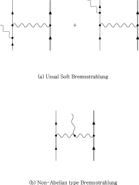
Figure 1: Soft Bremsstrahlung in the NCQED (tree level)

First, consider the diagrams (Fig.1a) for the usual soft Bremsstrahlung. The amplitude $M_{a}$ from the diagram (a) is

$$iM_{a} = e^{\frac{i}{2}(p_{1}\cdot\tilde{p_{1}^{\prime}}+p_{2}\cdot\tilde{p^{\prime}_{2}})}\bar{u}(p_{1}^{\prime})\Biggl{[}M_{0}(p_{1}^{\prime},p-k)\frac{i({\not\!{p_{1}}}-{\not\!{k}}+m)}{(p_{1}-k)^{2}-m^{2}}\gamma^{\rho}\epsilon^{*}_{\rho}(k){e^{\frac{i}{2}g\theta{k}}}$$ (1)

$$+{\gamma^{\rho}}{\epsilon^{*}_{\rho}(k)}{e^{-\frac{i}{2}g\theta{k}}}\frac{{i}(\not\!{p_{1}}+\not\!{k}+m)}{(p_{1}+k)^{2}-m^{2}}M_{0}(p_{1}^{\prime}+k,p)\Biggr{]}\bar{u}(p^{\prime}_{2})\frac{-ig_{\mu\nu}}{q^{2}}(-ie\gamma^{\nu})u(p_{2}).$$

In the above equation, $M_{0}$ is $-ie\gamma^{\mu}$ at the tree level and ${e^{\frac{i}{2}g\theta{k}}}$, ${e^{-\frac{i}{2}g\theta{k}}}$ are reduced from the noncommutative phase factors. Since we are interested in the IR limit, we assume the radiated photon being soft: $|k|\ll|p^{\prime}_{1}-p|$. Then we can approximate

$$M_{0}(p^{\prime},p-k)\approx M_{0}(p^{\prime}_{1}+k,p)\approx M_{0}(p^{\prime},p)$$ (2)

and can ignore $\not\!{k}$ in the numerators of the propagators. The numerators can be further simplified with some Dirac algebra. In the first term we have

$$(\not\!{p}+m)\gamma^{\rho}\epsilon^{*}_{\rho}u(p) = \left[2p^{\rho}\epsilon^{*}_{\rho}+\gamma^{\rho}\epsilon^{*}_{\rho}(-\not\!{p}+m)\right]u(p)$$ (3)

$$= 2p^{\rho}\epsilon^{*}_{\rho}u(p)$$

The denominators of the propagators are also simplified:

$$(p-k)^{2}-m^{2}=-2p\cdot k; (p^{\prime}+k)^{2}-m^{2}=2p^{\prime}\cdot k.$$ (4)

Hence in the soft-photon approximation, the amplitude becomes

$$iM_{a}=\bar{u}(p^{\prime}_{1})[M_{0}(p^{\prime}_{1},p_{1})]u(p_{1})\left[e\cdot\left(\frac{p^{\prime}_{1}\cdot\epsilon^{*}}{p^{\prime}_{1}\cdot k}e^{\frac{i}{2}g\theta{k}}-\frac{p_{1}\cdot\epsilon^{*}}{p_{1}\cdot k}e^{-\frac{i}{2}g\theta{k}}\right)\right]$$ (5)

This is nothing but the amplitude for elastic scattering (without bremsstrahlung)times a factor(in brackets) for the emission of the photon [17].

In the case of Non-abelian type Bremsstrahlung (Fig.1b), the amplitute $M_{b}$ becomes

$$iM_{b} = e^{\frac{i}{2}(p_{1}\cdot\tilde{p_{1}^{\prime}}+p_{2}\cdot\tilde{p^{\prime}_{2}})}\bar{u}(p^{\prime}_{1})(-ie\gamma^{\mu})u(p_{1})\frac{-ig_{\mu\alpha}}{{q^{\prime}}^{2}}\frac{-g_{\beta\nu}}{q^{2}}\epsilon^{*}_{\rho}(k)\biggl{[}B\biggr{]}\bar{u}(p^{\prime}_{2})(-ie\gamma^{\nu})u(p_{2})$$ (6)

where $[B]\;$ is the phase factor for the three photon vertex(Non-Abelian type) given by

$$\biggl{[}B\biggr{]}=-2e\sin\Bigl{(}\frac{k\cdot\tilde{q^{\prime}}}{2}\Bigr{)}\biggl{[}g^{\rho\alpha}(k-q)^{\beta}+g^{\alpha\beta}(q+q^{\prime})^{\rho}+g^{\beta\rho}(-q^{\prime}-k)^{\alpha}\biggr{]}$$ (7)

This is simplified as

$$iM_{b} = e^{\frac{i}{2}(p_{1}\cdot\tilde{p_{1}^{\prime}}+p_{2}\cdot\tilde{p^{\prime}_{2}})}\bar{u}(p^{\prime}_{1})(-ie\gamma^{\mu})u(p_{1})\frac{2e\sin\Bigl{(}\frac{k\cdot\tilde{q^{\prime}}}{2}\Bigr{)}}{(q-k)^{2}q^{2}}\epsilon^{*}_{\rho}$$ (8)

$$\biggl{[}g^{\rho}_{\mu}(k-q)_{\nu}+g_{\mu\nu}(q+q^{\prime})^{\rho}+g^{\rho}_{\nu}(-q^{\prime}-k)_{\mu}\biggr{]}\times\bar{u}(p^{\prime}_{2})(-ie\gamma^{\nu})u(p_{2})$$

There is no IR divergence in this expression. That is, $M_{b}$ is finite for the soft photon : $k\ll|p^{\prime}_{1}-p_{1}|$.

The cross section for the Bremsstrahlung is expressed in terms of the elastic cross section by inserting an additional phase-space integration for the photon variable $k$. Summing over the two photon polarization states, we obtain

$$iM = iM_{a}+iM_{b}$$

$$|M|^{2} = M_{a}^{2}+M_{b}^{2}+M_{a}^{*}M_{b}+M_{a}M_{b}^{*}$$ (9)

In this expression, only $M_{a}^{2}$ contribute to IR divergence. Thus evaluating the cross section only for the usual QED diagram (a), is enough for IR divergence purpose.

$$d\sigma(p\rightarrow p^{\prime}+\gamma) = d\sigma(p\rightarrow p^{\prime})$$

$$\cdot\int\frac{d^{3}k}{(2\pi)^{3}}\frac{1}{2k}\sum_{\lambda=1,2}e^{2}\left|\frac{p^{\prime}\cdot\epsilon^{(\lambda)}}{p^{\prime}\cdot k}{e^{\frac{i}{2}g\theta{k}}}-\frac{p\cdot\epsilon^{(\lambda)}}{p\cdot k}{e^{-\frac{i}{2}g\theta{k}}}\right|^{2}$$

The differential probability of radiating a photon with momentum $k$, given by an election scattered from $p_{1}$ to $p^{\prime}_{1}$, reads

$$d(prob)=\frac{d^{3}k}{(2\pi)^{3}}\sum_{\scriptstyle\lambda}\frac{e^{2}}{2k}\left|\epsilon_{\lambda}\cdot\left(\frac{p^{\prime}_{1}{e^{\frac{i}{2}g\theta{k}}}}{p^{\prime}_{1}\cdot k}-\frac{p{e^{-\frac{i}{2}g\theta{k}}}}{p\cdot k}\right)\right|^{2}$$ (11)

Multiplying by the photon energy $k$ will give the radiated energy.

The equation(11) is an expression not for the expected number of photon radiated, but for the probability of radiating a single photon. The problem becomes worse if we integrate over photon momentum. In order for the soft-photon approximation to be available, the integration upper limit must be restricted. So we will integrate only up to the energy scale where the soft-photon approximation is broken; a reasonable estimate for this energy is $|q|=|p^{\prime}_{1}-p_{1}|$. The integral is therefore

$$\textrm{Total \; probability}\approx\frac{\alpha}{\pi}\int_{0}^{|q|}dk\frac{1}{k}I_{N.C}$$ (12)

where $I_{N.C}$ denote essentially the differential intensity $d$(Energy)/$dk$ for NCQED. We find that the radiative energy at low frequencies($k\rightarrow 0$) is given by

$$I_{N.C} = I_{C}\cdot\cos(q\cdot\tilde{k})$$ (13)

$$\approx 2\log\left(\frac{-q2}{m^{2}}\right)\cdot\cos(q\cdot\tilde{k})$$

where $I_{c}$ represents the differential intensity for the commutative QED. We can regularize the integral in (12) by introducing the very small photon mass $\mu$. This mass would then provide a lower cutoff for the integration over the soft photon momentum,

$$d\sigma(p\rightarrow p^{\prime}+\gamma) = d\sigma(p\rightarrow p^{\prime})\cdot\frac{\alpha}{\pi}\int_{\mu}^{|q|}dk\frac{1}{k}I_{C}\cdot\cos(q\cdot\tilde{k})$$ (14)

$$\approx d\sigma(p\rightarrow p^{\prime})\cdot\frac{\alpha}{\pi}\log\left(\frac{-q^{2}}{\mu^{2}}\right)\log\left(\frac{-q^{2}}{m^{2}}\right)$$

4 Vacuum Polarization in the Noncommutative QED

We consider the 2-point photon self energy diagrams. The contributions are from loops involving fermion, scalars and gauge bosons (Fig.2).

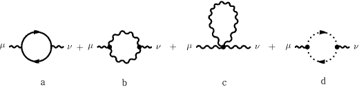
Figure 2: Vacuum polarization in the NCQED

Applying the NC Feynman rules, we find the matrix element $M$ of the photon self energy diagrams.

$$iM = iM^{a}+iM^{b}+iM^{c}+iM^{d}$$ (1)

$$= \bar{u}(p^{\prime}_{1})(-ie\gamma^{\mu})u(p_{1})\frac{-i}{q^{2}}\Bigl{[}i\Pi\Bigr{]}\frac{-i}{q^{2}}\bar{u}(p^{\prime}_{2})(-ie\gamma^{\nu})u(p_{2})$$

where, $i\Pi=i\Pi^{a}_{\mu\nu}+\Pi^{b}_{\mu\nu}+\Pi^{c}_{\mu\nu}+\Pi^{d}_{\mu\nu}$ with

$$i\Pi^{a}_{\mu\nu} = -e^{2}\int\frac{d^{4}k}{(2\pi)^{4}}\frac{\textmd{tr}[\gamma_{\mu}(\not\!{k}+m)\gamma_{\nu}(\not\!{k}-\not\!{q}+m)]}{(k^{2}-m^{2})((k-q)^{2}-m^{2})}$$

$$i\Pi^{b}_{\mu\nu} = -4e^{2}\int\frac{{d^{4}}k}{(2\pi)^{4}}\frac{\sin^{2}\Bigl{(}\frac{k\cdot\tilde{q}}{2}\Bigr{)}{Q_{\mu\nu}}}{(k-q)^{2}{k^{2}}}$$ (2)

$$Q_{\mu\nu}=g_{\mu\nu}(-5q^{2}-2k^{2}+2q\cdot k)+5(k_{\mu}q_{\nu}+k_{\nu}q_{\mu})+2q_{\mu}q_{\nu}-10k_{\mu}k_{\nu}$$

$$i\Pi^{c}_{\mu\nu} = -12e^{2}\int\frac{d^{4}k}{(2\pi)^{4}}\frac{g_{\mu\nu}\sin^{2}\Bigl{(}q\cdot\tilde{k}\Bigr{)}}{k^{2}}$$

$$i\Pi^{d}_{\mu\nu} = -4e^{2}\int\frac{d^{4}k}{(2\pi)^{4}}\frac{(k-q)_{\mu}\sin^{2}\Bigl{(}\frac{q\cdot\tilde{k}}{2}\Bigr{)}}{(k-q)^{2}k^{2}}$$ (3)

All the UV divergences can be subtracted away by the same local counterterms as those in the ordinary QED [10]. Our main concern is the IR divergences of these diagrams. As $q\rightarrow 0$, all diagrams are finite. Hence the structure of the IR divergences is the same as those in the ordinary QED.

5 Vertex structure at the one loop level in NCQED

In this section we perform explicitly the calculation of the vertex function for the photon-electron at the one loop level. Due to the three photon vertices in NCQED, the radiative corrections to the electron-photon vertex come from the two diagrams of Fig 3.

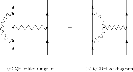
Figure 3: One loop correction to $\psi\bar{\psi}A_{\mu}$ vertex

The invariant matrix element $M$ is given by

$$iM=iM_{1}+iM_{2}.$$ (1)

The $M_{1}$ for the QED-like diagram (Fig3.a) is derived as

$$iM_{1} = e^{\frac{i}{2}(p_{1}\cdot\tilde{p_{1}^{\prime}}+p_{2}\cdot\tilde{p^{\prime}_{2}})}\bar{u}(p^{\prime}_{1})\Bigl{(}-ie\Lambda^{\mu}_{1}(p^{\prime}_{1},p_{1})\Bigr{)}u(p_{1})\times\frac{-ig_{\mu\nu}}{q^{2}}\bar{u}(p^{\prime}_{2})(-ie\gamma^{\nu})u(p_{2})$$ (2)

where

$$\Lambda^{\mu}_{1}(p^{\prime}_{1},p_{1})=\gamma^{\mu}+\Gamma^{\mu}_{1}(p^{\prime}_{1},p_{1})$$

with

$$\Gamma^{\mu}_{1}(p^{\prime},p) = i(-ie)^{2}\int\frac{d^{4}k}{(2\pi)^{4}}e^{-ik\cdot\widetilde{q}}\frac{\gamma^{\rho}}{k^{2}-\mu^{2}+i\epsilon}\frac{\not\!{p^{\prime}}-\not\!{k}+m}{(p^{\prime}-k)^{2}-m^{2}+i\epsilon}\gamma^{\mu}$$ (3)

$$\times \frac{\not\!{p}-\not\!{k}+m}{(p-k)^{2}-m^{2}+i\epsilon}\gamma_{\rho}$$

Here we have added the fictitious photon mass $\mu$ as an IR regulator of the integration.

With the mass shell condition, the numerator in the above expression may be written as

$$4\left\{\gamma^{\mu}\left[(p^{\prime}-k)\cdot(p-k)-\frac{k^{2}}{2}\right]+(p^{\prime}+p-k)^{\mu}\not\!{k}-mk^{\mu}\right\}$$ (4)

We use the following Schwinger parameter representation of the propagators.

$$\frac{i}{p^{2}-m^{2}+i\epsilon}=\int_{0}^{\infty}d\alpha e^{i\alpha(p^{2}-m^{2}+i\epsilon)}$$ (5)

The integral converges at the upper limit owing to the presence of $i\epsilon$. We introduce the following auxiliary integral as the generating function $Z$[18].

$$Z\equiv\int\frac{d^{4}k}{(2\pi)^{4}}e^{ik\cdot(z-\tilde{q})}\frac{1}{(k^{2}-\mu^{2}+i\epsilon)(k^{2}-2p^{\prime}\cdot k+i\epsilon)(k^{2}-2p\cdot k+i\epsilon)}$$

$$=\frac{1}{(4\pi)^{2}}\int_{0}^{\infty}\frac{d\alpha_{1}d\alpha_{2}d\alpha_{3}}{(\alpha_{1}+\alpha_{2}+\alpha_{3})^{2}}exp\left\{-i\left[\alpha_{1}\mu^{2}+\frac{\left(\frac{(z-\tilde{q})}{2}-\alpha_{2}p^{\prime}-\alpha_{3}p\right)^{2}}{\alpha_{1}+\alpha_{2}+\alpha_{3}}\right]\right\}$$

Then the integration with powers of $k$ in the numerator can be obtained by differentiating the above generating function with respect to $z$.

For instance, the integration with $k^{\mu}$ in the numerator is given by

$${\frac{1}{i}\frac{\partial Z}{\partial z_{\mu}}}\mid_{z\rightarrow 0}={-\frac{(\frac{(z-\tilde{q})}{2}-\alpha_{2}p^{\prime}-\alpha_{3}p)^{\mu}}{\alpha_{1}+\alpha_{2}+\alpha_{3}}}Z\mid_{z\rightarrow 0}$$

After symmetrization in $\alpha_{1}$ and $\alpha_{2}$ we obtain the following representation

$$\Gamma^{\mu}_{1}(p^{\prime}_{1},p_{1}) = \frac{\alpha}{i\pi}e^{\frac{i}{2}(p_{1}\cdot\tilde{p_{1}^{\prime}}+p_{2}\cdot\tilde{p^{\prime}_{2}})}\int_{0}^{\infty}\frac{d\alpha_{1}d\alpha_{2}d\alpha_{3}}{(\alpha_{1}+\alpha_{2}+\alpha_{3})^{3}}\Biggl{[}\gamma^{\mu}\biggl{\{}(\alpha_{1}+\alpha_{2}+\alpha_{3})(p^{\prime}_{1}\cdot p_{1})$$ (7)

$$-(\alpha_{2}+\alpha_{3})\frac{(p^{\prime}_{1}+p_{1})^{2}}{2}+p_{1}\cdot\tilde{p^{\prime}_{1}}+\frac{i}{2}+\frac{\left[m^{2}(\alpha_{2}+\alpha_{3})^{2}-\alpha_{2}\alpha_{3}q^{2}\right]}{2(\alpha_{1}+\alpha_{2}+\alpha_{3})}$$

$$-\frac{(\alpha_{2}+\alpha_{3})(p^{\prime}_{1}+p_{1})\cdot\tilde{q}}{4(\alpha_{1}+\alpha_{2}+\alpha_{3})}+\frac{\frac{\tilde{q}^{2}}{4}}{(2\alpha_{1}+\alpha_{2}+\alpha_{3})}\biggr{\}}\Biggr{]}$$

$$\times\exp\frac{i}{\alpha_{1}+\alpha_{2}+\alpha_{3}}\biggl{[}\alpha_{2}\cdot\alpha_{3}q^{2}-(\alpha_{2}+\alpha_{3})^{2}m^{2}$$

$$-\alpha_{1}(\alpha_{1}+\alpha_{2}+\alpha_{3})\mu^{2}+\frac{\alpha_{2}+\alpha_{3}}{2}(p^{\prime}_{1}+p_{1})\cdot\tilde{q}-\frac{\tilde{q}^{2}}{4}\biggr{]}$$

where we have set $p^{\prime}_{1}-p_{1}=q$.

We observe that $q^{2}\leq 0$ if $p_{1}$ and $p^{\prime}_{1}$ lie on the mass shell. Using the identity $1=\int_{0}^{\infty}d\rho\delta(\rho-\alpha_{1}-\alpha_{2}-\alpha_{3})$, changing the variables $\alpha_{i}\rightarrow\rho\alpha_{i}$ and inserting UV regulator $\exp(\frac{i}{\Lambda-\frac{\tilde{q}^{2}}{4}})$, we obtain the following after the Wick rotation $\alpha_{i}\rightarrow-i\alpha_{i}$ :

$${\Gamma^{\mu}_{1}(p_{1}^{{}^{\prime}},p_{1})} = -\frac{\alpha}{\pi}e^{\frac{i}{2}(p_{1}\cdot\tilde{p_{1}^{\prime}}+p_{2}\cdot\tilde{p^{\prime}_{2}})}\int_{0}^{1}{d\alpha_{1}d\alpha_{2}d\alpha_{3}}\delta(1-\Sigma\alpha_{i})\times{e^{-b^{\prime}}}$$ (8)

$$\times\Biggl{[}\gamma^{\mu}\biggl{(}G^{(1)}_{a}\int_{0}^{\infty}{d\rho}e^{-({a\rho}+b/{\rho})}+(G^{(1)}_{b}+G^{(1)}_{c})\int_{0}^{\infty}\frac{d\rho}{\rho}e^{-({a\rho}+b/{\rho})}$$

$$+G^{(1)}_{b^{{}^{\prime}}}\int_{0}^{\infty}\frac{d\rho}{\rho^{2}}e^{-({a\rho}+b/{\rho})}\biggr{)}+\Bigl{\{}H^{\mu,(1)}_{a}\int_{0}^{\infty}{d\rho}e^{-({a\rho}+b/{\rho})}$$

$$+H^{\mu,(1)}_{b}\int_{0}^{\infty}\frac{d\rho}{\rho}e^{-({a\rho}+b/{\rho})}+H^{\mu,(1)}_{b^{{}^{\prime}}}\int_{0}^{\infty}\frac{d\rho}{\rho^{2}}e^{-({a\rho}+b/{\rho})}\Bigr{\}}\Biggr{]}$$

$$-(p^{{}^{\prime}}=p,q=0)$$

where

$$G^{(1)}_{a} = p_{1}\cdot{p_{1}}^{{}^{\prime}}-\frac{(\alpha_{2}+\alpha_{3})(p_{1}^{{}^{\prime}}+p_{1})^{2}}{2}+\frac{1}{2}\left\{m^{2}(\alpha_{2}+\alpha_{3})^{2}-\alpha_{2}\alpha_{3}q^{2}\right\}$$

$$G^{(1)}_{b} = i\left[\frac{1}{2}(p_{1}^{{}^{\prime}}+p_{1})\cdot\widetilde{q}-\frac{1}{4}(\alpha_{2}+\alpha_{3})(p_{1}^{{}^{\prime}}+p_{1})\cdot\widetilde{q}\right],\;\;\;G^{(1)}_{b^{{}^{\prime}}}=-\frac{1}{8}\widetilde{q}^{2}$$

$$G^{(1)}_{c} = -\frac{1}{2},\;\;\;H^{\mu,(1)}_{a}=\frac{m}{2}(p_{1}^{{}^{\prime}}+p_{1})^{\mu}\alpha_{1}(\alpha_{2}+\alpha_{3})$$

$$H^{\mu,(1)}_{b} = i\left[\frac{m}{2}(1+\alpha_{2}+\alpha_{3})\widetilde{q}^{\mu}+\frac{1}{4}(\alpha_{2}+\alpha_{3}-2)(p_{1}^{{}^{\prime}}+p_{1})^{\mu}\widetilde{q}^{\sigma}\gamma_{\sigma}\right]$$

$$H^{\mu,(1)}_{b^{{}^{\prime}}} = \frac{1}{4}\widetilde{q}^{\mu}\widetilde{q}^{\nu}\gamma_{\nu}$$ (9)

and

$$a = -\alpha_{2}\alpha_{3}q^{2}+(\alpha_{2}+\alpha_{3})^{2}m^{2}+\alpha_{1}\mu^{2}$$

$$b = \frac{1}{\Lambda^{2}_{eff}}(={\Lambda^{-2}+\tilde{b}})\;\;(\tilde{b}=-\frac{1}{4}\widetilde{q}^{2})$$

$$b^{\prime} = \frac{i}{2}(\alpha_{2}+\alpha_{3})(p_{1}^{{}^{\prime}}+p_{1})\cdot\widetilde{q}$$ (10)

The Lorentz structure of the terms with $G$ are from the $\gamma^{\mu}$ while those of $H^{\mu}$ not. The constant $a$ and the terms with subscripts $a,c$ are those appearing in the ordinary QED. On the other hands, the constants $b,b^{\prime}$ and the terms with subscripts $b,b^{\prime}$ are the additional terms coming from the noncommutative effects. Hence, if we take the noncommutative parameter $\theta$ going to zero limit, then the terms with subscripts $b,b^{\prime}$ go to zero and the results are those of the ordinary QED.

The integrands with subscripts $b$ and $c$ are proportional to one over $\rho$ while those with $b^{\prime}$ are one over $\rho^{2}$. If we evaluate $\rho$ integral, we get Bessel functions of the following form,

$$\int_{0}^{\infty}d\rho e^{-D} = \int_{0}^{\infty}d\rho e^{-(a\rho+{b\over\rho})}={1\over a}\int_{0}^{\infty}d\rho e^{-(\rho+{ab\over\rho})}$$

$$= {1\over a}\Big{\{}2\sqrt{ab}K[1,2\sqrt{ab}]\Big{\}}$$

$$\int_{0}^{\infty}{d\rho\over\rho}e^{-D} = \int_{0}^{\infty}{d\rho\over\rho}e^{-(\rho+{ab\over\rho})}=\Big{\{}2K[0,\sqrt{ab}]\Big{\}}$$

$$\int_{0}^{\infty}{d\rho\over\rho^{2}}e^{-D} = a\int_{0}^{\infty}{d\rho\over\rho^{2}}e^{-(\rho+{ab\over\rho})}=a\left\{{2\over\sqrt{ab}}K[1,2\sqrt{ab}]\right\}$$

where $K_{0}$, $K_{1}$ are the modified Bessel function.

With the above results of the integral over $\rho$, we get

$$\Gamma^{\mu}_{1}(p^{\prime}_{1},p_{1})=-\frac{\alpha}{\pi}e^{\frac{i}{2}(p_{1}\cdot\tilde{p_{1}^{\prime}}+p_{2}\cdot\tilde{p^{\prime}_{2}})}\int_{0}^{1}d\alpha_{1}d\alpha_{2}d\alpha_{3}\delta(1-\sum\alpha_{i})e^{-i(\alpha_{2}+\alpha_{3})(p^{\prime}_{1}+p_{1})\cdot\tilde{q}}$$

$$\Biggl{(}\gamma^{\mu}\biggl{\{}G^{(1)}_{a}\frac{2\sqrt{ab}K_{1}(a\sqrt{ab})}{a}+(G^{(1)}_{b}+G^{(1)}_{c})2K_{0}(2\sqrt{ab})+G^{(1)}_{b^{\prime}}\frac{aK_{1}(2\sqrt{ab})}{\sqrt{ab}}\biggr{\}}$$

$$+H^{\mu,(1)}_{a}\frac{2\sqrt{ab}K_{1}(a\sqrt{ab})}{a}+H^{\mu,(1)}_{b}2K_{0}(2\sqrt{ab})+H^{\mu,(1)}_{b^{\prime}}\frac{aK_{1}(2\sqrt{ab})}{\sqrt{ab}}\Biggr{)}$$

We now evaluate the matrix element $M_{2}$ for the second QCD-like diagram(Figure3 (b)). It becomes

$$iM_{2}=\bar{u}(p^{\prime}_{1})\Bigl{(}-ie\Lambda^{\mu}_{2}(p^{\prime}_{1},p_{1})\Bigr{)}u(p_{1})\frac{-ig_{\mu\nu}}{q^{2}}\bar{u}(p^{\prime}_{2})(-ie\gamma^{\nu})e^{\frac{i}{2}(p_{2}\cdot\tilde{p^{\prime}_{2}})}u(p_{2})$$ (13)

where $\Lambda^{\mu}_{2}(p^{\prime}_{1},p_{1})=\gamma^{\mu}+\Gamma^{\mu}_{2}(p^{\prime}_{1},p_{1})$, and

$$\Gamma^{\mu}_{2} = \int\frac{d^{4}k}{(2\pi)^{4}}(-ie\gamma^{\nu})e^{\frac{i}{2}(k\cdot\tilde{p^{\prime}_{1}})}\frac{i(\not\!{k}+m)}{k^{2}-m^{2}}(-ie\gamma_{\rho})e^{\frac{i}{2}p_{1}\cdot(\tilde{p_{1}}-\tilde{k})}\frac{-i}{(p^{\prime}_{1}-k)^{2}-\mu^{2}}$$ (14)

$$\times\frac{-i}{(p_{1}-k)^{2}-\mu^{2}}\Biggl{\{}(-2e)\sin{\Bigl{(}\frac{1}{2}(p^{\prime}_{1}-k)\cdot(-\tilde{p}+\tilde{k})\Bigr{)}}$$

$$\times\biggl{[}g^{\nu\rho}(p^{\prime}_{1}+p_{1}-2k)^{\mu}+g^{\rho\mu}(-p_{1}+k+q)^{\nu}+g^{\mu\nu}(-q-p^{\prime}_{1}+k)^{\rho}\biggr{]}\Biggr{\}}$$

$$= i(-ie)^{2}\int\frac{d^{4}k}{(2\pi)^{4}}\frac{e^{\frac{i}{2}(p_{1}\cdot\tilde{p_{1}^{\prime}}+p_{2}\cdot\tilde{p^{\prime}_{2}})}(1-e^{-iq\cdot\tilde{k}}e^{-ip\cdot\tilde{p^{\prime}}})}{[k^{2}-m^{2}][(p_{1}-k)^{2}-\mu^{2}][(p^{\prime}_{1}-k)^{2}-\mu^{2}]}$$

$$\times\biggl{\{}\gamma_{n}u(\not\!{k}+m)\gamma_{\rho}\Bigl{[}g^{\nu\rho}(2k-p^{\prime}_{1}-p_{1})^{\mu}+g^{\rho\mu}(2p_{1}-p^{\prime}_{1}-k)^{\nu}$$

$$+g^{\mu\nu}(2p^{\prime}_{1}-p_{1}-k)^{\rho}\Bigr{]}\biggr{\}}$$

with $p^{\prime}_{1}-p_{1}=q$. Using the mass shell condition and gamma matrix algebra, the numerator can be written as

$$8mk_{\mu}-2\not\!{k}(p^{\prime}+p+2k)_{\mu}+2\gamma_{\mu}(2p^{\prime}.k+2p.k-k^{2}-3m^{2})\$$ (15)

We rewrite the matrix element using the Schwinger parameter representation for the propagators as before.

Here also the introduction of the auxiliary integral as the generating function $Z^{\prime}$ for the various integration is very helpful.

$$Z^{\prime} = \int\frac{d^{4}k}{(2\pi)^{4}}\frac{e^{ik\cdot(z+\tilde{q})}}{(k^{2}-m^{2})((p^{\prime}_{1}-k)^{2}-\mu^{2})((p_{1}-k)^{2}-\mu^{2})}$$

$$= \frac{1}{4\pi^{2}}\int_{0}^{\infty}\frac{d\alpha_{1}d\alpha_{2}d\alpha_{3}}{(\alpha_{1}+\alpha_{2}+\alpha_{3})^{2}}$$

$$\times\exp\Biggl{\{}\frac{-i}{(\alpha_{1}+\alpha_{2}+\alpha_{3})}\biggl{[}\frac{z^{2}}{4}-z\cdot(\alpha_{2}p^{\prime}_{1}+\alpha_{3}p_{1}-\frac{\tilde{q}}{2})$$

$$-(\alpha_{2}+\alpha_{3})p_{1}\cdot\tilde{q}+m^{2}(\alpha_{1}-\alpha_{2}-\alpha_{3})(\alpha_{1}+\alpha_{2}+\alpha_{3})$$

$$+\mu^{2}(\alpha_{2}+\alpha_{3})(\alpha_{1}+\alpha_{2}+\alpha_{3})+m^{2}(\alpha_{2}+\alpha_{3})^{2}-\alpha_{2}\alpha_{3}q^{2}-b\biggr{]}\Biggr{\}}$$

where we have inserted a UV regulator, $b=\frac{1}{\Lambda^{2}_{eff}}(={\Lambda^{-2}+\tilde{b}})\;\;(\tilde{b}=-\frac{1}{4}\widetilde{q}^{2})$.

The integration with various powers of $k$ in the numerator is produced through the derivatives over the $Z^{\prime}$. Inserting the identity $1=\int_{0}^{\infty}d\rho\delta(\rho-\alpha_{1}-\alpha_{2}-\alpha_{3})\;$, rescaling $\alpha_{i}\rightarrow\rho\alpha_{i}\;$, and Wick rotation, we finally obtain

$$\Gamma^{\mu}_{2} = \frac{-\alpha}{\pi}e^{\frac{i}{2}(p_{1}\cdot\tilde{p_{1}^{\prime}}+p_{2}\cdot\tilde{p^{\prime}_{2}})}\int_{0}^{1}d\alpha_{1}d\alpha_{2}d\alpha_{3}\delta(1-\sum\alpha_{i})e^{i(\alpha_{2}+\alpha_{3})p_{1}\cdot\tilde{q}}e^{-ip\cdot\tilde{p^{\prime}}}$$ (17)

$$\times \Biggl{[}\gamma^{\mu}\biggl{(}G^{(2)}_{a}\int_{0}^{\infty}{d\rho}e^{-({a\rho}+b/{\rho})}+(G^{(2)}_{b}+G^{(2)}_{c})\int_{0}^{\infty}\frac{d\rho}{\rho}e^{-({a\rho}+b/{\rho})}$$

$$+G^{(2)}_{b^{{}^{\prime}}}\int_{0}^{\infty}\frac{d\rho}{\rho^{2}}e^{-({a\rho}+b/{\rho})}\biggr{)}+\Bigl{\{}H^{\mu,(2)}_{a}\int_{0}^{\infty}{d\rho}e^{-({a\rho}+b/{\rho})}$$

$$+H^{\mu,(2)}_{b}\int_{0}^{\infty}\frac{d\rho}{\rho}e^{-({a\rho}+b/{\rho})}+H^{\mu,(2)}_{b^{{}^{\prime}}}\int_{0}^{\infty}\frac{d\rho}{\rho^{2}}e^{-({a\rho}+b/{\rho})}\Bigr{\}}\Biggr{]}$$

$$+ \frac{-\alpha}{\pi}e^{\frac{i}{2}(p_{1}\cdot\tilde{p_{1}^{\prime}}+p_{2}\cdot\tilde{p^{\prime}_{2}})}\int_{0}^{1}d\alpha_{1}d\alpha_{2}d\alpha_{3}\delta(1-\sum\alpha_{i})$$

$$\times\Biggl{[}\gamma^{\mu}\biggl{(}G^{(2)}_{a}\int_{0}^{\infty}{d\rho}e^{-({a\rho}+b^{\prime}/{\rho})}+G^{(2)}_{c}\int_{0}^{\infty}\frac{d\rho}{\rho}e^{-({a\rho}+b^{\prime}/{\rho})}\biggr{)}$$

$$+\Bigl{\{}H^{\mu,(2)}_{a}\int_{0}^{\infty}{d\rho}e^{-({a\rho}+b^{\prime}/{\rho})}\Bigr{\}}\Biggr{]}-(p^{{}^{\prime}}=p,q=0)$$

where,

$$G^{(2)}_{a} = \frac{1}{2}\Bigl{[}(\alpha_{2}+\alpha_{3})(p^{\prime}_{1}+p_{1})^{2}-3m^{2}-m2(\alpha_{2}+\alpha_{3})^{2}+\alpha_{2}\alpha_{3}q^{2}\Bigr{]}$$

$$G^{(2)}_{b} = \frac{-i}{2}p_{1}\cdot\tilde{q}(2-\alpha_{2}-\alpha_{3}),\;\;\;\;G^{(2)}_{b^{\prime}}=\frac{\tilde{q}^{2}}{8},\;\;\;\;G^{(2)}_{c}=\frac{3}{2}$$

$$H^{\mu,(2)}_{a} = \frac{m}{2}(p^{\prime}_{1}+p_{1})^{\mu}\alpha_{1}(\alpha_{2}+\alpha_{3})$$

$$H^{\mu,(2)}_{b} = \frac{-i}{2}(2-\alpha_{2}-\alpha_{3})\tilde{q}^{\mu}+\frac{i}{4}(1+\alpha_{2}+\alpha_{3})(p^{\prime}_{1}+p_{1})^{\mu}\gamma\cdot\tilde{q}$$

$$H^{\mu,(2)}_{b^{\prime}} = \frac{\gamma\cdot\tilde{q}}{4}\tilde{q}^{\mu}$$

with

$$a = m^{2}(\alpha_{1}-\alpha_{2}-\alpha_{3})+\mu^{2}(\alpha_{2}+\alpha_{3})+m^{2}(\alpha_{2}+\alpha_{3})^{2}-\alpha_{2}\alpha_{3}q^{2}$$

$$b = {\Lambda^{2}_{eff}(=\Lambda^{-2}+\tilde{b})}\;\;(\tilde{b}=-\frac{1}{4}\widetilde{q}^{2})$$ (19)

Here also the constant $b$ and terms $G$ or $H$ with the subscripts $b,b^{\prime}$ are the additional quantities coming from the noncommutativity. In the limit of ordinary QED, those values with indices $b$ and $b^{\prime}$ become zero and we get the same result as that in the ordinary QED.

Integration over $\rho$ leads to

$$\Gamma^{\mu}_{2} = \frac{-\alpha}{\pi}e^{\frac{i}{2}(p_{1}\cdot\tilde{p_{1}^{\prime}}+p_{2}\cdot\tilde{p^{\prime}_{2}})}\int_{0}^{1}d\alpha_{1}d\alpha_{2}d\alpha_{3}\delta(1-\sum\alpha_{i})e^{i(\alpha_{2}+\alpha_{3})p_{1}\cdot\tilde{q}}e^{-ip\cdot\tilde{p^{\prime}}}$$ (20)

$$\times\Biggl{[}\gamma^{\mu}\biggl{\{}G^{(2)}_{a}\frac{2\sqrt{ab}K_{1}(a\sqrt{ab})}{a}+(G^{(2)}_{b}+G^{(2)}_{c})2K_{0}(2\sqrt{ab})+G^{(2)}_{b^{\prime}}\frac{aK_{1}(2\sqrt{ab})}{\sqrt{ab}}\biggr{\}}$$

$$\quad\quad\quad+H^{\mu,(2)}_{a}\frac{2\sqrt{ab}K_{1}(a\sqrt{ab})}{a}+H^{\mu,(2)}_{b}2K_{0}(2\sqrt{ab})+H^{\mu,(2)}_{b^{\prime}}\frac{aK_{1}(2\sqrt{ab})}{\sqrt{ab}}\Biggr{]}$$

$$+ \frac{-\alpha}{\pi}e^{\frac{i}{2}(p_{1}\cdot\tilde{p_{1}^{\prime}}+p_{2}\cdot\tilde{p^{\prime}_{2}})}\int_{0}^{1}d\alpha_{1}d\alpha_{2}d\alpha_{3}\delta(1-\sum\alpha_{i})$$

$$\times\Biggl{[}\gamma^{\mu}\biggl{\{}G^{(2)}_{a}\frac{2\sqrt{ab^{\prime}}K_{1}(a\sqrt{ab^{\prime}})}{a}+G^{(2)}_{c}2K_{0}(2\sqrt{ab^{\prime}})\biggr{\}}+H^{\mu,(2)}_{a}\frac{2\sqrt{ab^{\prime}}K_{1}(a\sqrt{ab^{\prime}})}{a}\Biggr{]}$$

We want analyze the divergences in NCQED and compare with those in the ordinary QED, where the logarithmic UV divergences are renormalized and the problem of IR divergences , after regularized by the soft photon mass $\mu$, are cancelled between the bremstrahlung and the radiative loop corrections.

In section 6, we will analyze in detail the IR divergence of NCQED.

The vertex functions contain $K_{0}$ and $K_{1}$, and both of the functions contain either UV regulator $\frac{1}{\Lambda_{eff}^{2}}$ or $\frac{1}{\Lambda^{2}}$ in their arguments. As the high energy limit $\Lambda^{2}\to\infty$, or $b\rightarrow 0$, we find that all terms containing $K_{1}$ are finite, but a logarithmic divergence appears in $K_{0}$. Since the noncommutative QED was shown to be renormalizable up to the one loop level by adding the relevant counter terms, we can safely drop the singular parts in $K_{0}$, keeping only the finite parts.

$$\Gamma^{\mu}_{(R)} = \Gamma^{\mu}_{1(R)}+\Gamma^{\mu}_{2(R)}$$ (21)

$$= \frac{-\alpha e^{\frac{i}{2}(p_{1}\cdot\tilde{p_{1}^{\prime}}+p_{2}\cdot\tilde{p^{\prime}_{2}})}}{\pi}\int_{0}^{1}d\alpha_{1}d\alpha_{2}d\alpha_{3}\delta(1-\sum\alpha_{i})$$

$$\Biggl{[}\frac{(\gamma^{\mu}G^{(1)}_{a}+H^{\mu,(1)}_{a})e^{-i(\alpha_{2}+\alpha_{3})p_{1}\cdot\tilde{q}}}{a}+\frac{(\gamma^{\mu}G^{(2)}_{a}+H^{\mu,(2)}_{a})(1-e^{i(\alpha_{2}+\alpha_{3})p_{1}\cdot\tilde{q}})e^{-ip_{1}\cdot p^{\prime}_{1}}}{a^{\prime}}$$

$$\quad-2\gamma_{E}\biggl{\{}(\gamma^{\mu}G^{(1)}_{b}+\gamma^{\mu}G^{(1)}_{c}+H^{\mu,(1)}_{b})e^{-i(\alpha_{2}+\alpha_{3})p_{1}\cdot\tilde{q}}+\gamma^{\mu}G^{(2)}_{c}$$

$$\quad\quad\quad+(\gamma^{\mu}G^{(2)}_{b}+\gamma^{\mu}G^{(2)}_{c}+H^{\mu,(2)}_{b})e^{-i(\alpha_{2}+\alpha_{3})p_{1}\cdot\tilde{q}}\biggr{\}}$$

$$\quad\Lambda^{2}_{eff}\biggl{\{}\Bigl{(}G^{(1)}_{b^{\prime}}+H^{\mu,(1)}_{b^{\prime}}\Bigr{)}e^{-i(\alpha_{2}+\alpha_{3})p_{1}\cdot\tilde{q}}+\Bigl{(}G^{(2)}_{b^{\prime}}+H^{\mu,(2)}_{b^{\prime}}\Bigr{)}e^{-i(\alpha_{2}+\alpha_{3})p_{1}\cdot\tilde{q}}e^{p_{1}\cdot p^{\prime}_{1}}\biggr{\}}\Biggr{]}$$

The last expressions contain two types of terms, both proportional to $\tilde{q}^{2}$. Since ${\Lambda^{2}}{\tilde{q}^{2}}\ll 1$, in the IR limit, this term is totally irrelevant. One should note that the limits taking ${\Lambda^{2}}\to\infty$ and $q\to 0$, is very important in our arguments. The fully renormalized vertex function is then,

$$\Gamma^{\mu}_{(R)} = \Gamma^{\mu}_{1(R)}+\Gamma^{\mu}_{2(R)}$$ (22)

$$= \frac{-\alpha e^{\frac{i}{2}(p_{1}\cdot\tilde{p_{1}^{\prime}}+p_{2}\cdot\tilde{p^{\prime}_{2}})}}{\pi}\int_{0}^{1}d\alpha_{1}d\alpha_{2}d\alpha_{3}\delta(1-\sum\alpha_{i})$$

$$\Biggl{[}\frac{(\gamma^{\mu}G^{(1)}_{a}+H^{\mu,(1)}_{a})e^{-i(\alpha_{2}+\alpha_{3})p_{1}\cdot\tilde{q}}}{a}+\frac{(\gamma^{\mu}G^{(2)}_{a}+H^{\mu,(2)}_{a})(1-e^{i(\alpha_{2}+\alpha_{3})p_{1}\cdot\tilde{q}})e^{-ip_{1}\cdot p^{\prime}_{1}}}{a^{\prime}}$$

$$\quad-2\gamma_{E}\biggl{\{}(\gamma^{\mu}G^{(1)}_{b}+\gamma^{\mu}G^{(1)}_{c}+H^{\mu,(1)}_{b})e^{-i(\alpha_{2}+\alpha_{3})p_{1}\cdot\tilde{q}}+\gamma^{\mu}G^{(2)}_{c}$$

$$\quad\quad\quad+(\gamma^{\mu}G^{(2)}_{b}+\gamma^{\mu}G^{(2)}_{c}+H^{\mu,(2)}_{b})e^{-i(\alpha_{2}+\alpha_{3})p_{1}\cdot\tilde{q}}\biggr{\}}\Biggl{]}$$

This result is the same as that of I.F.Riad and M.M.Sheikh-Jabbari. [13].

The recent paper [14, 15] shows the 1.6 deviation of the theoretical muon anomalous magnetic moment in the Standard Model (SM) from the experimental data, $a^{\rm exp}_{\mu}-a^{\rm SM}_{\mu}=426(165)\times 10^{-11}$. This result has been treated as an indication of new physics and caused extensive interest in many articles. We study the noncommutative QED up to 1-loop level and correction on muon anomalous magnetic moment due to noncommutativity. The noncommutative QED contribution to $a_{\mu}$ follows.

$$a^{exp}_{\mu}-\tilde{a}{{}^{NC}_{\mu}}=a^{exp}_{\mu}-(a^{QED}_{\mu}+\delta\tilde{a}{{}^{NC}_{\mu}})$$ (23)

The $\tilde{a}{{}^{NC}_{\mu}}$ is obtained by the noncommutative QED ($\tilde{a}{{}^{NC}_{\mu}}=a^{QED}_{\mu}+\delta\tilde{a}{{}^{NC}_{\mu}}$).

From now on, we will study the noncommutative effect to the anomalous magnetic moment. Up to the one loop approximation, $\Gamma^{\mu}_{(R)}$ can be expanded as functions of $q^{2},p_{1}.\tilde{q}~{}~{}\textrm{and}~{}~{}\gamma.\tilde{q}$ with some coefficients

$$\Gamma^{\mu}_{(R)}=A^{\prime}\gamma^{\mu}+B^{\prime}(p^{\prime}+p)^{\mu}+C\tilde{q}^{\mu}+D\gamma^{\mu}p.\tilde{q}+E(p^{\prime}+p)^{\mu}\gamma.\tilde{q}.$$ (24)

The coefficients (from $A^{\prime}$ to $E$) are functions of $G^{i}_{(a,b,c)}$ and $H^{i}_{(a,b,c)}$ in equation (22). In the NCQED, the coefficients, $C$ and $D$ can give a contribution to the magnetic moment. In the low momentum limit[13], the contribution of $D\gamma^{\mu}p.\tilde{q}$ can be ignored and only $C$ gives a main contribution to the magnetic moment. From the effective interaction potential with the external magnetic field $V(x)=-<\mu>\cdot B(x)$, the magnetic moment is given by

$$<\mu>=\frac{c}{i}\theta,$$ (25)

which is exactly the same result of Ref. [13].

The vertex function compatible with the Ward identity can be rewritten as

$$\Gamma^{\mu}=A\gamma^{\mu}+B(p^{\prime}_{1}+p_{1})^{\mu}+C\tilde{q}^{\mu},$$ (26)

where $A$ is a function of $A^{\prime}$ and $D$ and $B$ a function of $B^{\prime}$ and $E$, respectively. In the high momentum limit, the contribution linearly proportional to $\theta$ and the momentum $p$ as well as the previous one evaluated in the low momentum limit, must be considered. To evaluate the contribution of the former, we use the form factors $F_{1}(q^{2})~{}~{}\textrm{and}~{}~{}F_{2}(q^{2})$, which is expressed as functions of $A~{}~{}\textrm{and}~{}~{}B$ using the Gordon identity and then the invariant matrix element $M$ is given by

$$iM=-ie\xi^{\dagger}\left(-\frac{-\sigma_{k}}{2m}[F_{1}(0)+F_{2}(0)]\right)\xi\tilde{B}^{k}(q).$$ (27)

Note that $M$ can be considered as the Born approximation to the scattering of the electron with the potential

$$iM = -2mi\hat{V}({\bf q})=-2mi\Big{(}-\mu^{k}\hat{B}^{k}\Big{)}$$ (28)

$$= -2miie\theta G_{1}\hat{B}^{3}$$

$$\mu^{1}=\mu^{2}=0 \mu^{3}(\theta)=-ieG_{1}\theta,$$ , (29)

where only $\mu^{3}$ component appears due to our choice of noncommutativity between $x^{1}$ and $x^{2}$. From (22), the noncommutative correction to the magnetic moment is obtained from the following

$$\widetilde{F_{2}} = -{\frac{\alpha}{\pi}}{e^{\frac{i}{2}(p_{1}\cdot\tilde{p_{1}^{\prime}}+p_{2}\cdot\tilde{p^{\prime}_{2}})}}{\int_{0}^{1}d\alpha_{1}d\alpha_{2}d\alpha_{3}\delta(1-\sum\alpha_{i})}\;[A+B]$$ (30)

$$A =\frac{m^{2}\alpha_{1}(\alpha_{2}+\alpha_{3})e^{i(\alpha_{2}+\alpha_{3})p\cdot\tilde{q}}}{\alpha_{1}\mu^{2}+(\alpha_{2}+\alpha_{3})^{2}m^{2}-\alpha_{2}\alpha_{3}q^{2}}$$

$$B =\frac{m^{2}\alpha_{1}(\alpha_{2}+\alpha_{3})(1-e^{(\alpha_{2}+\alpha_{3})p\cdot\tilde{q}})e^{-i(p_{1}\cdot\tilde{p_{1}}+p_{2}\cdot\tilde{p_{2}})}}{m^{2}(\alpha_{1}-\alpha_{2}-\alpha_{3})+\mu^{2}(\alpha_{2}+\alpha_{3})+m^{2}(\alpha_{2}+\alpha_{3})+m^{2}(\_2+\alpha_{3})^{2}-\alpha_{2}\alpha_{3}q^{2}},$$

where $A$ is the contribution of the first diagram and $B$ denotes the effects of the second diagram (Figure 3.). Using the following approximation $e^{iab}\approx 1+iab+(\frac{iab}{2})^{2}+\cdots$, the above equation can be rewritten as

$$\widetilde{F_{2}} = -{\frac{\alpha}{\pi}}{e^{\frac{i}{2}(p_{1}\cdot\tilde{p_{1}^{\prime}}+p_{2}\cdot\tilde{p^{\prime}_{2}})}}{\int_{0}^{1}d\alpha_{1}d\alpha_{2}d\alpha_{3}\delta(1-\sum\alpha_{i})}\;[\widetilde{A}+\widetilde{B}]$$ (31)

$$\widetilde{A} =\frac{m^{2}\alpha_{1}(\alpha_{2}+\alpha_{3})[1-\frac{1}{2}(\alpha_{2}+\alpha_{3})^{2}(p\theta q)^{2}]}{\alpha_{1}\mu^{2}+(\alpha_{2}+\alpha_{3})^{2}m^{2}-\alpha_{2}\alpha_{3}q^{2}}$$

$$\widetilde{B} =-\frac{m^{2}\alpha_{1}(\alpha_{2}+\alpha_{3})\left[(\alpha_{2}+\alpha_{3})(p\theta q)+\frac{1}{2}(\alpha_{2}+\alpha_{3})^{2}(p\theta q)^{2}\right]}{m^{2}(\alpha_{1}-\alpha_{2}-\alpha_{3})+\mu^{2}(\alpha_{2}+\alpha_{3})+m^{2}(\alpha_{2}+\alpha_{3})+m^{2}(\alpha_{2}+\alpha_{3})^{2}-\alpha_{2}\alpha_{3}q^{2}}$$

where we ignore the imaginary parts and higher order terms of $\theta$. Before starting the calculation for $\widetilde{F_{2}}$, the $\theta$ independent magnetic moment which comes from the ordinary QED, can be derived from the $\theta$ independent terms in $\widetilde{A}$ and here we omit the evaluation of the magnetic moment of QED. Since we want to consider the correction of the magnetic moment caused by the noncommutativity and related to the first order of $\theta$, from now on we will pay attention to the term which linearly depends on $\theta$ in $\widetilde{B}$. Since the photon mass, $\mu$ was introduced as a IR cutoff for removing the divergence due to the zero momentum of the photon, we will set $\mu$ very small ($\mu\rightarrow 0$). In the case of the soft photon ($q\rightarrow 0$), a leading noncommutative correction term $\widetilde{F_{2}}(\theta\neq 0)$ reads

$$\widetilde{F_{2}}(\theta\neq 0) = \frac{\alpha(p\theta q)}{\pi}{\int_{0}}^{1}d\alpha_{2}d\alpha_{3}\;\frac{\{1-(\alpha_{2}+\alpha_{3})\}(\alpha_{2}+\alpha_{3})^{2}}{(\alpha_{2}+\alpha_{3})^{2}-(\alpha_{2}+\alpha_{3})+1}$$ (32)

$$= -0.074\times\frac{\alpha(p\theta q)}{\pi}.$$

This noncommutative correction term linearly depends on the photon momentum $q$ and the noncommutative parameter $\theta$ and is important in the higher momentum limit. Therefore the total magnetic moment is summarized as the following

$$\langle\vec{\mu}\rangle_{tot}=\langle\vec{\mu}\rangle_{0}+\vec{\mu}_{corr}(\theta),$$ (33)

where $\langle\vec{\mu}\rangle_{0}$ is the magnetic moment coming from the ordinary QED. The noncommutative correction term $\vec{\mu}_{corr}(\theta)$ is given by

$$\vec{\mu}_{corr}(\theta)=\frac{\alpha\gamma_{Euller}}{6\pi}em\vec{\theta}-0.074\frac{e\alpha(p\theta q)}{\pi m}\xi^{\dagger}{\vec{\sigma}\over 2}\xi.$$ (34)

Here the first term is the leading noncommutative correction, which is consistent with the result in Ref. [13]. The second one is derived in the high momentum limit and so its effect in the low momentum limit can be ignored. In Ref. [16], it was argued that these kinds of noncommutative corrections can make the SM prediction of the anomalous magnetic moment close to the experimental data.

6 Interpretation of IR divergences for the one loop level

In the previou section we evaluated the NCQED process up to one loop diagrams. We confirmed that the vacuum polarization diagrams have no IR divergences while the soft bremsstrahlung diagrams have the similar IR properties as in ordinary QED. In equation (24), Gordon decomposition is modified with extra piece in NCQED. By renormalization condition for one-loop correction in NCQED, the modified form factor $F^{{}^{\prime}(ren)}_{1}$ is ,

$$F^{{}^{\prime}(ren)}_{1}(q^{2})=F^{\prime}_{1}(q^{2})-F^{\prime}_{1}(0)$$ (1)

Now let us confront with the IR divergence in our result (22) for $F^{{}^{\prime}(ren)}_{1}(q^{2})$ in the vertex function. The calculation for $F^{{}^{\prime}(ren)}_{1}(q^{2})$ is much more difficult. However, it will be important in resolving the question of the IR divergence, which we found in the discussion of bremsstrahlung. We will find that the IR divergence coming from the bremsstrahlung diagram and $F^{{}^{\prime}(ren)}_{1}(q^{2})$ cancel exactly even for finite noncommutativity $\theta$. Although the calculation of $F^{{}^{\prime}(ren)}_{1}(q^{2})$ is difficult, one can extract useful information from by taking the limit as $\mu$ becomes small. Then $F^{{}^{\prime}(ren)}_{1}(q^{2})$ integration in (24) splits up into some pieces:

$$F^{{}^{\prime}(ren)}_{1}(q^{2})=\sum^{N}_{i=1}P_{i}+\cdots$$ (2)

where the ellipsis represents constant terms.

In the IR limit, $\mu\rightarrow 0$, the dominant part, is

$$F^{{}^{\prime}(ren)}_{1}(q^{2}) = \frac{-\alpha e^{\frac{i}{2}(p_{1}\cdot\tilde{p_{1}^{\prime}}+p_{2}\cdot\tilde{p^{\prime}_{2}})}}{\pi}\int_{0}^{1}d\alpha_{1}d\alpha_{2}d\alpha_{3}\delta(1-\sum\alpha_{i})$$ (3)

$$\quad\times\frac{(p_{1}\cdot{p_{1}}^{{}^{\prime}})e^{-i(\alpha_{2}+\alpha_{3})p_{1}\cdot\tilde{q}}}{-\alpha_{2}\alpha_{3}q^{2}+(\alpha_{2}+\alpha_{3})^{2}m^{2}+\alpha_{1}\mu^{2}}$$

The result for the ordinary QED is in the same form except the tildes.

Under the limit $e^{i{x\over 2}p_{1}\tilde{q}}\approx 1+i{x\over 2}p_{1}\tilde{q}+\cdots$ we find $F^{\prime}_{1}$

$$F^{{}^{\prime}(ren)}_{1}(q^{2}) = {-\alpha\over\pi}\int_{0}^{1}d\alpha_{3}\int_{0}^{1}dx{x(m^{2}-{q^{2}\over 2})\over{x^{2}\{(m^{2}-(\alpha_{3}-\alpha_{3}^{2})q^{2}\}+\mu^{2}(1-x)}}$$ (4)

$$= {-\alpha\over 2\pi}\left(m^{2}-{q^{2}\over 2}\right)\bigg{[}\int_{0}^{1}d\alpha_{3}{\log\{m^{2}-(\alpha_{3}-\alpha_{3}^{2})q^{2}\}\over{m^{2}-(\alpha_{3}-\alpha_{3}^{2})q^{2}}}$$

$$-\log{\mu^{2}\over m^{2}}\int_{0}^{1}d\alpha_{3}{1\over{m^{2}-(\alpha_{3}-\alpha_{3}^{2})q^{2}}}\bigg{]}$$

$$\approx \frac{\alpha}{\pi}\Biggl{[}\biggl{(}\log\frac{\mu}{m}+1\biggr{)}(\theta\coth\theta-1)-2\coth\int_{0}^{\theta\over 2}d\phi\phi\tanh\phi-\frac{\theta}{4}\tanh\frac{\theta}{2}\Biggr{]}$$

where,

$$p^{\prime}_{1}\cdot p_{1}=m^{2}\cosh\theta;\;q^{2}=-4m^{2}\sinh^{2}(\theta/2)$$ (5)

For $|q^{2}|\gg m^{2}$ we find,

$$\gamma^{\mu}+\Gamma^{\mu}\sim\gamma^{\mu}\biggl{\{}1-\frac{\alpha}{\pi}\log\frac{m}{\mu}\Bigl{[}\log\Bigl{(}\frac{-q^{2}}{m^{2}}\Bigr{)}-1+O(\frac{m^{2}}{q^{2}})\Bigr{]}\biggr{\}}$$ (6)

Plugging all this into cross-section formula, we now find our final result,

$$\frac{d\sigma}{d\Omega}(p\rightarrow p^{\prime})=\frac{d\sigma}{d\Omega}_{0}\Biggl{[}1-\frac{\alpha}{\pi}\log\Bigl{(}\frac{-q^{2}}{m^{2}}\Bigr{)}\log\Bigl{(}\frac{-q^{2}}{\mu^{2}}\Bigr{)}+O(\alpha^{2})\Biggr{]}$$ (7)

We recall that bremsstrahlung amplitude in Eq.(14) in limit $|q^{2}|\gg m^{2}$

$$d\sigma(p\rightarrow p^{\prime}+\gamma) \approx d\sigma(p\rightarrow p^{\prime})\cdot\frac{\alpha}{\pi}\log\left(\frac{-q^{2}}{\mu^{2}}\right)\log\left(\frac{-q^{2}}{m^{2}}\right)$$ (8)

In fact, neither the elastic cross section nor the soft bremsstrahlung cross section can be measured individually; only their sum is physically observable. In any experiment, a photon vdetector can detect photons only down to some minimum limiting energy $E_{l}$. The probability that a scattering event occurs and this detector does not see a photon is the sum.

$$\frac{d\sigma}{d\Omega}(p\rightarrow p^{\prime})+\frac{d\sigma}{d\Omega}(p\rightarrow p^{\prime}+\gamma(k<E_{l}))\equiv\left(\frac{d\sigma}{d\Omega}\right)_{\scriptstyle{measured}}$$ (9)

Clearly, we find a finite,convergent result independent of $\mu^{2}$, as claimed.

$$\frac{d\sigma}{d\Omega}(p\rightarrow p^{\prime})_{\scriptstyle{measured}}\approx\frac{d\sigma}{d\Omega}_{0}\Biggl{[}1-\frac{\alpha}{\pi}\log\Bigl{(}\frac{-q^{2}}{m^{2}}\Bigr{)}\log\Bigl{(}\frac{-q^{2}}{E^{2}_{l}}\Bigr{)}+O(\alpha^{2})\Biggr{]}$$ (10)

7 Discussion

In this work we have analysed some aspects of NCQED up to one loop level. The diagrams for NCQED contain non-abelian type diagrams. There are additional non-abelian type diagrams in the photon vacuum polarization, and electron-photon interaction vertex. All the UV divergences can be subtracted away by the same local counterterms as in the ordinary QED. The main analysis of this work is for the IR divergence.

We analysed the soft bremsstrahlung diagrams, which is correlated to the IR divergence of the vertex function.

First of all, the IR divergence of the soft bremsstrahlung diagrams in the NCQED at finite noncommutativity are the same result as that in the ordinary QED. The IR divergences of the bremsstrahlung is shown to be cancelled out by divergence of vertex function in NCQED also. In vacuum polarization diagrams, there is no IR divergence as in QED.

In section 5, we performed explicit calculation of the vertex function for the photon-electron at one loop level. In that case, it contribute to the anomalous magnetic moment and there is a generic feature of noncommutative field theory, UV/IR mixing.

In vertex function, we argued that the photon itself, similar to the moving noncommutative electron, shows some electric dipole effect and magnetic dipole moment of electron has now two parts; one is spin dependent part which will not receive any further corrections due to the noncommutativity and the other is spin independent, being proportional to $\theta$. In this paper, we have calculated all noncommutative corrections proportional to $\theta$.

We have found cancellation of the IR divergence of the electron vertex function by the soft bremsstrahlung in the ordinary QED. In the NCQED case, Feynman diagrams show additional non-Abelian typed diagram from the vertex function and vacuum polarization. Nevertheless IR divergences of all diagrams the same results as that of the ordinary QED.

Acknowledgments This work was supported by the Korea Research Foundation, Grant No. KRF-2001-DP0083. BHL is also supported by the Sogang University Research Grant in 2001.

References

• [1] A. Connes, M. R. Douglas, and A. Schwarz, Noncommutative geometry and matrix theory on tori, J.Β High Β Energy Β Phys. 9802 (1998) 003.
• [2] M. R. Douglas and C. Hull, D-branes and the Noncommutative Torus, J.Β High Β Energy Β Phys. 02 (1998) 008, hep-th/9711165
• [3] T. Banks, W. Fischler, S. H. Shenker, and L. Susskind, Phys.Β Rev. D55 (1997) 5112.
• [4] N. Ishibashi, H. Kawai, Y. Kitazawa, and A. Tsuchiya, Nucl.Β Phys. B498 (1997) 467.
• [5] N. Seiberg and E. Witten , String Theory and Noncommutative Geometry J.Β High Β Energy Β Phys. 09 (1999) 032, hep-th/9908142
• [6] S. Minwalla, M. Van Raamsdonk, N. Seiberg, Noncommutative Perturbative Dynamics, hep-th/9912072.
• [7] C.P. Martin, D. Sanchez-Ruiz, Phys. Rev. Lett. 83 (1999) 476;
• [8] I. Ya. Aref’eva, D.M. Belov, A.S. Koshelev, Two-Loop Diagrams in Noncommutative $\varphi^{4}_{4}$ Theory, Phys. Lett. B476 (2000) 431. hep-th/9912075.
• [9] A. Matusis, L. Susskind, N. Toumbas, The IR/UV Connection in the Noncommutative Gauge Theories, hep-th/0002075. D.Β Bigatti and L.Β Susskind, Magnetic fields, branes and noncommutative geometry, hep-th/9908056.
• [10] M.Hayakawa, Perturbative analysis on infrared and ultraviolet aspects of noncommutative QED on $R^{4}$,Phys.Β Lett. B478 (2000) 394, hep-th/9912167 bibitem12
• [11] F. Ardalan, N. Sadooghi, Axial Anomaly in Non-Commutative QED on $R^{4}$, hep-th/0002143.
• [12] L. Alvarez-Gaume, S. R. Wadia, Gauge Theory on a Quantum Phase Space, hep-th/0006219.
• [13] I.F.Riad and M.M.Sheikh-Jabbari, Noncommutative QED and Anomalous Dipole Moments, J.Β High Β Energy Β Phys. 08 (2000) 045 , hep-th/0008132.
• [14] H.Β N.Β Brown [Muon g-2 Collaboration], hep-ex/0102017.
• [15] M. Hayakawa and T. Kinoshita, Comment on the sign of the pseudoscalar ploe contribution to the muon g-2, hep-th/0112102.
• [16] Xiao-Jun Wang, Mu-Lin Yan, Noncommutative QED and Muon Anomalous Magnetic Moment, hep-th/0109095.
• [17] M.E.Peskin and D.v.Schroeder An Introduction to Quantum Field Theory, Addison-Wesley Publishing Company, 1995.
• [18] C.Itzykson and J-B. Zuber, Quantum Field Theory, McGraw-Hill, 1985.