PP-wave string interactions
from perturbative Yang-Mills theory

Abstract:

Recently, Berenstein et al. have proposed a duality between a sector of $\N=4$ super-Yang-Mills theory with large R-charge $J$, and string theory in a pp-wave background. In the limit considered, the effective ’t Hooft coupling has been argued to be $\lambda^{\prime}=g_{\rm YM}^{2}N/J^{2}=1/(\mu p^{+}\apm)^{2}$. We study Yang-Mills theory at small $\lambda^{\prime}$ (large $\mu$) with a view to reproducing string interactions. We demonstrate that the effective genus counting parameter of the Yang-Mills theory is $g^{2}_{2}=J^{4}/N^{2}=(4\pi g_{\rm s})^{2}(\mu p^{+}\apm)^{4}$, the effective two-dimensional Newton constant for strings propagating on the pp-wave background. We identify $g_{2}\sqrt{\lambda^{\prime}}$ as the effective coupling between a wide class of excited string states on the pp-wave background. We compute the anomalous dimensions of BMN operators at first order in $g_{2}^{2}$ and $\lambda^{\prime}$ and interpret our result as the genus one mass renormalization of the corresponding string state. We postulate a relation between the three-string vertex function and the gauge theory three-point function and compare our proposal to string field theory. We utilize this proposal, together with quantum mechanical perturbation theory, to recompute the genus one energy shift of string states, and find precise agreement with our gauge theory computation.

1 Introduction

Many years ago ’t Hooft [1] demonstrated the existence of a nontrivial large $N$ limit of $SU(N)$ gauge theories

$$N\to\infty,~{}~{}~{}g^{2}_{\rm YM}\to 0,~{}~{}~{}\lambda=g_{\text{YM}}^{2}N~{}~{}{\rm fixed}.$$ (1.1)

In the ’t Hooft limit (1.1), Yang-Mills interactions are controlled by the ’t Hooft coupling $\lambda=g_{\text{YM}}^{2}N$. Away from the strict $N\to\infty$ limit, Yang-Mills perturbation theory may be organized as a double expansion. Feynman graphs are summed over their genus (controlled by the genus counting parameter $1/N^{2}$) and over Feynman loops (controlled by the effective coupling $\lambda$). These observations led ’t Hooft to conjecture a duality between large $N$ gauge theories and weakly interacting string theories. ’t Hooft proposed that the genus expansion on the two sides of this duality could be identified, leading to the identification of $1/N$ as the effective string coupling. The $AdS$/CFT conjecture and its generalizations have generated dramatic evidence for these proposals by supplying several concrete examples of such dualities. The study of these special examples has also led to the identification of $\lambda^{\frac{1}{4}}$ as the effective string scale of the dual string theory, in units appropriate for comparison with the gauge theory. This implies, in particular, that as $\lambda\to\infty$, all string oscillator states have infinite mass and all unprotected single trace gauge theory operators have infinite dimension.

Recently, Berenstein, Maldacena, and Nastase [2] have drawn attention to a different $N\to\infty$ limit of the $N=4$, $d=4$ Super Yang-Mills theory. The $N=4$ theory has an $SO(6)$ R symmetry group under which its six scalar fields $X^{1}\ldots X^{6}$ transform in the vector representation. Consider an arbitrarily chosen $U(1)$ subgroup of this R-symmetry group; for definiteness let this $U(1)$ represent rotations in the $X^{5}$ and $X^{6}$ plane. BMN study the sector of this theory with $R$ charge $J$, and let $J$ scale with $N$ according to

$$N\to\infty{\text{, with }}\frac{J}{\sqrt{N}}{\text{ and }}g_{\text{YM}}^{2}~{}~{}{\text{and}}~{}~{}\Delta-J{\text{ fixed.}}$$ (1.2)

Note that $\lambda\to\infty$ and $1/N\to 0$ in the BMN limit. Consequently, according to the ’t Hooftian lore reviewed above, SYM theory in the limit (1.2) is infinitely strongly coupled. Furthermore its string dual appears to be a free string theory with infinite effective string mass. None of these expectations is true; usual ’t Hooftian reasoning fails as a consequence of the fact that observables in BMN limit are not held fixed, but scale to infinite charge as $N\to\infty$. We will explain these remarks further below. However, it is useful to first review the string dual of Super Yang-Mills theory in the BMN limit.

BMN were led to the large $N$ scaling (1.2) by the consideration of a limit of the $AdS$/CFT duality. Super Yang-Mills in the seemingly singular regime (1.2) is actually dual to a well behaved closed string theory: IIB theory on the Ramond-Ramond pp-wave [4]:

$$ds^{2}=-4dx^{+}dx^{-}-\mu^{2}z^{2}dx^{+2}+dz^{2},\qquad F_{+1234}=F_{+5678}=\frac{\mu}{4\pi^{3}g_{\rm s}\alpha^{\prime 2}},\qquad e^{\Phi}=g_{\rm s}.$$ (1.3)

According to this duality, the R charge $J$ of a Yang-Mills operator is proportional to the light-cone momentum $p^{+}$ of the corresponding string state, while $\Delta-J$ of the Yang-Mills operator is proportional to the light-cone energy $p^{-}$ of the same state. The detailed dictionary between charges of the string theory and the gauge theory is given by

$$\mu p^{+}\alpha^{\prime}=\frac{J}{\sqrt{\lambda}},\qquad\frac{2p^{-}}{\mu}=\Delta-J,\qquad g_{\text{YM}}^{2}=4\pi g_{\rm s}.$$ (1.4)

Consequently, the $AdS$/CFT duality predicts that Super Yang-Mills theory in the limit (1.2) is dual to an interacting string theory with finite effective scale. This prediction is in conflict with the ’t Hooftian expectations of the previous paragraph.

We first address the puzzle of the effective string mass [2]. It is certainly true that all fixed unprotected single trace operators scale to infinite anomalous dimension (consequently the corresponding modes in the dual string theory scale to infinite mass) as $\lambda$ is taken to infinity. However, as we have emphasized above, observables are not held fixed, but scale with $N$ in the BMN limit. While most such operators leave the spectrum in the $N\to\infty$, $\lambda\to\infty$ limit (1.2), BMN have identified a special set of operators whose anomalous dimension remains finite in this limit. These operators are dual to stringy oscillator states on the background (1.3). These operators are special; though they are not BPS, in the large $N$ limit they are ‘locally’ chiral (see section two for more details), and so are nearly BPS. Scaling dimensions of these special operators do receive loop corrections; however the supersymmetric cancellations responsible for the non renormalization of exactly chiral operators also ensure that the anomalous dimensions of these almost BPS operators are much smaller than the power series in $g_{\text{YM}}^{2}N$ that naive perturbative estimates suggest. Indeed BMN have argued that the anomalous dimensions of these special operators are not just finite, but actually computable perturbatively, even though the ’t Hooft coupling $\lambda$ diverges in the limit (1.2). Supersymmetric cancellations produce a new coupling constant

$$\lambda^{\prime}=\frac{g_{\text{YM}}^{2}N}{J^{2}}=\frac{1}{(\mu p^{+}\alpha^{\prime})^{2}},$$ (1.5)

which appears to play the role of the loop counting parameter in the computation of two point functions of these operators.

Like their scaling dimensions, three point functions of chiral operators are not renormalized [6, 7]. Consequently we expect analogous supersymmetric cancellations to permit the perturbative computation of three point couplings of BMN operators (hence interactions of the corresponding string modes) at small $\lambda^{\prime}$. In the rest of this paper (which is devoted to the study of PP-wave string interactions from perturbative Yang-Mills theory) we proceed on this assumption. The coherence and consistency of the picture that emerges provide some justification for this assumption.

We now turn to the puzzle of the effective string coupling. String loops certainly contribute to scattering of modes of IIB theory at nonzero $g_{s}$ on the background (1.3) (see [8]), consequently generic correlation functions in Yang-Mills must also receive contributions from higher genus graphs even though $N=\infty$, as in the limit (1.2). As we will demonstrate in section 3 of this paper, this puzzle has a simple resolution. It is certainly true that each graph at genus $h$ is suppressed relative to a planar graph by the factor $1/N^{2h}$. However we will demonstrate below that the number of diagrams at genus $h$ is proportional to $J^{4h}$, so that the effective genus-counting parameter is actually

$$g_{2}^{2}=\left(\frac{J^{2}}{N}\right)^{2}=16\pi^{2}g_{\rm s}^{2}(\mu p^{+}\alpha^{\prime})^{4}.$$ (1.6)

$g_{2}^{2}$, the effective genus counting parameter, must also control the mixing between single and multi trace operators; this is easy to see directly. The two point function between single trace and double trace operator is of order $g_{2}/\sqrt{J}$ (see section 3). A single trace operator of size $J$ mixes with $J$ different double trace operators; consequently this mixing contributes to two point functions at order $J\times(g_{2}/\sqrt{J})^{2}=g_{2}^{2}$, in agreement with (1.6) for a genus one process.

The identification of $g_{2}^{2}$ with the Yang-Mills genus counting parameter fits naturally into duality between Yang-Mills and String theory, as $g_{2}$ has a rather natural interpretation in IIB theory on (1.3). In the pp-wave background, the worldsheet fields for the eight transverse directions are massive, so low energy excitations are confined to a distance $1/\sqrt{\mu p^{+}}$ from the origin. $g_{2}^{2}=g^{2}\sqrt{{\alpha^{\prime}}\mu p^{+}}^{8}$ is simply the effective two dimensional Newton’s constant, obtained after a ‘dimensional reduction’ on the 8 transverse dimensions.

In summary, despite first appearances, Yang-Mills theory in the limit (1.2) appears to develop a new perturbative parameter $\lambda^{\prime}$. In particular the theory is weakly coupled at small $\lambda^{\prime}$ or large $\mu$. Further, the genus expansion and mixing between single and multi trace operators—effects related to interactions in the string dual—are controlled by $g_{2}$, the effective two dimensional Newton’s constant of the string theory. With this framework in place we proceed, in the rest of this introduction, to describe the precise relationship between string interactions and Yang-Mills correlators. As Yang-Mills correlators are perturbatively computable only at small $\lambda^{\prime}$ or large $\mu$, some of the discussion that follows applies only to this limit.

The first and most important qualitative issue concerns the identification of the effective string coupling in the background (1.3). Following our discussion of the genus expansion in gauge theory, it is tempting to identify the effective string coupling with $g_{2}$. This guess is incorrect. In section 5 we will argue that the effective string coupling between states with the same $\Delta_{0}-J$ (at small $\lambda^{\prime}$) in the pp-wave background is $g_{2}\sqrt{\lambda^{\prime}}$, where $\Delta_{0}$ is the scaling dimension at $\lambda^{\prime}=0$. Note that the genus expansion of Yang-Mills theory (governed by the parameter $g_{2}^{2}$) survives even in the free limit ($\lambda^{\prime}=0$) when the effective string coupling is zero. This genus expansion appears to be rather unphysical; we believe it contains information about the map between string states and Yang-Mills operators, but does not appear to directly encode interesting stringy dynamics. Physical effects (like anomalous dimensions) from higher genus graphs are obtained only upon adding some Yang-Mills interaction vertices to these graphs; this addition leads to the re identification of the string coupling as $g_{2}\sqrt{\lambda^{\prime}}$. Note that string states in the pp-wave background blow up into giant gravitons [12] when $J^{2}/N\gg 1/g_{\rm s}$, i.e. precisely when $g_{2}\sqrt{\lambda^{\prime}}$, the effective string coupling, is large.

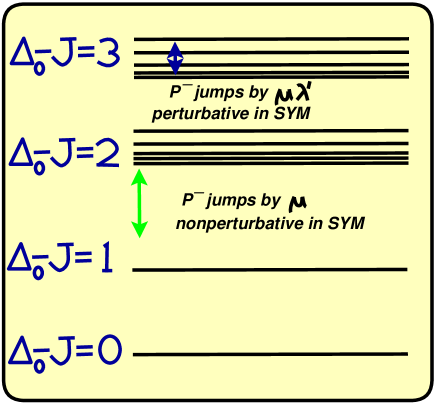
Figure 1: Hierarchy of energy scales for large $\mu p^{+}\alpha^{\prime}$. Only the transitions between states with the same $\Delta_{0}-J$, i.e. with the same number of impurities, can be calculated perturbatively. The big jumps change the energy by an amount $1/\lambda^{\prime}$ times bigger and therefore they result from non-perturbative effects in Yang-Mills theory.

Let us explain our proposal for string interactions in more detail. The spectrum of string states in the pp-wave background clumps into almost degenerate multiplets at large $\mu$. The splittings between states of the same multiplet are of order $\mu\lambda^{\prime}$, while the energy gap between distinct multiplets is of order $\mu$. In section 5 we propose that the matrix element of the light-cone Hamiltonian between single and double string states within the same multiplet is the three-point coefficient of the suitably normalized operator product coefficient of the corresponding operators (this quantity is ${\cal O}(g_{2})$), multiplied by the difference between their unperturbed light-cone energies. Since energy splittings within a multiplet are of order $\mu\lambda^{\prime}$, Hamiltonian matrix elements between such states are of order $\mu g_{2}\lambda^{\prime}$, corresponding to an invariant string coupling of order $g_{2}\sqrt{\lambda^{\prime}}$. For a class of BMN states we compute these matrix elements perturbatively in Yang-Mills theory. Note that transitions between states with different $\Delta_{0}-J$ involve large changes in energy; such transitions appear to be non-perturbative in the gauge theory (see figure 1).

In the paragraphs above we have presented a specific proposal relating interaction amplitudes in string theory with correlation functions of the dual gauge theory. In the next two paragraphs we describe the evidence in support of our proposal. As we describe below, our proposal passes a rather nontrivial consistency check. Further we have also partially verified our proposal by direct comparison of three point functions (computed in Yang-Mills perturbation theory) with three string light-cone matrix elements (computed using light-cone string field theory).

We first describe the consistency check on our proposal. In section 5 we compute the shift in dimension of a class of BMN operators to first order in $\lambda^{\prime}$ and first order in $g_{2}^{2}$, i.e. on the torus. We find that the anomalous dimensions receive non-zero corrections from the torus diagrams with a quartic interaction between “non-nearest neighbor” fields (see figure 10). The anomalous dimensions are proportional to $g_{2}^{2}\lambda^{\prime}$, the square of the effective string coupling, and are interpreted as mass renormalizations of excited string states. We then proceed to recompute the mass renormalization of excited string states using second-order quantum mechanical perturbation theory. We obtain the light-cone matrix elements needed for this computation from correlators computed in perturbative gauge theory, utilizing our prescription described above. These two independent computations agree exactly, constituting a highly nontrivial “unitarity” check on the consistency of our proposals.

In section five we also compare our proposal for string interactions with matrix elements of the light-cone Hamiltonian of string field theory. The light-cone Hamiltonian is generated by a two-derivative prefactor acting on a delta functional overlap. In section 5 we demonstrate that the three-point function of three BMN operators, computed in free Yang-Mills theory, reproduces the delta functional overlap between three string states at large $\mu$. We conjecture that, in the same limit, the prefactor of this delta functional overlap reproduces the second element of our formula for matrix elements (the difference between the unperturbed energies of the corresponding states). We sketch how string field theory predicts a modification of our prescription for the case of the operators involving $D_{\mu}Z$ and fermions.

We conclude this introduction with a digression that may help to put our work in perspective. Yang-Mills/String theory dualities have hitherto been understood, even qualitatively, only in regimes of strong gauge theory coupling. For instance, it has long been suspected that confining gauge theories may be reformulated as string theories, with tubes of gauge theory flux constituting the dual string. However, as flux tubes emerge at distance scales larger than $1/\Lambda_{QCD}$, their dynamics is nonperturbative in the gauge theory. More recently the Maldacena conjecture has established a duality between a conformal gauge theory (with a fixed line of couplings) and string theories on an $AdS$ background. However these dualities are well understood only at large values of the gauge coupling. In this paper, utilizing the BMN duality, we have taken the first steps in explicitly reformulating an effectively weakly coupled gauge theory as an interacting sting theory (IIB theory on the pp-wave background at large $\mu$). As perturbative gauge theories are under complete control, a detailed understanding of this extremely explicit duality holds the promise of significantly enhancing our understanding of gauge-string dualities in general.

The rest of this paper is organized as follows. Section 2 contains a review of subtle aspects of the BMN paper of importance to us. In section 3 we explain the counting that identifies $g_{2}=J^{2}/N$ as the genus counting parameter in free Yang-Mills. We also present the computation of planar three-point functions and torus two-point functions of BMN operators in free Yang-Mills theory. In section 4 we compute the torus contribution to the anomalous dimensions of BMN operators. In section 5 we present our proposals relating Yang-Mills computations to amplitudes of the string Hamiltonian. We also present a nontrivial unitarity check of our proposals, and compare our proposals to string field theory. In section 6 we conclude with a discussion of our results and directions for future work. The reader who is uninterested in the details of perturbative computations of Yang-Mills correlators can skip from section 3.1 to section 5. In Appendix A we present a precise definition of a class of BMN operators. In Appendix B we prove that D-terms interactions do not contribute to the correlation function computations presented in this paper. In Appendix C we present a rigorous and self-contained derivation of two point functions of BMN operators. In Appendix D we present an alternative method for Yang-Mills computations.

Note: As we were completing our manuscript, related papers appeared on the internet archive [9, 10, 11]. [9] overlaps with parts of sections three and four of our paper, while [10] overlaps with parts of section 3 and section 5.3 of this paper. Our results disagree with those of [9] and [10] in certain important respects. Unlike both of these papers we find non vanishing anomalous dimensions for BMN operators on the torus at first order in Yang-Mills coupling. We identify $g_{2}\sqrt{\lambda^{\prime}}$ rather than $g_{2}$ as the effective string coupling at large $\mu$. As noted above, we have presented a rather non-trivial unitarity check of our proposals. We have also compared our proposal for the three-string vertex with the Green-Schwarz string field theory [8].

2 Preliminaries

2.1 The BMN operators

The simplest single-trace operator with R-charge $J$ is

$$O^{J}=\frac{1}{\sqrt{JN^{J}}}\operatorname{Tr}Z^{J},$$ (2.7)

where

$$Z=\frac{X^{5}+iX^{6}}{\sqrt{2}}.$$ (2.8)

This is a chiral primary operator, with scaling dimension exactly equal to $J$ at all $\lambda^{\prime}$. According to the BMN proposal it corresponds to the light-cone ground state $|0,p^{+}\rangle$, where the map between parameters is given by (1.4).

Other protected operators may be generated from $O^{J}$ by acting on it with $SO(6)$, conformal, or supersymmetry lowering operators. For example, by acting on $O^{J+1}$ with a particular $SO(6)$ lowering operator yields

$$O^{J}_{0}=\frac{1}{\sqrt{N^{J+1}}}\operatorname{Tr}\left(\phi Z^{J}\right),$$ (2.9)

where we have defined the complex combinations of the scalars:

$$\phi=\frac{X^{1}+iX^{2}}{\sqrt{2}},\qquad\psi=\frac{X^{3}+iX^{4}}{\sqrt{2}}.\qquad$$ (2.10)

$O^{J}_{0}$ is chiral with scaling dimension $\Delta=\Delta_{0}=J+1$; it corresponds to the string state $a_{0}^{\phi{\dagger}}|0,p^{+}\rangle$, where $a_{0}^{\phi{\dagger}}=(a_{0}^{1{\dagger}}+ia_{0}^{2{\dagger}})/\sqrt{2}$. To take another example, $O^{J+2}$ acted on by two distinct $SO(6)$ lowering operators yields the protected operator

$$O^{J}_{n,-n}=\frac{1}{\sqrt{JN^{J+2}}}\sum_{l=0}^{J}\operatorname{Tr}\left(\phi Z^{l}\psi Z^{J-l}\right)$$ (2.11)

which corresponds to the BPS string state $a_{0}^{\psi{\dagger}}a_{0}^{\phi{\dagger}}|0,p^{+}\rangle$. Proceeding in this manner, all protected operators (operators dual to supergravity modes) of the Yang-Mills theory may be obtained by acting on $O^{J}$, for some $J$, with the appropriate number of lowering operators of various sorts.

As noted in the introduction, only protected operators remain in the spectrum as $N$ is taken to infinity with $g_{\text{YM}}^{2}$ held fixed, in any sector of fixed charge $J$. However when $J$ is taken to infinity together with $N$, it is possible to construct operators that are locally BPS. These operators consist of finite strings of fields (all of which are BPS) that are sewn together (in the trace) with varying phases into an operator of length $J\to\infty$ that is not precisely BPS. An example of such a near BPS operator is

$$O^{J}_{n,-n}=\frac{1}{\sqrt{JN^{J+2}}}\sum_{l=0}^{J}e^{2\pi inl/J}\operatorname{Tr}\left(\phi Z^{l}\psi Z^{J-l}\right)$$ (2.12)

We will usually abbreviate this as $O_{n}^{J}$; however we must be careful to distinguish between the two chiral operators $O_{0}^{J}$ and $O^{J}_{0,0}$. In an inspired guess, BMN conjectured that the operator $O_{n}^{J}$ corresponds to the string state $a^{\phi{\dagger}}_{n}a^{\psi{\dagger}}_{-n}|0,p^{+}\rangle$. As we have emphasized above, for $n\neq 0$ this operator is weakly non-chiral and its scaling dimension is corrected. However these corrections are finite, and may be expanded in a power series in $\lambda^{\prime}$ (this result follows to low orders from direct computation, but independently, to all orders by comparison with the exactly known string spectrum). Operators corresponding to more than two string oscillators acting on the vacuum are discussed in appendix A.

$O_{n}^{J}$ was obtained from $O^{J+2}$ by replacing two $Z$’s by the ‘impurities’ $\phi$ and $\psi$, and sprinkling in position dependent phases. The impurities $\phi$ and $\psi$ were obtained by the action of $SO(6)$ lowering operators on $Z$. In an analogous manner the impurity $D_{\mu}Z$ may be obtained by acting on $Z$ with the generators of conformal invariance. Similarly, supersymmetry operators acting on $Z$ produce gauginos. General BMN operators consist of these impurities sprinkled in a trace of $Z$’s, together with phases. For the purposes of this paper it will be sufficient to consider only scalar impurities, but we will explain in section 5 how our ideas can be extended and checked with the other types of impurities.

As we have stressed in the introduction, the dimensions of operators such as $O_{n}^{J}$ remain finite (and perturbatively computable at small $\lambda^{\prime}$) in the limit of infinite ’t Hooft coupling only because these operators differ very slightly from protected chiral operators. It is very important that the operator $O_{n}^{J}$ is defined to reduce precisely to the chiral operator $O_{0,0}^{J}$ when $n$ is set to zero. Even a small modification in the definition of this operator (such as a modification of the range of summation of the variable $l$ to $1,\dots,J$, as originally written in [2]) introduces a small—${\cal O}(1/\sqrt{J})$—projection onto operators that are far from chiral, resulting in perturbative contributions to scaling dimensions like $g_{\text{YM}}^{2}N/J$, which diverges in the BMN limit, and hence a breakdown of perturbation theory.

2.2 On the applicability of perturbation theory in the BMN limit

Consider the perturbative computation of, say, the planar scaling dimension $\Delta$ of a BMN operator such as $O_{n}^{J}$ in (2.12) above. Suppressing all dependence on $n$, the results of a perturbative computation may be organized (under mild assumptions) as

$$\Delta=\sum_{m=0}^{\infty}\left(\frac{g_{\text{YM}}^{2}N}{J^{2}}\right)^{m}f_{m}(g_{\text{YM}}^{2}N),$$ (2.13)

where $f_{m}$ are unknown functions of the ’t Hooft coupling. BMN computed the planar part of $f_{1}(0)$ using Yang-Mills perturbation theory, and deduced $f_{1}(\infty)$ using the duality to string theory on the pp-wave background. Quite remarkably they found that $f_{1}(0)=f_{1}(\infty)$. This result suggests that $f_{1}(x)$ is a constant function at the planar level. Recently, the authors of [11] have demonstrated that $f_{2}(0)=f_{2}(\infty)$, and have presented arguments which suggest that the planar components of $f_{m}(x)$ are constant functions for all $m$. Note that a term proportional to $x^{m}$ in $f_{m}(x)$ would result in the breakdown of perturbation theory, in the BMN limit, at order $(g_{\text{YM}}^{2}N)^{m+n}$. Consequently, the conjecture that $f_{m}(x)$ are constant functions for all $m$ is identical to the conjecture that $\lambda^{\prime}=g_{\text{YM}}^{2}N/J^{2}$ is the true perturbation parameter, for the computation under consideration, in the BMN limit.

In this paper we will proceed on the assumption that $\lambda^{\prime}$ is indeed the perturbative parameter for the computations we perform, namely low order calculations of non-planar anomalous dimensions and three-point functions of BMN operators. We will see that (2.13) acquires extra non-planar contributions proportional to $(J^{4}/N^{2})^{h}$ from genus $h$ diagrams. These contributions are finite in the BMN limit but they can be expanded in $\lambda^{\prime}$ just like (2.13). All our results are consistent with this conjecture, and lend it further support; however, it would certainly be interesting to understand this issue better.

3 Correlators in free Yang-Mills theory

3.1 Correlators of chiral operators at arbitrary genus

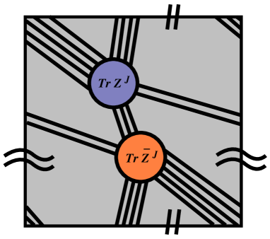
Figure 2: Genus one diagram drawn on a square.

Consider a correlation function involving operators of typical size (R-charge) $J$ in free $U(N)$ Yang-Mills theory. Following BMN, we study this correlator in the large $N$ limit; $J$ is simultaneously scaled to infinity with $J^{2}/N$ held fixed. In this section we will demonstrate that the number of graphs that contribute to this correlation function at genus $h$ scales with $J$ like $J^{4h}$. Since any particular genus $h$ graph is suppressed by a factor of $1/N^{2h}$ compared to a planar graph, we conclude that the net contribution of all genus $h$ graphs remains finite in the BMN limit, scaling like $g_{2}^{2h}$ where $g_{2}=J^{2}/N$. Consequently $g_{2}^{2}$ is a genus counting parameter; it determines the relative importance of higher genus graphs in free Yang-Mills theory.

The free Yang-Mills genus expansion encodes a modification in the dictionary between string states and Yang-Mills operators, but does not in itself appear to contain information about string interactions. We will return to the question of true string interactions in sections 4 and 5 below.

Consider the two-point function $\langle\bar{O}^{J}(0)O^{J}(x)\rangle$ in free Yang-Mills theory, where the operators $O^{J}$ are defined in (2.7). The planar contribution to this two-point function is

$$\langle\bar{O}^{J}(0)O^{J}(x)\rangle_{\text{planar}}=\frac{1}{(4\pi^{2}x^{2})^{J}}.$$ (3.14)

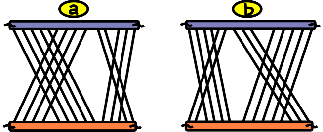
Figure 3: The same genus one diagram in an alternative representation. The diagram can be interpreted so that (a) the blue string $\operatorname{Tr}Z^{5+4+2+3}$ splits into $\operatorname{Tr}Z^{5+4}$ and $\operatorname{Tr}Z^{2+3}$; these two strings rotate by 5 or 2 units, respectively, to get the final state contracted with $\operatorname{Tr}\bar{Z}^{4+5+3+2}$. The same free theory diagram however also counts (b) a similar split of the string into $\operatorname{Tr}Z^{4+2}$ and $\operatorname{Tr}Z^{3+5}$.

To find the genus 1 contribution to the correlator, we must find all the free diagrams that can be drawn on the torus but not on the sphere. To do this the $J$ propagators must be divided into either 3 or 4 groups (see figure 2). The number of ways to do this is

$$\binom{J}{4}+\binom{J}{3}=\binom{J+1}{4}\approx\frac{J^{4}}{4!}.$$ (3.15)

This must be multiplied by $J$ for overall cyclic permutations, but then divided by $J$ again due to the normalization of the operator, and also by $N^{2}$ due to the genus. The resulting quantity is finite in the BMN limit, and proportional to $g_{2}^{2}$:

$$\langle\bar{O}^{J}(0)O^{J}(x)\rangle_{\text{torus}}=\frac{g_{2}^{2}}{4!(4\pi^{2}x^{2})^{J}}.$$ (3.16)

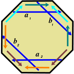
Figure 4: (a) Genus two surface represented as an octagon. The vertices of the octagon are all identified, while the edges are identified pairwise. The usual homology one-cycles with intersection numbers $\#(a_{i},b_{j})=\delta_{ij}$ are depicted.
(b) Genus two diagram. One operator is located at the center, and the other at the vertices. This way of drawing the diagram immediately generalizes to any genus.

This counting is easily extended to arbitrary genus. A genus $h$ Feynman graph can be drawn on a $4h$-gon with sides identified pairwise. As we see from figure 4, the number of graphs that can be drawn on a $4h$-gon is the number of ways of dividing $J$ lines into $4h$ groups, which is $J^{4h}/(4h)!$. (The lines may also be divided into $4h-1$ groups, but this gives a vanishing contribution in the BMN limit.) We must multiply this by the number of inequivalent ways of gluing the sides of a $4h$-gon into a genus $h$ surface. This number has been computed [51]; the result is

$${\frac{1\cdot 3\cdots(4h-1)}{2h+1}}.$$ (3.17)

Consequently a total of $2^{-2h}J^{4h}/(2h+1)!$ graphs contribute to this correlator at genus $h$. Summing over genera we find

$$\langle\bar{O}^{J}(0)O^{J}(x)\rangle=\frac{1}{(4\pi^{2}x^{2})^{J}}\sum_{h=0}^{\infty}\frac{1}{(2h+1)!}\left(\frac{g_{2}}{2}\right)^{2h}=\frac{2\sinh(g_{2}/2)}{g_{2}(4\pi^{2}x^{2})^{J}}.$$ (3.18)

This method can easily be generalized to show that the two-point function for an arbitrary chiral BMN operator such as $O^{J}_{0}$ or $O^{J}_{0,0}$ (defined in (2.9) and (2.12) respectively) has the same coefficient as in (3.18). Thus for example,

$$\langle\bar{O}^{J}_{0,0}(0)O^{J}_{0,0}(x)\rangle=\frac{2\sinh(g_{2}/2)}{g_{2}(4\pi^{2}x^{2})^{J+2}}.$$ (3.19)

The easiest way to generalize to higher-point functions of chiral operators is probably via a Gaussian matrix model. For example, it is not difficult to compute

$$\int{\cal D}Z\,{\cal D}{\bar{Z}}\left[\left(\prod_{i=1}^{k}\operatorname{Tr}Z^{J_{i}}\right)\operatorname{Tr}{\bar{Z}}^{J}e^{-\operatorname{Tr}(Z\bar{Z})}\right];\qquad\sum_{i=1}^{k}J_{i}=J$$ (3.20)

yielding simple explicit formulae that generalize (3.18).

3.2 Planar three-point functions

In this subsection we compute free planar three-point functions for the BMN operators defined in subsection 2.1. The results we obtain will be used in section 5 when we discuss the construction of string interactions.

We will first compute

$$\langle\bar{O}_{n}^{J}(0)O_{m}^{J_{1}}(x_{1})O^{J_{2}}(x_{2})\rangle,$$ (3.21)

where $J_{1}+J_{2}=J$. The planar, free field computation of this correlator is summarized in figure 12. The only complication is that we must sum over all of the possible positions for the $\phi$ and $\psi$ fields and carefully keep track of combinatorial factors as well as normalizations. The summation over the position of $\phi$ and $\psi$ in $O_{n}^{J_{1}}$ may be converted into integrals in the large $N$ limit,

$$J_{1}^{2}\int_{0}^{1}da\int_{0}^{1}db\,e^{2\pi ia(m-ny)}e^{-2\pi ib(m-ny)}=J_{1}^{2}\frac{\sin^{2}\pi ny}{\pi^{2}(ny-m)^{2}}.$$ (3.22)

where $y=J_{1}/J$. The final result for the correlator is obtained by multiplying this integral by $J_{2}$ (from cyclic rotations of $O^{J_{2}}$) and dividing by $\sqrt{J_{1}J_{2}J}$ (from the normalization of each operator) and by $N$ (from $1/N$ counting). We find

$$\langle{\bar{O}_{n}^{J}}(0)O_{m}^{J_{1}}(x_{1})O^{J_{2}}(x_{2})\rangle=\frac{g_{2}y^{3/2}\sqrt{1-y}\sin^{2}(\pi ny)}{\sqrt{J}\pi^{2}(ny-m)^{2}(4\pi^{2}x_{1}^{2})^{J_{1}+2}(4\pi^{2}x_{2}^{2})^{J_{2}}}.$$ (3.23)

A similar calculation yields

$$\langle\bar{O}_{n}^{J}(0)O_{0}^{J_{1}}(x_{1})O_{0}^{J_{2}}(x_{2})\rangle=\frac{g_{2}\sin^{2}(\pi ny)}{\sqrt{J}\pi^{2}n^{2}(4\pi^{2}x_{1}^{2})^{J_{1}+1}(4\pi^{2}x_{2}^{2})^{J_{2}+1}},$$ (3.24)

where $O_{0}^{J_{1}}$ and $O_{0}^{J_{2}}$ have $\phi$ and $\psi$ impurities respectively.

These expressions for the three-point functions will play an important role in our comparison between perturbative string theory and perturbative Yang-Mills theory in section 5.

3.3 Torus two-point functions of BMN operators

Figure 5: A typical free genus one graph for the two-point function of an operator with two impurities.

In this subsection we present an explicit computation of the two-point functions for the BMN operators (2.12) at genus one in free Yang-Mills theory. The operator $O^{J}_{n}$ differs from the chiral operator $O^{J}_{0,0}$ only in the presence of phases. Torus (and, indeed all genus) two point functions of $O^{J}_{0,0}$ were computed rather easily in (3.19). The additional phases complicates matters somewhat, as we will see below. Nonetheless, it is not difficult to convince oneself that these additional complications affect only the details of the result, but not its scalings with $J$ and $N$. Indeed, $g_{2}^{2}$ is the correct genus counting parameter for all free Yang-Mills computations in the BMN limit.

We consider first the correlator $\langle\bar{O}_{n}^{J}(0)O_{n}^{J}(x)\rangle$. The free genus one diagrams are given by the torus diagrams presented in the last section (figure 3) with $J+2$ lines, summed over all ways of replacing one line by a $\psi$ line and another by a $\phi$ line, with the rest becoming $Z$ lines. There are four groups of lines, and if the $\psi$ and $\phi$ are in different groups then their relative positions will be different in the first and second operators, giving a non-trivial phase (unlike in the case of planar diagrams where they are always the same distance apart in the first and second operators).

In fact it is convenient always to put the $\phi$ line at the beginning of both the first and second operator. With this convention every torus diagram with one $\phi$ line and $J+1$ other lines can be drawn as in figure 5, where each solid line represents a group of $Z$ lines, and $J_{1}+\dots+J_{5}=J+1$. Now we must put in the $\psi$ line. If it is in the first group ($J_{1}$ possibilities) or the last group ($J_{5}$ possibilities), then the phase associated with the diagram is 1, because it doesn’t move relative to the $\phi$ line. On the other hand if it’s in the second group ($J_{2}$ possibilities) then it moves to the right by $J_{3}+J_{4}$ steps, giving a phase $\exp(2\pi in(J_{3}+J_{4})/J)$. Similarly for the third and fourth groups, giving in all $J_{1}+J_{2}e^{2\pi in(J_{3}+J_{4})/J}+J_{3}e^{2\pi in(J_{4}-J_{2})/J}+J_{4}e^{-2\pi in(J_{2}+J_{3})/J}+J_{5}$. We must now sum this over all ways of dividing the $J+1$ lines into five groups:

$$\frac{(4\pi^{2}x^{2})^{J}}{g_{2}^{2}}\langle\bar{O}_{n}^{J}(0)O_{n}^{J}(x)\rangle_{\text{free torus}}$$

$$\qquad=\frac{1}{J^{5}}\sum_{\begin{subarray}{c}J_{1}+\dots+J_{5}\\ =J+1\end{subarray}}\left(J_{1}+J_{2}e^{2\pi in(J_{3}+J_{4})/J}+J_{3}e^{2\pi in(J_{4}-J_{2})/J}+J_{4}e^{-2\pi in(J_{2}+J_{3})/J}+J_{5}\right)$$

$$\qquad\xrightarrow[N\to\infty]{}\int_{0}^{1}\mathrm{d}j_{1}\cdots\mathrm{d}j_{5}\,\delta(j_{1}+\dots+j_{5}-1)$$

$$\qquad\qquad\times\left(j_{1}+j_{2}e^{2\pi in(j_{3}+j_{4})}+j_{3}e^{2\pi in(j_{4}-j_{2})}+j_{4}e^{-2\pi in(j_{2}+j_{3})}+j_{5}\right)$$

$$\qquad=\begin{cases}\frac{1}{24},&n=0,\\ \frac{1}{60}-\frac{1}{6(2\pi n)^{2}}+\frac{7}{(2\pi n)^{4}},&n\neq 0.\end{cases}$$ (3.25)

In taking the limit $N\to\infty$ the fractions $j_{i}=J_{i}/J$ go over to continuous variables.

If we now consider a correlator of two different operators $O_{n}^{J}$ and $O_{m}^{J}$, then the phase associated with a diagram depends not just on which group the $\psi$ is inserted into, but on where in the group it is inserted. The formulae are therefore somewhat more complicated, but it’s clear that again in the limit $N\to\infty$ the two-point function will reduce to $g_{2}^{2}$ times a finite integral:

$$\frac{(4\pi^{2}x^{2})^{J}}{g_{2}^{2}} \langle\bar{O}_{n}^{J}(0)O_{m}^{J}(x)\rangle_{\text{free torus}}\xrightarrow[N\to\infty]{}\int_{0}^{1}\frac{dj_{1}\cdots dj_{5}\,\delta(j_{1}+\dots+j_{5}-1)}{i(U-V)}\left(e^{i(U-V)j_{1}}-1\right.$$

$$\qquad\qquad\qquad\qquad\qquad\qquad\qquad\qquad{}+e^{iUj_{1}-iV(j_{1}+j_{3}+j_{4})}(e^{i(U-V)j_{2}}-1)$$

$$\qquad\qquad\qquad\qquad\qquad\qquad\qquad\qquad{}+e^{iU(j_{1}+j_{2})-iV(j_{1}+j_{4})}(e^{i(U-V)j_{3}}-1)$$

$$\qquad\qquad\qquad\qquad\qquad\qquad\qquad\qquad{}+e^{iU(j_{1}+j_{2}+j_{3})-iVj_{1}}(e^{i(U-V)j_{4}}-1)$$

$$\qquad\qquad\qquad\qquad\qquad\qquad\qquad\qquad{}+\left.e^{i(U-V)(j_{1}+j_{2}+j_{3}+j_{4})}(e^{i(U-V)j_{5}}-1)\right)$$

$$=\begin{cases}\frac{1}{24},&m=n=0;\\ 0,&m=0,n\neq 0{\text{ or }}n=0,m\neq 0;\\ \frac{1}{60}-\frac{1}{6U^{2}}+\frac{7}{U^{4}},&m=n\neq 0;\\ \frac{1}{4U^{2}}\left(\frac{1}{3}+\frac{35}{2U^{2}}\right),&m=-n\neq 0;\\ \frac{1}{(U-V)^{2}}\left(\frac{1}{3}+\frac{4}{V^{2}}+\frac{4}{U^{2}}-\frac{6}{UV}-\frac{2}{(U-V)^{2}}\right),&{\text{all other cases}}\end{cases}\!\!\!\!\!\!\!\!\!\!\!\!\!\!\!\!\!\!\!\!\!\!\!\!\!\!\!\!\!\!\!\!\!$$ (3.26)

Figure 6: A typical graph with nearest neighbor interaction. Four (blue) lines coming from the vertex should be replaced by all possible terms from figure 7. The dashed line is a $\psi$ propagator.

where $U=2\pi m,V=2\pi n$. The result for the free two-point function including genus one corrections can thus be summarized as

$$\langle\bar{O}_{n}^{J}(0)O_{m}^{J}(x)\rangle_{\text{free torus}}=\frac{\delta_{nm}+g^{2}_{2}A_{nm}}{(4\pi^{2}x^{2})^{J}},$$ (3.27)

where the entries for $A_{nm}$ are given above. As $\langle O^{J}_{n}\bar{O}^{J}_{n}\rangle$ is non-zero for $n\neq m$ (unless either $n$ or $m$ is zero), we see that $O^{J}_{n}$ and $O^{J}_{m}$ mix with each other, and that the mixing matrix elements are ${\cal O}(g_{2}^{2})$.

It is clear that the above procedure generalizes to the higher genus free diagrams described in section 2, in which the lines are divided into $4h$ groups. The genus $h$ contribution to the two point function may be written as $g_{2}^{2h}$ times a finite integral over $4h+1$ parameters. See appendix C for a rigorous, general discussion.

4 Anomalous dimensions from torus two-point functions

The planar anomalous dimension of the operator $O_{n}^{J}$ is related, via the duality with string theory, to the light-cone energy (or dispersion relation) of the corresponding free string state. The planar anomalous dimension was computed to first order in $g_{\text{YM}}^{2}$ in [2]. Their result was of order ${\cal O}(\lambda^{\prime}$), in precise agreement with the free spectrum of strings in the pp-wave background (1.3). On the other hand, the contribution to the anomalous dimensions from genus one gauge theory diagrams is related to the string one loop corrected dispersion relation for the corresponding state (see Section 5 for more details). In this section we compute the anomalous dimension of $O_{n}^{J}$ on the torus, to first order in $g_{\text{YM}}^{2}$. We find a result proportional to $g_{2}^{2}\lambda^{\prime}$, in accord with the identification of $g_{2}^{2}$ as the gauge theory genus counting parameter, and $\lambda^{\prime}$ as the effective gauge coupling. This result is a prediction for the one string loop ‘mass renormalization’ of the corresponding state.

Below we present a diagrammatic computation of this anomalous dimension; in appendices C and D two independent rigorous calculations confirm and generalize the results of this section.

We will find it convenient to think of the ${\cal N}=4$ Lagrangian in ${\cal N}=1$ language; $Z,\phi,\psi$ are the lowest components of the three adjoint chiral superfields of this theory. Most of the interactions of the theory, including scalar-gluon (and ghost) interactions and scalar-scalar interactions of the form $\operatorname{Tr}\left|[Z,\bar{\phi}]\right|^{2}$ are ‘flavor blind’ (see Appendix B). The contribution of these terms to this correlator is identical to their contribution to $\langle\operatorname{Tr}O^{J}\bar{O}^{J}\rangle$; consequently they vanish to order $g_{\text{YM}}^{2}$ by the theorem proved in [7] (see Appendix B for more details). Consequently, only flavor sensitive terms in the Lagrangian, i.e. F-terms, contribute to our calculation. The F-term interactions between scalars are very simple

$$V_{F}=-4g_{\text{YM}}^{2}\operatorname{Tr}\left(|[Z,\phi]|^{2}+|[Z,\psi]|^{2}+|[\phi,\psi]|^{2}\right).$$ (4.28)

Further, at the order under consideration, the last term does not contribute, as it is the square of a term anti-symmetric under $\phi\leftrightarrow\psi$ and so has vanishing Wick contractions with $O_{n}^{J}$ and its conjugate, as these operators are symmetric in $\phi$ and $\psi$. In summary, to the order under consideration, the two impurities do not talk to each other, and may be dealt with individually. Further, each impurity effectively only interacts quartically with the $Z$ fields through the interactions in (4.28).

We now turn to the computation of all diagrams with a single F-term interaction. Consider contributions to the two point function

$$\langle O^{J}_{n}(0)\bar{O}^{J}_{n}(x)\rangle.$$ (4.29)

from Feynman diagrams with a single $Z,\phi$ interaction vertex. All such graphs (see figure 6 for one example) have identical spacetime dependence and their Feynman integral is proportional to

$$\frac{1}{16\pi^{4}}\int\frac{d^{4}y}{y^{4}(y-x)^{4}}=\frac{\ln(\Lambda^{2}x^{2})}{8\pi^{2}x^{4}}.$$ (4.30)

We work in position space in (4.30); $y$ represents the position of the interaction point, which must be integrated over all space. The integrand in (4.30) consists of two propagators from $O^{J}_{n}(0)$ to the interaction point multiplied by two propagators from $\bar{O}^{J}_{n}(x)$ to the interaction point $y$, (see figures 6 and 2.7).

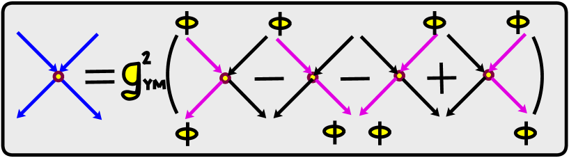
Figure 7: The quartic $Z$-$\phi$ vertices coming from the F-term (4.28).

In order to complete the computation of the torus two point function we must

• (a) Enumerate all graphs that can be drawn with a single F-term interaction on the torus.

• (b) Evaluate each of these graphs ignoring the propagators from the two operators to the interaction point (this corresponds to evaluating the corresponding free graph) and then multiply the result by (4.30).

• (c) Sum over the contribution from all these graphs.

In the rest of this section we carefully carry through this process to compute $\langle O^{J}_{n}(0)\bar{O}^{J}_{n}(x)\rangle$ on the torus, to first order in the Yang-Mills coupling. It turns out that the graphs that contribute may be categorized into three separate groups; nearest neighbor, semi-nearest neighbor, and non-nearest neighbor graphs, respectively.

4.1 Nearest neighbor interactions

Consider for example the diagram shown in figure 6, in which two adjacent lines in a free diagram such as figure 3 are brought together at an interaction vertex. We use the convention that diagrams at figure 6 actually represent the sum of four different Feynman diagrams. In diagrams such as figure 6, one of the lines connecting each of the operators to the interaction point is always $\phi$ propagator (two choices for each operator) and the other line always represents a $Z$ propagator. The four Feynman diagrams correspond to the four possible choices. The dashed line on the right in figure 6 represents a $\psi$ propagator. The four Feynman graphs that constitute the process depicted in figure 6 each contributes with the same weight; but graphs in which a $\phi$ line crosses the $Z$ line contribute with a relative minus sign (this follows from the fact that the interaction is derived from $g_{\text{YM}}^{2}\operatorname{Tr}\left|[Z,\phi]\right|^{2}$), as shown in figure 7. The total contribution of these four diagrams is thus

$$-\frac{g_{\text{YM}}^{2}}{N}(1-e^{2\pi in/J})(1-e^{-2\pi in/J})\approx-\frac{\lambda^{\prime}}{N^{2}}(2\pi)^{2}n^{2}$$ (4.31)

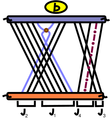
Figure 8: A typical graph with semi-nearest neighbor interaction.

times the phase associated to the corresponding free diagram. (4.31) is independent both of which two lines in the free diagram figure 3 we are considering. It also does not depend on which particular free diagram is under consideration. Consequently, the sum of all such “nearest-neighbor” diagrams is simply (4.31) multiplied by $A_{nn}$, the genus one contribution to the free correlator (3.27) calculated in the previous section (with an additional factor of two from diagrams in which the interaction involves the $\psi$ rather than the $\phi$ field).

Summing up all these diagrams, together with the free torus diagrams computed in this section, and adding these contributions to the free and one loop planar results computed in BMN we obtain the following correlator:

$$\langle\bar{O}_{n}^{J}(0)O_{n}^{J}(x)\rangle=\frac{1}{(4\pi^{2}x^{2})^{J+2}}\left(1-\lambda^{\prime}n^{2}\ln(\Lambda^{2}x^{2})\right)\left(1+g_{2}^{2}A_{nn}\right)+\cdots.$$ (4.32)

Consequently, the diagrams studied in this subsection merely correct the coefficient of the logarithm in the two point function to account for the changed normalization of the operator $O_{n}^{J}$, as computed in the previous section. If there were no further contributions to the coefficient of the logarithm, this result would imply that torus diagrams do not contribute to the anomalous dimensions of the BMN operators. In fact other diagrams we describe in the next two sections do modify the scaling dimensions, as we describe below.

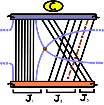
Figure 9: A typical graph with non-nearest neighbor interaction. Those graphs contribute to the actual anomalous dimension.

4.2 Semi-nearest neighbor interactions

There are two other classes of diagrams, illustrated in figures 8 and 9 (see also figure 10) that could potentially contribute to the correlator at order $g_{2}^{2}\lambda^{\prime}$, and thus to the anomalous dimension. As we will demonstrate below, the “semi-nearest-neighbor” diagrams of figure 8, in which the fields involved in the interaction are adjacent in one but not the other operator, contribute to the two point function $\langle O^{J}_{n}(0)\bar{O}^{J}_{m}(x)\rangle$ only when $m\neq n$. However, the “non-nearest neighbor” diagrams of figure 9 contribute to the logarithmic divergence of this correlator whether or not $n=m$. Consequently, these diagrams result in a genuine shift in the anomalous dimension of $O^{J}_{n}$.

It is not difficult to argue that no other classes of diagrams contribute to this process. To verify this claim, consider all diagrams with a single quartic interaction, that can be drawn on a torus. Each such diagram involves two propagator loops involving the interaction point. All diagrams fall into four classes; diagrams in which each of these loops is contractible, in which one loop is contractible and the other wraps a cycle of the torus, in which both loops wrap the same cycle of the torus, and finally those in which the two loops wrap different cycles of the torus. Further dressing these diagrams with all sets of propagators that leave it genus one, we find that the first class constitutes nearest neighbor graphs of the form figure 6, the second set constitutes semi-nearest neighbor graphs of the form figure 8, the third set constitutes nonnearest neighbor graphs of the form 9 and the last set cannot be implemented with F-term interactions. In Appendix C and D we verify this result using different techniques.

In this subsection we discuss the semi-nearest-neighbor diagrams. There are exactly eight diagrams of this type corresponding to the number of ways one may choose the last member of a given group in figure 8 to interact with the first member of the next group. The number of semi-nearest neighbor diagrams is smaller than the number of nearest neighbor diagrams by a factor of ${\cal O}(1/J)$ as either $\phi$ or $\psi$ must be located at the edge of one of the four ‘groups’ of lines in figure 8. Consequently such diagrams are naively negligible in the $J\to\infty$ limit. However, each individual semi-nearest neighbor diagram is enhanced by ${\cal O}(J)$ relative to a nearest neighbor diagram. In order to understand this, consider for example the case illustrated in figure 8. As in the previous case, this figure really represents four diagrams, which contribute a total

$$\frac{g_{\text{YM}}^{2}}{N}\frac{2\pi in}{J}\left(e^{2\pi inJ_{2}/J}-e^{-2\pi inJ_{1}/J}\right)e^{2\pi inJ_{3}/J}$$ (4.33)

(the last factor is due to the $\psi$ field, which in this particular example happens to sit in the fourth block, but whose position should be summed over). The fact that there is only one power of $J$ in the denominator, rather than two as in (4.31), compensates the fact that these diagrams are rarer by a factor of $1/J$ than the nearest-neighbor ones. Consequently, such diagrams could make non-vanishing contribution in the BMN limit $J\to\infty$, and they do contribute to $\langle O^{J}_{n}(0)\bar{O}^{J}_{m}(x)\rangle$ for $m\neq n$. However it turns out that the full contribution from semi-nearest neighbor graphs to the correlator above vanishes for the case $m=n$ considered in this section. One can see this either by considering the other semi-nearest neighbor diagrams at fixed $J_{1},J_{2},J_{3},J_{4}$ (there are 32 such diagrams in total), and seeing the cancellations explicitly, or by considering a fixed diagram such as figure 8 summed over $J_{1},J_{2},J_{3},J_{4}$—since (4.33) is antisymmetric under exchange of $J_{1}$ and $J_{2}$ it must vanish in the sum.

4.3 Non-nearest neighbor interactions

Finally, we turn to the non-nearest-neighbor graphs described in the figure 9 (redrawn differently in figure 10). The external legs of our operator are divided into three groups containing $J_{1}$ and $J_{2}$ or $J_{3}$ $Z$’s, respectively. Because we have divided the $Z$ propagators into three rather than four lines, these diagrams are rarer still by a factor $1/J$ than the semi-nearest-neighbor diagrams, or by a factor of ${\cal O}(1/J^{2})$ compared to nearest neighbor diagrams. However, this is compensated by the fact that each non-nearest neighbor diagram is enhanced by a factor ${\cal O}(J)$ compared to semi-nearest neighbor diagrams, or ${\cal O}(J^{2})$ compared to non-nearest neighbor diagrams. In order to see this note that in the diagram of figure 9 both ends of the $\phi$ propagator jump by a macroscopic (i.e. order $J$) distance along the string of $Z$’s. Let the impurity $\phi$ be located on the left and/or right end of the group $J_{1}$ whose first and last propagators are “pinched”. The four diagrams represented by figure 9 consequently contribute equally, but weighted by phase $1$, (for the two diagrams in which $\phi$ does not jump) or $-\exp(\pm 2\pi inJ_{1}/J)$ for the diagrams in which $\phi$ jumps either to the left/ right; consequently the sum of these four diagrams is proportional to

$$(1-e^{2\pi inJ_{1}/J})(1-e^{-2\pi inJ_{1}/J}).$$

Figure 10: Figure 9 represented as a periodic square.

We now turn to the contribution to the diagram from the phase associated with the second impurity $\psi$. If $\psi$ is in one of $J_{1}$ places inside the first vertical block its relative position on the two operators is the same, and so these $J_{1}$ diagrams contribute with no phase. On the other hand, if $\psi$ is in the block with $J_{2}$ propagators; its relative position on the two operators is different by $J_{3}$; the corresponding $J_{2}$ diagrams contribute with phase $\exp(2\pi inJ_{3}/J)$. Finally, if $\psi$ can be located in the third block (with $J_{3}$ propagators) its relative position on the two operators slides to the left by $J_{2}$ units. Consequently, these $J_{3}$ diagrams are each proportional to $\exp(-2\pi inJ_{2}/J)$. Replacing the sum over $J^{i}$ (with $J_{1}+J_{2}+J_{3}=J$) by an integral over $j_{i}=J_{i}/J$ (with $j_{1}+j_{2}+j_{3}=1$), we arrive at the integral

$$\int_{0}^{1}dj_{1}dj_{2}dj_{3}\,\delta(j_{1}+j_{2}+j_{3}-1)(j_{2}e^{2\pi inj_{3}}+j_{3}e^{-2\pi inj_{2}}+j_{1})|1-e^{2\pi inj_{1}}|^{2}=\frac{1}{3}+\frac{5}{2\pi^{2}n^{2}}$$ (4.34)

(for $n\neq 0$). The two-point function is thus, at first order in $\lambda^{\prime}$ and $g_{2}^{2}$, given by

$$(4\pi^{2}x^{2})^{J+2}\langle\bar{O}_{n}^{J}(0)O_{n}^{J}(x)\rangle=\\ (1+g_{2}^{2}A_{nn})\left(1-n^{2}\lambda^{\prime}\ln(\Lambda^{2}x^{2})\right)+\frac{\lambda^{\prime}g_{2}^{2}}{4\pi^{2}}\left(\frac{1}{3}+\frac{5}{2\pi^{2}n^{2}}\right)\ln(\Lambda^{2}x^{2}),$$ (4.35)

and the anomalous dimension is given by

$$\Delta=J+2+\lambda^{\prime}n^{2}-\frac{g_{2}^{2}\lambda^{\prime}}{4\pi^{2}}\left(\frac{1}{3}+\frac{5}{2\pi^{2}n^{2}}\right).$$ (4.36)

The methods described in this section, or the ones described in appendices C and D, may also be used to calculate the two-point function between different operators. We summarize the result here; the reader will find the details in the appendices:

$$(4\pi^{2}x^{2})^{J+2}\langle\bar{O}_{n}^{J}(0)O_{m}^{J}(x)\rangle=\\ (\delta_{nm}+g_{2}^{2}A_{nm})\left(1-(n^{2}-nm+m^{2})\lambda^{\prime}\ln(\Lambda^{2}x^{2})\right)+\frac{\lambda^{\prime}g_{2}^{2}}{4\pi^{2}}B_{nm}\ln(\Lambda^{2}x^{2}).$$ (4.37)

Here the first, factorized term contains the contributions of the nearest-neighbor (proportional to $nm$) and semi-nearest-neighbor (proportional to $(n-m)^{2}$) diagrams. The second term contains the contribution of the non-nearest-neighbor diagrams:

$$B_{nm}=\begin{cases}0,&n=0{\text{ or }}m=0;\\ \frac{1}{3}+\frac{10}{U^{2}},&n=m\neq 0;\\ -\frac{15}{2U^{2}},&n=-m\neq 0;\\ \frac{6}{UV}+\frac{2}{(U-V)^{2}},&{\text{all other cases,}}\end{cases}$$ (4.38)

where $U=2\pi m$ and $V=2\pi n$.

The classification of diagrams into nearest-, non-nearest-, and semi-nearest-neighbor continues to be valid at higher genus (at first order in $\lambda^{\prime}$). Interestingly, the factorization of the first two contributions, as in (4.37), is true at all genera.

5 String interactions from Yang-Mills correlators

In this section we finally turn to the relationship between correlation functions in Yang-Mills and dual string interactions. We make two specific proposals at large $\mu$:

• Three-point functions of suitably normalized BMN operators, multiplied by the difference in $p^{-}$ between the ingoing and outgoing operators, may be identified with the matrix elements of the light-cone Hamiltonian between the corresponding one string and two string states.

• The one string loop mass renormalization of a class of excited string states is reproduced by the ${\cal O}(g_{2}^{2})$ anomalous dimensions of the corresponding operators.

We believe that these proposals form part of a larger dictionary relating the Yang-Mills theory and the string theory; however we leave the determination of the rest of this dictionary to future work.

This section is organized as follows. In subsection 5.1 we motivate and explain our proposals in detail, and elaborate on some of their consequences. In the rest of this section we provide evidence for the validity of our proposals. In subsection 5.2 we demonstrate that our proposals pass a nontrivial self-consistency check. In subsection 5.3 we compare our proposals (together with the computations of Yang-Mills correlators in section 3 and 4) with the predictions of string field theory, and find substantial agreement.

5.1 Three-string light-cone interactions from Yang-Mills three-point functions

Let $O_{i}$, $O_{j}$, and $O_{k}$ represent three single-trace BMN operators, of $U(1)$ charges $J_{i}$, $J_{j}$, and $J_{k}$, and normalized so that

$$\langle\bar{O}_{i}(0)O_{j}(x)\rangle=\frac{\delta_{ij}}{(2\pi x)^{2\Delta_{i}}}$$ (5.39)

Let $|i^{\prime}\rangle$ represent the free single string states that correspond to these operators at zero bulk string coupling, normalized such that

$$\langle i^{\prime}|j^{\prime}\rangle=\delta_{ij}$$ (5.40)

Let

$$\langle\bar{O}_{i}(x_{i})O_{j}(x_{j})O_{k}(x_{k})\rangle_{\text{free planar}}=\frac{\delta_{J_{i},J_{j}+J_{k}}C_{ijk}}{(2\pi x_{ij})^{\Delta_{i}+\Delta_{j}-\Delta_{k}}(2\pi x_{ik})^{\Delta_{i}+\Delta_{k}-\Delta_{j}}(2\pi x_{jk})^{\Delta_{j}+\Delta_{k}-\Delta_{i}}}$$ (5.41)

The coefficients $C_{ijk}$ have been evaluated in (3.23) and (3.24). At small $\lambda^{\prime}$, we propose the following formula for the matrix element of the string field theory light-cone Hamiltonian

$$\langle i^{\prime}|P^{-}|j^{\prime}k^{\prime}\rangle=\mu(\Delta_{i}-\Delta_{j}-\Delta_{k})C_{ijk}.$$ (5.42)

(5.42) is expected only to apply to leading order in $\lambda^{\prime}$; we leave its generalization to finite $\lambda^{\prime}$ to future work.

Equation (5.42) is one of the central proposals of our paper. In sections 5.2 and 5.3 below we will provide rather strong evidence for its validity. Before proceeding to do so, however, we provide initial motivation for the proposal (5.42). Inner products of Yang-Mills states on $S^{3}$ (and so, presumably, states of the dual string theory) are related to correlation functions of the Euclidean Yang-Mills theory by the state operator map. Thus it is plausible that matrix elements of the string theory light-cone Hamiltonian are given by Yang-Mills correlators, dressed by a factor of linear homogeneity in $p^{-}$.

We now motivate the specific form of the dressing in (5.42). Yang-Mills correlators, correctly normalized (see below), are of order $g_{2}^{2}$. On the other hand, from section 4, torus mass renormalizations occur at order $\mu g_{2}^{2}\lambda^{\prime}$, and so go to zero when $\lambda^{\prime}$ is taken to zero at fixed $g_{2}$. Consequently, the dressing factor must go to zero as $\lambda^{\prime}$ is taken to zero; this suggests the specific form of the formula (5.42).

In the rest of this subsection we elaborate on the consequences of (5.42).

5.1.1 Scaling with $N$ and $J$

Note that $C_{ijk}$ scales like $J^{3/2}/N$ for the BMN operators under consideration. Further, in the large $\mu$ limit the energy splittings $(p_{1}^{-}+p_{2}^{-}-p_{3}^{-})$ are of order $\mu\lambda^{\prime}$. Consequently, the right-hand side of (5.42) scales like $\mu g_{2}\lambda^{\prime}/\sqrt{J}$. As $J$ is taken to infinity in the BMN limit, these matrix elements scale to zero, which is puzzling at first sight. Note, however, that the number of intermediate states (or final states) in any process scales like $J$; consequently (see subsection 5.2) the scaling of matrix elements is precisely correct to yield finite contributions to physical processes. Stated differently, the scaling of matrix elements like $\mu g_{2}\lambda^{\prime}/\sqrt{J}$ is merely a consequence of dealing with string states that are unit normalized. Switching to the more conventional delta function normalization for states

$$\langle i|j\rangle=p^{+}_{i}\delta(p^{+}_{i}-p^{+}_{j})=J_{i}\delta_{J_{i},J_{j}}$$ (5.44)

requires a rescaling of states

$${|i\rangle}=\sqrt{J_{i}}{|i^{\prime}\rangle}.$$ (5.45)

Light-cone Hamiltonian matrix elements may then be written as

$$\langle i|P^{-}|jk\rangle=\left[(p_{i}^{-}-p_{j}^{-}-p_{k}^{-})\sqrt{\frac{J_{j}J_{k}}{J_{i}}}C_{ijk}\right]p_{i}^{+}\delta(p_{i}^{+}-p_{j}^{+}-p^{+}_{k})$$ (5.46)

The term in the square bracket on the RHS of (5.46) is finite in the BMN limit and is of order $\mu g_{2}\lambda^{\prime}$.

5.1.2 Effective Coupling

It is instructive to perform the following exercise. Consider an effective two dimensional field theory with scalar fields $\phi_{i}$, interacting through a $p^{+}$ dependent cubic interaction

$$\propto\int dx^{+}dp_{i}^{+}dp_{j}^{+}dp_{k}^{+}g(p_{i}^{+},p_{j}^{+},p_{k}^{+})\delta(p_{i}^{+}+p_{j}^{+}-p_{k}^{+})\phi_{i}(x^{+},p_{i}^{+})\phi_{j}(x^{+},p_{j}^{+})\phi_{k}(x^{+},p_{k}^{+})$$ (5.47)

Canonically quantizing this theory in the light-cone, it is not difficult to verify (for example, by adapting equation (23) of [50] to our normalization) that the matrix elements for the light-cone Hamiltonian of this system are

$$\langle i|P^{-}|jk\rangle\propto\int dp_{i}^{+}dp_{j}^{+}dp_{k}^{+}g(p_{i}^{+},p_{j}^{+},p_{k}^{+})\delta(p_{i}^{+}+p_{j}^{+}-p_{k}^{+})$$ (5.48)

Consequently we conclude that (5.46) would be reproduced from a two dimensional cubic effective field theory with coupling (of dimension squared mass) given by $g(p_{i}^{+},p_{j}^{+},p_{k}^{+})=(p_{i}^{-}-p_{j}^{-}-p_{k}^{-})\sqrt{J_{j}J_{k}/J_{i}}\,C_{ijk}p_{i}^{+}$, i.e.

$$g(p_{1}^{+},p_{2}^{+},p_{3}^{+})\approx\frac{1}{\alpha^{\prime}}(\Delta^{1}+\Delta^{2}-\Delta^{3})\frac{\sqrt{J_{1}J_{2}J_{3}}}{\sqrt{gN}}C_{123}\sim\frac{{\cal O}(g_{2}\sqrt{\lambda^{\prime}})}{\alpha^{\prime}}$$ (5.49)

leading to the identification of $g_{2}\sqrt{\lambda^{\prime}}$ as the effective string coupling for these processes.

5.1.3 Vanishing of on-shell amplitudes

Recall that, in field theory, the decay of a particle is the result of the mixing between single particle states and multi particle states of the same energy. This mixing invalidates the use of non-degenerate perturbation theory in following the ‘evolution’ of the unperturbed single particle state upon turning on an interaction. It fuzzes out the very notion of a particle; in particular the mixing broadens out delta function peaks in spectral functions, endowing the ‘particle’ with a finite lifetime.

It is striking that (5.42) prescribes the vanishing of matrix elements of the light-cone Hamiltonian between states of equal unperturbed energy. This prescription implies the stability of excited string states in the large $\mu$ limit even upon turning on interactions. As the notion of a single particle continues to be well defined in the interacting theory, it is thus natural to identify the BMN operator (2.12) with the stable one-particle state, at large $\mu$, even upon turning on interactions. This feature (the vanishing of matrix elements between states of equal unperturbed energy) also permits the use of non-degenerate quantum mechanical perturbation theory in an analysis of mass renormalization of excited string states at large $\mu$. We will utilize this observation in subsection 5.2 below.

5.2 Unitarity check

As we argued in the introduction, eight transverse coordinates in the pp-wave background are effectively compactified. The light-like direction is also compact at finite $N$ (its conjugate momentum, $J$, is quantized) and string theory on the pp-wave background reduces to quantum mechanics. In this subsection, we apply standard quantum mechanical second order perturbation theory to perform a self-consistency check of the amplitudes calculated from the gauge theory. The Hamiltonian here is $\Delta=J+P^{-}/\mu$.

Consider the string state corresponding to the BMN operator $O_{n}^{J}$ defined in equation (2.12). We will use the well known formula for non-degenerate second order perturbation theory

$$E_{n}^{(2)}=\sum_{m\neq n}\frac{\left|V_{mn}\right|^{2}}{E_{n}^{(0)}-E_{m}^{(0)}}$$ (5.50)

to compute its second order energy shift.

In (5.50), the sum over states $m$ includes two types of intermediate states:

• (A) the two-string states with strings corresponding to $O_{m}^{J_{1}}$ and $O^{J_{2}}$ (these must be summed over the worldsheet momentum $m$). Using (5.42) and (3.23), the squared matrix element that connects $O_{n}^{J}$ to this two-particle state is

  $$|V_{mn}|^{2}=\frac{g_{2}^{2}\lambda^{\prime 2}(1-y)(ny+m)^{2}\sin^{4}(\pi ny)}{\pi^{4}Jy(ny-m)^{2}}$$ (5.51)

  where we have defined $y=J_{1}/J$. The difference in energies between our state and the two-particle state is

  $$E_{n}-E_{m}=\frac{\lambda^{\prime}(n^{2}y^{2}-m^{2})}{y^{2}}.$$ (5.52)

• (B) the two-string states described by the two chiral primaries $O_{0}^{J_{1}}$ and $O_{0}^{J_{2}}$, where the impurities are $\phi$ and $\psi$ in the two operators respectively. The squared matrix element of the light-cone Hamiltonian connecting $O_{n}^{J}$ to this two-particle state is easily computed from (5.42) and (3.24):

  $$|V_{n0}|^{2}=\frac{g_{2}^{2}\lambda^{\prime 2}\sin^{4}(\pi ny)}{\pi^{4}J}.$$ (5.53)

  The difference in unperturbed energies between the initial and intermediate states is $E_{n}=\lambda^{\prime}n^{2}$.

In both cases, we must sum over $J_{1}=J-J_{2}$, i.e. integrate over $y=J_{1}/J$ from $0$ to $1$.

The total torus correction to the dimension of $O^{J}_{n}$ is therefore

$$\Delta^{(2)}_{n}=J\int_{0}^{1}dy\left(B^{(n)}+\sum_{m\in\mathbb{Z}}A_{m}^{(n)}\right),$$ (5.54)

where

$$A_{m}^{(n)}\equiv\frac{\left|V_{mn}\right|^{2}}{E_{n}-E_{m}}=\frac{g_{2}^{2}\lambda^{\prime}y(1-y)(ny+m)\sin^{4}(\pi ny)}{\pi^{4}J(ny-m)^{3}}$$ (5.55)

and

$$B^{(n)}\equiv\frac{|{V_{n0}}|^{2}}{E_{n}-E_{m}}=\frac{4g_{2}^{2}\lambda^{\prime}\sin^{4}\pi ny}{\pi^{2}Jn^{2}}$$ (5.56)

The sum over $m$ in (5.54) may be performed using the identity

$$\sum_{m\in\mathbb{Z}}\frac{ny+m}{(ny-m)^{3}}=-\pi^{2}\csc^{2}(\pi ny)\left(1+2\pi ny\cot(\pi ny)\right).$$ (5.57)

Adding $B^{(n)}$ to the result and performing the integral over $y$, we find

$$\Delta^{(2)}_{n}=-\frac{g_{2}^{2}\lambda^{\prime}}{4\pi^{2}}\left(\frac{1}{3}+\frac{5}{2\pi^{2}n^{2}}\right),$$ (5.58)

which is precisely (4.36), the genus one contribution to the anomalous dimension.

In conclusion, we have computed the one loop mass renormalization from gauge theory in two different ways; from the genus one contribution to the anomalous dimension of the corresponding operator, and independently using our proposal (5.42) and standard second order perturbation theory. These two computations agree exactly. In the next subsection we will proceed to compare our prescription (5.42) with the predictions of string field theory.

Figure 11: A Feynman diagram for the planar three-string correlator and the corresponding light-cone gauge history of joining strings.

5.3 Comparison with string field theory

5.3.1 The delta-functional overlap

In this subsection we show that the free planar three-point function in Yang-Mills theory is identical to the delta-function overlap between string states in the large $\mu$ limit.

In the light-cone gauge, the bosonic part of the worldsheet action of a string propagating in the pp-wave background is

$$\frac{1}{4\pi{\alpha^{\prime}}}\int\left(\partial_{t}X^{i}\partial_{t}X^{i}-\partial_{\sigma}X^{i}\partial_{\sigma}X^{i}-\mu^{2}X^{i}X^{i}\right).$$ (5.59)

In the limit $\lambda^{\prime}\to 0$, at finite $n$ the sigma derivative piece in (5.59) ($\partial_{\sigma}X^{i}\partial_{\sigma}X^{i}$) is negligible compared to the mass term, and may simply be ignored, to zeroth approximation. It is convenient to discretize the worldsheet (5.59) into $J$ bits. On neglecting $\partial_{\sigma}X^{i}\partial_{\sigma}X^{i}$, the bits decouple from each other, and the string disintegrates into $J$ independent harmonic oscillators.

Now consider an interaction process involving three of these strings. String splitting/joining interactions in light-cone gauge are local, and the most important piece of the three-string interaction Hamiltonian is the overlap delta functional

$$\int{\cal D}X^{1}(\sigma){\cal D}X^{2}(\sigma){\cal D}X^{3}(\sigma)\,\Delta(X^{1}(\sigma)+X^{2}(\sigma)-X^{3}(\sigma))\psi(X^{1})\psi(X^{2})\psi^{*}(X^{3}).$$ (5.60)

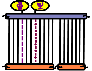
Figure 12: Three-point function in free theory as the delta functional overlap of the initial and final state.

On discretizing the three strings, every bit on the third string (the biggest of the three) is put in correspondence with a bit on one of the two smaller strings. Specifically, two bits are in correspondence if they share the same value of $\sigma$. The wave functions $\psi(X)$ factor into wave functions for each bit. Any bit is either in its harmonic oscillator ground state (we could denote that, in a diagram, by writing the letter $Z$ in the appropriate slot) or in the first excited state of $i^{\rm th}$ harmonic oscillator (denoted by $\phi^{i}$ in the appropriate slot). The interaction (5.60) is simply

$$\!\!\!\!\!\!\!\!\!\!\!\!\!\!\!\!\!\!\!\!\!\!\!\!\!\!\!\!\!\!\!\!\!\!\!\!\!\!\!\!\!\!\!\!\!\!\!\!\!\!\!\!\!\!\!\!\!\!\!\!V=\prod_{l}\langle\chi_{l}^{\prime}|\chi_{l}\rangle,$$ (5.61)

where the index $l$ runs over the bits of the larger string, $|\chi_{l}\rangle$ is the harmonic oscillator wave function of the $l^{\rm th}$ bit on the larger string, and $|\chi_{l}^{\prime}\rangle$ is the harmonic oscillator wave function on the corresponding bit on the corresponding smaller string (either string one or string two, depending on the value of $\sigma$). Diagrammatically, $V$ is unity when $Z$’s sit on top of $Z$’s and $\phi^{i}$s on top of $\phi^{i}$s. It is zero otherwise (see figure 12).

This is precisely the rule to compute the free planar contribution to the three-point function term by term in the series for the operators (2.5). The sum over phases in (2.5) is just the discrete Fourier series which may be taken simultaneously in Yang-Mills theory and on the discretized string world sheet. It is thus guaranteed that the results (3.10) and (3.11) from free planar gauge theory diagrams precisely reproduce the delta-functional overlap of strings in the $\mu\rightarrow\infty$ limit.

5.3.2 The prefactor

Our prescription (5.42) for the matrix elements of the light-cone Hamiltonian involved two elements.

• (a) The free Yang-Mills correlator.

• (b) The dressing factor $(p^{-}_{1}-p^{-}_{2}-p^{-}_{3})$.

Similarly, the one/two string light-cone Hamiltonian involves two elements, a delta function overlap, and a prefactor acting on that delta function overlap. In the previous subsection we have demonstrated that the delta function overlap is precisely equal to the free Yang-Mills correlator. In this subsection we conjecture that the action of the prefactor on this delta function precisely produces the dressing factor $(p^{-}_{1}-p^{-}_{2}-p^{-}_{3})$ multiplying the delta function overlap in (5.42).

The prefactor of string field theory involves two derivatives, and might naively have been estimated to be of order $p^{+}\mu$ at large $\mu$. In fact, as $\mu\to\infty$, the prefactor vanishes when acting on the delta functional overlap! This striking result is consistent with our proposal that the prefactor, acting on the delta functional produces a factor of

$$p^{-}_{1}-p^{-}_{2}-p^{-}_{3}={\cal O}(1/\mu)$$ (5.62)

An honest verification of (5.62) appears to be algebraically involved, though it is straightforward in principle.

A more detailed understanding of the structure of the string field theory prefactor in the large $\mu$ limit would permit several predictions for gauge theory correlators. For example, a preliminary analysis appears to indicate that the normalization of the prefactor (5.62) is proportional to the number of scalar impurities minus the number of $D_{\mu}Z$ impurities (with no contributions from fermionic impurities), and would seem to imply that the operators with one scalar and one $D_{\mu}Z$ excitation, as well as operators with fermionic excitations only, should have vanishing amplitudes.

6 Conclusions and outlook

In this paper we have begun an investigation into the relationship between Yang-Mills correlators in the BMN limit and string interactions in the pp-wave background. Our analysis is valid at large ${\alpha^{\prime}}p^{+}\mu\sim(\lambda^{\prime})^{-1/2}$ where the gauge theory appears effectively weakly coupled. We have employed perturbative Yang-Mills theory to make verifiable predictions for interaction amplitudes and mass renormalizations of weakly coupled strings on the pp-wave background.

The principal observations and proposals of our paper are

• For the appropriate class of questions, it appears that Yang-Mills perturbation theory in the BMN limit may be organized as a double expansion in an effective loop counting parameter $\lambda^{\prime}=g_{\text{YM}}^{2}N/J^{2}$ [2] and an effective genus counting parameter $g_{2}^{2}=J^{4}/N^{2}$. In particular, graphs of all genus continue to contribute, even in the strict ${\cal N}\to\infty$ BMN limit. The effective genus counting parameter $g_{2}^{2}$ may independently be identified as the two dimensional Newton’s constant for the dual string theory.

• Mixing effects between single and multi trace Yang-Mills operators are also controlled by the parameter $g_{2}$. This implies a modification of the dictionary between Yang-Mills operators and perturbative string states, proposed in [2] at the same order.

• We have proposed a relationship between Yang-Mills three point functions and three string interactions at large $\mu$. Our proposal, (5.42), implies that Light-cone Hamiltonian matrix elements between a wide class of single and double string states are of order $\mu g_{2}\lambda^{\prime}$, corresponding to invariant effective string coupling of order $g_{2}\sqrt{\lambda^{\prime}}$. At large values of this coupling string perturbation theory breaks down and string states blow up into giant gravitons. The detailed form of (5.42) also implies that, at large $\mu$, excited string states are stable, even at nonzero values of the effective string coupling.

• We have computed the one loop correction to the dispersion relation of these string states in two different ways: first by a direct computation of the anomalous dimension associated with this operator at order $g_{2}^{2}$ (i.e. on the torus), and second from quantum mechanical perturbation theory, using matrix elements obtained from three-point functions, as in the previous proposal. These computations agree exactly; this constitutes a non-trivial check on our proposals. They also confirm our identification of $g_{2}^{2}\lambda^{\prime}$ as the effective theoretic genus counting parameter.

This paper suggests several directions for future investigation. To begin with, it would be useful to check the proposals of this paper, and to better understand some its assumptions. It is very important to check our proposal for the dictionary between Yang-Mills correlators and string interactions; to this end an explicit expression for the first term in an expansion in powers of $1/\mu$ of the string field theory interaction vertex formally derived in [8] is required. It is certainly important to thoroughly understand when and why perturbative Yang-Mills can be employed in the study of this strongly interacting gauge theory (see [11]). Finally, in the unitarity check of section 5.2 we did not account for intermediate states with different numbers of impurities from those in the initial state. Contributions from such intermediate states are suppressed by large energy denominators. However, they could also be enhanced by parametrically large couplings. It would be useful to understand precisely when and why it is justified to omit such contributions.

Several generalizations of our work immediately suggest themselves. It should be straightforward to generalize our calculations and proposals to BMN operators involving $D_{\mu}Z$ and fermionic impurities. More generally, it would be very interesting to extend the dictionary between Yang-Mills and string theory proposed in this paper, beyond the large $\mu$ limit, and to wider classes of observables. It may also be possible to derive (5.42) and its generalizations from the more usual $AdS$/CFT prescriptions.

In conclusion, the BMN limit appears to allow us to re-interpret a sector of an effectively perturbative Yang-Mills theory as an interacting string theory! This remarkable idea certainly merits further study.

Appendix A Specification of operators

The operators of the ${\cal N}=~{}4~{}SYM$ theory which map into low-energy string states in the $pp$-wave background involve a large number $J$ of scalar fields $Z$ together with several impurity fields $\phi$ and $\psi$. It simplifies things to take these fields to be holomorphic combinations of the six real elementary scalars $X^{i}$ of the theory, e.g. $Z=(X^{5}+iX^{6})/\sqrt{2},\phi=(X^{1}+iX^{2})/\sqrt{2},\psi=(X^{3}+iX^{4})/\sqrt{2}$. We take $Z,\phi,\psi$ to be the lowest states of the three chiral multiplets $\Phi^{1},\Phi^{2},\Phi^{3}$ which appear in the ${\cal N}=1$ description of the ${\cal N}=4$ theory. BMN have outlined the rules for the construction of these operators, but there are some subtleties, and we thus briefly describe a clear specification here.

The principles of the construction are the following:

• (1) For the case of $I$ impurity fields there are $I$ initially independent phases $q_{j}=\exp(2\pi in_{j}/J)$. One writes a formal definition of the operators which reduces to a BPS operator when all $q_{i}=1$, specifically a “level $I$” $SU(4)$ descendent of the chiral primary operator $\operatorname{Tr}(Z^{J+I})$. Many of the operators so defined vanish; specifically they vanish unless the product $q_{1}q_{2}\cdots q_{I}=1$ which is the level-matching condition on string states.

• (2) On the “level-matching shell” the non-vanishing operators still satisfy the BPS property when all $q_{i}=1$. They reduce to the familiar BMN operator (with a minor but necessary change) for $k=2$ and extend the construction to general $k$. Planar diagrams for the 2-point correlation functions of these operators vanish (both for free fields and order $g_{YM}^{2}$ interactions) unless the momenta $n_{j}$ are conserved. This planar orthogonality property is approximate, holding to accuracy $1/J$ in the BMN limit $N\rightarrow\infty,J\sim\sqrt{N}$. Since the momenta do not have any clear meaning in the field theory, one should not expect strict momentum conservation. Indeed non-conservation becomes a leading effect for diagrams of genus $\geq 1$, again both for order $g_{YM}^{0}$ and order $g_{YM}^{2}$.

We start the discussion with the $I=2$ BMN operator

$$O_{J}=\sum_{l=0}^{J}q^{l}\operatorname{Tr}\left(\phi Z^{l}\psi Z^{J-l}\right),$$ (A.63)

modified so that the sum begins at $l=0$ rather than $l=1$ as in [2]. With this definition the BPS property is exact when $q=1$. This minor change is significant when one computes the planar correlator including interactions. For the operator defined above one finds by techniques described elsewhere in this paper that

$$\langle O_{J}(x)\bar{O}_{J}(0)\rangle=f_{J}(x)[1+cg_{YM}^{2}N(1-q)(1-\bar{r})\ln|x|]\sum_{l=0}^{J}(q\bar{r})^{l},$$ (A.64)

where $q=\exp(2\pi in/J)$ and $r=\exp(2\pi in^{\prime}/J)$ are the phases of the operators $O_{J}(x)$ and $\bar{O}_{J}(0)$, respectively, and $f_{J}(x)=(N/4\pi^{2}x^{2})^{J+2}$ involves the product of free scalar propagators. The factor $(1-q)(1-\bar{r})$ is the discrete second derivative of the phases coming from the stepping effect of the interactions noted in [2]. This factor contributes a $1/J^{2}$ suppression in the BMN limit. With the sum in the operator beginning at $l=1$ one would obtain a similar expression with the changes: a) the final sum in (A.64) starts at $l=1$, and b) there is an additional term proportional to $g_{YM}^{2}N(1+q\bar{r})\ln|x|$. The last term arises because the construction of discrete second derivative is incomplete at one site. It is not suppressed in the BMN limit. If present the physical interpretation would be spoiled, which is why is we chose the definition (A.63).

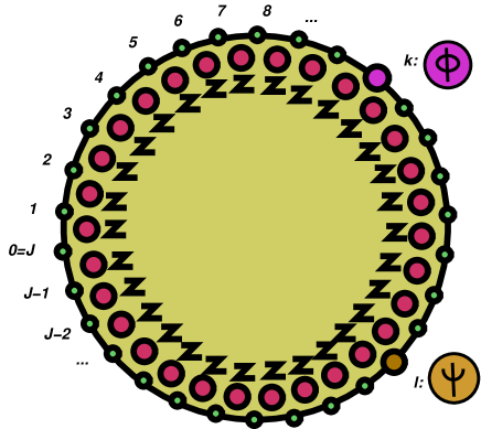
Figure 13: A circular array to indicate the $J$ $Z$-fields and the impurities $\phi,\psi$ at positions $k,l$ from a chosen origin.

The final sum in (A.63) has the value $J+1$ if $q\bar{r}=1$ and the value $1$ otherwise. In the BMN limit (to accuracy $1/J$) one thus obtains the momentum conserving result $J\delta_{n,n^{\prime}}$ as expected for a string in the state $a^{*}(n)b^{*}(-n)|0\rangle$ in the state dual to the operator $O_{J}$ in the limit $(\mu p^{+}\rightarrow\infty)$ when string interactions vanish.

The operator for two identical $\phi$ impurities is obtained simply by replacing $\psi$ by $\phi$ in (A.63). There are additional cross terms in the diagrams for the 2-point function. The planar result is just (A.64) with the final sum replaced by

$$\!\!\!\!\!\!\!\!\!\!\!\!\!\!\!\!\!\!\!\!\!\sum_{l=0}^{J}\left[(q\bar{r})^{l}+(qr)^{l}\right]=J\left(\delta_{n,n^{\prime}}+\delta_{n,-n^{\prime}}\right)$$ (A.65)

in the BMN limit. This is the correct orthogonality condition for (non-interacting) strings in the level-matched state $a^{*}(n)a^{*}(-n)|0\rangle$.

We now turn to the general program of defining operators off the “level-matching shell”. The general method is embodied in figure 13 which shows a circular array of $J$ points, the $J~{}Z$’s in the trace, with $\phi$ and $\psi$ in interstitial positions at distances $k$ and $l$ from an arbitrary origin. The associated phase is $q_{1}^{k}q_{2}^{l}$. It is clear from the figure that if we fix the relative distance, say $l$ between $\psi$ and $\phi$, and sum over rigid displacements of the positions of $\phi$ from $k=0$ to $k=J-1$, we accumulate the phase polynomial $q_{2}^{l}[1+q_{1}q_{2}+\cdots(q_{1}q_{2})^{J-1}]$ which vanishes unless the level-matching condition $n_{1}+n_{2}=0$ is obeyed.

The analytic expression for the operator depicted in figure 13 involves a sum over the two relative orders of $\phi,\psi$ within the trace. It is

$$O = O_{1}+O_{2};$$

$$O_{1} = \sum_{0\leq k\leq l\leq J-1}q_{1}^{k}q_{2}^{l}\operatorname{Tr}(Z^{k}\phi Z^{l-k}\psi Z^{J-l});$$

$$O_{2} = \sum_{0\leq l^{\prime}\leq k^{\prime}\leq J-1}q_{1}^{k^{\prime}}q_{2}^{l^{\prime}}\operatorname{Tr}(Z^{l^{\prime}}\psi Z^{k^{\prime}-l^{\prime}}\phi Z^{J-k^{\prime}}).$$ (A.66)

It is straightforward although a bit awkward to carry out analytically the sum over rigid displacements of a configuration of fixed relative phase $l$ pictured above. Cyclicity of the sum is vital, of course. Starting from $k=0$ in $O_{1}$ of (A.66) and moving to position $k=J-l-1$, one accumulates the phase polynomial $q_{2}^{l}[1+q_{1}q_{2}+\cdots(q_{1}q_{2})^{J-l-1}]$. The next step takes us into $O_{2}$ with $l^{\prime}=0,~{}k^{\prime}=J-l$, and we sum over $l^{\prime}$ in $l-1$ rigid steps until $\phi$ is in next-to-last position in the trace. The phase polynomial from this traversal of $O_{2}$ is $q_{1}^{J-l}[1+q_{1}q_{2}+\cdots(q_{1}q_{2})^{l-1}]$. The sum of these two polynomials is equal to the full polynomial in the previous paragraph, thus giving the level-matching condition exactly.

One may now impose the condition $q_{1}q_{2}=1$ and show that in non-vanishing cases the operator in (A.66) is just a factor of $J$ times that of (A.63). The first step is to substitute $q_{2}=1/q_{1}$ in $O_{1}$, and use the relative position index $a=l-k$ to rewrite the double-summed expression in (A.66) as

$$O_{1}=\sum_{a=0}^{J}(J-a)q_{2}^{a}\operatorname{Tr}(\phi Z^{a}\psi Z^{J-a}).$$ (A.67)

We have used the fact that, for fixed $a$, there are $J-a$ values of the original index $k$ which make identical contributions to $O_{1}$. The sum over $a$ in (A.67) actually stops at $a=J-1$, but it is useful to add the vanishing entry as we will see. The operator $O_{2}$ is handled similarly using $b=k^{\prime}-l^{\prime}$ as the relative phase index. By symmetry one finds

$$O_{2} = \sum_{b=0}^{J}(J-b)q_{1}^{b}\operatorname{Tr}(\psi Z^{b}\phi Z^{J-b})$$ (A.68)

$$= \sum_{a=0}^{J}aq_{2}^{a}\operatorname{Tr}(\phi Z^{a}\psi Z^{J-a}),$$

where we have redefined $a=J-b$, used cyclicity and $q_{1}=1/q_{2}$ in the last step. We see that the sum of (A.67) and (A.68) is equal to $J$ times the original on-shell operator (A.63) as claimed.

We have gone into considerable detail in the simple case of 2 impurities in order to avoid an impossibly awkward discussion in the general case which we now outline. In a set of $I\geq 3$ impurities, repetition of the fields $\phi,\psi$ occurs. However these fields are effectively distinguished in the construction of the operators because they carry different phases $q_{j}$. Wick contractions in the correlators will then impose Bose symmetry.

We therefore conceive of a set of $I$ independent impurity fields $\phi_{i},~{}i=1,\cdots I$, placed at arbitrary interstitial sites in the circle of figure 13, with assigned phase $q_{i}^{k_{i}}$. The analytic expression for the corresponding “off-level-matching-shell” operator is the sum $I!$ terms, one for each permutation of the impurities. The non-vanishing on-shell operator contains $(I-1)!$ terms including all non-cyclic permutations.

For $I=3$, the first of six terms can be written as

$$O_{1}=\sum_{0\leq k\leq l\leq m\leq J}q_{1}^{k}q_{2}^{l}q_{3}^{m}\operatorname{Tr}(Z^{k}\phi_{1}Z^{l-k}\phi_{2}Z^{m-l}\phi_{3}Z^{J-m}).$$ (A.69)

There are two similar terms, $O_{2},O_{3}$ for the cyclic permutations $(\phi_{2},\phi_{3},\phi_{1})$ and $(\phi_{3},\phi_{1},\phi_{2})$ of the impurity fields, and three more for anticyclic permutations. With due diligence one may repeat the argument above for the case $I=2$ and show that the sum $O_{1}+O_{2}+O_{3}$ vanishes unless the level-matching condition $q_{1}q_{2}q_{3}=1$ holds. The same property holds separately for the sum of the three operators for anti-cyclic permutations. The on-shell operator is the sum $O=O_{c}+O_{a}$ with the cyclic term

$$O_{c}=\sum_{0\leq a,\,\,0\leq b}^{a+b\leq J}q_{2}^{a}q_{3}^{a+b}\operatorname{Tr}(\phi_{1}Z^{a}\phi_{2}Z^{b}\phi_{3}Z^{J-a-b})$$ (A.70)

and an analogous expression $O_{a}$ for the anti-cyclic permutation $(\phi_{1},\phi_{3},\phi_{2})$, namely

$$O_{a}=\sum_{0\leq a,\,\,0\leq b}^{a+b\leq J}q_{3}^{a}q_{2}^{a+b}\operatorname{Tr}(\phi_{1}Z^{a}\phi_{3}Z^{b}\phi_{Z}^{J-a-b}).$$ (A.71)

With care, and with the $I=2$ case as a model, one can insert the on-shell condition $q_{1}=1/(q_{2}q_{3})$ in the operator $O_{1}$, introduce relative position indices $a=l-k,b=m-l$, and rewrite $O_{1}$ as

$$O_{1}=\sum_{0\leq a,\,\,0\leq b}^{a+b\leq J}(J-a-b)q_{2}^{a}q_{3}^{a+b}\operatorname{Tr}(\phi_{1}Z^{a}\phi_{2}Z^{b}\phi_{3}Z^{J-a-b}).$$ (A.72)

Cyclic symmetry implies similar expressions for $O_{2},O_{3}$, namely

$$O_{2} = \sum_{0\leq c,\,\,0\leq d}^{c+d\leq J}(J-c-d)q_{3}^{d}q_{1}^{c+d}\operatorname{Tr}(\phi_{2}Z^{c}\phi_{3}Z^{d}\phi_{1}Z^{J-c-d});$$

$$O_{3} = \sum_{0\leq e,\,\,0\leq f}^{e+f\leq J}(J-e-f)q_{1}^{e}q_{2}^{e+f}\operatorname{Tr}(\phi_{3}Z^{e}\phi_{1}Z^{f}\phi_{2}Z^{J-e-f}).$$ (A.73)

With the redefinitions $c=b,d=J-a-b,f=a,e=J-b-a$, creative use of the relation $q_{1}q_{2}q_{3}=1$, and cyclic symmetry, one may show that the sum $O_{1}+O_{2}+O_{3}=JO_{c}$. The analogous result relating the on-shell sum of three anti-cyclic permutations to $J$ copies of the anti-cyclic $O_{a}$ may be derived in the same way. This discussion shows that when the level matching condition holds, the off-shell operator for 3 impurities is just $J$ times the on-shell operator $O=O_{a}+O_{b}.$

The 2-point correlation function of the operator with $I=3$ impurities may be denoted by $\langle(O_{c}(x)+O_{a}(x))(\bar{O}_{c}(0)+\bar{O}_{a}(0))\rangle$. Planar diagrams come only from the diagonal terms $\langle O_{c}(x)\bar{O}_{c}(0)\rangle$ and $\langle O_{a}(x)\bar{O}_{a}(0)\rangle$. Contributions from both terms are required for planar orthogonality in the two independent momenta.

To order ${\cal O}(g_{YM}^{2})$ we obtain

$$\langle O(x)\bar{O}(0)\rangle = F(x)\left[1+g_{YM}^{2}NP(q_{i},r_{i})\ln|x|\right]\sum_{l=0}^{J}(q_{2}\bar{r}_{2})^{l}\sum_{m=0}^{J}(q_{3}\bar{r}_{3})^{m},$$ (A.74)

$$P(q_{i},r_{i}) = (1-q_{1}^{-1})(1-\bar{r}_{1}^{-1})+(1-q_{2})(1-\bar{r}_{2})+(1-q_{3})(1-\bar{r}_{3}).$$

$F(x)=(N/4\pi^{2}x^{2})^{J+3}$ is the product of $J+3$ scalar propagators and the corresponding color factor. $P(q_{i},r_{i})$ is of order $1/J^{2}$ exactly like the $O(g_{YM}^{2})$ expression for the two-point function of operators with two insertions (A.64). In the expression for $P(q_{i},r_{i})$ we have neglected higher order terms in $1/J$ that multiply terms of order $1/J^{2}$.

It is easy to understand how the structure of the interaction term arises. We are interested in planar contributions so we consider the nearest neighbor interactions only. The interactions can take place between any of the marked fields $\phi_{i}$ and the neighboring fields $Z$. The interaction in the conjugate operator $\bar{O}$ has to take place between the same marked field and neighboring fields $\bar{Z}$. Thus, we get the sum of three contributions with different phase dependence for each of the marked fields.

We hope that the discussion for $I=2,3$ impurities in this section makes the construction of the case of arbitrary $I$ clear.

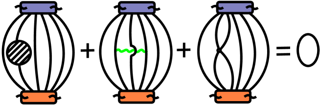
Figure 14: Cancellations at order $g_{YM}^{2}$.

Appendix B Irrelevance of D-terms

In this appendix we will show that the F-term interactions studied in the main text are the only interactions which need to be considered at order $g^{2}_{YM}$ in Yang-Mills perturbation theory. The sum of the other contributions, from D-terms, gluon exchange and self-energy insertions, precisely vanishes at this order in both 2- and 3-point functions (for an example see figures 14 and 15). This simple but useful fact can be proved by minor modifications of the techniques used for the same purpose in the studies of BPS operators in either [7] or [54]. We use the technique of [7].

We are concerned with the operators

$$O_{J}=\sum_{l=0}^{J}q^{l}\operatorname{Tr}\left(\phi Z^{l}\psi Z^{J-l}\right),$$ (B.75)

and we will show that the sum all non-F-term contributions vanishes term-by-term in the expansion in phases of $\langle O_{J}\bar{O}_{J}\rangle$ and $\langle O_{J}\bar{O}_{J_{1}}\operatorname{Tr}(\bar{Z}^{J_{2}})\rangle$.

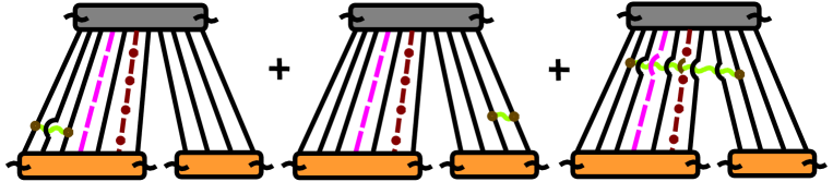
Figure 15: Gluon exchange contributions to a three-point function.

The first relevant observation comes from inspection of the form of the D-term potential in the ${\cal N}=4$ Lagrangian which is

$$V_{D}=g_{YM}^{2}\operatorname{Tr}\left([Z,\bar{Z}][Z,\bar{Z}]+2[\phi,\bar{\phi}][Z,\bar{Z}]+2[\psi,\bar{\psi}][Z,\bar{Z}]+2[\phi,\phi][\psi,\bar{\psi}]\right),$$ (B.76)

where we have dropped similar $\phi^{4}$ and $\psi^{4}$ terms which do not contribute to the correlators listed above. One now sees that all quartic vertices contribute to Feynman diagrams with the same combinatorial weight, independent of $SU(3)$ flavor. Similar remarks hold for gluon exchange diagrams. The 1-loop self-energy insertion is also flavor blind. Thus for the purposes of this Appendix, each summand in (A.63) can be replaced by $\operatorname{Tr}(Z^{J+2})$. One can now simply use the result of [7] which shows that all order $g_{YM}^{2}$ radiative corrections to $\langle\operatorname{Tr}(Z^{J+2})\bar{Z}^{J+2}\rangle$ cancel. Nevertheless, we will repeat the argument of [7] briefly because we will make a somewhat new application to 3-point functions below.

The first step is to observe that gluon exchange diagrams and those from $V_{D}\sim\operatorname{Tr}([Z,\bar{Z}]^{2})$ have the same color structure, and must be summed over all pairs of lines in the second Feynman diagram of figure 14. Self-energy insertions on each line must also be summed. The following identity holds for any set of matrices $M_{i},N$:

$$\sum_{i=1}^{n}\operatorname{Tr}\left(M_{1}\cdots[M_{i},N]\cdots M_{n}\right)=0.$$ (B.77)

Let $k=J+2$. Each diagram in figure 14 includes a sum over $k!$ permutations of the fields in $\operatorname{Tr}(\bar{Z}^{k})$ relative to a fixed permutation of the fields of $\operatorname{Tr}(Z^{k})$. Let $T^{a_{1}}\cdots T^{a_{k}}$ denote the fixed permutation of color generators of the fields in $\operatorname{Tr}(Z^{k})$, and let $T^{b_{1}}\cdots T^{b_{k}}$ denote one of the permutations of fields in $\operatorname{Tr}(\bar{Z}^{k})$. For each pair of fields $i\neq j$ the gluon exchange or D-term has a color structure which may be expressed as a commutator with the generators $T^{i}$ and $T^{j}$ in the product $T^{b_{1}}\cdots T^{b_{k}}$. Summing over all pairs, we obtain the net contribution

$$-B(x)\operatorname{Tr}(T^{a_{1}}\cdots T^{a_{k}})\sum_{i\neq j=1}^{k}\operatorname{Tr}(T^{b_{1}}\cdots[T^{b_{i}},T^{e}]\cdots[T^{b_{j}},T^{e}]\cdots T^{b_{k}}),$$ (B.78)

where $B(x)=b_{0}+b_{1}\ln(x^{2}M^{2})$ is the space-time factor associated with the interaction. We now use (B.77) on one of the commutators to rewrite (B.78) as

$$B(x)\operatorname{Tr}(T^{a_{1}}\cdots T^{a_{k}})\sum_{i=1}^{k}\operatorname{Tr}(T^{b_{1}}\cdots[[T^{b_{i}},T^{e}],T^{e}]\cdots T^{b_{k}})$$

$$=NB(x)\operatorname{Tr}(T^{a_{1}}\cdots T^{a_{k}})\sum_{i=1}^{k}\operatorname{Tr}(T^{b_{1}}\cdots T^{b_{i}}\cdots T^{b_{k}}).$$ (B.79)

In the last step we recognize $[[~{},T^{e}],T^{e}]$ as the $SU(N)$ Casimir operator in the adjoint representation which gives $[[T^{a},T^{e}],T^{e}]=NT^{a}$ for any generator. The final sum thus has $k$ identical terms. Each self energy insertion also contains the adjoint Casimir and has the form $NA(x)=N(a_{0}+a_{1}\ln(x^{2}M^{2}))$, and there are $k$ such terms. The sum of all diagrams in figure 14 is thus

$$kN(B(x)+A(x))\operatorname{Tr}(T^{a_{1}}\cdots T^{a_{k}})\operatorname{Tr}(T^{b_{1}}\cdots T^{b_{k}}),$$ (B.80)

which must be summed over all permutations $\{b_{i}=\sigma(a_{i}):~{}i=1\cdots k\}$ and finally contracted on pairwise identical color indices. All manipulations above are valid for the case $k=2$ which is known to satisfy a non-renormalization theorem. Hence $B+A=0$, and radiative corrections (other than from F-terms) cancel for all $k$. Figure 16 shows a D-term diagram which cancels with others despite the intuition that a gauge theory vertex at the string interaction point, i.e. the saddle point of the toroidal stringy diagram, should be significant.

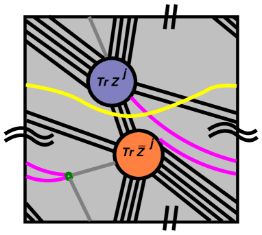
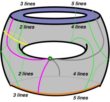
Figure 16: Two representations of a diagram which cancels with others.

Next we study the 3-point function $\langle O_{J}{\bar{O}_{J_{1}}}\operatorname{Tr}(\bar{Z}^{J_{2}})\rangle$ with $J=J_{1}+J_{2}$. The flavor blind property again means that the $JJ_{1}$ summands are all identical. Gluon exchange interactions among pairs of lines are indicated in figure 15. Quartic vertices from $V_{D}$ are similarly summed. We consider a fixed permutation of fields in $O_{J_{1}}$ and in $\operatorname{Tr}(Z^{J_{2}})$ and sum over permutations (i.e. orderings of generators $T^{c_{1}}\cdots T^{c_{J+2}}$) in the central operator $O_{J}$ and sum over permutations of fields from $O_{J_{1}}$ and from $\operatorname{Tr}(Z^{J_{2}})$. For interacting pairs which are connected to $O_{J_{1}}$ the previous argument applies mutatis mutandis. Radiative corrections cancel when self-energy insertions on $J_{1}$ lines are included. Idem for interacting pairs connected to $\operatorname{Tr}(Z^{J_{2}})$. The remaining pair interactions include one line connected to each operator. For these we use the color structure to place one commutator in each position in $\operatorname{Tr}(T^{a_{1}}\cdots T^{a_{J_{1}}})$ and one commutator in each position within $T^{b_{1}}\cdots T^{b_{J_{2}}}$. The resulting structure is then

$$C(x,y,z)\sum_{i=1,j=1}^{J_{1},J_{2}}\!\operatorname{Tr}(T^{a_{1}}\cdots[T^{i},T^{e}]\cdots T^{a_{J_{1}}})\,\operatorname{Tr}(T^{b_{1}}\cdots[T^{j},T^{e}]\cdots T^{b_{J_{2}}})\,\operatorname{Tr}(T^{c_{1}}\cdots T^{c_{J+2}}),$$ (B.81)

where $C(x,y,z)$ is a spacetime factor which need not be specified. However, for each fixed $i$, the sum on $j$ vanishes by (B.77), and our task is complete.

Appendix C Feynman diagrams and combinatorics

In this appendix we give a self-contained approach to the two-point correlation function discussed in the text. The purpose is to provide the detailed basis of results for planar and genus one contributions and to outline an algorithm to calculate genus $h>1$ results. We hope that the treatment below is readable both by physicists and mathematicians.

Let us summarize the results of this appendix. We show that genus $h$ two-point function in the free case is given by a sum of ${(4h-1)!!}/(2h+1)$ terms that correspond to the types of genus $h$ Feynman diagrams with $4h$ nonempty groups of edges. The two-point function with a single interaction equals $(2\pi)^{2}(nn^{\prime}+(n-n^{\prime})^{2})\times\textrm{(free case)}$ plus sum of $(4h-1)(4h-1)!!/[3(2h+1)]$ terms given by explicit formulas. The expression $(2\pi)^{2}nn^{\prime}\times\textrm{(free case)}$ comes from nearest neighbor interactions, the expression $(2\pi)^{2}(n-n^{\prime})^{2}\times\textrm{(free case)}$ comes from semi-nearest neighbor interactions, and the remaining expression comes from non-nearest neighbor interactions. The latter correspond to the types of genus $h$ diagrams with $4h-1$ nonempty groups of edges. For genus $h=1$, there is exactly one type of diagrams with 4 groups of edges, and there is one type of diagrams with 3 groups of edges. For genus $h=2$, there are 21 type of diagrams with 8 blocks and 49 types of diagrams with 7 blocks, etc.

It is natural to assume that, for 2 interactions, we need to go one level lower, i.e., the two-point function should be given by terms that depend on the free case and the single interaction case plus new additional part given by diagrams with $4h-2$ groups of edges, and so on for higher $h$. This gives a natural hierarchy of genus $h$ Feynman diagrams according to their numbers of blocks.

It is important to note that the notation used in this Appendix differs from that used in the main body of the paper in some respects. In subsections 3.3 and 4.2 of the main paper we have used the symbols $U=2\pi m$ and $V=2\pi n$ to parameterize the phases $e^{iU}$ and ^iV in BMN operators. In this appendix, we will usually use the symbols $u,v$ for these quantities. The indices $n,m$ will be denoted $n,n^{\prime}$. The symbol $A_{n,n^{\prime}}$ used repeatedly in sections 3 and 4 of the main body of the paper is identical to the symbol $A^{1}(n,n^{\prime})$ in this appendix. Finally, the contribution of non-nearest interactions denoted $B_{nm}$ in (4.37) is identical to $G^{1}_{\textrm{nn}}(n,n^{\prime})$ in the appendix.

C.1 Correlation functions

For a positive integer $J$ and two integers $n$ and $n^{\prime}$, the operators $O^{J}_{n}$ and $\bar{O}^{J}_{n^{\prime}}$ are given by

$$O_{n}^{J}=\sum_{l=0}^{J}q^{l}\operatorname{Tr}(\phi Z^{l}\psi Z^{J-l})\quad\textrm{and}\quad\bar{O}_{n^{\prime}}^{J}=\sum_{l^{\prime}=0}^{J}{\bar{r}}^{l^{\prime}}\operatorname{Tr}(\bar{Z}^{l^{\prime}}\bar{\psi}\bar{Z}^{J-l^{\prime}}\bar{\phi})\,,$$ (C.82)

where $q=\exp(2\pi in/J)$ and $r=\exp(2\pi in^{\prime}/J)$. (Here $i=\sqrt{-1}$). All fields $Z$, $\bar{Z}$, $\phi$, $\bar{\phi}$, $\psi$, $\bar{\psi}$ are given by $N\times N$ Hermitian matrices. We will discuss the free two-point correlation function:

$$\langle O_{n}^{J}(x)\,\bar{O}_{n^{\prime}}^{J}(y)\rangle=(4\pi^{2}(x-y)^{2})^{-J-2}\,A_{J,N}(n,n^{\prime})$$ (C.83)

and the two-point function with one interaction:

$$\langle O_{n}^{J}(x)\,[Z,\psi]\,[\bar{Z},\bar{\psi}]\,\bar{O}_{n^{\prime}}^{J}(y)\rangle=-\frac{g^{2}N\ln|x-y|}{2\pi^{2}}\,G_{J,N}(n,n^{\prime}).$$ (C.84)

The functions $A_{J,N}$ and $G_{J,N}$ can be written as series in powers of $N$:

$$A_{J,N}=N^{J+2}\sum_{h\geq 0}N^{-2h}\,A_{J}^{h}\qquad\textrm{and}\qquad G_{J,N}=N^{J+3}\sum_{h\geq 0}N^{-2h}\,G_{J}^{h}.$$ (C.85)

This is called the genus expansion of correlation functions, because $A_{J}^{h}$ and $G_{J}^{h}$ are given by sums over Feynman diagrams of some type drawn on an oriented genus $h$ surface.

As we will see, $A_{J}^{h}$ is of order $J^{4h+1}$ and $G_{J}^{h}$ is of order $J^{4h-1}$ as $J\to\infty$. Let

$$A^{h}(n,n^{\prime})=\lim_{J\to\infty}A_{J}^{h}/J^{4h+1}\qquad\textrm{and}\qquad G^{h}(n,n^{\prime})=\lim_{J\to\infty}G_{J}^{h}/J^{4h-1}\,.$$ (C.86)

The limits $A(g_{2};n,n^{\prime})=\lim A_{J,N}/(J\cdot N^{J+2})$ and $B(g_{2};n,n^{\prime})=\lim G_{J,N}/(J^{-1}\cdot N^{J+3})$, where $J,N\to\infty$ so that $J^{2}\sim g_{2}N$ for a fixed constant $g_{2}$, can be written as

$$A(g_{2};n,n^{\prime})=\sum_{h\geq 0}(g_{2})^{2h}\,A^{h}(n,n^{\prime})\qquad\textrm{and}\qquad G(g_{2};n,n^{\prime})=\sum_{h\geq 0}(g_{2})^{2h}\,G^{h}(n,n^{\prime}).$$ (C.87)

For any integer values of $n$ and $n^{\prime}$, $A(g_{2};n,n^{\prime})$ and $B(g_{2};n,n^{\prime})$ are analytic functions of $g_{2}$. In particular,

$$\begin{array}[]{l}\displaystyle A(g_{2};0,0)=\frac{2\sinh(g_{2}/2)}{g_{2}},\\[7.22743pt] A(g_{2};n,0)=A(g_{2};0,n^{\prime})=G(g_{2};0,0)=G(g_{2};n,0)=G(g_{2};0,n^{\prime})=0,\end{array}$$ (C.88)

for $n,n^{\prime}\neq 0$. We will see that

$$\begin{array}[]{l}A^{h}(n,n^{\prime})=\textrm{ sum of \ }(4h+1)\cdot\frac{(4h-1)!!}{2h+1}\textrm{ \ integrals},\\[10.84006pt] G^{h}(n,n^{\prime})=(2\pi)^{2}\cdot(-nn^{\prime}+(n-n^{\prime})^{2})\cdot A^{h}(n,n^{\prime})+G^{h}_{\mathrm{nn}}(n,n^{\prime}),\\[10.84006pt] \textrm{where \ }G^{h}_{\mathrm{nn}}(n,n^{\prime})=\textrm{ sum of \ }4\cdot(4h-1)\cdot\frac{(4h-1)!!}{2h+1}\textrm{ \ integrals}.\end{array}$$ (C.89)

Each of these integrals is given by an explicit formula. As an example, we will present closed formulas for $A^{h}(n,n^{\prime})$ and $G^{h}(n,n^{\prime})$ for small values of genus $h$. In general, the expressions for $A^{h}(n,n^{\prime})$ and $G^{h}(n,n^{\prime})$ have the form

$$\frac{\textrm{polynomial in $n$ and $n^{\prime}$}}{(n\cdot n^{\prime})^{a}\cdot(n-n^{\prime})^{b}\cdot(n+n^{\prime})^{c}}.$$ (C.90)

C.2 Free two-point function via permutations

Feynman diagrams for the free two-point function are basically given by permutations.

Let us recall a few basic facts about permutations. A permutation of order $m$ is a bijective map $w:\{1,\dots,m\}\to\{1,\dots,m\}$. Multiplication of permutations is given by composition of maps. All permutations of order $m$ form the symmetric group $S_{m}$. A cycle in a permutation $w$ is a subset of the form $\{w(i),w^{2}(i),\dots,w^{r}(i)=i\}$. In particular, each fixed point $w(i)=i$ is a cycle of size 1. Thus each permutation gives a decomposition of $\{1,\dots,m\}$ into a disjoint union of cycles. The number of cycles of $w$ is the total number of cycles in this decomposition. Let the long cycle $c\in S_{m}$ be the permutation that consists of a single $m$-cycle given by $c:i\mapsto i+1\pmod{m}$.

Feynman diagrams that describe Wick couplings in the free case $\langle O_{n}^{J}(x)\,\bar{O}_{n^{\prime}}^{J}(y)\rangle$ are given by permutations $w$ of order $m=J+2$ corresponding to mappings between the fields in $O_{n}^{J}(x)$ and the fields in $\bar{O}_{n^{\prime}}^{J}(y)$. The diagram with permutation $w$ produces a term with some power $N^{C(w)}$ of the rank $N$ of the gauge group $U(N)$. The exponent $C(w)$ is related to the genus $h(w)$ of the corresponding diagram by Euler’s formula:

$$C(w)=m-2\,h(w).$$ (C.91)

In physics language, $C(w)$ is the number of closed quark loops in the ribbonized diagram (a.k.a. fat graph) corresponding to the Feynman diagram with $U(N)$ adjoint fields. Combinatorially, $C(w)$ is the number of cycles in the twisted permutation $c^{-1}w^{-1}cw\in S_{m}$, where $c$ is the long cycle in $S_{m}$. The expression $A_{J,N}$, which gives the free two-point function, can be written as the following polynomial in the variables $q$, ${\bar{r}}$, and $N$

$$A_{J,N}=\sum_{w\in S_{m},\,w(1)=1}N^{C(w)}\,\sum_{i\geq 2}^{m}q^{i-2}{\bar{r}}^{w(i)-2}\,,$$ (C.92)

where the sum is over all permutations $w$ such that $w(1)=1$ (the first marked field $\phi$ is always contracted with $\bar{\phi}$), and the product is over all $i\neq 1$ (choice of position of the second marked field $\psi$).

Let us say that the number $h(w)=(m-C(w))/2$ is the genus of a permutation $w\in S_{m}$. It is always a nonnegative integer because the parity of the number $C(w)$ of cycles in the twisted permutation $c^{-1}w^{-1}cw$ is the same as the parity of $m$. Clearly, the genus of any cyclic shift $wc^{r}$ of $w$ is the same as the genus of $w$. Thus without loss of generality we will assume that $w(1)=1$. The $h$-th term $A^{h}_{J}$ in the genus expansion of $A_{J,N}$ is given by the terms in (C.92) with $w$ of given genus $h$. Since the only genus $0$ permutations are the identity permutation and its cyclic shifts, we have

$$A_{J}^{0}=(q{\bar{r}})^{0}+(q{\bar{r}})^{1}+\cdots+(q{\bar{r}})^{J}.$$ (C.93)

In the next section we will show that $A_{J}^{h}$ is a polynomial in $q$ and ${\bar{r}}$ given by a sum of order $J^{4h+1}$ terms $q^{i}{\bar{r}}^{j}$.

C.3 Block-reduction of permutations

For large values of $J$, the expression (C.92) involves a summation over permutations of large orders. This makes it difficult to calculate the limit $J\to\infty$ of this expression. Nevertheless it is possible reduce a permutation $w$ of arbitrary large order $m$ and small genus $h$ to a permutation $\sigma$ of order $\leq 4h$. The permutation $\sigma$ is the block-reduction of $w$ and is formally defined below.

For a permutation $w\in S_{m}$ with $w(1)=1$, let us subdivide the set $\{1,\dots,m\}$ into blocks as follows. If there are consecutive indices $i,i+1,\dots,i+k$ in the cyclic order such that $w(i)=j,w(i+1)=j+1,\dots,w(i+k)=j+k$ then we combine the indices $i,i+1,\dots,i+k$ into a single block. Here all indices $i$ and values $w(i)$ are understood modulo $m$. We will choose the blocks to be as maximal as possible. Thus the permutation $w$ gives a subdivision of the set $\{1,\dots,m\}$ into disjoint union of blocks $B_{1},\dots,B_{k}$ (where $1\in B_{1}$) formed by cyclically consecutive elements and a permutation $\sigma\in S_{k}$ of blocks. We call the permutation $\sigma$ the block-reduction of $w$. A permutation $\sigma\in S_{k}$, $k\geq 2$, is a block-reduction for some $w$ if and only if

$$\sigma(1)=1;\qquad\sigma(i+1)\neq\sigma(i)+1,\quad\textrm{for }i=1,\dots,k-1;\quad\textrm{and}\quad\sigma(k)\neq k.$$ (C.94)

Let us say that a permutation $\sigma\in S_{k}$ is block-reduced if it satisfies these conditions; and let $\mathrm{BR}_{k}^{h}$ be the set of block-reduced permutations of order $k$ and genus $h$. We will assume that $\mathrm{BR}_{0}^{0}$ contains one element—the empty permutation $\emptyset$ of order 0—which is the block-reduction of the identity permutation of any order.

Figure 17 shows two genus $h=1$ Feynman diagrams given by permutations $1\,2\,5\,6\,7\,3\,4\,8\,9\,10$ and $1\,2\,9\,10\,6\,7\,8\,3\,4\,5\,11\,12$. The first permutation has 3 blocks $B_{1}=\{8,9,10,1,2\}$, $B_{2}=\{3,4,5\}$, $B_{3}=\{6,7\}$ and its block-reduction is $1\,3\,2$. The second permutation has 4 blocks $B_{1}=\{11,12,1,2\}$, $B_{2}=\{3,4\}$, $B_{3}=\{5,6,7\}$, $B_{4}=\{8,9,10\}$ and its block-reduction is $1\,4\,3\,2$.

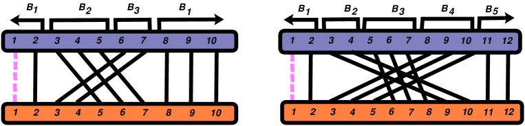
Figure 17: Two genus 1 permutations with block-reductions (a) $1\,3\,2$ and (b) $1\,4\,3\,2$.

Lemma C.1

A permutation $w$ and its block-reduction $\sigma$ have exactly the same genera $h(w)=h(\sigma)$. For each block-reduced permutation $\sigma\in S_{k}$ of genus $h$, we have $k\leq 4h$.

Proof —  Recall that genus of $w$ was defined in terms of the twisted permutation $\tilde{w}=c^{-1}w^{-1}cw$. The similar twisted permutation $\tilde{\sigma}$ for the block-reduction $\sigma$ of $w$ is obtained from $\tilde{w}$ by removing all its fixed points. Thus $\sigma$ and $w$ have same genera. Also, $\tilde{\sigma}\in S_{k}$ is a fixed-point free permutation. Thus its number of cycles is $C(\sigma)\leq k/2$ and the genus of $\sigma$ is $h(\sigma)=(k-C(\sigma))/2\geq k/4$. $\square$

There is only one genus 0 block-reduced permutation $\emptyset$ and two genus 1 block-reduced permutations 132 and 1432. For genus 2, there are 21 elements in $\mathrm{BR}_{8}^{2}$ and 49 elements in $\mathrm{BR}_{7}^{2}$. In general, the following statement holds.

Proposition C.2

For $h\geq 1$, the numbers of elements in $\mathrm{BR}_{4h}^{h}$ and in $\mathrm{BR}_{4h-1}^{h}$ are given by

$$|\mathrm{BR}_{4h}^{h}|=\frac{(4h-1)!!}{2h+1}\qquad\textrm{and}\qquad|\mathrm{BR}_{4h-1}^{h}|=\frac{4h-1}{3}\cdot|\mathrm{BR}_{4h}^{h}|.$$ (C.95)

Proof —  Elements of the set $\mathrm{BR}_{4h}^{h}$ are in one-to-one correspondence with gluing of the $4h$-gon into a genus $h$ surface. An element $\sigma\in\mathrm{BR}_{4h}^{h}$ is determined by its twist $\tilde{\sigma}=c^{-1}\sigma^{-1}c\sigma\in S_{4h}$, where $c$ is the long cycle in $S_{4h}$. The permutation $\tilde{\sigma}$ is a fixed-point free permutation with $2h$ cycles. Thus $\tilde{\sigma}$ is given by the product of $2h$ commuting transpositions. Let us label the sides of the $4h$-gon by the numbers $1,\dots,4h$ (in the clockwise order) and glue the side labelled $i$ with the side labelled $\tilde{\sigma}(i)$, for $i=1,\dots,4h$. This will produce a genus $h$ surface.

The numbers of gluings of any $2k$-gon into a genus $h$ surface were calculated by Harer and Zagier [51]. In the case $k=2h$, their result implies the number of gluings is $(4h-1)!!/(2h+1)$.

For $\sigma^{\prime}\in\mathrm{BR}_{4h-1}^{h}$, the twist $\tilde{\sigma}^{\prime}\in S_{4h-1}$ should be a permutation given by the product of $2h-2$ commuting transpositions and a single 3-cycle. Such $\tilde{\sigma}^{\prime}$ can be obtained from $\tilde{\sigma}$, for $\sigma\in\mathrm{BR}_{4h}^{h}$, by merging the first vertex $1$ with the last vertex $4h$ and replacing 2 transpositions $(1,\tilde{\sigma}(1))$ and $(4h,\tilde{\sigma}(4h))$ with a single 3-cycle $(1,\tilde{\sigma}(4h),\tilde{\sigma}(1))$. We will get all $\tilde{\sigma}^{\prime}$ such that the vertex 1 belongs to the 3-cycle. In order to get all possible $\tilde{\sigma}^{\prime}$ we need to take all cyclic shifts, which gives the factor $4h-1$, and then divide by 3, because we counted all elements 3 times. Thus $|\mathrm{BR}_{4h-1}^{h}|=(4h-1)/3\cdot|\mathrm{BR}_{4h}^{h}|$. $\square$

In order to recover a permutation $w\in S_{m}$ from its block-reduction $\sigma\in S_{k}$ we need to know the sizes of the blocks $B_{i}$ and the position of 1 in the first block, which is the placement of the marked field $\phi$ in (C.82). This information can be encoded as the sequence $(b_{1},\dots,b_{k+1})$ of integers, where $b_{i}=|B_{i}|$ for $i=2,\dots,k$; $b_{1}$ is the number of elements of $B_{1}$ after 1 and $b_{k+1}$ is the number of elements of $B_{1}$ before 1 (in the cyclic order). So $b_{1}+b_{k+1}+1=|B_{1}|$. This sequence satisfies the following conditions:

$$b_{1}+\cdots+b_{k+1}=m-1=J+1;\ b_{1},b_{k+1}\geq 0;\ b_{2},\dots,b_{k}>0.$$ (C.96)

For a block-reduced permutation $\sigma\in S_{k}$ and a sequence $b_{1},\dots,b_{k+1}$ as above, let $b_{1}^{\prime},b_{2}^{\prime},\dots,b_{k+1}^{\prime}$ be the sequence given by $b_{i}^{\prime}=b_{\sigma^{-1}}(i)$ for $i=1,\dots,k$ and $b_{k+1}^{\prime}=b_{k+1}$. Then the $h$-th term in the genus expansion of the free two-point function can be written as

$$\begin{array}[]{l}\displaystyle A_{J}^{h}=\sum_{k\geq 1}\sum_{\sigma\in\mathrm{BR}_{k}^{h}}\sum_{i=1}^{k+1}\\[14.45377pt] \displaystyle\left(\sum_{b_{1}+\cdots+b_{k+1}=J+1}q^{b_{1}+\cdots+b_{i-1}}{\bar{r}}^{b_{1}^{\prime}+\cdots+b_{w(i)-1}^{\prime}}((q{\bar{r}})^{0}+(q{\bar{r}})^{1}+\cdots+(q{\bar{r}})^{b_{i}})\right),\end{array}$$ (C.97)

where the sum is over all block-reduced permutations $\sigma$ of arbitrary orders and fixed genus $h$ and the internal sum in the parenthesis is over sequences $b_{1},\dots,b_{k+1}$ that satisfy conditions (C.96).

The number of terms $q^{i}{\bar{r}}^{j}$ (each of absolute value 1) in the internal sum is of order $J^{k+1}$. Thus only the terms with maximal possible value $k=4h$ survive in the limit $J\to\infty$ and the whole expression is of order $J^{4h+1}$. Let

$$A^{h}(n,n^{\prime})=\lim_{J\to\infty}\frac{A_{J}^{h}}{J^{4h+1}}.$$ (C.98)

Then $A_{h}(n,n^{\prime})$ is given by the sum over $\sigma\in\mathrm{BR}^{h}_{4h}$ and $i=1,\dots,4h+1$. In the limit $J\to\infty$, each sum over $b_{1},\dots,b_{k+1}$ turns into a $(k+1)$-dimensional integral. In the next section we show how to compute integrals of this type.

C.4 Calculation of integrals

Let us fix $r$ numbers $u_{1},\dots,u_{r}\in\mathbb{C}$. For a positive integer $J$, let $q_{j}=e^{u_{j}/J}$, $j=1,\dots,r$, and let

$$S_{J}(q_{1},\dots,q_{r})=\sum_{b_{1}+\cdots+b_{r}=J+1}q_{1}^{b_{1}}\cdots q_{r}^{b_{r}},$$ (C.99)

where $b_{1},\dots,b_{r}>0$ run over all decomposition of $J+1$ into a sum of positive integers. We are interested in the asymptotics of $S_{J}$ as $J\to\infty$. Clearly, $S_{J}$ is a sum of order of $J^{r-1}$ monomials in the $q_{j}$. The expression $S_{J}/J^{r-1}$ is just the $J$-th Riemann sum for an $(r-1)$-dimensional integral. Thus

$$F_{r}(u_{1},\dots,u_{r})\stackrel{{\scriptstyle\mathrm{def}}}{{=}}\lim_{J\to\infty}S_{J}(q_{1},\dots,q_{r})/J^{r-1}=\int_{\Delta_{r-1}}e^{u_{1}x_{1}+\cdots+u_{r}x_{r}}\,dx_{1}\cdots dx_{r-1},$$ (C.100)

there the integration is over the $(r-1)$-dimensional simplex

$$\Delta_{r-1}=\{(x_{1},\dots,x_{r})\mid x_{1}+\cdots+x_{r}=1,\,x_{1},\dots,x_{r}\geq 0\}.$$ (C.101)

Proposition C.3

The functions $F_{r}(u_{1},\dots,u_{r})$ are recursively determined by the following relations. If $u_{1}=\dots=u_{r}=u$ then

$$F_{r}(u,u,\dots,u)=e^{u}/(r-1)!.$$ (C.102)

If $u_{i}\neq u_{j}$ for some $i$ and $j$ then $F_{r}$ is obtained though $F_{r-1}$ by the divided difference operator:

$$F_{r}(u_{1},\dots,u_{r})=\frac{F_{r-1}(\dots,u_{i},\dots,\widehat{u_{j}},\dots)-F_{r-1}(\dots,\widehat{u_{i}},\dots,u_{j},\dots)}{u_{i}-u_{j}}\,,$$ (C.103)

where $\widehat{u_{i}}$ means that the variable $u_{j}$ is omitted.

Proof —  In the first case $u_{1}=\cdots=u_{r}=u$ we just integrate the constant $e^{u}$ over the simplex $\Delta_{r-1}$, whose volume is $1/(r-1)!$. In the second case we may assume that $i=r-1$ and $j=r$. The integral can be written as

$$\int_{\Delta_{r-2}}e^{u_{1}x_{1}+\cdots+u_{r-2}x_{r-2}}\,\left(\int_{0}^{\alpha}e^{u_{r-1}x_{r-1}+u_{r}(\alpha-x_{r})}dx_{r-1}\right)\,dx_{1}\cdots dx_{r-2},$$ (C.104)

where $\alpha$ stands for $1-x_{1}-\cdots-x_{r-2}$. The 1-dimensional integral in the parenthesis is equal to $(u_{r-1}-u_{r})^{-1}(e^{u_{r}\alpha}-e^{u_{r-1}\alpha})$, which gives the right-hand side of the recurrence relation. $\square$

For nonnegative integers $a_{1},\dots,a_{r}$, let

$$F_{(a_{1},\dots,a_{r})}(u_{1},\dots,u_{r})=F_{k}(u_{1},\dots,u_{1},u_{2},\dots,u_{2},\dots,u_{r},\dots,u_{r}),$$ (C.105)

where $k=a_{1}+\cdots+a_{r}$ and we have $a_{i}$ copies of $u_{i}$, $i=1,\dots,r$, in the right-hand side. The function $F_{(a_{1},\dots,a_{r})}(u_{1},\dots,u_{r})$ is invariant under simultaneous permutation of $a_{i}$’s and $u_{i}$’s. Proposition C.3 gives the following recurrence relations for these functions:

$$\begin{array}[]{l}\displaystyle F_{(a_{1},\dots,a_{r})}=\frac{F_{(\dots,a_{i},\dots,a_{j}-1,\dots)}-F_{(\dots,a_{i}-1,\dots,a_{j},\dots)}}{u_{i}-u_{j}}\quad\textrm{if }u_{i}\neq u_{j},\ a_{i},a_{j}\geq 1,\\[7.22743pt] F_{(a_{1},\dots,a_{r})}(u_{1},\dots,u_{r})=F_{(\dots,a_{i}+a_{j},\dots,\hat{a}_{j},\dots)}(\dots,u_{i},\dots,\hat{u}_{j},\dots)\quad\textrm{if }u_{i}=u_{j},\\[7.22743pt] F_{(a_{1},\dots,a_{r})}(u_{1},\dots,u_{r})=F_{(\dots,\hat{a}_{i},\dots)}(\dots,\hat{u}_{i},\dots)\quad\textrm{if }a_{i}=0,\\[7.22743pt] F_{(a)}(u)=e^{u}/(a-1)!.\end{array}$$ (C.106)

where $\hat{a}_{i}$ and $\hat{u}_{i}$ means that the corresponding terms are omitted.

The next theorem presents an explicit expression for all these functions.

Theorem C.4

The function $F_{r}(u_{1},\dots,u_{r})$ is a continuous function of $u_{1},\dots,u_{r}$ defined on $\mathbb{C}^{r}$. If $u_{i}\neq u_{j}$ for all $i$ and $j$ then $F_{r}$ is given by

$$F_{r}(u_{1},\dots,u_{r})=\sum_{i=1}^{r}e^{u_{i}}\prod_{j\neq i}(u_{i}-u_{j})^{-1}.$$ (C.107)

For arbitrary $u_{1},\dots,u_{r}$, the function $F_{r}$ is obtained from this expression by continuity. Also, $F_{r}$ with repeated arguments can be obtained by differentiation of the above expression as follow. For distinct $u_{1},\dots,u_{r}$ and $a_{1},\dots,a_{r}\geq 0$, we have

$$F_{(a_{1}+1,\dots,a_{r}+1)}(u_{1},\dots,u_{r})=\frac{(\partial/\partial u_{1})^{a_{1}}}{a_{1}!}\cdots\frac{(\partial/\partial u_{r})^{a_{r}}}{a_{r}!}F_{r}(u_{1},\dots,u_{r}).$$ (C.108)

Proof —  The first claim follows from Proposition C.3 by induction on $r$. In order to prove the second claim, remark that the $(k-1)$-dimensional integral for $F_{(a_{1}+1,\dots,a_{r}+1)}$, $k=r+a_{1}+\cdots+a_{r}$, can be reduced to the following $(r-1)$-dimensional integral:

$$F_{(a_{1}+1,\dots,a_{r}+1)}(u_{1},\dots,u_{r})=\int_{\Delta_{r-1}}\left(\prod_{i=1}^{r}\frac{x_{i}^{a_{i}}}{a_{i}!}\,\right)e^{u_{1}x_{1}+\cdots+u_{r}x_{r}}\,dx_{1}\cdots dx_{r-1}\,.$$ (C.109)

Now this integral for $F_{(a_{1}+1,\dots,a_{r}+1)}$ is obtained from the integral for $F_{r}=F_{(1,\dots,1)}$ by applying the differential operator $\prod_{i=1}^{r}(a_{i}!)^{-1}(\partial/\partial u_{i})^{a_{i}}$ to the integrand. $\square$

Formula (C.107) says that $F_{r}(u_{1},\dots,u_{r})$ is the top coefficient of the Lagrange interpolation of the exponent $f(x)=e^{x}$ at points $u_{1},\dots,u_{r}$. The second claim (C.108) can be reformulated in terms of the generating function, as follows:

$$\sum_{a_{1},\dots,a_{r}\geq 0}z_{1}^{a_{1}}\cdots z_{r}^{a_{r}}\,F_{(a_{1}+1,\dots,a_{r}+1)}(u_{1},\dots,u_{r})=F_{r}(u_{1}+z_{1},\dots,u_{r}+z_{r})\,.$$ (C.110)

For example, according to Theorem C.108, we have, for distinct $u,v,w$,

$$\begin{array}[]{l}F_{(1)}(u)=F_{(2)}(u)=e^{u}\,,\quad F_{(3)}(u)=e^{u}/2\,,\\[7.22743pt] F_{(1,1)}(u,v)=\frac{e^{u}-e^{v}}{u-v}\,,\quad F_{(2,1)}(u,v)=\frac{e^{u}}{u-v}-\frac{e^{u}-e^{v}}{(u-v)^{2}}\,,\\[7.22743pt] F_{(1,1,1)}(u,v,w)=\frac{e^{u}}{(u-v)(u-w)}-\frac{e^{v}}{(u-v)(v-w)}+\frac{e^{w}}{(u-w)(v-w)}\,.\end{array}$$ (C.111)

C.5 Formula for free two-point function

In this section we put everything together and give a formula for free two-point function.

For a permutation $\sigma\in S_{k}$ and $1\leq i\leq k+1$, let us define the numbers $\mathrm{ll}_{i}(\sigma)$, $\mathrm{lr}_{i}(\sigma)$, $\mathrm{rl}_{i}(\sigma)$, and $\mathrm{rr}_{i}(\sigma)$ as

$$\begin{array}[]{ll}\mathrm{ll}_{i}(\sigma)=\#\{j\mid j<i,\ \sigma^{\prime}(j)<\sigma^{\prime}(i)\},&\mathrm{lr}_{i}(\sigma)=\#\{j\mid j<i,\,\sigma^{\prime}(j)>\sigma^{\prime}(i)\},\\[3.61371pt] \mathrm{rl}_{i}(\sigma)=\#\{j\mid j>i,\,\sigma^{\prime}(j)<\sigma^{\prime}(i)\},&\mathrm{rr}_{i}(\sigma)=\#\{j\mid j>i,\,\sigma^{\prime}(j)>\sigma^{\prime}(i)\},\end{array}$$ (C.112)

where $\sigma^{\prime}\in S_{k+1}$ is the permutation obtained from $\sigma$ by adding a fixed point $k+1$.

Theorem C.5

The $h$-th term of the genus expansion of the free two-point function is given by

$$A^{h}(n,n^{\prime})=\sum_{\sigma\in\mathrm{BR}_{4h}^{h}}\sum_{i=1}^{4h+1}F_{(\mathrm{ll}_{i}(\sigma)+1,\mathrm{lr}_{i}(\sigma),\mathrm{rl}_{i}(\sigma),\mathrm{rr}_{i}(\sigma)+1)},$$ (C.113)

where the arguments of all $F$’s are $(2\pi\sqrt{-1}(n-n^{\prime}),2\pi\sqrt{-1}n,-2\pi\sqrt{-1}n^{\prime},0)$.

The functions $F$ are explicitly given by Theorem C.108. This formula is valid for any complex values of $n$ and $n^{\prime}$. It involves rational expressions in $n$ and $n^{\prime}$ and in the exponents of $2\pi\sqrt{-1}n$, $-2\pi\sqrt{-1}n^{\prime}$, and $2\pi\sqrt{-1}(n-n^{\prime})$. If $n$ and $n^{\prime}$ are integers then all exponents are equal to 1.

C.6 Example: free case, genus = 1, 2

Assume that $u=2\pi n$ and $v=2\pi n^{\prime}$.

In the case of genus $h=1$, there exists only one permutation $\sigma=1432$ in $\mathrm{BR}_{4}^{1}$. Theorem C.5 gives the following expression for $A^{1}(n,n^{\prime})$:

$$A^{1}(n,n^{\prime})=F_{(1,0,0,5)}+F_{(2,0,2,2)}+F_{(2,1,1,2)}+F_{(2,2,0,2)}+F_{(5,0,0,1)}\,,$$ (C.114)

all functions $F$ are in the variables $(i\,(u-v),i\,u,-i\,v,0)$.

The above formula is valid for arbitrary complex $n$ and $n^{\prime}$. Assume now that $n$ and $n^{\prime}$ are integers. Then $e^{i\,u}=e^{i\,v}=1$ and $A^{1}(n,n^{\prime})$ does not involve any exponents. In the cases when some of the arguments $i(u-v)$, $i\,u$, $-i\,v$, and $0$ coincide, we can use the reduction relations (C.106) to simplify the expression (C.114):

$$\begin{array}[]{l}A^{1}(0,0)=5F_{(6)},\\[7.22743pt] A^{1}(n,0)=A^{1}(0,n^{\prime})=F_{(5,1)}+F_{(4,2)}+F_{(3,3)}+F_{(2,4)}+F_{(1,5)}=0,\\[7.22743pt] A^{1}(n,n)=2F_{(0,0,6)}+F_{(0,2,4)}+F_{(2,0,4)}+F_{(1,1,4)},\\[7.22743pt] A^{1}(n,-n)=F_{(1,0,5)}+3F_{(2,2,2)}+F_{(5,0,1)},\end{array}$$ (C.115)

where $n$ is non-zero, the arguments of $F$’s in the third line are $(iu,-iu,0)$, and $(2iu,iu,0)$ in the fourth line.

We can calculate the expression for $A^{1}(n,n^{\prime})$ explicitly using Theorem C.108. There are several cases that depend on which pairs of arguments $i(u-v)$, $iu$, $-iv$, and $0$ coincide. The function $A^{1}(n,n^{\prime})$ is given by

$$A^{1}(n,n^{\prime})=\ \left\{\begin{array}[]{cl}\frac{1}{24}&\textrm{if }n=n^{\prime}=0;\\[7.22743pt] 0&\textrm{if exactly one $n$ or $n^{\prime}$ is 0};\\[7.22743pt] \frac{1}{60}+\frac{1}{6\,u^{2}}+\frac{7}{u^{4}}&\textrm{if }n=n^{\prime}\textrm{ are non-zero};\\[7.22743pt] -\frac{1}{12\,u^{2}}+\frac{35}{8\,u^{4}}&\textrm{if }n=-n^{\prime}\textrm{ are non-zero};\\[7.22743pt] \frac{1}{(u-v)^{2}}\left(-\frac{1}{3}+\frac{4}{u^{2}}+\frac{4}{v^{2}}-\frac{6}{uv}-\frac{2}{(u-v)^{2}}\right)&\textrm{otherwise.}\end{array}\right.$$ (C.116)

The genus $h=2$ free two-point function $A^{2}(n,n^{\prime})$ can be written as a sum of $9\cdot|\mathrm{BR}_{8}^{2}|=189$ integrals. We can calculate all these integrals using Maple. Explicitly, $A^{2}(n,n^{\prime})$ is given by

$$A^{2}(n,n^{\prime})=\left\{\begin{array}[]{cl}\frac{21}{8!}=\frac{1}{2^{4}5!}&\textrm{if }n=n^{\prime}=0;\\[7.22743pt] 0&\textrm{if exactly one $n$ or $n^{\prime}$ is 0};\\[7.22743pt] \frac{43}{72\cdot 7!}+\frac{1}{504\,u^{2}}+\frac{3}{10\,u^{4}}+\frac{107}{12\,u^{6}}+\frac{143}{8\,u^{8}}&\textrm{if }n=n^{\prime}\textrm{ are non-zero};\\[7.22743pt] -\frac{1}{4\cdot 5!\,u^{2}}+\frac{2^{6}}{3^{2}\,u^{4}}+\frac{2\cdot 53}{3\,u^{6}}&\textrm{if }n=-n^{\prime}\textrm{ are non-zero};\\[7.22743pt] \frac{\textrm{some polynomial of degree 18 in $u$ and $v$}}{u^{4}v^{4}(u-v)^{8}(u+v)^{4}}&\textrm{otherwise}.\end{array}\right.$$ (C.117)

We have skipped the numerator in the last case.

For genus $h=3$, there are $11!!/7=1485$ elements in $\mathrm{BR}_{12}^{3}$ and each gives 13 terms. In total we need to calculate 19305 terms. This can also be done on a computer.

C.7 Two-point function with an interaction

The Feynman diagrams that correspond to Wick couplings in the case of the two-point function with a single interaction $\langle O(x)\,[Z\psi]\,[\bar{Z}\bar{\psi}]\,\bar{O}(y)\rangle$ can also be easily described in terms of permutations. A coupling is given by a permutation $w\in S_{n}$ of order $m=J+2$ with $w(1)=1$ together with a choice of two indices $i,j=2,\dots,m$, $i\neq j$, that correspond to the interacting fields. The corresponding diagram is obtained from the free Feynman diagram, given by permutation $w$, by adding an “interaction edge” $i\rightsquigarrow j$ between the $i$th and $j$th edges of the free diagram. Each such diagram given by a triple $(w,i,j)$ produces four terms in $G_{J,N}$ that correspond to four terms in the expansion of the product of commutators $[Z\psi]\,[\bar{Z}\bar{\psi}]$. All these terms come with a factor $N^{C(w,i,j)}$, where the exponent $C(w,i,j)$ counts the number of closed loops in the ribbonized Feynman diagram. It is not hard to express this number combinatorially in terms of cycles in permutations:

$$C(w,i,j)=\#\{\textrm{cycles in }\tilde{w}\}+\delta_{w(i),\,j-1},$$ (C.118)

where $\tilde{w}=t_{w(i),\,j-1}c^{-1}w^{-1}cw$ and $t_{w(i),\,j-1}$ is the transposition of $w(i)$ and $j-1$. Notice that the number $C(w,i,j)$ depend on the order of $i$ and $j$. The genus of the Feynman diagram associated with triple $(w,i,j)$ is combinatorially determined by Euler’s formula

$$h(w,i,j)=(n+1-C(w,i,j))/2.$$ (C.119)

The two-point function with an interaction $G_{J,N}$ can now be written as

$$\begin{array}[]{l}\displaystyle G_{J,N}=\sum_{w\in S_{m},\,w(1)=1}\quad\sum_{i,\,j=2,\dots,n;\,i\neq j}N^{J+3-2h(w,i,j)}\,\,\times\\[18.06749pt] \displaystyle\qquad\times\left(q^{i}{\bar{r}}^{w(i)}-q^{i}{\bar{r}}^{w(j)}-q^{j}{\bar{r}}^{w(i)}+q^{j}{\bar{r}}^{w(j)}\right)(q{\bar{r}})^{-2}.\end{array}$$ (C.120)

The $h$-th term of the genus expansion is given by the sum

$$G^{h}_{J}=\sum\left(q^{i}{\bar{r}}^{w(i)}-q^{i}{\bar{r}}^{w(j)}-q^{j}{\bar{r}}^{w(i)}+q^{j}{\bar{r}}^{w(j)}\right)(q{\bar{r}})^{-2}$$ (C.121)

over all triples $(w,i,j)$ with fixed genus $h(w,i,j)=h$.

We will see that $G^{h}_{J}$ is of order $J^{4h-1}$. Let

$$G^{h}(n,n^{\prime})=\lim_{J\to\infty}G^{h}_{J}/J^{4h-1}.$$ (C.122)

We have $h(w,i,j)\geq h(w)$, where $h(w)$ is the genus of the free Feynman diagram as defined in Section C.2. According to Section C.3, the total number of permutation $w\in S_{m}$ of genus $h$ is of order $J^{4h}$. This implies that the total number of all triples $(w,i,j)$ with $h(w)<h(w,i,j)=h$ is of order $J^{4(h-1)}J^{2}=J^{4h-2}$ and each of these triples give 4 terms of absolute value 1. Thus, in the limit of expression (C.120), the pairs $(i,j)$ such that $h(w,i,j)>h(w)$ will not make any contribution to $G^{h}(n,n^{\prime})$.

It is natural to subdivide all possible choices for the interaction $(i,j)$ that does not increase the genus $h(w,i,j)=h(w)$ into the following there classes: nearest-neighbor interactions ($j=i+1$ and $w(j)=w(i)+1$), semi-nearest neighbor interactions (exactly one of the conditions $j=i+1$ or $w(j)=w(i)+1$ holds), and non-nearest neighbor interactions ($j\neq i+1$ and $w(j)\neq w(i)+1$). Let $G_{\textrm{ne}}^{h}(n,n^{\prime})$, $G_{\textrm{se}}^{h}(n,n^{\prime})$, and $G_{\textrm{nn}}^{h}(n,n^{\prime})$ be the contributions to $G^{h}(n,n^{\prime})$ of these tree case, respectively. Thus

$$G^{h}(n,n^{\prime})=G_{\mathrm{ne}}^{h}(n,n^{\prime})+G_{\mathrm{sn}}^{h}(n,n^{\prime})+G_{\mathrm{nn}}^{h}(n,n^{\prime})$$ (C.123)

Let us show how to calculate these three expressions. First, for a given permutation $w\in S_{m}$, we describe all pairs $(i,j)$ such that $h(w,i,j)=h(w)$. Suppose that $B_{1},\dots,B_{k}$ are the blocks of a permutation $w\in S_{m}$. Let us connect all blocks $B_{1},\dots,B_{k}$ by directed edges of two types “$\longrightarrow$” and “$\dashrightarrow$” as follows:

$$\begin{array}[]{ccccccccc}B_{1}&\longleftarrow&B_{2}&\longleftarrow&\cdots&\longleftarrow&B_{k}&\longleftarrow&B_{1}\\[3.61371pt] B_{\sigma(1)}&\dashrightarrow&B_{\sigma(2)}&\dashrightarrow&\cdots&\dashrightarrow&B_{\sigma(k)}&\dashrightarrow&B_{\sigma(1)}\\[3.61371pt] \end{array}$$ (C.124)

An alternating chain of blocks of length $l$ is a chain of the following type:

$$B_{s_{1}}\dashrightarrow B_{s_{2}}\longrightarrow B_{s_{3}}\dashrightarrow B_{s_{4}}\longrightarrow B_{s_{5}}\dashrightarrow\cdots$$ (C.125)

The length of a chain is its number of edges. An alternating cycle of blocks is a closed chain $B_{s_{1}}\dashrightarrow\cdots\longrightarrow B_{s_{r}}=B_{s_{1}}$.

Lemma C.6

Let $w\in S_{m}$ and let $i,j\in\{2,\dots,m\}$, $i\neq j$. Then $h(w,i,j)=h(w)$ if and only if one of the following two conditions is satisfied:

1. $j=i+1$ and $i,j$ belongs to the same block $B_{s}$.

2. $i$ the last element in some block $B_{s}$; $j$ is the first element in some block $B_{t}$; and $B_{s}$ is connected with $B_{t}$ by an alternating chain of odd length:

   $$B_{s}\dashrightarrow\cdots\dashrightarrow B_{t}.$$ (C.126)

According to Section C.3, the total number of permutations $w\in S_{m}$ of genus $h$ with $k$ blocks is of order $J^{k}$. Since $G_{J}^{h}$ is of order $J^{4h-1}$, only permutations with $k=4h$ or $k=4h-1$ blocks can give a nonzero contribution to $G^{h}(n,n^{\prime})$.

Let us first consider the case $k=4h$. We have two options:

I. Nearest neighbor interactions: Suppose that $i$ and $j$ are such as in case (1) of Lemma C.6. Then

$$q^{i}{\bar{r}}^{w(i)}-q^{i}{\bar{r}}^{w(j)}-q^{j}{\bar{r}}^{w(i)}+q^{j}{\bar{r}}^{w(j)}=(1-q)(1-{\bar{r}})\,q^{i}{\bar{r}}^{w(i)}.$$ (C.127)

The contribution of these terms to $G_{J}^{h}$ is asymptotically equal to $(1-q)(1-{\bar{r}})J^{4h+1}A_{J}^{h}$. Note that it of order $J^{4h-1}$, because $(1-q)(1-{\bar{r}})$ is of order $J^{-2}$. Thus the contribution of these terms to $G^{h}(n,n^{\prime})$ is equal to

$$G_{\mathrm{ne}}^{h}(n,n^{\prime})=u\,v\,A^{h}(n,n^{\prime}),$$ (C.128)

where $A^{h}(n,n^{\prime})$ is the $h$-th term in the free two-point function given by Theorem C.5. As before, $u=2\pi n$ and $v=2\pi n^{\prime}$.

II. Semi-nearest neighbor interactions: This is case (2) of Lemma C.6. For $k=4h$ all possible alternating cycles of blocks have length 4. Thus the only possible pairs $i$ and $j$ are the following: $i$ is the last element of $B_{s}$; $j$ is the first element of $B_{t}$; and ($B_{s}\dashrightarrow B_{t}$ or $B_{s}\longleftarrow B_{t}$). In this case we can recombine the terms as follows:

$$\begin{array}[]{l}\displaystyle\sum\left(q^{i}{\bar{r}}^{w(i)}-q^{i}{\bar{r}}^{w(j)}-q^{j}{\bar{r}}^{w(i)}+q^{j}{\bar{r}}^{w(j)}\right)=\\[14.45377pt] \displaystyle\quad=(2-q-{\bar{r}})\left(\sum_{i\in\mathrm{LAST}(w)}q^{i}{\bar{r}}^{w(i)}\right)+(2-q^{-1}-{\bar{r}}^{-1})\left(\sum_{j\in\mathrm{FIRST}(w)}q^{j}{\bar{r}}^{w(j)}\right),\end{array}$$ (C.129)

where $\mathrm{LAST}(w)$ is the set of last elements in blocks of $w$ and $\mathrm{FIRST}(w)$ is the set of first elements in blocks of $w$. The right-hand side of this expression involves $8h$ terms, each come with a factor $(2-q-{\bar{r}})\sim-\sqrt{-1}(u-v)\,J^{-1}$ or $(2-q^{-1}-{\bar{r}}^{-1})=\sqrt{-1}(u-v)\,J^{-1}$. Since the number of elements $w$ with $\sigma\in\mathrm{BR}_{4h}^{h}$ is of order $J^{4h}$, the total contribution of terms of this type is of order $J^{4h}J^{-1}=J^{4h-1}$. In the limit $J\to\infty$, the sum over $w$ of given genus $h$ becomes a finite sum integrals given by Theorem C.108. Using the notation of Theorem C.5, we can write two terms in the right-hand side of (C.129) as the following sums over $\sigma$ and $i$ such as in (C.113):

$$\begin{array}[]{l}\displaystyle(2-q-{\bar{r}})\sum_{j\in\mathrm{LAST}(w)}q^{j}{\bar{r}}^{w(j)}=-\sqrt{-1}(u-v)\sum_{\sigma,\,i}F_{(\mathrm{ll}_{i}+1,\mathrm{lr}_{i},\mathrm{rl}_{i},\mathrm{rr}_{i})},\\[14.45377pt] \displaystyle(2-q^{-1}-{\bar{r}}^{-1})\sum_{j\in\mathrm{FIRST}(w)}q^{j}{\bar{r}}^{w(j)}=\sqrt{-1}(u-v)\sum_{\sigma,\,i}F_{(\mathrm{ll}_{i},\mathrm{lr}_{i},\mathrm{rl}_{i},\mathrm{rr}_{i}+1)},\end{array}$$ (C.130)

where the arguments of $F$’s are $(\sqrt{-1}(u-v),\sqrt{-1}u,-\sqrt{-1}v,0)$. According to (C.106), the sum of the two summands in the right-hand sides of (C.130) is

$$(u-v)^{2}\,F_{(\mathrm{ll}_{i}+1,\mathrm{lr}_{i},\mathrm{rl}_{i},\mathrm{rr}_{i}+1)},$$ (C.131)

which is exactly $(u-v)^{2}$ times the summand in (C.113). Thus the total contribution of semi-nearest interactions is equal to

$$G_{\mathrm{sn}}^{h}(n,n^{\prime})=(u-v)^{2}A^{h}(n,n^{\prime}),$$ (C.132)

where $A^{h}(n,n^{\prime})$ is the free two-point function given by Theorem C.5. If $n=n^{\prime}$ then $G_{\mathrm{sn}}^{h}(n,n)=0$.

Let us now consider the case $k=4h-1$. The total number of permutations $w$ with $\sigma\in\mathrm{BR}_{4h-1}^{h}$ is of order $J^{4h-1}$. In this case we may ignore the nearest neighbor interactions because their contribution comes with a prefactor $(1-q)(1-{\bar{r}})\sim J^{-2}$, which makes the total order $J^{4h-1}J^{-2}$ subdominant to $J^{4h-1}$. In this case all alternating cycles of blocks have size 4, except a single cycle of size 6. The 4-cycles produce semi-nearest interactions that come with a prefactor $(2-q-{\bar{r}})$ or $(2-q^{-1}-{\bar{r}}^{-1})$ of order $J^{-1}$, which again makes their contribution negligible in the limit $J\to\infty$.

III. Non-nearest neighbor interactions: Suppose that $k=4h-1$ and $w$ is a genus $h$ permutation with $4h-1$ blocks. Then there exists a unique alternating 6-cycle

$$B_{s_{1}}\dashrightarrow B_{s_{2}}\longrightarrow B_{s_{3}}\dashrightarrow B_{s_{4}}\longrightarrow B_{s_{5}}\dashrightarrow B_{s_{6}}\longrightarrow B_{s_{1}}\,.$$ (C.133)

Let $f_{r}$ and $l_{r}$ be the first and the last elements, respectively, in the block $B_{s_{r}}$. There are only 3 possible choices $(i,j)=(l_{1},f_{4}),(l_{3},f_{6}),(l_{5},f_{2})$ for the interaction edge, whose contribution survive in the limit $J\to\infty$. Each of these 3 pairs produces 4 terms, which gives the following 12 terms:

$$\begin{array}[]{l}q^{l_{1}}{\bar{r}}^{w(l_{1})}+q^{f_{4}}{\bar{r}}^{w(f_{4})}-q^{l_{1}}{\bar{r}}^{w(f_{4})}-q^{f_{4}}{\bar{r}}^{w(l_{1})}\\ q^{l_{3}}{\bar{r}}^{w(l_{3})}+q^{f_{6}}{\bar{r}}^{w(f_{6})}-q^{l_{3}}{\bar{r}}^{w(f_{6})}-q^{f_{6}}{\bar{r}}^{w(l_{3})}\\ q^{l_{5}}{\bar{r}}^{w(l_{5})}+q^{f_{2}}{\bar{r}}^{w(f_{2})}-q^{l_{5}}{\bar{r}}^{w(f_{2})}-q^{f_{2}}{\bar{r}}^{w(l_{5})}.\end{array}$$ (C.134)

Since the number of genus $h$ permutations $w$ with $4h-1$ blocks is of order $J^{4h-1}$, the total contribution of these terms to $G_{J}^{h}$ is again of order $J^{4h-1}$. The sum of the 12 terms in (C.134) over all genus $h$ permutations $w$ with $4h-1$ blocks can be written as the sum

$$\sum_{\hat{w}}\left(q^{i-1}{\bar{r}}^{\hat{w}(i-1)}-2q^{i}{\bar{r}}^{\hat{w}(i)}+q^{i+1}{\bar{r}}^{\hat{w}(i+1)}\right),$$ (C.135)

over all genus $h$ permutations $\hat{w}$ with $4h$ blocks such that $\hat{w}$ contains a block $B_{\mathrm{sing}}$ with a single element, $|B_{\mathrm{sing}}|=1$, and $i\neq 1$ is the position of the block $B_{\mathrm{sing}}$ in $\hat{w}$.

Indeed, there are the following 3 ways to transform $w$ with $4h-1$ blocks to a permutation $\hat{w}$ with $4h$ blocks by inserting a block with a single element and preserving the genus. Let $w^{(1)}$ be the permutation obtained from $w$ by inserting a new edge to its Feynman diagram between the blocks $B_{1}$ and $B_{6}$ on the top and the blocks $B_{3}$ and $B_{4}$ on the bottom. Similarly, we construct the permutation $w^{(2)}$ by inserting a new block with a single element between $B_{3}$ and $B_{2}$ on the top and $B_{5}$ and $B_{6}$ on the bottom; and the permutation $w^{(3)}$ by inserting a new block between $B_{5}$ and $B_{4}$ on the top and $B_{1}$ and $B_{2}$ on the bottom. One can easily check that the sum of the summands in (C.135) for 3 permutations $\hat{w}=w^{(1)},w^{(2)},w^{(3)}$ produces exactly the 12 terms in (C.134).

As before, in the limit $J\to\infty$, the sum (C.135) reduces to a finite sum of integrals over block-reduced $\sigma\in\mathrm{BR}_{4h}^{h}$. Using the notation of Theorem C.5, we can write the contribution $G^{h}_{\mathrm{nn}}(n,n^{\prime})$ of non-nearest neighbor interactions as follows:

$$\begin{array}[]{l}\displaystyle G^{h}_{\mathrm{nn}}(n,n^{\prime})=-2\sum_{\sigma\in\mathrm{BR}_{4h}^{h}}\sum_{i=2}^{4h}F_{(\mathrm{ll}_{i},\mathrm{lr}_{i},\mathrm{rl}_{i},\mathrm{rr}_{i})}\ +\\[21.68121pt] \displaystyle\qquad+\sum_{\sigma\in\mathrm{BR}_{4h}^{h}}\left(\sum_{i=1,\dots,4h-1}^{\sigma_{i}^{\prime}<\sigma_{i+1}^{\prime}}F_{(\mathrm{ll}_{i}+1,\mathrm{lr}_{i},\mathrm{rl}_{i},\mathrm{rr}_{i}-1)}+\sum_{i=1,\dots,4h-1}^{\sigma_{i}^{\prime}>\sigma_{i+1}^{\prime}}F_{(\mathrm{ll}_{i}+1,\mathrm{lr}_{i},\mathrm{rl}_{i}-1,\mathrm{rr}_{i})}\right)+\\[21.68121pt] \displaystyle\qquad+\sum_{\sigma\in\mathrm{BR}_{4h}^{h}}\left(\sum_{i=3,\dots,4h+1}^{\sigma_{i-1}^{\prime}<\sigma_{i}^{\prime}}F_{(\mathrm{ll}_{i}-1,\mathrm{lr}_{i},\mathrm{rl}_{i},\mathrm{rr}_{i}+1)}+\sum_{i=3,\dots,4h+1}^{\sigma_{i-1}^{\prime}>\sigma_{i}^{\prime}}F_{(\mathrm{ll}_{i},\mathrm{lr}_{i}-1,\mathrm{rl}_{i},\mathrm{rr}_{i}+1)}\right),\end{array}$$ (C.136)

where the arguments of all $F$’s are $(\sqrt{-1}(u-v),\sqrt{-1}u,-\sqrt{-1}v,0)$.

C.8 Example: interaction case, genus = 1

Then the contribution of nearest and semi-nearest interactions is equal to

$$G_{\mathrm{ne}}^{1}(n,n^{\prime})+G_{\mathrm{sn}}^{1}(n,n^{\prime})=(uv+(u-v)^{2})\,A^{1}(n,n^{\prime})=(u^{2}+v^{2}-uv)\,A^{1}(n,n^{\prime}).$$ (C.137)

This reduces to the free genus 1 case given in Section C.6.

Formula (C.136) gives the following expression for $G_{\mathrm{nn}}(n,n^{\prime})$:

$$\begin{array}[]{ll}\displaystyle G_{\mathrm{nn}}^{1}(n,n^{\prime})=&-2(F_{(1,2,0,1)}+F_{(1,1,1,1)}+F_{(1,0,2,1)})+\\[3.61371pt] \displaystyle&+F_{(1,0,0,3)}+F_{(2,0,1,1)}+F_{(2,1,0,1)}+\\[3.61371pt] &+F_{(1,0,1,2)}+F_{(1,1,0,2)}+F_{(3,0,0,1)},\end{array}$$ (C.138)

where, as usual, the arguments of all $F$’s are $(i(u-v),iu,-iv,0)$. Using relations (C.106), we can simplify this expression:

$$\begin{array}[]{l}G_{\mathrm{nn}}^{1}(0,0)=G_{\mathrm{nn}}^{1}(n,0)=G_{\mathrm{nn}}^{1}(0,n^{\prime})=0,\\[7.22743pt] G_{\mathrm{nn}}^{1}(n,n)=2(F_{(0,0,4)}-F_{(0,2,2)}-F_{(2,0,2)}+F_{(0,1,3)}+F_{(1,0,3)}-F_{(1,1,2)}),\\[7.22743pt] G_{\mathrm{nn}}^{1}(n,-n)=F_{(1,0,3)}+F_{(3,0,1)}+2F_{(1,1,2)}+2F_{(2,1,1)}-6F_{(1,2,1)}.\end{array}$$ (C.139)

where $n$ is non-zero, the arguments in the second line are $(iu,-iu,0)$, and the arguments in the third line are $(2iu,iu,0)$.

Finally, using Theorem C.108, we obtain

$$G^{1}(n,n^{\prime})=(u^{2}+v^{2}-uv)\,A^{1}(n,n^{\prime})+G_{\mathrm{nn}}^{1}(n,n^{\prime}),$$ (C.140)

where

$$G^{1}_{\mathrm{nn}}(n,n^{\prime})=\ \left\{\begin{array}[]{cl}0&\textrm{if $n$ or $n^{\prime}$ is 0};\\[7.22743pt] \frac{1}{3}+\frac{10}{u^{2}}&\textrm{if }n=n^{\prime}\textrm{ are non-zero};\\[7.22743pt] -\frac{15}{2\,u^{2}}&\textrm{if }n=-n^{\prime}\textrm{ are non-zero};\\[7.22743pt] \frac{6}{uv}+\frac{2}{(u-v)^{2}}&\textrm{otherwise.}\end{array}\right.$$ (C.141)

Appendix D Effective operator approach to Wick contractions

In this appendix we outline an approach to handling the color combinatorics of planar and toroidal Feynman diagrams which makes use of perhaps more familiar techniques based on Wick contractions. To demonstrate these methods we consider the planar and genus one contributions to the two-point function at ${\cal O}(g^{2}_{YM})$. This provides an independent check of many of the calculations presented elsewhere in this paper.

Once again the BMN operators are,

$$O=\sum_{l=0}^{J}q^{l}\operatorname{Tr}\left(\phi Z^{l}\psi Z^{J-l}\right)\,\,\,\,\,\,{\rm and}\,\,\,\,\,\,\bar{O}=\sum_{l^{\prime}=0}^{J}\bar{r}^{l^{\prime}}\operatorname{Tr}\left(\bar{Z}^{J-l^{\prime}}\bar{\psi}\bar{Z}^{l^{\prime}}\bar{\phi}\right)$$ (D.142)

with $q=\exp(2\pi in/J)$ and $r=\exp(2\pi in^{\prime}/J)$.

As discussed in Appendix B it is only necessary to consider the F-term interactions in the ${{\cal N}}=4$ SYM action. These can be written,

$$-4g^{2}_{YM}\operatorname{Tr}([\bar{Z},\bar{\phi}][Z,\phi])=4g^{2}_{YM}f^{pab}\bar{Z}^{a}\bar{\phi}^{b}~{}f^{pcd}Z^{c}\phi^{d}$$ (D.143)

where the $f^{pab}$ are the structure constants of $SU(N)$, and we trivially extend them to $U(N)$ by adding the $N\times N$ matrix $T^{0}=I/\sqrt{N}$ to the standard set of $N^{2}-1$ $SU(N)$ generators $T^{a}$, $a=1,\dots,N^{2}-1$. The full basis of $U(N)$ generators is then normalized by

$$(ab)\equiv\operatorname{Tr}{T^{a}T^{b}}=\delta^{ab}.$$ (D.144)

Using equation (D.143) we define an effective operator, ${O}_{\rm eff}$, as the sum of Wick contractions of $\phi$ and each $Z$ in (D.142) with the factor $f^{pab}\bar{Z}^{a}\bar{\phi}^{b}$ of the interaction. After trivial manipulation this produces

$$O_{\rm eff}=-i\sum_{l=0}^{J}q^{l}\\ \times\left(\sum_{m=0}^{l-1}\operatorname{Tr}([T^{a},T^{p}]Z^{m}T^{a}Z^{l-m-1}\psi Z^{J-l})+\sum_{m=0}^{J-l-1}\operatorname{Tr}([T^{a},T^{p}]Z^{l}\psi Z^{J-l-m-1}T^{a}Z^{m})\right)$$ (D.145)

From now on we compactify the notation by replacing all explicit generators by their index values, i.e. $T^{a}\rightarrow a$ and replace the explicit trace of an arbitrary $N\times N$ matrix $M$ by $\operatorname{Tr}(M)\rightarrow(M)$. The following ‘splitting/joining’ rules can then be used to evaluate traces and products thereof which involve summed repeated color indices:

$$\begin{array}[]{rclrcl}(MaM^{\prime}a)&=&(M)(M^{\prime})&(ab)&=&\delta^{ab}\\ (Ma)(aM^{\prime})&=&(MM^{\prime})&(a)&=&\sqrt{N}\delta^{a0}\\ aa&=&NI&(~{})&=&N\end{array}$$ (D.146)

These follow from results derived in ref. [55].

Finally it is useful to write $O_{\rm eff}=O_{\rm eff}^{1}+O_{\rm eff}^{2}$ where $O_{\rm eff}^{1}$ includes only the ‘nearest neighbor interactions i.e., the $m=0$ terms in (D.145). The $m>0$ terms are contained in $O_{\rm eff}^{2}$ and represent interactions between fields which are non-nearest neighbors. These operators may be expressed as

$$O_{\rm eff}^{1}=-iN(q-1)\sum_{l=0}^{J-1}q^{l}(pZ^{l}\psi Z^{J-l-1});$$ (D.147)

$$O_{\rm eff}^{2} = -i\frac{q}{q-1}\sum_{m=1}^{J-1}(pZ^{m})(Z^{J-m-1}\psi)(1+q^{-1}-q^{m}-q^{-m-1})$$ (D.148)

$$- i\sum_{m=1}^{J-1}\sum_{l=m+1}^{J}q^{l}(1-q^{-m-1})(Z^{m})(pZ^{l-m-1}\psi Z^{J-l}).$$

In obtaining equations (D.147) and (D.148) we have applied the $U(N)$ trace identities in equation (D.146) and explicitly summed several of the geometric progressions in $q^{l}$ by reversing the order of summations.

With equations (D.147) and (D.148) at our disposal we may now discuss the order $g^{2}_{YM}$ contributions to the correlator

$$\langle{O}(x)\bar{O}(y)\rangle=\langle{O}_{\rm eff}^{1}\bar{{O}}_{\rm eff}^{1}\rangle+\langle{O}_{\rm eff}^{1}\bar{{O}}_{\rm eff}^{2}\rangle+\langle{O}_{\rm eff}^{2}\bar{{O}}_{\rm eff}^{1}\rangle+\langle{O}_{\rm eff}^{2}\bar{{O}}_{\rm eff}^{2}\rangle.$$ (D.149)

From now on we omit reference to the space-time points $x,y$ since our main concern is to capture the order $N^{J+3}$ planar and order $N^{J+1}$ genus one contributions to this correlator. This is handled here by performing the Wick contractions of the fields $Z,\bar{Z}$ and evaluating the ensuing color contractions and traces. Evaluating the various terms in equation (D.149) requires the following ‘contraction identities’,

$$\operatorname{Tr}(Z^{a}\bar{Z}^{a}) = N^{a+1}+\binom{a+2}{4}N^{a-1}+{\cal O}(N^{a-3})$$

$$\operatorname{Tr}(Z^{a})\operatorname{Tr}(\bar{Z}^{a}) = aN^{a}+{\cal O}(N^{a-2})$$ (D.150)

$$\operatorname{Tr}(Z^{a})\operatorname{Tr}(\bar{Z}^{a+b}Z^{b}) = a(b+1)N^{a+b}+{\cal O}(N^{a+b-2})$$

$$\operatorname{Tr}(Z^{a}\bar{Z}^{c}Z^{b}\bar{Z}^{d}) = \left({\mathrm{min}}(a,b,c,d)+1\right)N^{a+b+1}+{\cal O}(N^{a+b-1})\,\,\,\,{\rm with}\,\,\,\,a+b=c+d$$

which are derived by counting the number of ways one may perform the Wick contractions within each trace structure while obtaining a maximal power of $N$. The remaining ${\cal O}(N^{J+1})$ contributions are the semi-nearest and non-nearest diagrams of section 4 of the main text. In the effective operator formalism the semi-nearest diagrams are given by the second and third terms in (D.8), and computation shows that they vanish in the special case $q=r$ we are considering. The non-nearest diagrams are given by the last term in (D.8). It is straightforward to evaluate and sum the relevant Wick contractions and obtain

$$\langle{O}_{\rm eff}^{1}\bar{{O}}_{\rm eff}^{1}\rangle=N^{2}(q-1)(\bar{q}-1)\sum_{l=0}^{J-1}\sum_{\bar{l}=0}^{J-1}q^{l}\bar{q}^{\bar{l}}(Z^{l}\bar{Z}^{\bar{l}})(Z^{J-l-1}\bar{Z}^{J-\bar{l}-1})$$ (D.151)

for which planar contributions are only possible for $l=\bar{l}$. It is interesting to note that up to the $(q-1)(\bar{q}-1)$ prefactor this is exactly the same expression which generates the all-genus polynomial at order $g^{0}_{YM}$. Use of the identities in equation (D.150) and explicit evaluation of the resulting sums yields an expression which in the limit of large $J$ is given by

$$\langle{O}_{\rm eff}^{1}\bar{{O}}_{\rm eff}^{1}\rangle = g_{2}^{2}A_{nn}\left(1-n^{2}\lambda^{\prime}\ln(\Lambda^{2}x^{2})\right),$$

$${\rm where}\,\,\,\,A_{nn} = \left(\frac{1}{60}-\frac{1}{6}\frac{1}{(2\pi n)^{2}}+\frac{7}{(2\pi n)^{4}}\right).$$ (D.152)

Notice that the non-planar corrections are of order $g_{2}^{2}$ as has been emphasized throughout this paper. In order to obtain the remaining ${\cal O}(N^{J+1})$ contributions we need only consider the final term in equation (D.149) since in the special case we are considering, i.e., $q=r$, the other terms conspire to precisely vanish at leading order in a large $J$ expansion. Evaluation of the final term in equation (D.149) is a straightforward calculation which yields,

$$\langle{O}_{\rm eff}^{2}\bar{{O}}_{\rm eff}^{2}\rangle=\frac{g_{2}^{2}\lambda^{\prime}\ln(\Lambda^{2}x^{2})}{4\pi^{2}}\left(\frac{1}{3}+\frac{5}{2\pi^{2}n^{2}}\right)$$ (D.153)

Putting the results of equations (D.152) and (D.153) the complete planar and torus contributions to the $g^{2}_{YM}$ piece of the two-point function is given by,

$$(1+g_{2}^{2}A_{nn})\left(1-n^{2}\lambda^{\prime}\ln(\Lambda^{2}x^{2})\right)+\frac{g_{2}^{2}\lambda^{\prime}\ln(\Lambda^{2}x^{2})}{4\pi^{2}}\left(\frac{1}{3}+\frac{5}{2\pi^{2}n^{2}}\right)$$ (D.154)

which is precisely the same answer as obtained in the main text. Extending these techniques to arbitrary $q,r$ is straightforward and in all cases is found to agree with the methods used elsewhere in this paper.

References

- [1] G. ’t Hooft, “A Planar Diagram Theory For Strong Interactions,” Nucl. Phys. B 72, 461 (1974).
- [2] D. Berenstein, J. Maldacena and H. Nastase, “Strings in flat space and pp waves from super Yang-Mills,” arXiv:hep-th/0202021.
- [3] M. Blau, J. Figueroa-O’Farrill, C. Hull and G. Papadopoulos, “A new maximally supersymmetric background of IIB superstring theory,” JHEP 0201, 047 (2002) [arXiv:hep-th/0110242].
- [4] M. Blau, J. Figueroa-O’Farrill, C. Hull and G. Papadopoulos, “Penrose limits and maximal supersymmetry,” Class. Quant. Grav. 19, L87 (2002) [arXiv:hep-th/0201081].
- [5] R. R. Metsaev, “Type IIB Green-Schwarz superstring in plane wave Ramond-Ramond background,” Nucl. Phys. B 625, 70 (2002) [arXiv:hep-th/0112044].
- [6] S. M. Lee, S. Minwalla, M. Rangamani and N. Seiberg, “Three-point functions of chiral operators in , SYM at large ,” Adv. Theor. Math. Phys. 2, 697 (1998) [arXiv:hep-th/9806074].
- [7] E. D’Hoker, D. Z. Freedman and W. Skiba, “Field theory tests for correlators in the /CFT correspondence,” Phys. Rev. D 59, 045008 (1999) [arXiv:hep-th/9807098].
- [8] M. Spradlin and A. Volovich, “Superstring interactions in a pp-wave background,” arXiv:hep-th/0204146.
- [9] C. Kristjansen, J. Plefka, G. W. Semenoff and M. Staudacher, “A New Double-Scaling Limit of Super Yang-Mills Theory and PP-Wave Strings,” arXiv:hep-th/0205033.
- [10] D. Berenstein, H. Nastase, “On light-cone string field theory from Super Yang-Mills and holography,” arXiv:hep-th/0205048.
- [11] D.J. Gross, A. Mikhailov, R. Roiban, “Operators with large R charge in Yang-Mills theory,” arXiv:hep-th/0205066.
- [12] J. McGreevy, L. Susskind and N. Toumbas, “Invasion of the giant gravitons from anti-de Sitter space,” JHEP 0006, 008 (2000) [arXiv:hep-th/0003075].
- [13] R. R. Metsaev, “light-cone gauge formulation of IIB supergravity in background and /CFT correspondence,” Phys. Lett. B 468, 65 (1999) [arXiv:hep-th/9908114].
- [14] M. Blau, J. Figueroa-O’Farrill and G. Papadopoulos, “Penrose limits, supergravity and brane dynamics,” arXiv:hep-th/0202111.
- [15] D. Berenstein, C. P. Herzog and I. R. Klebanov, “Baryon spectra and /CFT correspondence,” arXiv:hep-th/0202150.
- [16] N. Itzhaki, I. R. Klebanov and S. Mukhi, “PP wave limit and enhanced supersymmetry in gauge theories,” JHEP 0203, 048 (2002) [arXiv:hep-th/0202153].
- [17] J. Gomis and H. Ooguri, “Penrose limit of gauge theories,” arXiv:hep-th/0202157.
- [18] J. G. Russo and A. A. Tseytlin, “On solvable models of type IIB superstring in NS-NS and R-R plane wave backgrounds,” JHEP 0204, 021 (2002) [arXiv:hep-th/0202179].
- [19] L. A. Zayas and J. Sonnenschein, “On Penrose limits and gauge theories,” arXiv:hep-th/0202186.
- [20] M. Hatsuda, K. Kamimura and M. Sakaguchi, “Super-PP-wave algebra from super- algebras in eleven-dimensions,” arXiv:hep-th/0204002.
- [21] M. Hatsuda, K. Kamimura and M. Sakaguchi, “From super- algebra to super-pp-wave algebra,” arXiv:hep-th/0202190.
- [22] M. Alishahiha and M. M. Sheikh-Jabbari, “Strings in PP-waves and worldsheet deconstruction,” arXiv:hep-th/0204174.
- [23] M. Alishahiha and M. M. Sheikh-Jabbari, “The PP-wave limits of orbifolded ,” arXiv:hep-th/0203018.
- [24] M. Billo and I. Pesando, “Boundary states for GS superstrings in an Hpp wave background,” arXiv:hep-th/0203028.
- [25] J. R. David, G. Mandal and S. R. Wadia, “Microscopic formulation of black holes in string theory,” arXiv:hep-th/0203048.
- [26] M. Cvetič, H. Lu and C. N. Pope, “M-theory pp-waves, Penrose limits and supernumerary supersymmetries,” arXiv:hep-th/0203229.
- [27] T. Takayanagi and S. Terashima, “Strings on orbifolded pp-waves,” arXiv:hep-th/0203093.
- [28] U. Gursoy, C. Nunez and M. Schvellinger, “RG flows from Spin(7), CY 4-fold and HK manifolds to , Penrose limits and pp waves,” arXiv:hep-th/0203124.
- [29] E. Floratos and A. Kehagias, “Penrose limits of orbifolds and orientifolds,” arXiv:hep-th/0203134.
- [30] J. Michelson, “(Twisted) toroidal compactification of pp-waves,” arXiv:hep-th/0203140.
- [31] R. Gueven, “Randall-Sundrum zero mode as a Penrose limit,” arXiv:hep-th/0203153.
- [32] C. S. Chu and P. M. Ho, “Noncommutative D-brane and open string in pp-wave background with B-field,” arXiv:hep-th/0203186.
- [33] M. Cvetič, H. Lu and C. N. Pope, “Penrose limits, pp-waves and deformed M2-branes,” arXiv:hep-th/0203082.
- [34] A. Dabholkar and S. Parvizi, “Dp branes in pp-wave background,” arXiv:hep-th/0203231.
- [35] D. Berenstein, E. Gava, J. M. Maldacena, K. S. Narain and H. Nastase, “Open strings on plane waves and their Yang-Mills duals,” arXiv:hep-th/0203249.
- [36] J. P. Gauntlett and C. M. Hull, “pp-waves in 11-dimensions with extra supersymmetry,” arXiv:hep-th/0203255.
- [37] P. Lee and J. w. Park, “Open strings in PP-wave background from defect conformal field theory,” arXiv:hep-th/0203257.
- [38] S. R. Das, C. Gomez and S. J. Rey, “Penrose limit, spontaneous symmetry breaking and holography in pp-wave background,” arXiv:hep-th/0203164.
- [39] E. Kiritsis and B. Pioline, “Strings in homogeneous gravitational waves and null holography,” arXiv:hep-th/0204004.
- [40] A. Kumar, R. R. Nayak and Sanjay, “D-brane solutions in pp-wave background,” arXiv:hep-th/0204025.
- [41] S. S. Gubser, I. R. Klebanov and A. M. Polyakov, “A semi-classical limit of the gauge/string correspondence,” arXiv:hep-th/0204051.
- [42] K. Skenderis and M. Taylor, “Branes in and pp-wave spacetimes,” arXiv:hep-th/0204054.
- [43] S. Mukhi, M. Rangamani and E. Verlinde, “Strings from quivers, membranes from moose,” arXiv:hep-th/0204147.
- [44] V. Balasubramanian, M. x. Huang, T. S. Levi and A. Naqvi, “Open strings from N = 4 super Yang-Mills,” arXiv:hep-th/0204196.
- [45] Y. Imamura, “Large angular momentum closed strings colliding with D-branes,” arXiv:hep-th/0204200.
- [46] S. Frolov and A. A. Tseytlin, “Semiclassical quantization of rotating superstring in ,” arXiv:hep-th/0204226.
- [47] H. Takayanagi and T. Takayanagi, “Open strings in exactly solvable model of curved space-time and PP-wave limit,” arXiv:hep-th/0204234.
- [48] I. Bakas and K. Sfetsos, “PP-waves and logarithmic conformal field theories,” arXiv:hep-th/0205006.
- [49] K. Oh and R. Tatar, “Orbifolds, Penrose limits and supersymmetry enhancement,” arXiv:hep-th/0205067.
- [50] D. Bigatti and L. Susskind, “A note on discrete light cone quantization,” Phys. Lett. B 425, 351 (1998) [arXiv:hep-th/9711063].
- [51] J. Harer, D. Zagier, “The Euler characteristic of the moduli space of curves,” Invent. Math. 85 (1986), no. 3, 457–485.
- [52] V. Balasubramanian, M. Berkooz, A. Naqvi and M. J. Strassler, “Giant gravitons in conformal field theory,” JHEP 0204, 034 (2002) [arXiv:hep-th/0107119].
- [53] S. Corley, A. Jevicki and S. Ramgoolam, “Exact correlators of giant gravitons from dual SYM theory,” arXiv:hep-th/0111222.
- [54] E. D’Hoker and A. V. Ryzhov, “Three-point functions of quarter BPS operators in SYM,” JHEP 0202, 047 (2002) [arXiv:hep-th/0109065].
- [55] P. Cvitanovic, “Group Theory For Feynman Diagrams In Nonabelian Gauge Theories: Exceptional Groups,” Phys. Rev. D 14, 1536 (1976).