NSF-ITP-02-36

ITEP-TH-17/02

Operators with large R charge in $N=4$ Yang-Mills theory.



David J. Gross$\;{}^{\flat}$, Andrei Mikhailov$\;{}^{\flat}$, Radu Roiban$\;{}^{\sharp}$

${}^{\flat}\;$ Institute for Theoretical Physics,

University of California, Santa Barbara, CA 93106

${}^{\sharp}\;$ Physics Department,

University of California, Santa Barbara, CA 93106

E-mail: ${}^{\flat}\;$gross@itp.ucsb.edu, andrei@itp.ucsb.edu, $\;\;{}^{\sharp}\;$radu@vulcan.physics.ucsb.edu

It has been recently proposed that string theory in the background of a plane wave corresponds to a certain subsector of the $N=4$ supersymmetric Yang-Mills theory. This correspondence follows as a limit of the AdS/CFT duality. As a particular case of the AdS/CFT correspondence, it is a priori a strong/weak coupling duality. However, the predictions for the anomalous dimensions which follow from this particular limit are analytic functions of the ’t Hooft coupling constant $\lambda$ and have a well defined expansion in the weak coupling regime. This allows one to conjecture that the correspondence between the strings on the plane wave background and the Yang-Mills theory works at the level of perturbative expansions.

In our paper we perform perturbative computations in the Yang-Mills theory that confirm this conjecture. We calculate the anomalous dimension of the operator corresponding to the elementary string excitation. We verify at the two loop level that the anomalous dimension has a finite limit when the R charge $J\to\infty$ keeping $\lambda/J^{2}$ finite. We conjecture that this is true at higher orders of perturbation theory. We show, by summing an infinite subset of Feynman diagrams, under the above assumption, that the anomalous dimensions arising from the Yang-Mills perturbation theory are in agreement with the anomalous dimensions following from the string worldsheet sigma-model.

1 Introduction.

1.1 A new gauge fields $\leftrightarrow$ strings correspondence.

The nature of the correspondence between gauge theories and string theory is one of the longstanding problems in modern theoretical physics. Significant progress was achieved in [1, 2, 3] where the AdS/CFT correspondence was proposed. The AdS/CFT correspondence relates the weak coupling limit of the string theory to the strong coupling limit of gauge theory, and vice versa. On one hand, this correspondence is useful because it teaches us about the strong coupling behavior of gauge theories (and probably the strong coupling limit of string theory). But on the other hand, it is often difficult to fully exploit the duality. It is hard to quantize the superstring theory in $AdS_{5}\times S^{5}$, and therefore the calculations on the AdS side usually do not go beyond the low energy supergravity approximation. Also, it is hard to find independent confirmation of the correspondence beyond the agreement of those amplitudes that are protected by supersymmetry.

An interesting proposal was made in [4], relating a particular sector of the gauge theory to string theory in a plane wave background. This can be considered a particular case of the AdS/CFT correspondence, because a plane wave is a limit of AdS. The weakly coupled string theory is still mapped to the strongly coupled Yang-Mills in a sense that the ’t Hooft coupling constant is large. However it turns out that in many calculations the effective coupling constant of the Yang-Mills theory is not the ’t Hooft coupling $\lambda=g_{YM}^{2}N$ but rather the product $\phi^{2}\lambda$ where $\phi$ is a small number. This allows perturbative computations to be extended to the large $\lambda$ region. When $\phi^{2}\lambda$ is small, the correspondence of [4] maps some perturbative computations on the Yang-Mills side to superstring perturbation theory. Moreover, it turns out that the string worldsheet sigma-model is exactly solvable in the plane wave background [5],[6]-[10]. This allowed the authors of [4] to construct the explicit map between the string states and gauge invariant operators in the Yang-Mills theory.

The proposal of [4] was subsequently extended to other gauge/gravity dualities. Backgrounds with minimal supersymmetry were first discussed in [11]-[12]. The Penrose limits of orbifolds of $AdS_{5}\times S^{5}$ were discussed in [14]-[19] and the operators dual to elementary string excitations were also constructed. Other spaces, arising from brane intersections [20], [21], spaces describing gauge theory RG flows [22] and the Randall-Sundrum scenario [23] were analyzed. String couplings to D-branes were studied in [24] confirming the conjectured correspondence between string modes with high R-charge and superYang-Mills operators. Interactions of strings in a plane wave background were discussed in [25] where propagators and closed string vertices were constructed. First steps towards the derivation of the string interactions from the field theory were taken in [26]. The interesting question of holography in plane wave background was attacked from various perspectives in [27], [28].

1.2 Anomalous dimensions from quantum mechanics.

Once the correspondence is established, the first nontrivial check is whether the conformal dimension of the operator is in agreement with the mass of the corresponding superstring state [3]. The authors of [4] invented a beautiful trick which allowed them to compute the anomalous dimension of certain non-BPS operator exactly in perturbation theory. They have found complete agreement with the string theory calculation.

But their argument relied on a certain assumption about the behavior of anomalous dimensions in the Yang-Mills theory in the strong coupling limit, which itself follows from the AdS/CFT correspondence and has not been independently verified. We will now review the arguments of [4].

The crucial ingredient in the BMN proposal is the observation that single trace operators with parametrically large R-charge can be put in one to one correspondence with physical string states. The construction of the plane wave limit on $AdS_{5}\times S^{5}$ isolates an $SO(2)$ subgroup of the $SU(4)$ R-symmetry group. Furthermore, the limit keeps a subset of the YM operators— those with $SO(2)$ charge of the order of the square of the $AdS$ radius, i.e. of the order $N^{1/2}$. The BPS bound then implies that the operators kept in the limit are those with conformal dimension $\Delta$ of the order $N^{1/2}$. It is then natural to collect together operators with the same difference $\Delta-J$.

As a limit of $AdS_{5}\times S^{5}$, the plane wave background is supported by a (null) RR flux. As usual, the quantization of the NSR string in such a background is problematic. However, one can use the GS model constructed for $AdS_{5}\times S^{5}$ as a starting point. Taking the plane wave limit here leads to substantial simplifications. Choosing light-cone gauge for $\kappa$-symmetry leads to a quadratic action which is easily quantizable. This approach was pursued in [5], where the spectrum was constructed, with the result that acting with a level $n$ creation operator on some state adds

$$\delta m^{2}_{n}=\sqrt{\mu^{2}+\frac{n^{2}}{(\alpha^{\prime}p_{+})^{2}}}$$ (1)

to the mass of the ground state. According to the usual AdS/CFT philosophy one should match this with the anomalous dimension of the operator dual to this state. Written in terms of the parameters of the Yang-Mills theory the anomalous dimension predicted by the string theory formula (1) is:

$$(\Delta-J)_{n}=\sqrt{1+{4\pi gNn^{2}\over J^{2}}}$$ (2)

The authors of [4] suggested an elegant way to compute the anomalous dimension of nearly BPS operators in $N=4$ theory which gives the answer in agreement with (2). Anomalous dimensions of operators are the same as the energies of the corresponding states in the field theory on ${\bf R}\times S^{3}$. The proposal of [4] is to reduce the field theory to quantum mechanics by taking into account only zero modes on $S^{3}$. Then one computes the corrections to the ground state energy in quantum mechanical perturbation theory. How this works can be understood, for example, from the second order correction to the energy:

$$\sum_{i}\frac{\langle E_{j}|E_{i}^{\prime}\rangle\langle E_{i}^{\prime}|E_{j}\rangle}{E_{j}-E_{i}^{\prime}}$$ (3)

In principle, this correction receives contributions from all states $|E_{i}^{\prime}\rangle$ orthogonal to $|E_{i}\rangle$. However, the contribution is suppressed by the inverse of the energy of the state. The standard AdS/CFT correspondence tells us that states which involve nonzero modes on $S^{3}$ have a very large energy in the strong coupling limit. Therefore the contribution of these states to (3) is very small and we can neglect them. Neglecting the states created by the nonzero modes of the Yang-Mills fields on $S^{3}$ should be equivalent to dimensionally reducing the Yang-Mills theory down to quantum mechanics. This is summarized in the following cartoon where the box stands for the corrections that remove the massive spectrum resulting from the reduction of the YM theory on $S^{3}$:

Figure 1: “Dynamical removal” of massless states.

1.3 Our paper.

The correpondence between the gauge theory and the plane wave background was derived from the AdS/CFT correspondence using the supergravity approximation on the AdS side. When the ’t Hooft coupling parameter is small the supergravity approximation breaks down. However one can conjecture that the BMN state is still approximated by the string moving in the pp-wave background, even though this was derived in the supergravity approximation. This would imply that the formula (2) is reproduced by the standard ’t Hooft perturbative expansion.

The authors of [4] also used the perturbative expansion to derive (2) on the CFT side, but that was not the Yang-Mills perturbative expansion. In their argument it was essential that one first makes the dimensional reduction from the $1+3$ dimensional Yang-Mills theory to the $1+0$ dimensional quantum mechanics. In fact it turns out that after the dimensional reduction the perturbative expansion is justified even when $g_{YM}^{2}N$ is large. One finds that the small parameter governing the series expansion is in fact not $\lambda$ but rather ${n^{2}\over J^{2}}\lambda$. This is due to the locality of the quantum mechanical Hamiltonian. The BMN Hamiltonian

$$H_{BMN}=\sum_{j}b_{j}^{\dagger}b_{j}+{gN\over 2\pi}(b_{j}+b_{j}^{\dagger}-b_{j+1}-b_{j+1}^{\dagger})^{2}$$ (4)

contains a maximum of two derivatives after taking the continuum limit. And $gN$ appears only multiplying the square of the lattice spacing. (This is the reason why the continuum limit exists.) This simple form of the Hamiltonian is in turn due to the simplicity of the Feynman diagramms with the non-zero modes projected out.

In principle one can imagine that taking into account the massive states leads to some more complicated Hamiltonian for which the continuum limit does not exist. For example, a perturbation of the form

$$\Delta H=\sum_{j}\left({gN\over 2\pi}\right)^{2}\left[(b_{j}+b_{j}^{\dagger})^{2}-(b_{j+1}+b_{j+1}^{\dagger})^{2}\right]^{2}$$ (5)

would become infinitely strong in the BMN regime, invalidating the perturbation theory.

Suppose that we work at weak ’t Hooft coupling, and write down order by order in perturbation theory the effective Hamiltonian governing the renormalization of the composite operator. Is it true that this effective Hamiltonian will have a nice continuum limit, or will it contain terms like (5)?

In our paper we verify that in the lowest nontrivial order of perturbation theory (two loops) the renormalization does indeed have a continuum limit. We find that the anomalous dimension of the operator dual to the string state is indeed a function of $\lambda$ and $n/J$ in the combination $\lambda n^{2}/J^{2}$.

We then assume that this is true to higher orders of perturbation theory. By summing up an infinite subset of Feynman diagrams we show that, under this assumption, the anomalous dimension of the operator is indeed given by (2).

Our results provide evidence for the conjecture that the correspondence between gauge fields and strings proposed in [4] works in perturbation theory.

We should stress that there have been a number of interesting papers on perturbation theory for $N=4$ Yang-Mills in the context of the AdS/CFT correspondence. In particular, a remarkable computation of the circular Wilson loops to all orders in perturbation theory was performed in [29]. The absence of the perturbative corrections in the order $g_{YM}^{2}$ to the two and three point functions of the chiral primary operators was demonstrated in [30]. Two point functions of chiral primary operators were computed to the order $g_{YM}^{4}$ in [31]. A perturbative computation of the correlation functions of the BPS operators at two loop order was performed in superspace in [32]. The superspace approach to the computation of the anomalous dimension of the composite operators was developed in [33].

2 Anomalous dimension from Yang-Mills perturbation theory.

2.1 General facts about the anomalous dimension.

The maximally supersymmetric Yang-Mills theory contains six real scalars which we denote $\phi^{1},\ldots,\phi^{6}$. Let us concentrate on a $U(1)$ subgroup of the $SU(4)$ R-symmetry group which rotates $\phi^{5},\phi^{6}$ and leaves the other four scalars invariant. It is natural to construct $Z=\phi^{5}+i\phi^{6}$, which has unit charge with respect to this subgroup.

It was argued in [4] that the Penrose limit of the AdS geometry corresponds, on the gauge theory side, to focusing on the set of operators with large R-charge. More precisely, the $U(1)$-component of the $R$ charge should be very large while the other components should be of order one. From this perspective the ground state of the string can be put in correspondence with the BPS operator $\mbox{tr}\;Z^{J}$, $J\gg 1$. Other massless modes as well as excited string modes correspond to inserting $\phi^{a},\,a=1,\dots,4$ and $\oint_{S^{3}}n^{a}Z(n)$ into the “string” of $Z$’s in a very specific way. It is further assumed that the number of such insertions is small. One of the many possible operators obtained in this way is

$${\cal O}_{m}=\mbox{tr}\;\phi Z^{m}\phi Z^{J-m}$$ (6)

where we have inserted two $\phi$ fields. We will use a schematic notation for such operators which is shown in figure 2. An insertion of a composite operator will be denoted by a horizontal line. Its intersection points with other lines are understood as being at the same space-time point.

Figure 2: Simplified diagramatic notation for operators.

We will be interested in computing the anomalous dimensions of operators dual to excited string states. Starting from the requirement that these operators have definite anomalous dimensions and from the assumption [4] that they are linear combinations of the operators described above, we will recover the full set of operators conjectured in [4].

An aspect of renormalization of composite operators that often appears in ordinary quantum field theories is operator mixing: the divergences in 1PI diagrams with one insertion of a composite operator generally contain divergences proportional to other composite operators. Thus, all composite operators must be renormalized at the same time, order by order in perturbation theory. Furthermore, one has to take into account the usual field and coupling constant renormalization. This leads to the following

renormalization:

$${\cal O}_{i}^{bare}(\Phi^{bare},g^{bare})=\sum_{k}\,Z_{i}{}^{k}{\cal O}_{k}^{ren}(Z_{3}^{\Phi}\Phi^{ren},{Z_{1}\over Z^{\Phi}_{3}{}^{3/2}}g^{ren})$$ (7)

where $\Phi$ denotes a generic field, we assume the existence of a cubic $\Phi$ interaction of strength $g$ and $Z_{3}$ and $Z_{1}$ are the usual wave function and coupling constant $Z$-factors.

We will proceed by considering the operators ${\cal O}_{m}$ introduced above, but the arguments generalize immediately to more complicated ones. To cancel divergencies in the proper graphs with one ${\cal O}_{m}$ insertion we need to add as counterterms local operators with the same engineering dimension and R-charge as ${\cal O}_{m}$. However, the only operators with R-charge $(J,2,0)$ and dimension $J+2$ are of the type ${\cal O}_{n}$ for some $n$. This implies that the counterterms needed to cancel divergences in a 1PI graph with one insertion of ${\cal O}_{m}$ will be linear combinations of ${\cal O}_{n}$. It is not hard to see that, for $m$, $J$ and $J-m$ sufficiently large, planar diagrams are invariant under $m\rightarrow m+1$. Thus, all counterterms should have this symmetry. This observation implies that the only operator which is multiplicatively renormalized is, up to overall normalization,

$${\cal O}(k)=\sum_{m}e^{2\pi imk/J}\mbox{tr}\;\phi Z^{m}\phi Z^{J-m}$$ (8)

for which equation (7) becomes

$${\cal O}(k)^{bare}=Z_{\cal O}Z_{3}^{\phi}(Z_{3}^{Z})^{J/2}{\cal O}(k)^{ren}\equiv Z(\lambda,\epsilon){\cal O}(k)^{ren}~{}~{}.$$ (9)

Standard manipulations now imply that the anomalous dimension ${\cal O}(k)$ is:

$$2c(\lambda)=\epsilon{d\log Z\over d\log\lambda}~{}~{}.$$ (10)

For later convenience let us introduce the notation

$$\varphi={2\pi\over J}$$

In the expansion

$$c(\lambda)=c_{1}(k)\lambda+c_{2}(k)\lambda^{2}+\ldots$$

the coefficients $c_{1},c_{2},\ldots$ are functions of $e^{ik\varphi}$:

$$c_{j}(k)=\sum\limits_{n=-j}^{j}c_{j,n}e^{ink\varphi}$$ (11)

The coefficient $c_{j,j}$ can be easily computed in perturbation theory for arbitrary $j$, because only one diagram contributes to it. For example, the contribution to $c_{3,3}$ is given by the graph in figure 3.

Figure 3: Contribution to $c_{3,3}$.

We will compute the contribution of these diagrams in Section 5.

2.2 A prediction from the dual string theory.

In equation (1) the anomalous dimension depends on $\varphi$ and the ’t Hooft coupling in the combination $\varphi^{2}g_{YM}^{2}N$. If (1) is satisfied order by order in Yang-Mills perturbation theory this would mean that

$$c_{j}(k)=c_{j,j}(e^{ik\varphi}+e^{-ik\varphi}-2)^{j}\;\;\;\;\;\;\mbox{(conjecture)}$$ (12)

In other words

$$c_{j,n}=(-1)^{j-n}c_{j,j}{(2j)!\over(j-n)!(j+n)!}\;\;\;\;\;\;\mbox{(conjecture)}$$ (13)

In Section 4 we will compute the coefficients $c_{2,1}$ and $c_{2,2}$ and show that the conjecture (13) holds at the two loop level.

3 The anomalous dimension at one loop.

3.1 The Feynman rules.

The lagrangian of the $N=4$ Yang-Mills theory can be derived in a number of ways. In the following we will use the form that arises by dimensionally-reducing ten-dimensional super-Yang-Mills theory on a six-dimensional torus:

$$\begin{array}[]{l}L={1\over g_{YM}^{2}}\int\mbox{tr}\left\{-(\partial_{\mu}A_{\nu})^{2}+(\partial_{\mu}\phi^{I})^{2}+\bar{\psi}\hat{\partial}\psi\right.+\\[5.0pt] +\left.2A_{\mu}(\phi^{I}\stackrel{{\scriptstyle\leftrightarrow}}{{\partial}}\phi^{I})+\bar{\psi}[\hat{A},\psi]+\bar{\psi}\Gamma^{I}[\phi^{I},\psi]+{1\over 2}[\phi^{I},\phi^{J}]^{2}+{1\over 2}[A_{\mu},A_{\nu}]^{2}\right\}\end{array}$$ (14)

Rewriting this lagrangian in terms of $Z=\phi^{5}+i\phi^{6}$, introduced in the previous section, we find that the two-point functions of fields $\phi$ are $\langle\phi\phi\rangle={1\over 2p^{2}}$ and the two-point function of $Z$ is $1\over p^{2}$. The set of relevant Feynman rules is summarized in figure 4.

Figure 4: Feynman rules relevant for our computations.

We choose to work in Feynman gauge due to the simplicity of the gauge boson propagator. One can use a general renormalizable gauge as the result is independent of the choice of gauge.

3.2 Our notation for integrals.

Perturbation theory is an expansion in ${g^{2}\over(4\pi)^{2}}$ where the denominator arises from integrals over loop momenta. To simplify notation we will include this factor in the coupling constant from the outset. Thus, in our notation the loop integrals look like:

$$\int d^{4-2\epsilon}q\,{1\over q^{2}(q+p)^{2}}={\Gamma(\epsilon)\Gamma(1-\epsilon)^{2}\over\Gamma(2-2\epsilon)}{1\over[p^{2}]^{\epsilon}}~{}~{}.$$ (15)

We have further absorbed a factor of $(-4\pi\mu^{2})$ into $p^{2}$ making it dimensionless. At higher loops other integrals become useful and they will be introduced as we go along.

We are now ready to compute the one-loop contribution to the anomalous dimensions of the operators introduced in [4] and described in detail in section 2.

3.3 The anomalous dimension at one loop.

Before we proceed with the calculations we want to discuss the role of the “dilute gas” assumption which is appropriate when $J\gg 1$.

As discussed in section 2 we consider operators with a small number of $\phi$-fields. In low orders of perturbation theory it is easy to see that the diagrams responsible for the anomalous dimension of ${\cal O}$ involve essentially only the $\phi$ fields and a few $Z$ fields next to the $\phi$ insertion. This implies that, for small enough number of loops, it is enough to study operators with exactly one $\phi$-field. Such an operator vanishes due to the cyclicity of the trace. Therefore, to obtain a meaningful result we write the operator as

$${\cal O}=\sum e^{il\varphi}Z^{l}\phi Z^{J-l}~{}~{}.$$ (16)

Even though this operator is not gauge invariant, it is meaningful to discuss it because for a small enough number of loops the required counterterms are proportional to ${\cal O}$. It can be interpreted as a building block for operators with a larger number of $\phi$ insertions.

If $J$ is finite, then there is the danger that at $J$ loops two $\phi$ fields arrive next to each other invalidating the initial assumption of a ”dilute gas”. In fact, we do expect such “contact” terms to affect the anomalous dimension. For example, consider the operator with two insertions of $\phi$ symmetrized over the positions of $\phi$. The “bulk” contribution to the anomalous dimension of such an operator is zero. (Indeed, the bulk contribution is just twice the anomalous dimension of $\mbox{tr}\;\phi Z^{J}$ which vanishes because $\mbox{tr}\;\phi Z^{J}$ is BPS.) But the operator with two insertions of $\phi$ is not BPS, therefore it should acquire an anomalous dimension. We expect that this anomalous dimension arises precisely from diagramms with the two $\phi$’s appearing next to each other.

Since we e neglect the contact terms, we can only say that our result for the anomalous dimension is correct up to, roughly, the $J$-th order of perturbation theory.

Let us now proceed with the one loop computation. There are two classes of diagrams, with the exchange of $Z$ and $\phi$ and without the exchange. We will start by computing the former. There is exactly one diagram which mixes the original operator with operators in which $\phi$ is moved one site to the left or to the right.

Figure 5: One loop diagram with the exchange of $Z$ and $\phi$.

The amplitude is:

$$I_{1}(2p)=\lambda e^{i\varphi}\int{d^{4-2\epsilon}q\over q^{2}(q+2p)^{2}}=\lambda e^{i\varphi}{\Gamma(\epsilon)\Gamma(1-\epsilon)^{2}\over\Gamma(2-2\epsilon)}\left({1\over 4p^{2}}\right)^{\epsilon}=$$

$$=\lambda e^{i\varphi}\left[{1\over\epsilon}+2-C+\log{1\over 4p^{2}}\right]$$ (17)

We now turn to diagrams not exchanging $Z$ and $\phi$. These can be split again in two subclasses. The first subclass involves interactions of $\phi$ and $Z$ while the second one contains only interactions among $Z$-fields.

There are two diagrams in the first subclass (Fig. 6). The first one, like the diagram discussed above, arises from the four-scalar interaction. The second one has a gluon exchange.

Figure 6: One loop diagram not exchanging $Z$ and $\phi$.

To find the anomalous dimension, we need only the divergent part. The divergent part of the scalar diagram is minus the divergent part of the diagram with the vector exchange and therefore the sum of these two diagrams is finite.

As for the diagrams with two $Z$ lines there are again two of them; the diagram with a four scalar interaction and the diagram with a gluon exchange. They both appear with the same sign, and the divergent part is

$$I_{Z}(2p)={\lambda\over\epsilon}+(finite)$$ (18)

To summarize, we need the following counterterms:

$\bullet$ one counterterm in which $\phi$ is moved one site to the right (figure 7).

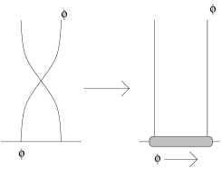
Figure 7: Counterterm with exchange of $\phi$ and $Z$.

Its value is equal to $-{1\over\epsilon}e^{i\varphi}$.

$\bullet$ one counterterm in which $\phi$ is moved one site to the left, which is the complex conjugate of the above one.

$\bullet$ $J-2$ counterterms with interactions between two $Z$ lines in which $\phi$ keeps its original position. They are due to interactions among $Z$-fields (figure 8).

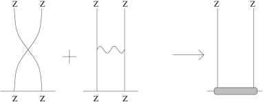
Figure 8: Counterterm for $Z$ interaction.

Each such counterterm is equal to $-{1\over\epsilon}$.

Putting together equations (17) and (18) it is not hard to see that we will cancel the divergence in the diagrams containing one insertion of ${\cal O}$ if we define the renormalized $Z_{\cal O}$ in equation (9) as:

$$Z_{\cal O}=\left(1-{\lambda\over\epsilon}(e^{i\varphi}+e^{-i\varphi}+(J-2))\right)$$ (19)

The last step is finding the wave function renormalization $Z_{3}^{\phi}$ and $Z_{3}^{Z}$. The full correction to the propagator will turn out to be useful in the two loop computation so we will write it down in detail.

3.4 One loop corrections to the propagator and the anomalous dimension.

Let us start with computing the one loop correction to the propagator of the scalar field ($\phi$ or $Z$). There are three diagrams

$${1\over p^{2}}+{\lambda\over p^{4}}\left[\int d^{4}k{(k+2p)^{2}\over k^{2}(k+p)^{2}}+8\int d^{4}k{k(k+p)\over k^{2}(k+p)^{2}}-9\int{d^{4}k\over k^{2}}\right]={1\over p^{2}}-2\lambda\left[{1\over\epsilon}+2-C\right]{1\over(p^{2})^{1+\epsilon}}$$ (20)

where the first term in parentheses comes from a gauge boson loop, the second one from a fermion loop while the third one from a scalar tadpole. Therefore the renormalization of the propagator is:

$$Z_{3}^{\phi}=Z_{3}^{Z}=1+2{\lambda\over\epsilon}$$ (21)

Combining the analogue of the equation (9) for the operator considered here (only one insertion of $\phi$) with equations (19) and (21) we find that

$$Z(\lambda,\epsilon)=Z_{\phi}^{J/2}Z_{\cal O}=1-{\lambda\over\epsilon}(e^{i\varphi}+e^{-i\varphi}-2)$$ (22)

which implies that the one loop contribution to the anomalous dimension of the operator ${\cal O}$ is

$$c_{1}(\lambda)={\lambda\over\epsilon}(e^{i\varphi}+e^{-i\varphi}-2)\,,$$ (23)

in accord with equation (12). The fact that $c_{1}$ depends on $\lambda$ only as $\lambda(e^{i\varphi}+e^{-i\varphi}-2)$ is at one loop level a consequence of supersymmetry.

We are now ready to discuss the two loop contribution to the anomalous dimension.

4 Two loops.

As discussed in section (2), the two loop contribution to anomalous dimensions has a natural expansion in terms of $e^{i\varphi}$ as

$$c_{2}=c_{2,0}+c_{2,1}(e^{i\varphi}+e^{-i\varphi})+c_{2,2}(e^{2i\varphi}+e^{-2i\varphi})$$ (24)

In the next subsection we will compute the last coefficient, $c_{2,2}$. We will continue by computing $c_{2,1}$ and finish by extracting $c_{2,0}$ from the fact that, for $\varphi=0$, the operator ${\cal O}$ is BPS and thus has vanishing anomalous dimension.

4.1 Diagrams proportional to $e^{2i\varphi}$.

As stated in section 2, there is just one diagram contributing to $c_{2,2}$. This diagram involves only interactions of scalar fields and is shown in figure 9.

Figure 9: The unique contribution to $c_{2,2}$.

The amplitude reads:

$$I_{2}(p_{1},p_{2},p_{3})=\lambda^{2}e^{2i\varphi}\int{d^{4-2\epsilon}rd^{4-2\epsilon}q\over r^{2}(r+q)^{2}(q-p_{1})^{2}(q-(p_{1}+p_{2}+p_{3}))^{2}}=$$

$$=\lambda^{2}e^{2i\varphi}{\Gamma(\epsilon)\Gamma(1-\epsilon)^{2}\over\Gamma(2-2\epsilon)}\int{d^{4-2\epsilon}q\over[q^{2}]^{\epsilon}(q-p_{1})^{2}(q-(p_{1}+p_{2}+p_{3}))^{2}}$$ (25)

To analyze the properties of this last integral, let us consider the generic expression

$$\int{d^{4-2\epsilon}q\over[q^{2}]^{\epsilon}(q-p)^{2}(q-p^{\prime})^{2}}~{}~{}.$$ (26)

This integral is logarithmically divergent, and up to

terms proportional to $\epsilon$ it is a function of $p-p^{\prime}$. Indeed,

$$\int d^{4-2\epsilon}q\left({\partial\over\partial p_{\mu}}+{\partial\over\partial p^{\prime}_{\mu}}\right){1\over[q^{2}]^{\epsilon}(q-p)^{2}(q-p^{\prime})^{2}}=-\int{d^{4-2\epsilon}q\over[q^{2}]^{\epsilon}}{\partial\over\partial q_{\mu}}{1\over(q-p)^{2}(q-p^{\prime})^{2}}=$$

$$=-\epsilon\int d^{4-2\epsilon}q{2q^{\mu}\over[q^{2}]^{1+\epsilon}(q-p)^{2}(q-p^{\prime})^{2}}$$ (27)

The integral is convergent, therefore this expression is zero up to terms of order $\epsilon$. Such precision is enough for the computation of anomalous dimensions at this order, and therefore $I(p_{1},p_{2},p_{3})$ is, for our purposes, a function of $p_{2}+p_{3}$:

$$I(p_{1},p_{2},p_{3})=\lambda^{2}e^{2i\varphi}{\Gamma(\epsilon)\Gamma(1-\epsilon)^{2}\over\Gamma(2-2\epsilon)}\int{d^{4-2\epsilon}q\over[q^{2}]^{\epsilon+1}(q-(p_{2}+p_{3}))^{2}}=$$

$$=\lambda^{2}e^{2i\varphi}{1\over[(p_{2}+p_{3})^{2}]^{2\epsilon}}{1\over\epsilon(1-2\epsilon)}{\Gamma(2\epsilon)\Gamma(1-\epsilon)^{3}\over\Gamma(2-3\epsilon)}$$ (28)

Subtracting the counterterm in figure 7 we arrive at a local divergence:

$$I_{2}(p_{1},p_{2},p_{3})-{\lambda e^{i\varphi}\over\epsilon}I_{1}(p_{2}+p_{3})=\lambda^{2}e^{2i\varphi}\left[-{1\over 2\epsilon^{2}}+{1\over 2\epsilon}+\mbox{finite}\right]~{}~{}.$$ (29)

One can easily extract from here the contribution to $c_{2,2}$. We will, however, postpone this to the end of this section when we will find the full two-loop result.

4.2 Diagrams with $e^{i\varphi}$.

The set of diagrams leading to a shift in the position of $\phi$ by one site can be naturally decomposed in three disjoint sets: diagrams with only two interacting legs, diagrams with three interacting legs and diagrams with disconnected one-loop graphs. Once the counterterms are included, the three sets of diagrams lead only to local divergences. This is the case since there are no one-loop counterterm graphs mixing any two of the three sets of diagrams.

We should take into account the contribution of the fermions. In computing the fermionic loops we will use the dimensional regularization via the dimensional reduction which was first suggested in [34]. It uses the four-dimensional algebra of gamma-matrices and four-dimensional tensor algebra, but the momenta are taken to be $(4-2\epsilon)$-dimensional. This regularization is consistent at low orders of perturbation theory as long as antisymmetric Levi-Civita tensors are not present, and manifestly preserves supersymmetry. (See the discussion in [35].)

We will begin by computing the diagrams with “two interacting legs” shown in figure 10.

Figure 10: Generic diagram with “two interacting legs”.

In this figure the dashed circle denotes the one loop corrected interaction vertex of four scalars. We will start with computing this object. In this computation we will use the following convention about the external lines. Two external lines carrying momenta $p_{1},p_{2}$ are considered amputated. The other two external lines carrying momenta $p_{3}$ and $p_{4}$ are the propagators of $\phi$ and $Z$ respectively.

For further convenience let us introduce the notation:

$$[q_{1},q_{2},q_{3},q_{4}]:=(q_{1}\cdot q_{2})(q_{3}\cdot q_{4})+(q_{1}\cdot q_{4})(q_{2}\cdot q_{3})-(q_{1}\cdot q_{3})(q_{2}\cdot q_{4})$$ (30)

The relevant 1PI diagrams are:

Figure 11: Fermion loop contribution to the 4-point scalar vertex.

$\bullet$ Figure 11 with amplitude:

$$I_{square}=4\int d^{4}k{[k,k+p_{2},k+p_{1}+p_{2},k-p_{3}]\over k^{2}(k+p_{2})^{2}(k+p_{1}+p_{2})^{2}(k-p_{3})^{2}}$$ (31)

Figure 12: Pure scalar contribution to the 4-point scalar vertex.

$\bullet$ Figure 12 with amplitude:

$$I_{fish}=-\int d^{4}k{k^{2}(k+p_{1}+p_{2})^{2}+(k-p_{3})^{2}(k+p_{2})^{2}\over k^{2}(k+p_{2})^{2}(k+p_{1}+p_{2})^{2}(k-p_{3})^{2}}$$ (32)

Figure 13: Scalar and vector contribution to the 4-point scalar vertex.

$\bullet$ Figure 13 with amplitude:

$$I_{triangle}= {1\over 2}\int d^{4}k{1\over k^{2}(k+p_{2})^{2}(k+p_{1}+p_{2})^{2}(k-p_{3})^{2}}\times$$ (34)

$$\times\left[(k+p_{2})^{2}((k+p_{3})\cdot(k+p_{3}+2p_{1}+2p_{2}))+\right.$$

$$\left.+k^{2}((k+p_{2}-p_{1})\cdot(k-p_{1}-p_{2}-2p_{3}))+\right.$$

$$\left.+(k-p_{3})^{2}((k-p_{2})\cdot(k+2p_{1}+p_{2}))+\right.$$

$$\left.+(k+p_{1}+p_{2})^{2}((k+2p_{2})\cdot(k-2p_{3}))\right]$$

Since we are interested in finding the $Z$-factor of the full graph, we will discard terms that are finite after this vertex correction is inserted into the larger diagram. In particular, using power counting, it is easy to see that we will need to keep terms proportional to $k^{4}$, $k^{3}p_{3}$ and $p_{3}^{2}$. The last two terms are divergent only after the one loop graph is inserted in the two-loop one, while the first term leads to divergences already at the one-loop level. Using these observations, the sum of all these diagrams has the following expression:

$$I_{square}+I_{fish}+I_{triangle}=$$

$$= \int d^{4}k{4k^{4}-4k^{2}(k\cdot p_{3})+p_{3}^{2}[(k\cdot p)-2(k\cdot p_{2})-(p\cdot p_{2})]+\ldots\over k^{2}(k+p_{2})^{2}(k+p_{1}+p_{2})^{2}(k-p_{3})^{2}}$$ (35)

where the dots stand for the terms which are less than quadratic in $p_{3}$ and therefore are convergent in the full graph. The integral over $k$ is divergent because of the first term in the numerator. Thus, finiteness of the vertex correction requires introduction of a counterterm equal to $-{4\over\epsilon}$.

The full diagram (figure 10) receives contributions from two one-loop counterterms. First, we have the counterterm we have just introduced which brings

$$I_{ct,\lambda}=-{4\over\epsilon}\left({1\over\epsilon}+2-C+\log{1\over p^{2}}\right)~{}~{}.$$ (36)

Furthermore, there is the contribution due to the counterterm to the one-loop interaction exchanging the positions of $\phi$ and $Z$. In the two-loop context it produces:

Figure 14: Exchange counterterm contribution to the “two interacting legs” diagrams.

$$I_{ct}={1\over 2\epsilon}\int d^{4}k{(k+p_{2})^{2}-(k-p_{2})\cdot(k+p_{2}+2p_{1})\over k^{2}(k+p_{2})^{2}(k+p)^{2}}=$$

$$={1\over\epsilon}\int d^{4}k{(k\cdot p_{2})-(k\cdot p_{1})+(p\cdot p_{2})\over k^{2}(k+p_{2})^{2}(k+p)^{2}}=$$ (37)

$$=\int d^{4}kd^{4}p_{3}{p_{3}^{2}[(k\cdot p_{2})-(k\cdot p_{1})+(p\cdot p_{2})]\over p_{3}^{2}(k-p_{3})^{2}(p_{3}+p)^{2}k^{2}(k+p_{2})^{2}(k+p)^{2}}$$ (38)

where the last equal sign holds only up to finite terms.

Putting everything together we find that

$$I_{square}+I_{fish}+I_{triangle}+I_{ct}+I_{ct,\lambda}=-{2\over\epsilon^{2}}+(finite)$$ (39)

This is not the whole contribution of diagrams with two interacting legs since we have to take into account the correction to the scalar propagator. The half of the relevant diagrams, including their counterterm, are pictured in figure 15.

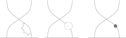
Figure 15: Scalar self-energy contribution to the “two interacting legs” diagrams

The filled circle represents the counterterm due to wave function renormalization. The other half have the self-energy and counterterm graphs inserted on the left leg. These diagrams contribute:

$$I_{se}=-4\int d^{4}k\left[\left({1\over\epsilon}+2-C\right){1\over(k^{2})^{1+\epsilon}}-{1\over\epsilon}{1\over k^{2}}\right]{1\over(k+p)^{2}}={2\over\epsilon^{2}}-{2\over\epsilon}+(finite)$$ (40)

Combining equations (39) and (40), we find that the divergent part of the diagrams with only two interacting legs is:

$$I_{2-legs}=I_{square}+I_{fish}+I_{triangle}+I_{ct}+I_{ct,\lambda}+I_{se}=-{2\over\epsilon}+\mbox{finite}$$ (41)

The remaining diagrams are those which involve three fields. We have already computed all the necessary integrals except for the graphs on Fig. 16.

Figure 16: Diagrams with vector boson exchange.

The left graph has the following amplitude:

$$I_{v}={1\over 2}\int d^{4}qd^{4}k{(q\cdot(q+2k))\over k^{2}(k+p_{1}+p_{2})^{2}(k+q)^{2}q^{4}}=$$

$$={1\over 2}\int d^{4}k{1\over k^{2}(k+p_{1}+p_{2})^{2}}\left[{\Gamma(\epsilon)\Gamma(1-\epsilon)^{2}\over\Gamma(2-2\epsilon)}{1\over[k^{2}]^{\epsilon}}-2{\Gamma(1+\epsilon)\Gamma(1-\epsilon)^{2}\over\Gamma(2-2\epsilon)}{1\over[k^{2}]^{\epsilon}}\right]+\ldots=$$

$$={1\over 2}{\Gamma(\epsilon)\Gamma(2\epsilon)\Gamma(1-\epsilon)^{3}\over\Gamma(1+\epsilon)\Gamma(2-3\epsilon)}{1\over[(p_{1}+p_{2})^{2}]^{2\epsilon}}+\ldots=$$

$$={1\over 2}\left[{1\over 2\epsilon^{2}}-{1\over 2\epsilon}+{1\over\epsilon}\left(2-C+\log{1\over(p_{1}+p_{2})^{2}}\right)\right]+\ldots$$ (42)

where dots stand for the finite part. The amplitude for the right diagram is:

$$I_{v}^{\prime}={1\over 2}\int d^{4}kd^{4}q{(q\cdot(q-2p_{2}))\over(k+p_{1}+p_{2})^{2}(k+q)^{2}(q-p_{2})^{2}q^{4}}=$$

$$={1\over 2}{\Gamma(\epsilon)\Gamma(1-\epsilon)^{2}\over\Gamma(2-2\epsilon)}\int d^{4}q{(q\cdot(q-2p_{2}))\over[(q-p_{1}-p_{2})^{2}]^{\epsilon}(q-p_{2})^{2}q^{4}}=$$

$$={1\over 2}\left[{1\over 2\epsilon^{2}}-{3\over 2\epsilon}+{1\over\epsilon}\left(2-C+\log{1\over p_{2}^{2}}\right)\right]+\ldots$$ (43)

Besides the diagrams with exchange of gauge field, there are also those which involve only scalar couplings. Their amplitude is, up to numerical factors, the same as the amplitude of the graph in figure 9. For this reason we will introduce the notation $I_{s}$ for the scalar diagram:

$$I_{s}={1\over 4\epsilon^{2}}{\Gamma(1+2\epsilon)\Gamma(1-\epsilon)^{3}\over(1-3\epsilon)(1-2\epsilon)\Gamma(1-3\epsilon)}={1\over 2}\left[{1\over 2\epsilon^{2}}+{1\over 2\epsilon}+{1\over\epsilon}(2-C)\right]$$ (44)

and express everything in terms of $I_{v}$, $I_{v^{\prime}}$ and $I_{s}$. To summarize, we have the following building blocks:

$$I_{s}={1\over 2}\left[{1\over 2\epsilon^{2}}+{1\over 2\epsilon}+{1\over\epsilon}\left(2-C+\log{1\over p^{2}}\right)\right]$$

$$I_{v}={1\over 2}\left[{1\over 2\epsilon^{2}}-{1\over 2\epsilon}+{1\over\epsilon}\left(2-C+\log{1\over(p_{1}+p_{2})^{2}}\right)\right]$$

$$I_{v^{\prime}}={1\over 2}\left[{1\over 2\epsilon^{2}}-{3\over 2\epsilon}+{1\over\epsilon}\left(2-C+\log{1\over p_{2}^{2}}\right)\right]$$

It is convenient to organize the remaining diagrams with their counterterms in four groups. Each of them leads at most to local divergencies.

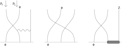
Figure 17: Group 1.

$\bullet$ Group 1 (figure 17) with amplitude

$$I_{v}+I_{s}-{1\over\epsilon}\left({1\over\epsilon}+2-C+\log{1\over(p_{1}+p_{2})^{2}}\right)=-{1\over 2\epsilon^{2}}+(finite)$$ (45)

Figure 18: Group 2.

$\bullet$ Group 2 (figure 18) with amplitude:

$$I_{v}-I_{s}=-{1\over 2\epsilon}+(finite)$$ (46)

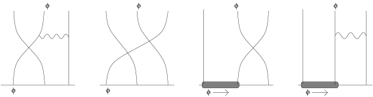
Figure 19: Group 3.

$\bullet$ Group 3 (figure 19) with amplitude:

$$I^{\prime}_{v}-I_{s}+{1\over 2\epsilon}\left({1\over\epsilon}+2-C+\log{1\over p_{2}^{2}}\right)-{1\over 2\epsilon}\left({1\over\epsilon}-C+\log{1\over p_{2}^{2}}\right)=0+(finite)$$ (47)

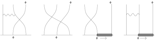
Figure 20: Group 4.

$\bullet$ Group 4 (figure 20) with amplitude:

$$I^{\prime}_{v}+I_{s}-{1\over 2\epsilon}\left({1\over\epsilon}+2-C+\log{1\over p_{1}^{2}}\right)-{1\over 2\epsilon}\left({1\over\epsilon}-C+\log{1\over p_{1}^{2}}\right)=-{1\over 2\epsilon^{2}}+{1\over 2\epsilon}+(finite)$$ (48)

Adding the contribution of the four groups we find that their amplitude is:

$$I_{3-legs}=-{1\over\epsilon^{2}}+\mbox{finite}$$ (49)

The third and last set of diagrams contains disconnected one-loop subdiagrams. The relevant ones are depicted in figure 21.

Figure 21: Diagrams containing disconnected one-loop subdiagrams.

The divergent part of their amplitude is:

$$I_{non-local}=-{1\over\epsilon^{2}}(J-3)$$ (50)

Adding up all the two loop diagrams, we find the following divergent part:

$$I_{2-loop,\;e^{i\varphi}}=I_{2-legs}+I_{3-legs}+I_{non-local}=-{1\over\epsilon^{2}}(J-2)-{2\over\epsilon}$$ (51)

from where the $Z$-factor proportional to $e^{i\varphi}$ can be extracted.

4.3 Renormalization of ${\cal O}$ at two loops.

We now turn to the renormalization of the operator ${\cal O}$ at two loops. Adding (29) and (51) we find the divergent part of the two loop diagrams with the insertion of ${\cal O}$:

$$\lambda^{2}\left[e^{2i\varphi}\left(-{1\over 2\epsilon^{2}}+{1\over 2\epsilon}\right)+e^{i\varphi}\left(-{J-2\over\epsilon^{2}}-{2\over\epsilon}\right)+{A_{2,2}\over\epsilon^{2}}+{A_{2,1}\over\epsilon}+\mbox{finite}\right]$$ (52)

Here ${A_{2,2}\over\epsilon^{2}}+{A_{2,1}\over\epsilon}$ is the contribution of the diagrams without the exchange of $Z$ and $\phi$ which we have not computed explicitly.

From here and equation (19) we find that $Z_{\cal O}$ in equation (9) has the following two-loop expression:

$$Z_{{\cal O},\;2-loop}=1-{\lambda\over\epsilon}(e^{i\varphi}+e^{-i\varphi}+(J-2))+$$

$$+{\lambda^{2}\over\epsilon^{2}}\left({1\over 2}(e^{2i\varphi}+e^{-2i\varphi})+(J-2)(e^{i\varphi}+e^{-i\varphi})-A_{2,2}\right)+$$ (53)

$$+{\lambda^{2}\over\epsilon}\left(-{1\over 2}(e^{2i\varphi}+e^{-2i\varphi})+2(e^{i\varphi}+e^{-i\varphi})-A_{2,1}\right)$$ (54)

We are left with the task of determining the various unknown coefficients in the above equation. One way of determining them is doing the explicit computation and finding the contribution of diagrams with no exchange of $Z$ and $\phi$. This is a rather tedious exercise, since the number of diagrams is substantially larger than those considered by now. The easier way is to notice that, for $\varphi=0$ our operator is BPS and therefore has vanishing anomalous dimension. This means that the $Z$ factor for $\varphi=0$ cancel against the renormalization of external lines. In other words

$$\left.Z_{\phi}^{-J/2}Z_{\cal O}\right|_{\varphi=0}=1~{}~{}.$$ (55)

Combining this with equation (4.3) we get

$$Z_{\phi}^{-J/2}Z_{\cal O}=\exp\left\{{1\over\epsilon}\left[-\lambda(e^{i\varphi}+e^{-i\varphi}-2)-{\lambda^{2}\over 2}(e^{i\varphi}+e^{-i\varphi}-2)^{2}+\ldots\right]\right\}$$ (56)

which exactly agrees with equation (12).

To summarize this section, we have verified at the two loop level that the renormalization of ${\cal O}$ depends on the coupling constant $\lambda$ only in the combination $\lambda(e^{i\varphi}+e^{-i\varphi}-2)$.

5 Higher orders

In the previous section we have computed the two-loop contribution to the anomalous dimension of operators dual to stringy excitations and found that the conjecture put forward in section 2 holds at this order. The contribution of the many diagrams leading to this result is quite entangled and a pattern of cancellations that can be generalized to all loop order does not seem to emerge. However, assuming that the conjecture (12) holds, we can actually derive the anomalous dimension to all orders in perturbation theory. The idea is that, given this assumption, there is exactly one relevant diagram per loop order. In this section we will compute all these diagrams. We will sum these graphs and argue that the anomalous dimension is indeed given by (2).

5.1 Subset of diagrams.

By briefly studying the diagrams at an arbitrary loop order $L$, it is not difficult to see that there is only one that requires a counterterm proportional to $e^{iL\varphi}$. This diagram involves only scalar field couplings and at each vertex $\phi$ and $Z$ switch places. A generic graph of this type is shown in figure 22. Under the assumption stated above, this diagram gives the only contribution to the anomalous dimension at L loops.

We will now compute the contribution of figure 22. In principle one should put arbitrary momenta on external lines.

Figure 22: The $j$-loop diagram contribution to $c_{j,j}$, $j=3$ is shown.

However, as long as infrared divergences are not encountered, we can make further simplifying assumptions, in particular, we can set some momenta to zero since this does not change the divergent part. In figure 22 we put different momenta on the $Z$ legs and on the $\phi$ legs. Using the argument above we will compute this diagram in the limit $p_{Z}\to 0$. The corresponding Feynman integral is:

$$I_{n}(p_{\phi})=\int{d^{4-2\epsilon}r_{1}\over r_{1}^{2}(r_{1}-r_{2})^{2}}\int{d^{4-2\epsilon}r_{2}\over r_{2}^{2}(r_{2}-r_{3})^{2}}\cdots\int{d^{4-2\epsilon}r_{n}\over r_{n}^{2}(r_{n}-p_{\phi})^{2}}$$ (57)

Probably the easiest way of computing this integral is to set up a recurrence relation based on the following identity:

$$\int d^{4}q{1\over[q^{2}]^{1+n\epsilon}(q-p)^{2}}={\Gamma(1-\epsilon)\Gamma((n+1)\epsilon)\Gamma(1-(n+1)\epsilon)\over\Gamma(1+n\epsilon)\Gamma(2-(n+2)\epsilon)}{1\over[p^{2}]^{(n+1)\epsilon}}$$ (58)

Then, solving the recurrence, we find that the integral (57) is given by:

$$I_{n}(p_{\phi})={1\over(n-1)!}{\Gamma(n\epsilon)\over\epsilon^{n-1}}{\Gamma(1-\epsilon)^{n+1}\over\Gamma(2-(n+1)\epsilon)}\times{1\over(1-2\epsilon)\cdots(1-n\epsilon)}\times{1\over[p_{\phi}^{2}]^{n\epsilon}}$$ (59)

We now have all ingredients that will lead to the proof that equation (2) holds to all orders in perturbation theory

5.2 The renormalized sum of the diagrams.

Assuming that the coupling constant enters the formula for the anomalous dimension in the combination ${\hat{\lambda}}=\lambda(e^{i\varphi}+e^{-i\varphi}-2)$ as stated in equation (12), the $Z$-factor for an operator ${\cal O}$ of anomalous dimension $c({\hat{\lambda}})$:

$$Z=\exp\left[{1\over\epsilon}\int\limits_{0}^{1}{dt\over 2t}\left(c(t{\hat{\lambda}})-1\right)\right]$$ (60)

Showing that $c-1$ is indeed its anomalous dimension amounts to showing that the product between $Z$ and the sum of regularized Feynman integrals corresponding to diagrams with one insertion of some operator ${\cal O}$ is finite. Under our assumption about the dependence on $\lambda$ the sum of regularized Feynman integrals is:

$$I(p)=1+\sum\limits_{n=1}^{\infty}{1\over n!}{{\hat{\lambda}}^{n}\over\epsilon^{n}}{\Gamma(1+n\epsilon)\Gamma(1-\epsilon)^{n+1}\over\Gamma(2-(n+1)\epsilon)\prod\limits_{k=2}^{n}(1-k\epsilon)}{1\over[p_{\phi}^{2}]^{n\epsilon}}$$ (61)

We want to show that

$$\sqrt{1-4\lambda(e^{i\varphi}+e^{-i\varphi}-2)}-1$$ (62)

is the anomalous dimension of ${\cal O}$. This is equivalent to the statement that

$$I^{ren}(p)=\exp\left[{1\over\epsilon}\int\limits_{0}^{1}{dt\over 2t}(\sqrt{1-4t{\hat{\lambda}}}-1)\right]I(p)$$ (63)

is finite as $\epsilon\rightarrow 0$. One can indeed verify order by order in $\hat{\lambda}$ that (63) is finite. There is also a general argument which we now describe.

Notice that the integral in the exponent can be explicitly computed and it gives

$$\exp\left[{1\over\epsilon}\int_{0}^{1}{dt\over 2t}(\sqrt{1-4{\hat{\lambda}}t}-1)\right]=\exp\left\{{1\over\epsilon}\left[\sqrt{1-4{\hat{\lambda}}}-1+\log{2\over 1+\sqrt{1-4{\hat{\lambda}}}}\right]\right\}$$ (64)

This has to be canceled by a similar contribution coming from the sum of Feynman diagrams. To find the leading exponential behaviour of $I(p)$ we represent the sum as an integral and use the saddle point approximation:

$$\begin{array}[]{l}I(p)\sim\int\limits^{\infty}{1\over\epsilon}dx{\Gamma(1+x)\over\Gamma(2-x)}{\left({{\hat{\lambda}}\over\epsilon}\right)^{x\over\epsilon}\over(x/\epsilon)!}\exp\left[-{1\over\epsilon}\left((1-x)\log(1-x)+x)\right)\right]=\\[5.0pt] ={1\over\epsilon}\int\limits^{\infty}dx\sqrt{\epsilon\over x}f(x)\exp\left[{1\over\epsilon}\left(x(\log({\hat{\lambda}})-\log x)+2x+(1-x)\log(1-x)\right)\right]\end{array}$$ (65)

Here we have defined $x=n\epsilon$, and $f(x)$ is finite at $\epsilon\to 0$. The equation for the saddle point is then:

$$\log x_{0}(1-x_{0})=\log{\hat{\lambda}}$$ (66)

This gives $x_{0}={1-\sqrt{1-4{\hat{\lambda}}}\over 2}$. The series then is approximated by the saddle point:

$$I(p)\sim\left[{1+\sqrt{1-4{\hat{\lambda}}}\over 2}e^{1-\sqrt{1-4{\hat{\lambda}}}}\right]^{1/\epsilon}~{}~{}.$$ (67)

which is exactly the inverse of (64)! The pre-exponential factor correcting the saddle point approximation is a series in $\epsilon$, and it is finite at $\epsilon\to 0$. This proves that (63) is finite at $\epsilon=0$.

6 Conclusions.

The usual ’t Hooft perturbation theory for large $N$ field theory is an expansion in the small parameter $\lambda=g^{2}N$. Our results indicate that there are amplitudes for which the actual small parameter is not $\lambda$ but rather $\lambda\sinh^{2}\left({\varphi\over 2}\right)$. In these amplitudes, we can consider the regime when $\lambda$ is large and $\varphi$ is small, so that $\lambda\varphi^{2}\ll 1$. In this regime, the perturbative expansion is still valid even though the ’t Hooft parameter is large. On the other hand, a large ’tHooft parameter implies that the calculation can be done in the dual picture, namely string theory in a plane wave background. This means that the perturbative computation in the field theory can be compared with the perturbative computation on the string worldsheet.

We have partialy summed the perturbation series and found that the result for the anomalous dimension is indeed equal to the mass of the string excitation. This is true order by order in the Yang-Mills perturbation theory, presumably up to order roughly equal to $J$ (the R charge of the operator). At that order, $\simeq J$, we should include diagrams involving the collision of two $\phi$’s. It is possible that in these diagrams, the assumption that $\lambda$ enters in the combination $\lambda\sinh^{2}\left({\varphi\over 2}\right)$ breaks down and therefore one cannot rely on perturbation theory.

Given this success of the BMN proposal it would be very interesting to extend the perturbative calculations of the anomalous dimensions of these operators, in the large $N$ and $J$ limit, to include non-planar corrections of order $g^{2}$., These should correspond on the string side to string loop corrections to the masses of string excitations. In this way one could “derive”the interacting string theory in a plane wave background from gauge theory.

7 Acknowledgements.

We want to thank Tibor Kucs for discussions about two loop momentum integrals. The work of A.M. and D.G. was supported in part by the National Science Foundation under Grant No. PHY99-07949. The work of A.M. was partly supported by the RFBR Grant No. 00-02-116477 and in part by the Russian Grant for the support of the scientific schools No. 00-15-96557. The work of RR was supported in part by DOE under Grant No. 91ER40618(3N) and in part by the National Science Foundation under Grant No. PHY00-9809(6T).

References

- [1] J.M. Maldacena, “The Large N Limit of Superconformal Field Theories and Supergravity”, Adv.Theor.Math.Phys. 2 (1998) 231-252; Int.J.Theor.Phys. 38 (1999) 1113-1133; hep-th/9711200.
- [2] S.S. Gubser, I.R. Klebanov, A.M. Polyakov, “Gauge Theory Correlators from Non-Critical String Theory”, Phys.Lett. B428 (1998) 105-114, hep-th/9802109.
- [3] E. Witten, “Anti De Sitter Space And Holography”, Adv.Theor.Math.Phys. 2 (1998) 253-291, hep-th/9802150.
- [4] D. Berenstein, J. Maldacena, H. Nastase, “Strings in flat space and pp waves from Super Yang Mills”, hep-th/0202021.
- [5] R.R. Metsaev, ”Type IIB Green-Schwarz superstring in plane wave Ramond-Ramond background”, Nucl.Phys. B625 (2002) 70-96, hep-th/0112044.
- [6] J.G. Russo, A.A. Tseytlin, ”On Solvable Models of Type 2B Superstring in NS-NS and R-R plane Wave Backgrounds”, JHEP 0204:021,2002 hep-th/0202179
- [7] Chong-Sun Chu, Pei-Ming Ho, ”Noncommutative D Brane and Open String in PP Wave Background with B-field”, hep-th/0203186
- [8] S. Frolov, A.A. Tseytlin, ”Semiclassical Quantization of Rotating Superstring in ”, hep-th/0204226
- [9] A. Dabholkar, S. Parvizi, ”DP-Branes in PP Wave Background”, hep-th/0203231
- [10] E. Kiritsis, B. Pioline, ”Strings in Homogeneous Gravitational Waves and Null Holography”, hep-th/0204004
- [11] N. Itzhaki, I.R. Klebanov, S. Mukhi, ”PP Wave Limit and Enhanced Supersymmetry in Gauge Theories”, JHEP 0203:048,2002 hep-th/0202153
- [12] L.A. Pando Zayas, J. Sonnenschein ”On Penrose Limits and Gauge Theories”, hep-th/0202186
- [13] J. Gomis, H. Ooguri, ”Penrose Limit of Gauge Theories”, hep-th/0202157
- [14] M. Alishahiha, M.M. Sheikh-Jabbari, ”The PP Wave Limits of Orbifolded AdS(5) X S**5”, hep-th/0203018
- [15] Nak-woo Kim, A. Pankiewicz, Soo-Jong Rey, S. Theisen, ”Superstring on PP Wave Orbifold from Large N Quiver Gauge Theory”, hep-th/0203080
- [16] T. Takayanagi, S. Terashima, ”Strings on Orbifolded PP Waves”, hep-th/0203093
- [17] E. Floratos, A. Kehagias, ”Penrose Limits of Orbifolds and Orientifold”, hep-th/0203134
- [18] D. Berenstein, E. Gava, J.M. Maldacena, K.S. Narain, H. Nastase, ”Open Strings on Plane Waves and their Yang-Mills Duals”, hep-th/0203249
- [19] J. Michelson, ”Twisted Toroidal Compactification of PP Waves”, hep-th/0203140
- [20] Peter Lee, Jong-won Park, ”Open Strings in PP Wave Background from Defect Conformal Field Theory”, hep-th/0203257
- [21] Hong Lu, J.F. Vazquez-Poritz, ”Penrose Limits of Nonstandard Brane Intersections”, hep-th/0204001
- [22] U. Gursoy, C. Nunez, M. Schvellinger, ”RG Flows from SPIN(7), CY 4 fold and HK Manifolds to AdS, Penrose Limits and PP Waves”, hep-th/0203124
- [23] R. Gueven, ”Randall-Sundrum Zero Mode as a Penrose Limit”, hep-th/0203153
- [24] Yosuke Imamura, ”Large Angular Momentum Closed Strings Colliding with D-Branes”, hep-th/0204200
- [25] M. Spradlin, A. Volovich, ”Superstring Interactions in a PP Wave Background”, hep-th/0204146
- [26] C. Kristjansen, J. Plefka, G.W. Semenoff and M. Staudacher, “A New Double-Scaling Limit of N=4 Super Yang-Mills Theory and PP-Wave Strings”, hep-th/0205033.
- [27] S.R. Das, C. Gomez, Soo-Jong Rey, ”Penrose Limit, Spontaneous Symmetry Breaking and Holography in PP Wave Background”, hep-th/0203164
- [28] R.G. Leigh, K. Okuyama, M. Rozali, ”PP Waves and Holography”, hep-th/0204026
- [29] J.K. Erickson, G.W. Semenoff, K. Zarembo, “Wilson loops in N=4 supersymmetric Yang-Mills theory,” Nucl. Phys. B 582(2000) 155, hep-th/0003055; Nadav Drukker, David J. Gross, “An Exact Prediction of N=4 SUSYM Theory for String Theory”, J.Math.Phys. 42 (2001) 2896-2914, hep-th/0010274; J. Plefka and M. Staudacher, “ Two loops to two loops in N=4 supersymmetric Yang-Mills theory,” JHEP 0109 (2001) 031, hep-th/0108182; G. Arutyunov, J. Plefka and M. Staudacher, “Limiting geometries of two circular Maldacena-Wilson loop operators,” JHEP 0112, 014 (2001), hep-th/0111290
- [30] E. D’Hoker, D.Z. Freedman, W. Skiba, “Field theory tests for correlators in the AdS/CFT correspondence”, Phys.Rev. D59, 045008 (1999), hep-th/9807098.
- [31] S. Penati, A. Santambrogio, D. Zanon, “Two-Point Functions of Chiral Operators in SYM at order ”, JHEP9912 (1999) 006, hep-th/9910197; “More on correlators and contact terms in SYM at order ”, Nucl. Phys. B593 (2001) 651-670, hep-th/0005223.
- [32] F. Gonzalez-Rey, B. Kulik, I.Y. Park, “Non-renormalization of two and three Point Correlators of N=4 SYM in N=1 Superspace”, Phys.Lett. B455 (1999) 164-170, hep-th/9903094.
- [33] S. Penati, A. Santambrogio, “Superspace Approach to Anomalous Dimensions in SYM”, Nucl Phys. B614 (2001) 367-387.
- [34] W. Siegel, “Supersymmetric Dimensional Regularization via Dimensional Reduction”, Phys.Lett. B84:193, 1979; “Inconsistency of Supersymmetric Dimensional Regularization”, Phys.Lett. B94:37,1980.
- [35] L.V. Avdeev, A.A. Vladimirov, “Dimensional Regularization and Supersymmetry”, Nucl.Phys.B219:262,1983.