hep-th/0205064

PUPT-2038

String Tensions and Three Dimensional
Confining Gauge Theories

Christopher P. Herzog
Joseph Henry Laboratories,

Princeton University,

Princeton, New Jersey 08544, USA

cpherzog@princeton.edu

Abstract

In the context of gauge/gravity duality, we try to understand better the proposed duality between the fractional D2-brane supergravity solutions of (Nucl. Phys. B 606 (2001) 18, hep-th/0101096) and a confining $2+1$ dimensional gauge theory. Based on the similarities between this fractional D2-brane solution and D3-brane supergravity solutions with more firmly established gauge theory duals, we conjecture that a confining $q$-string in the $2+1$ dimensional gauge theory is dual to a wrapped D4-brane. In particular, the D4-brane looks like a string in the gauge theory directions but wraps a $\mathbf{S}^{3}\subset\mathbf{S}^{4}$ in the transverse geometry. For one of the supergravity solutions, we find a near quadratic scaling law for the tension: $T\sim q\,(N-q)$. Based on the tension, we conjecture that the gauge theory dual is $SU(N)$ far in the infrared. We also conjecture that a quadratic or near quadratic scaling is a generic feature of confining $2+1$ dimensional $SU(N)$ gauge theories.

May 2002

1 Introduction

The original AdS/CFT correspondence [1, 2, 3] has taught string theorists much about the relationships between $3+1$ dimensional gauge theories and string theory in curved space-time. The present work is motivated by the hope that this conjectured correspondence generalizes to gauge theories in other dimensions.

A duality between a certain ${\mathcal{N}}=1$ supersymmetry preserving, type IIA supergravity solution and a $2+1$ dimensional confining gauge theory was proposed by Cvetič, Gibbons, Lü, and Pope (CGLP) in [4]. The duality was motivated by the striking resemblance between this supergravity solution and the Klebanov-Strassler (KS) solution [5], which in the infrared is the well established dual of a confining $SU(N)$ gauge theory is $3+1$ dimensions. Despite the striking resemblance of the two supergravity solutions, the $2+1$ dimensional gauge theory dual of the CGLP solution has remained mysterious.

To give the reader some context, recall that the KS solution grew out of an attempt to produce a more realistic AdS/CFT correspondence. The original AdS/CFT correspondence, motivated by placing a stack of $N$ D3-branes in flat, ten dimensional space, relates ${\mathcal{N}}=4$ supersymmetric $SU(N)$ gauge theory to type IIB string theory in an $AdS_{5}\times S^{5}$ background. To reduce the amount of supersymmetry to ${\mathcal{N}}=1$, the authors of [6] placed the D3-branes at the tip of the conifold, a non-compact Calabi-Yau three-fold, producing an $SU(N)\times SU(N)$. Later, to break the conformal symmetry, the authors of [7, 8], introduced $M$ fractional D3-branes, i.e. D5-branes wrapped on vanishingly small two-cycles at the tip of the conifold, changing the gauge group to $SU(N+M)\times SU(N)$. The original supergravity solution [8] describing these fractional branes, also called the Klebanov-Tseytlin or KT solution, had a singularity. The KS solution eliminates the singularity by deforming the conifold. On the gauge theory side, the deformation was related to chiral symmetry breaking and confinement.

In an attempt to generalize some of this work to gauge theories in other dimensions, [9, 4, 10] produced analogs of the KT and KS supergravity solutions for fractional D$p$-branes, $p\neq 3$, positioned at conical singularities. Although most of these supergravity solutions are well behaved in the UV and some are well-behaved everywhere, the gauge theory duals often remain mysterious. In this paper, we focus on just one of these supergravity solutions, the fractional D2-brane solution presented in [4]. Some recent progress toward understanding the ultraviolet region of the gauge theory was made by [11]. The present work is in large part motivated by the need to understand better the infrared, confining region of this gauge theory.

In particular, we will use confining strings to probe the infrared of this $2+1$ dimensional gauge theory. In an $SU(N)$ theory, confining strings can be thought of as flux tubes joining $q$ probe quarks with $q$ probe anti-quarks, where $q$ ranges from 1 to $N-1$. For $q=N$, the quarks can combine into a baryon, and the string becomes tensionless. Moreover, there is a symmetry under $q\rightarrow N-q$ which corresponds to replacing quarks with anti-quarks. Finally, one expects these confining strings to be stable with respect to decay into strings with fewer numbers of quarks:

$$T_{q+q^{\prime}}<T_{q}+T_{q^{\prime}}\ .$$ (1)

In other words, the tension should be a convex function with respect to $q$.

For the other simple Lie groups, there are typically far fewer types of confining strings because because the gluons are more effective at screening charge. The allowed charges are described by the center of the Lie group. For $SU(N)$, the center is $\mathbb{Z}_{N}$ while for the other simple Lie groups, the center is much smaller, for example, $\mathbb{Z}_{2}$, $\mathbb{Z}_{2}\times\mathbb{Z}_{2}$, or $\mathbb{Z}_{4}$. It is important to keep in mind that we don’t know for sure what the gauge group of this $2+1$ dimensional theory is.

We propose that the confining strings are dual to certain wrapped D4-branes in the CGLP supergravity solution. The proposal is motivated by the fact that these D4-branes are the analog of certain wrapped D3-branes considered by [12] for the KS solution. The authors of [12] argued that these D3-branes were the confining strings of the ${\mathcal{N}}=1$ $SU(N)$ confining gauge theory dual.

The tension of the confining strings or equivalently of these wrapped D4-branes allows us to make a conjecture about the confining $2+1$ dimensional gauge theory. Treating these wrapped D4-branes as a small perturbation on the background geometry, we calculate the tension of the confining strings using the DBI action.

In order to understand the conjecture, one should understand that there are actually two, not just one, CGLP supergravity solutions under discussion, and that there are as a result possibly two distinct $2+1$ dimensional confining gauge theories. Both CGLP solutions are warped compactifications of three dimensional Minkowski space and a noncompact, asymptotically conical, $G_{2}$ manifold. The warp factor depends on the radius associated with the asymptotically conical limit. One $G_{2}$ manifold, $\mathbf{Y}_{S}$, is a $\mathbb{R}^{3}$ fibration over $\mathbf{S}^{4}$ while the other, $\mathbf{Y}_{P}$, is a $\mathbb{R}^{3}$ fibration over $\mathbb{CP}^{2}$ [13]. Both solutions are stabilized by $N$ units of $F_{4}$ flux that thread four cycles inside the $G_{2}$ manifolds. This $F_{4}$ flux should correspond to $N$ “fractional” D2-branes, i.e. D4-branes wrapped on vanishing two cyles inside the $G_{2}$ manifold.

The conjecture is that the confining gauge theory dual to the supergravity solution involving $\mathbf{Y}_{S}$ has gauge group $SU(N)$ far in the infrared. The manifold $\mathbf{Y}_{S}$ leads to a formula for the string tensions that is nearly quadratic:

$$T\sim q\,(N-q)\ .$$ (2)

By nearly, we mean that the non-quadratic corrections are small compared to the $q(N-q)$ term. The facts that $T$ is symmetric under $q\rightarrow N-q$, that $T$ vanishes at $q=N$, and that $T$ is convex strongly suggest that the gauge group is $SU(N)$.

The quadratic or Casimir scaling of the string tensions is interesting because it may hold true for a much larger class of three dimensional confining theories than the one considered here. Such a quadratic or Casimir scaling hypothesis was put forward many years ago by Ambjorn, Olesen, and Peterson [14]. Lucini and Teper [15] have also found evidence for such a quadratic, or near quadratic, scaling for $SU(4)$ and $SU(6)$ gauge theories in $2+1$ dimensions on the lattice.

Another line of evidence for the universality of such a formula comes from experience with confining strings in $3+1$ dimensional $SU(N)$ gauge theories. Much evidence has accumulated that these string tensions obey a sine law.

$$T\sim\sin\left(\frac{\pi q}{N}\right)\ .$$ (3)

Douglas and Shenker [17] using softly broken ${\mathcal{N}}=2$ gauge theory and Hanany, Strassler, and Zaffaroni [18] in the MQCD approach to ${\mathcal{N}}=1$ supersymmetric gauge theory find this sine law. The wrapped D3-branes in the KS geometry [12] obey nearly such a sine law. In the context of nonsupersymmetric gauge theory, the authors of [15, 19] using a Monte Carlo simulation on a lattic have found numerical evidence for such a scaling for non-supersymmetric $SU(4)$, $SU(5)$, and $SU(6)$ gauge theories. The list goes on (see for example [20] or [21]).

Our second conjecture is then that this quadratic or near quadratic scaling is a common feature of $2+1$ dimensional confining $SU(N)$ gauge theories.

The situation is less clear for $\mathbf{Y}_{P}$. The maximum number of confining strings appears to be non-integer and less than $N$. Additionally, the tension formula does not vanish at $q_{max}$ and does not have a $\mathbb{Z}_{2}$ symmetry. Perhaps some of the confining strings we have found are unstable.

We begin by reviewing the CGLP supergravity solutions in greater detail. In the appendix, there is an independent derivation of these solutions from a first order system of differential equations. The first order system is derived from a one dimensional effective action. In section 3, we present the details of the confining string calculations.

2 The CGLP Supergravity Solutions

In order to extract meaningful results from the confining string calculation in section 3, we need to normalize carefully the two CGLP supergravity solutions [4]. In the same way that the normalizations found in [23] laid the groundwork for the confining string calculations in [12], this section lays the groundwork for the tensions we calculate in the next. So the reader can understand where the normalizations come from, in the following section we have reproduced some of what can be found in [4] or [13].

The two CGLP supergravity solutions under investigation are closely related to the type IIA supergravity solution corresponding to a stack of D2-branes placed in flat ten dimensional space. The CGLP solutions are built out of a warped compactification of $2+1$ dimensional Minkowski space and an asymptotically conical $G_{2}$ manifold $\mathbf{Y}$. Hence the metric is

$$ds_{10}^{2}=H(r)^{-5/8}dx^{\mu}dx^{\nu}\eta_{\mu\nu}+H(r)^{3/8}ds_{\mathbf{Y}}^{2}\ .$$ (4)

The variable $r$ is the radius of the asymptotically conical region of $\mathbf{Y}$.

The metric of $\mathbf{Y}$ can be written down for arbitrary $r$. In both cases, $\mathbf{Y}$ is an $\mathbb{R}^{3}$ bundle over a four dimensional Einstein manifold $M_{4}$.

$$ds_{\mathbf{Y}}^{2}=\ell^{2}\left[h(r)^{2}dr^{2}+a(r)^{2}(D\mu^{i})^{2}+b(r)^{2}ds_{M_{4}}^{2}\right]\ .$$ (5)

The coordinates on $\mathbf{Y}$ are all dimensionless, so the length scale $\ell$ has been introduced to give the metric the right scaling. In one case, $\mathbf{Y}=\mathbf{Y}_{S}$ and $M_{4}=\mathbf{S}^{4}$, and in the other, $\mathbf{Y}=\mathbf{Y}_{P}$ and $M_{4}=\mathbb{CP}^{2}$. The Einstein condition on $M_{4}$ is such that $R_{ab}=3g_{ab}$. Now, the $\mu^{i}$ are coordinates on the $\mathbb{R}^{3}$ subject to $\mu^{i}\mu^{i}=1$. The fibration is written in terms of $SU(2)$ Yang-Mills instanton potentials $A^{i}$ where

$$D\mu^{i}=d\mu^{i}+\epsilon_{ijk}A^{j}\mu^{k}\ .$$ (6)

The field strengths $J^{i}\equiv dA^{i}+\frac{1}{2}\epsilon_{ijk}A^{j}\wedge A^{k}$ satisfy the algebra of the unit quaternions $J_{\alpha\gamma}^{i}J_{\gamma\beta}^{j}=-\delta_{ij}\delta_{\alpha\beta}+\epsilon_{ijk}J_{\alpha\beta}^{k}$.

The metric (5) is Ricci-flat and has $G_{2}$ holonomy when the functions $h$, $a$, and $b$ satisfy

$$h^{2}=\left(1-\frac{1}{r^{4}}\right)^{-1}\;,\;\;\;a^{2}=\frac{1}{4}r^{2}\left(1-\frac{1}{r^{4}}\right)\;,\;\;\;b^{2}=\frac{1}{2}r^{2}\ .$$ (7)

The variable $r$ runs from one to infinity. Performing the rescaling $R=r\ell$, one sees that this parameter $\ell$ is very similar to the deformation parameter $\epsilon$ of the deformed conifold [5]. At the tip $r=1$ of this deformed cone, the $\mathbb{R}^{3}$ directions vanish while the $M_{4}$ remains finite:

$$ds_{\mathbf{Y}}^{2}\rightarrow\frac{\ell^{2}}{2}ds^{2}_{M_{4}}\ .$$ (8)

In the other limit $r\rightarrow\infty$, the metric approaches that of a cone over a squashed Einstein manifold. The metric separates into two pieces:

$$ds_{\mathbf{Y}}^{2}=\ell^{2}\left[dr^{2}+r^{2}ds_{\mathbf{X}}^{2}\right]$$ (9)

where $\mathbf{X}$ is a six dimensional “squashed” Einstein manifold satisfying $R_{ab}=5g_{ab}$. In particular, this squashed metric is nearly Kähler, a technical condition with some unsettling consequences (see, for example [24]). For example, the first Chern class vanishes on nearly Kähler spaces even though the Ricci curvature does not always. For the case $\mathbf{Y}_{S}$, the Einstein manifold is a squashed $\mathbb{CP}^{3}$ while for $\mathbf{Y}_{P}$, the Einstein manifold is the nearly Kähler flag manifold $SU(3)/T^{2}$, where $T^{2}$ is a maximal torus in $SU(3)$.

There are also fluxes that stabilize the metric. The four form RR flux $F_{4}$ has two pieces, one corresponding to the electric flux of the ordinary D2-branes aligned in the Minkowski space-time directions, the other corresponding to magnetic flux from the “fractional” D2-branes. These fractional D2-branes are D4-branes wrapped on vanishing 2-cycles inside $\mathbf{Y}$. As a result, they source a flux through a transverse 4-cycle inside $\mathbf{Y}$:

$$g_{s}F_{4}=d^{3}x\wedge dH^{-1}+mG_{4}\ .$$ (10)

Just as in the standard D2-brane solution where $m=0$, the dilaton is nonzero, $e^{\phi}=g_{s}H^{1/4}$.

Finally, to satisfy the supergravity equations of motion, a nonzero $m$ forces one to turn on the NSNS three form flux

$$H_{3}=mG_{3}\ ,$$ (11)

where $G_{3}$ is a harmonic 3-form inside $\mathbf{Y}$ and $G_{4}=\star G_{3}$ with $\star$ the Hodge dual with respect to $ds_{\mathbf{Y}}^{2}$. The trace of Einstein’s equations enforces the condition on the warp factor

$$\square H=-\frac{1}{6}m^{2}|G_{3}|^{2}\$$ (12)

where $\square$ is the Laplacian with respect to $ds_{\mathbf{Y}}^{2}$ and the magnitude $|\cdots|^{2}$ is also taken with respect to $ds_{\mathbf{Y}}^{2}$.

The harmonic 3-form $G_{3}$ is

$$\ell G_{3}=f_{1}(r)\,dr\wedge X_{2}+f_{2}(r)\,dr\wedge J_{2}+f_{3}(r)\,X_{3}$$ (13)

where

$$X_{2}\equiv\frac{1}{2}\epsilon_{ijk}\mu^{i}D\mu^{j}\wedge D\mu^{k}\;,\;\;\;J_{2}\equiv\mu^{i}J^{i}\;,\;\;\;X_{3}\equiv D\mu^{i}\wedge J^{i}\ .$$ (14)

The forms obey

$$dX_{2}=X_{3}\;,\;\;\;dJ_{2}=X_{3}\;,\;\;\;dX_{3}=0\ .$$ (15)

Using these relations and the fact that $f_{3}^{\prime}=f_{1}+f_{2}$, one can choose a gauge such that

$$\ell B_{2}=m\left(\int_{1}^{r}f_{1}(u)du\right)X_{2}+m\left(\int_{1}^{r}f_{2}(u)du\right)J_{2}$$ (16)

and $dB_{2}=H_{3}$. Note that at $r=1$, $B_{2}$ vanishes.

The dual four form $G_{4}$ is

$$G_{4}=f_{3}h\,\epsilon_{ijk}\mu^{i}dr\wedge D\mu^{j}\wedge J^{k}+\frac{f_{2}a^{2}}{h}X_{2}\wedge J_{2}+\frac{f_{1}b^{4}}{2ha^{2}}J_{2}\wedge J_{2}\ .$$ (17)

One then solves for the $f_{i}$ using the fact that $dG_{4}=0$ and that $G_{4}$ should be responsible for a constant flux from the the fractional D2-branes. The result is

$$f_{1}=ha^{2}u_{1}\;,\;\;\;f_{2}=hb^{2}u_{2}\;,\;\;\;f_{3}=ab^{2}u_{3}\ ,$$ (18)

where

$$u_{1} = \frac{1}{r^{4}}+\frac{P(r)}{r^{5}(r^{4}-1)^{1/2}}\ ,$$

$$u_{2} = -\frac{1}{2(r^{4}-1)}+\frac{P(r)}{r(r^{4}-1)^{3/2}}\ ,$$ (19)

$$u_{3} = \frac{1}{4r^{4}(r^{4}-1)}-\frac{(3r^{4}-1)P(r)}{4r^{5}(r^{4}-1)^{3/2}}\ ,$$

and where

$$P(r)=\int_{1}^{r}\frac{d\rho}{\sqrt{\rho^{4}-1}}\ .$$ (21)

We will now attempt to quantize $G_{4}$ flux by looking at the limit $r\rightarrow 1$. In this limit, the $u_{i}$ all become constant:

$$u_{1}\rightarrow\frac{3}{2}\;,\;\;\;u_{2}\rightarrow-\frac{1}{4}\;,\;\;\;u_{3}\rightarrow-\frac{1}{4}\;.$$ (22)

However, the choice of radial variable introduces a coordinate singularity to the metric because

$$h^{2}dr^{2}\rightarrow\frac{dr^{2}}{4(r-1)}\ .$$ (23)

It would be best to introduce a new radial variable $\tau$ such that $d\tau\sim dr/\sqrt{r-1}$. However, we will just pretend that $h\,dr$ is well behaved in the limit $r=1$. Putting the pieces together, in the limit $r\to 1$,

$$G_{4}\rightarrow\frac{3}{8}\mathrm{vol}(M_{4})\ ,$$ (24)

where we have used the fact that $J_{2}\wedge J_{2}=2\mathrm{vol}(M_{4})$.

From the Dirac quantization condition, we know what the integral of $F_{4}$ over the $M_{4}$ at the tip of the cone should be

$$\int_{M_{4}}F_{4}=8\pi^{3}\alpha^{\prime 3/2}N$$ (25)

where $N$ is the number of fractional D2-branes. As the volume of a unit $\mathbf{S}^{4}$ is $8\pi^{2}/3$ and the volume of our $\mathbb{CP}^{2}$ is $2\pi^{2}$, one finds that for the manifold $\mathbf{Y}_{S}$, $m_{S}=8\pi\alpha^{\prime 3/2}g_{s}N$ while for $\mathbf{Y}_{P}$, $m_{P}=\frac{32}{3}\pi\alpha^{\prime 3/2}g_{s}N$.

One might wonder if this number changes as the radius changes. To allay these fears, note that

$$d(\epsilon_{ijk}\mu^{i}D\mu^{j}\wedge J^{k})=2X_{2}\wedge J_{2}+2J_{2}\wedge J_{2}\ .$$ (26)

As a result, one can write for arbitrary $r$ that

$$G_{4}=\frac{3}{16}J_{2}\wedge J_{2}+d\left((g_{3}(r)+c_{2})\epsilon_{ijk}\mu^{i}D\mu^{j}\wedge J^{k}\right)$$ (27)

where $g_{3}^{\prime}=f_{3}h$ and $c_{2}$ is a constant. Thus the limit (24) is related to the general expression for $G_{4}$ by an exact form.

Next, we calculate the warp factor. We could solve the second order differential equation (12). However, because our solution preserves ${\mathcal{N}}=1$ supersymmetry, it should not be altogether surprising that the warp factor $H(r)$ can be derived from a first order differential equation. Consider the equation of motion for the four form $F_{4}$,

$$d\star\left(e^{\phi/2}F_{4}\right)=-g_{s}^{1/2}F_{4}\wedge H_{3}\ .$$ (28)

This equation is equivalent to (12). Because of the properties of the fluxes, it turns out we can integrate this equation to get

$$\star\left(e^{\phi/2}\,d^{3}x\wedge dH^{-1}\right)=\left.-g_{s}^{-1/2}mG_{4}\wedge B_{2}\right|_{M_{6}}\ .$$ (29)

The differential forms are restricted to lie on $M_{6}$, the level surfaces of the $G_{2}$ manifold. We have set an integration constant to zero. Physically, setting this constant to zero eliminates our freedom to choose the amount of flux from the ordinary D2-branes. Another choice for this flux would result in an IR singularity.

In the appendix, using a one dimensional effective action, we derive a complete system of first order differential equations that describes this fractional D2-brane solution. This effective action method provides an alternative derivation of (29).

After some algebra, (29) can be solved to yield

$$H(r)=\frac{m^{2}}{2\ell^{6}}\int_{r}^{\infty}\rho\left(2u_{2}(\rho)u_{3}(\rho)-3u_{3}(\rho)\right)d\rho\ .$$ (30)

The integration constant has been chosen such that $H(r)\sim\frac{Q}{r^{5}}$ in the limit $r\rightarrow\infty$. In other words, we have dropped the asymptotically flat part of the metric, thus taking the near throat limit, zooming in on the gauge theory dynamics.

In the other limit, $r=1$,

$$H(1)=\frac{m^{2}}{\ell^{6}}a_{0}$$ (31)

where

$$a_{0}\equiv\int_{1}^{\infty}\rho\left(2u_{2}(\rho)u_{3}(\rho)-3u_{3}(\rho)\right)d\rho\approx 0.10693\ldots\ .$$ (32)

The fact that $H(r)$ becomes a constant at small $r$ was the original reason motivating the belief that the gauge theory dual is confining. Another choice for the ordinary D2-brane flux in (29) would have caused $H(r)$ to diverge at $r=1$.

For completeness, we also normalize the number of ordinary D2-branes although we won’t need this number in the following. This number can be obtained from the four form $F_{4}$:

$$\star\left(e^{\phi/2}d^{3}x\wedge dH^{-1}\right)=H^{\prime}r^{6}\ell^{5}\mathrm{vol}(M_{6})$$ (33)

where $M_{6}$ is a level surface, $r=const$, of $\mathbf{Y}$. The Dirac quantization condition enforces that the number of D2-branes $N_{2}$ satisfy

$$\int_{M_{6}}\star\left(e^{\phi/2}d^{3}x\wedge dH^{-1}\right)=32\pi^{5}\alpha^{\prime 5/2}g_{s}N_{2}\ .$$ (34)

Now in general, $H(r)$ varies with respect to $r$, so the number of D2-branes will vary as well. However, at large $r$,

$$H(r)\rightarrow\frac{Q}{r^{5}}-\frac{m^{2}}{4\ell^{6}r^{6}}+\ldots$$ (35)

The asymptotic value of $N_{2}$ is thus

$$Q=\frac{32\pi^{5}\alpha^{\prime 5/2}}{5\ell^{5}\mathrm{Vol}(M_{6})}g_{s}N_{2}\ .$$ (36)

Moreover, from (30), it is clear that there is a relation between $Q$ and $m^{2}$. In particular

$$Q=\frac{2m^{2}}{5\ell^{6}}b_{0}$$ (37)

where

$$b_{0}=\frac{9\sqrt{2}}{32}{\mathbf{K}}\left(\frac{1}{\sqrt{2}}\right)=0.73745\ldots\$$ (38)

and ${\mathbf{K}}(k)$ is a complete elliptic integral of the first kind

$${\mathbf{K}}(k)=\int_{0}^{\pi/2}\frac{d\theta}{\sqrt{1-k^{2}\sin^{2}\theta}}\ .$$ (39)

3 Confining Strings

The hypothesis is that confining strings in the gauge theory duals of these type IIA supergravity backgrounds are dual to certain wrapped D4-branes. In particular, these D4-branes have $q$ units of electric flux in the $01$ directions, indicating the presence of $q$ dissolved fundamental strings. At the tip of the cone $r=1$, a four manifold $M_{4}$ remains of finite size. These D4-branes can wrap a topologically trivial three cycle in $M_{4}$. The wrapping is then stabilized by the four form flux $F_{4}$ threading $M_{4}$ at the tip of the cone. The remaining $(1+1)$ dimensions of the D4-brane constitute a confining $q$-string in the flat, $2+1$ dimensional transverse space. The tension of these strings is roughly proportional to the volume of the wrapped three cycle.

The reason for such a guess comes from the KS solution [5] where the geometry is very similar but the gauge theory dual much more well established. In the KS solution, at the tip of the cone, one is left with a finite $\mathbf{S}^{3}$ and flat $3+1$ dimensional Minkowski space. In this geometry, confining strings were dual to wrapped D3-branes. The D3-branes wrapped an $\mathbf{S}^{2}$ inside the $\mathbf{S}^{3}$ and were stabilized by a three form flux threading the $\mathbf{S}^{3}$ [12].

Another intuitive way of understanding the hypothesis is through the Myers effect [25]. A priori, it seems a natural guess to associate fundamental strings with the confining strings of a gauge theory. However, in the presence of a background RR field, such a stack of strings can “blow up” into a D-brane of higher dimension.

To investigate our hypothesis, we will use a probe approximation, assuming the extra wrapped D4-brane produces a negligible back-reaction on the metric. In particular, our D4-brane action is

$$S=-\mu_{4}\int d^{5}x\,e^{-\phi}\sqrt{-\det(G_{ab}+2\pi\alpha^{\prime}{\mathcal{F}}_{ab})}+2\pi\alpha^{\prime}\mu_{4}\int C_{3}\wedge{\mathcal{F}}_{2}$$ (40)

where the integral is over the D4-brane world-volume, namely the $01$ directions and a three cycle inside $M_{4}$. The two form ${\mathcal{F}}_{2}$ is the gauge field on the D4-brane. The tension $\mu_{4}$ is

$$\mu_{4}=\frac{1}{16\pi^{4}\alpha^{\prime 5/2}}\ .$$ (41)

We expect the probe calculation to be valid in the large $N$ limit, where the number of background D4-branes is large compared to the single probe brane.

The DBI action is written in terms of the string frame metric. In the limit $r\rightarrow 1$, the full ten dimensional, string frame metric reduces to

$$ds_{10}^{2}\rightarrow H(1)^{-1/2}dx^{\mu}dx^{\nu}\eta_{\mu\nu}+H(1)^{1/2}\frac{\ell^{2}}{2}ds_{M_{4}}^{2}\ .$$ (42)

The calculations are sufficiently different for the $M_{4}$ that we will cover the $\mathbf{S}^{4}$ and $\mathbb{CP}^{2}$ cases separately.

3.1 Confining Strings and $\mathbf{S}^{4}$

We use the standard metric on $\mathbf{S}^{4}$:

$$ds_{\mathbf{S}^{4}}^{2}=d\psi^{2}+\sin(\psi)^{2}ds_{\mathbf{S}^{3}}^{2}\ .$$ (43)

Our D4-brane will sit at a constant $\psi$ and wrap the corresponding $\mathbf{S}^{3}$. In these coordinates, at $r=1$,

$$C_{3}=\frac{d^{3}x}{H(1)}+\frac{3m}{8g_{s}}\xi(\psi)\mathrm{vol}(\mathbf{S}^{3})\ ,$$ (44)

where

$$\xi(\psi)\equiv\int_{0}^{\psi}\sin(u)^{3}du\ ,$$ (45)

and hence

$$F_{4}=\frac{3m}{8g_{s}}\mathrm{vol}(\mathbf{S}^{4})\ .$$ (46)

The probe D4-brane will only be sensitive to the $\mathbf{S}^{4}$ dependent piece of $C_{3}$.

To get an effective Lagrangian for the probe brane, we integrate (40) over the $\mathbf{S}^{3}$ and 1 directions. To keep the action finite and to make the quantization easier, it is convenient to make the 1 direction periodic with length $\lambda$. The effective Lagrangian describing the wrapping is then

$${\mathcal{L}}=-A\sqrt{1-E^{2}}\sin(\psi)^{3}+QE\xi(\psi)$$ (47)

where for convenience, we have defined

$$E\,dx^{0}\wedge dx^{1}\equiv 2\pi\alpha^{\prime}H(1)^{1/2}{\mathcal{F}}\ .$$ (48)

The constants $A$ and $Q$ are

$$A=\frac{\mu_{4}\lambda\ell^{3}}{g_{s}}\frac{\pi^{2}}{\sqrt{2}}\ ,\;\;\;Q=\frac{\mu_{4}\lambda\ell^{3}}{g_{s}}\frac{3\pi^{2}}{4a_{0}^{1/2}}\ .$$ (49)

We choose a gauge in which ${\mathcal{F}}_{01}=\dot{A_{1}}$. The existence of large gauge transformations means that $A_{1}$ is periodic with period $2\pi/\lambda$. Thus, the conjugate variable

$$\frac{\partial{\mathcal{L}}}{\partial\dot{A_{1}}}$$ (50)

is quantized in units of $\lambda$, and

$$\frac{\partial{\mathcal{L}}}{\partial E}\equiv P=\frac{q\lambda}{2\pi\alpha^{\prime}H(1)^{1/2}}$$ (51)

where $q$ is an integer [26].

The wrapped D4-brane is stable when the energy is minimized. The first step is to write a Hamiltonian for the system:

$$H=PE-{\mathcal{L}}=\sqrt{A^{2}\sin(\psi)^{6}+(P-Q\xi)^{2}}\ .$$ (52)

Next we minimize $H$ with respect to $\psi$. Solving $dH/d\psi=0$, there is a critical point when $\psi$ satisfies

$$\frac{P}{Q}=\int_{0}^{\psi}\sin(u)^{3}du+\frac{A^{2}}{Q^{2}}(\sin(\psi)^{3})^{\prime}\ .$$ (53)

Indeed, this critical point is a minimum of the energy provided $A^{2}/Q^{2}<1/3$.

Substituting this expression back into the Hamiltonian yields

$$H_{min}=\lambda T=A\sin(\psi)^{2}\left[\sin(\psi)^{2}+\left(\frac{3A}{Q}\right)^{2}\cos(\psi)^{2}\right]^{1/2}\ .$$ (54)

This energy divided by $\lambda$ is precisely the tension $T$ of our confining strings. The variable $\psi$ is to be interpreted as a function of $P$ using (53). For general values of $A/Q$, (53) is a cubic polynomial in $\cos(\psi)$. Thus in principle we have an analytic albeit messy expression for $\psi(P)$. In turn, the momentum $P$ is related to the number of units $q$ of quantized electric flux on the wrapped D4-brane via (51), and hence to the type of confining string. In short, (54) should be interpreted as a function of $q$, the number of probe quarks at the ends of the confining string.

The expression $H_{min}$ has the features one would expect of the tension of a confining string in an $SU(N)$ gauge theory. First the tension vanishes when the number of confining strings $q=0$ and when $q=N$. Indeed, the tension clearly vanishes at $\psi=0$, where $P=0$, and at $\psi=\pi$ where $P=4Q/3$. From the quantization condition on $P$ and the expression for $Q$, one can see that $P=4Q/3$ corresponds to $N$ quanta of flux dissolved in the D4-brane whereas $P=0$ corresponds to no dissolved flux.

Second, the tension is symmetric under $q\to N-q$, reflecting the freedom to replace quarks with anti-quarks without changing the tension. Clearly $H_{min}$ is symmetric under $\psi\to\pi-\psi$. Inspection of (53) reveals that under $\psi\to\pi-\psi$, $P/Q$ becomes $4/3-P/Q$, or in other words $q\to N-q$.

Third, the tension is a convex function of $P$ for the region of parameters where $A^{2}/Q^{2}<1/3$. Indeed, if we are sitting at a minimum of $H$ with respect to $\psi$, $H$ must be convex with respect to $P$ because

$$\frac{\partial^{2}H}{\partial P^{2}}\left(\frac{\partial P}{\partial\psi_{0}}\right)^{2}=\left.\frac{\partial^{2}H}{\partial\psi^{2}}\right|_{\psi=\psi_{0}}$$ (55)

where $\psi_{0}$ is the location of the minimum. In other words (1) is valid and a confining $q$-string is stable with respect to decay into confining strings with smaller $q^{\prime}<q$. Indeed, for us,

$$\frac{A}{Q}=\frac{4}{3\sqrt{2}}a_{0}^{1/2}=0.30830\ldots\ .$$ (56)

Based on these three pieces of evidence, it seems very likely that the confining gauge theory dual has gauge group $SU(N)$. One might wonder about the existence of a Chern-Simons term in the gauge theory action:

$$S_{CS}=\frac{k}{4\pi}\int\mathrm{Tr}(A\wedge dA+\ldots)\ .$$ (57)

The solution preserves ${\mathcal{N}}=1$ supersymmetry. Using the usual Witten index argument, $k$ is expected to be at least $N/2$. According to [27], an area law for Wilson loops in the gauge theory means that $k\leq N/2$; our confining strings are essentially Wilson loops. We conclude that there is a Chern-Simons term and that $k=N/2$.

Finally, note that the expression $H_{min}$ simplifies remarkably, becoming quadratic, if $A/Q=1/3$, for in this case (53) becomes linear in $\cos\psi$,

$$\frac{P}{Q}=\frac{2}{3}(1-\cos\psi)$$ (58)

and

$$H_{min}=\lambda T=\frac{4A}{N^{2}}q\left(N-q\right)\ .$$ (59)

In our case, $A/Q\approx 1/3$, and so the tension is arguably approximately quadratic. Indeed, if $H_{min}$ is plotted as a function of $q$ for the two cases, $A/Q=1/3$ and $A/Q=0.30830\ldots$, the two curves are virtually indistinguishable (see Figure 1). Based on experience with the $3+1$ dimensional cases, we conjecture that a quadratic scaling is a common feature of theories in the universality class of confining $2+1$ dimensional $SU(N)$ gauge theory.

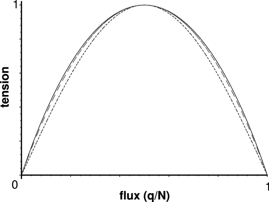
Figure 1: A plot of the $q$-string tension versus $q/N$. The solid, outermost line is the tension computed using the $\mathbf{Y}_{S}$ CGLP fractional D2-brane model. The dashed line corresponds to quadratic scaling, $q\,(N-q)$. The dotted line, farthest inside, is a sine law. The maximum tensions are normalized to one.

Figure 2: A plot of $T_{q}/T_{1}$ versus $q$ for an $SU(10)$ gauge theory. The diamonds were calculated using the $\mathbf{Y}_{S}$ fractional D2-brane model. The solid line corresponds to a quadratic scaling law. The dashed line comes from the sine scaling law.

3.2 Confining Strings and $\mathbb{CP}^{2}$

Although the $\mathbf{S}^{4}$ confining strings worked amazingly well, the confining strings involving $\mathbb{CP}^{2}$ remain murky. To try to give a balanced account, we present our results for this more ambiguous case.

We choose coordinates on $\mathbb{CP}^{2}$ where the Einstein metric is

$$ds^{2}=2\left(d\mu^{2}+\frac{1}{4}\sin(\mu)^{2}(\sigma_{1}^{2}+\sigma_{2}^{2}+\cos(\mu)^{2}\sigma_{3}^{2})\right)$$ (60)

and where

$$\sigma_{1}=d\theta\;;\;\;\;\sigma_{2}=\sin(\theta)d\phi\;;\;\;\;\sigma_{3}=(d\psi+\cos(\theta)d\phi)\ .$$ (61)

The coordinates $(\psi,\theta,\phi)$ are the Euler angles on a $\mathbf{S}^{3}$. We make an ansatz where the D4-branes wrap this squashed $\mathbf{S}^{3}$ sitting inside $\mathbb{CP}^{2}$. At the end, we will minimize the energy as a function of $\mu$. While rotational invariance of the $\mathbf{S}^{4}$ made choosing a three cycle relatively easy, it is not completely clear that this $\mathbf{S}^{3}\subset\mathbb{CP}^{2}$ is the best, in the sense of most stable, submanifold to choose.

The Lagrangian is

$${\mathcal{L}}=-A\sin(\mu)^{3}\cos(\mu)\sqrt{1-E^{2}}+QE\sin(\mu)^{4}\$$ (62)

where

$$A=\frac{\mu_{4}\lambda\ell^{3}}{g_{s}}2\pi^{2}\ ,\;\;\;Q=\frac{\mu_{4}\lambda\ell^{3}}{g_{s}}\frac{3\pi^{2}}{4a_{0}^{1/2}}\ .$$ (63)

The electric field $E$ is defined as in (48).

There is also a conserved momentum $P=d{\mathcal{L}}/dE$ quantized exactly as above. The Hamiltonian for the system is then

$$H=\sqrt{A^{2}\sin(\mu)^{6}\cos(\mu)^{2}+(P-Q\sin(\mu)^{4})^{2}}\ .$$ (64)

To minimize the Hamiltonian, one finds that $\mu$ must satisfy

$$(P-Q\sin(\mu)^{4})=\frac{A^{2}}{Q}\left(\frac{3}{4}\sin(\mu)^{2}-\sin(\mu)^{4}\right)\ .$$ (65)

This value of $\mu$ is indeed a minimum provided $A^{2}/Q^{2}<8/5$. Substituting this expression back into $H$, one finds that the minimum energy is

$$H_{min}=A\sin(\mu)^{2}\left[\left(\frac{A^{2}}{Q^{2}}-1\right)\sin(\mu)^{4}+\left(1-\frac{3A^{2}}{2Q^{2}}\right)\sin(\mu)^{2}+\frac{9A^{2}}{16Q^{2}}\right]^{1/2}\ .$$ (66)

The range of $\mu$ is $0\leq\mu\leq\pi/2$. Thus we see that while $H_{min}$ vanishes at $\mu=0$, it does not do so at $\mu=\pi/2$, precluding any $\mathbb{Z}_{2}$ symmetry.

This example is stranger still. The maximum value of $P/Q$ is

$$\left(\frac{P}{Q}\right)_{max}=1-\frac{A^{2}}{4Q^{2}}\ .$$ (67)

As $A/Q=8a_{0}^{1/2}/3=0.87201\ldots$, the maximum number of confining $q$-strings allowed is

$$q_{max}=N\left(1-\frac{A^{2}}{4Q^{2}}\right)\ ,$$ (68)

some noninteger number….

The problem may lie with our choice of a submanifold of $\mathbb{CP}^{2}$. We hope to return to this example in the future, armed with a better ansatz.

Appendix A First Order System

As a check of the fractional D2-brane solutions presented in section 2, we now present an independent derivation that makes use of an effective one dimensional action. We will see that this one dimensional action can be written in terms of a superpotential. Moreover, the metric and field strengths of the previous section derive from a first order system of differential equations arising from this superpotential. That the fractional D2-brane solution obeys a first order system of equations strengthens the claim of [4] that this supergravity solution does indeed preserve supersymmetry.

The idea is to start with the full type IIA supergravity Lagrangian

$$\frac{1}{2\kappa^{2}}\int d^{10}x(-G)^{1/2}R-\frac{1}{4\kappa^{2}}\int\biggl{(}d\phi\wedge*d\phi+g_{s}e^{-\Phi}H_{3}\wedge\star H_{3}$$

$$+g_{s}^{1/2}e^{3\phi/2}F_{2}\wedge\star F_{2}+g_{s}^{3/2}e^{\phi/2}\tilde{F}_{4}\wedge\star\tilde{F}_{4}+g_{s}^{2}B_{2}\wedge F_{4}\wedge F_{4}\biggr{)},$$ (69)

where

$$\tilde{F}_{4}=F_{4}-C_{1}\wedge H_{3}\;\;\;,\;\;\;F_{4}=dC_{3}\;\;\;,\;\;\;F_{2}=dC_{1}\ ,$$ (70)

and $2\kappa^{2}=(2\pi)^{7}{\alpha^{\prime}}^{4}g_{s}^{2}$.

We then make an ansatz for the metric and field strengths that depends on only one coordinate, namely the radius. The metric is

$$ds_{10}^{2}=e^{-5z}dx^{\mu}dx^{\nu}\eta_{\mu\nu}+e^{3z}ds_{7}^{2}$$ (71)

where $ds_{7}^{2}$ is as in (5). Thus the metric will depend on three undetermined functions $z(r)$, $h(r)$, $a(r)$, and $b(r)$. For convenience, we redefine

$$e^{u(r)}=a(r)\;;\;\;\;e^{v(r)}=b(r)\ .$$ (72)

The field strengths are then chosen to obey the Bianchi identities. The two form $F_{2}=0$. The dilaton is left as $\phi(r)$. The other forms are

$$\ell B_{2}=m\left(g_{1}(r)X_{2}+g_{2}(r)J_{2}\right)\ ,$$ (73)

and

$$g_{s}F_{4} = K(r)d^{3}x\wedge dr+2m(g_{3}(r)+c_{1})J_{2}\wedge J_{2}+2m(g_{3}(r)+c_{2})X_{2}\wedge J_{2}$$ (74)

$$+mg_{3}(r)^{\prime}\epsilon_{ijk}\mu^{i}dr\wedge D\mu^{j}\wedge J^{k}\$$

where $c_{1}$ and $c_{2}$ are integration constants.

After some algebra, the following one dimensional effective action emerges

$$S=\frac{\ell^{5}\mathrm{Vol}(M^{2,1})\mathrm{Vol}(M_{6})}{2\kappa^{2}}\int{\mathcal{L}}\,dr$$ (75)

where $M^{2,1}$ is the 2+1 dimensional Minkowski space and the $M^{6}$ are the level surfaces of the seven dimensional $G_{2}$ manifold. The Lagrangian is ${\mathcal{L}}=T-V$ where

$$T = \frac{e^{2u+4v}}{h}\left[-30(z^{\prime})^{2}+2(u^{\prime})^{2}+16u^{\prime}v^{\prime}+12(v^{\prime})^{2}-\frac{1}{2}(\phi^{\prime})^{2}\right.$$ (76)

$$-\frac{1}{2}\frac{m^{2}}{\ell^{6}}g_{s}e^{-\phi-6z}\left((g_{1}^{\prime})^{2}e^{-4u}+2(g_{2}^{\prime})e^{-4v}\right)$$

$$\left.-2\frac{m^{2}}{\ell^{6}}g_{s}^{-1/2}e^{\phi/2-9z-2u-4v}(g_{3}^{\prime})^{2}\right]$$

and

$$V = he^{-2u-4v}\left[2e^{2u+8v}-2e^{6u+4v}+12e^{4u+6v}-2\frac{m^{2}}{\ell^{6}}g_{s}e^{-\phi-6z+2u+4v}(g_{1}+g_{2})^{2}\right.$$ (77)

$$\left.-4\frac{m^{2}}{\ell^{6}}g_{s}^{-1/2}e^{\phi/2-9z}\left(2(g_{3}+c_{1})^{2}e^{4u}+(g_{3}+c_{2})^{2}e^{4v}\right)\right]$$

$$-\frac{1}{2}g_{s}^{-1/2}e^{\phi/2+15z+2u+4v}h^{-1}K^{2}+\frac{4m^{2}}{\ell^{6}}K\left[g_{3}(g_{1}+g_{2})+g_{1}c_{1}+g_{2}c_{2}\right]\ .$$

Notice that the functions $h(r)$ and $K(r)$ are non-dynamical. We leave $h(r)$ in the Lagrangian in order to retain reparametrization invariance. After all, we eventually hope to identify $r$ with the radius of section 2. The Lagrangian simplifies a little if we solve for the minimum value of $K(r)$ and replace the old Lagrangian with a new one evaluated at this minimum:

$$K(r)=\frac{4m^{2}}{\ell^{6}}g_{s}^{1/2}e^{-\phi/2-15z-2u-4v}h\left[g_{3}(g_{1}+g_{2})+g_{1}c_{1}+g_{2}c_{2}\right]\ .$$ (78)

Having made this replacement, the potential becomes

$$V\rightarrow-he^{-2u-4v}\left[2e^{2u+8v}-2e^{6u+4v}+12e^{4u+6v}-2\frac{m^{2}}{\ell^{6}}g_{s}e^{-\phi-6z+2u+4v}(g_{1}+g_{2})^{2}\right.$$

$$\left.-4\frac{m^{2}}{\ell^{6}}g_{s}^{-1/2}e^{\phi/2-9z}\left(2(g_{3}+c_{1})^{2}e^{4u}+(g_{3}+c_{2})^{2}e^{4v}\right)\right]$$

$$+\frac{8m^{2}}{\ell^{12}}g_{s}^{1/2}e^{-\phi/2-15z-2u-4v}h\left[g_{3}(g_{1}+g_{2})+g_{1}c_{1}+g_{2}c_{2}\right]^{2}\ .$$ (79)

This Lagrangian can be written in terms of a superpotential. Indeed, let

$$T=G_{ab}\dot{\varphi}^{a}\dot{\varphi}^{b}$$ (80)

where the $\varphi^{a}$ correspond to the functions $u$, $v$, $z$, $\phi$, and $g_{i}$, and the dot means differentiation with respect to the radius $r$. The $h^{\prime}$, as $h$ is nondynamical, does not appear in $T$. In this notation, the potential can be written as

$$V=-G^{ab}\frac{\partial W}{\partial\varphi^{a}}\frac{\partial W}{\partial\varphi^{b}}$$ (81)

where $G^{ab}$ is the inverse of $G_{ab}$ and

$$W=2\left[e^{u+4v}+e^{3u+2v}-\frac{m^{2}}{\ell^{6}}g_{s}^{1/4}e^{-\phi/4-15z/2}\left(g_{3}(g_{1}+g_{2})+c_{1}g_{1}+c_{2}g_{2}\right)\right]\ .$$ (82)

The existence of the superpotential $W$ implies that

$${\mathcal{L}}=G_{ab}\left(\dot{\varphi}^{a}-G^{ac}\frac{\partial W}{\partial\varphi^{c}}\right)\left(\dot{\varphi}^{b}-G^{bd}\frac{\partial W}{\partial\varphi^{d}}\right)+2\frac{dW}{dr}\ .$$ (83)

In this way, a simple set of first order, differential equations emerges,

$$\dot{\varphi}^{a}=G^{ab}\frac{\partial W}{\partial\varphi^{b}}\ .$$ (84)

It is straightforward now to make sure that the metric functions and field strengths of section 2 satisfy this system of first order equations. One easy observation is that $2z^{\prime}=\phi^{\prime}$. This observation is equivalent to the statement that the warp factor $H(r)^{1/4}\equiv e^{2z}=g_{s}^{-1}e^{\phi(r)}$ noted earlier. With this substitution, the first order system becomes:

$$u^{\prime}/h = \left(e^{-u}-e^{u-2v}\right)\ ,$$ (85)

$$v^{\prime}/h = e^{2u-2v}\ ,$$ (86)

$$z^{\prime}/h = -\frac{m^{2}}{2\ell^{6}}e^{-2u-4v-8z}\left(g_{3}(g_{1}+g_{2})+c_{1}g_{1}+c_{2}g_{2}\right)\ ,$$ (87)

$$g_{1}^{\prime}/h = 4(g_{3}+c_{1})e^{2u-4v}\ ,$$ (88)

$$g_{2}^{\prime}/h = 2(g_{3}+c_{2})e^{-2u}\ ,$$ (89)

$$g_{3}^{\prime}/h = (g_{1}+g_{2})\ .$$ (90)

As promised, the $h$ allows us some freedom in the choice of $r$. It is convenient to choose $h(r)$ as in (7). It is then straightforward to see that $a(r)$ and $b(r)$ of section 2 satisfy the first pair of equations in the first order system.

The last four differential equations have a simple interpretation. The last three differential equations constitute a geometric condition on the forms. They enforce the condition that $G_{3}=\star_{7}G_{4}$ where $\star_{7}$ is the Hodge dual with respect to the $G_{2}$ manifold. As discussed in the text, the equation for the warp factor (87) corresponds to the integrated equation of motion for the four form field strength $F_{4}$.

We present a few details necessary to integrate (87). The relations between the $f_{i}$ of the previous section and the $g_{i}$ are as follows:

$$g_{1}^{\prime}=f_{1}\;;\;\;\;g_{2}^{\prime}=f_{2}\;;\;\;\;g_{3}^{\prime}=hf_{3}\;.$$ (91)

Now the $f_{i}$ depend on elliptic integrals and the reader might expect that the $g_{i}$ can at best be expressed as double integrals. It is surprising but true that the $g_{i}$ are no more complicated than the $f_{i}$. Indeed

$$g_{1}=-8a^{2}b^{2}f_{3}\;;\;\;\;g_{2}=(1+8a^{2}b^{2})f_{3}\ .$$ (92)

The function $g_{3}$ can be expressed in terms of $f_{1}$ or $f_{2}$ using either (88) or (89), giving a relation between the integration constants $32(c_{1}-c_{2})=3$. (Note that we are free to change $g_{3}$ by a constant without changing the solution; the geometry does not specify both $c_{1}$ and $c_{2}$, only the difference.)

After some algebra, we find that

$$H(r)=\frac{m^{2}}{2\ell^{6}}\int_{r}^{\infty}\rho\left(2u_{2}(\rho)u_{3}(\rho)-3u_{3}(\rho)\right)d\rho\ .$$ (93)

References

- [1] J. Maldacena, “The Large N limit of superconformal field theories and supergravity,” Adv. Theor. Math. Phys. 2 (1998) 231, hep-th/9711200.
- [2] S. S. Gubser, I. R. Klebanov, and A. M. Polyakov, “Gauge theory correlators from noncritical string theory,” Phys. Lett. B428 (1998) 105, hep-th/9802109.
- [3] E. Witten, “Anti-de Sitter space and holography,” Adv. Theor. Math. Phys. 2 (1998) 253, hep-th/9802150.
- [4] M. Cvetič, G. W. Gibbons, H. Lü, and C. N. Pope, “Supersymmetric Non-singular Fractional D2-branes and NS-NS 2-branes,” Nucl. Phys. B 606 (2001) 18, hep-th/0101096
- [5] I. R. Klebanov and M. Strassler, “Supergravity and a Confining Gauge Theory: Duality Cascades and SB–Resolution of Naked Singularities,” JHEP 0008 (2000) 052, hep-th/0007191.
- [6] I. R. Klebanov and E. Witten, “Superconformal field theory on three-branes at a Calabi-Yau singularity,” Nucl. Phys. B536 (1998) 199, hep-th/9807080; A. Kehagias, “New Type IIB Vacua and Their F-Theory Interpretation,” Phys. Lett. B435 (1998) 337, hep-th/9805131; D. Morrison and R. Plesser, “Non-Spherical Horizons, I,” Adv. Theor. Math. Phys. 3 (1999) 1, hep-th/9810201.
- [7] I. R. Klebanov and N. Nekrasov, “Gravity Duals of Fractional Branes and Logarithmic RG Flow,” Nucl. Phys. B574 (2000) 263, hep-th/9911096.
- [8] I. R. Klebanov and A. Tseytlin, “Gravity Duals of Supersymmetric Gauge Theories,” Nucl. Phys. B574 (2000) 123, hep-th/0002159.
- [9] M. Cvetič, G. W. Gibbons, H. Lu and C. N. Pope, “Ricci-flat metrics, harmonic forms and brane resolutions,” hep-th/0012011.
- [10] C. P. Herzog and I. R. Klebanov, “Gravity duals of fractional branes in various dimensions,” Phys. Rev. D 63 (2001) 126005, hep-th/0101020.
- [11] A. Loewy and Y. Oz, “Branes in Special Holonomy Backgrounds,” hep-th/0203092.
- [12] C. P. Herzog and I. R. Klebanov, “On String Tensions in Supersymmetric Gauge Theory,” Phys. Lett. B 526 388, hep-th/0111078.
- [13] G. W. Gibbons, D. N. Page, and C. N. Pope, “Einstein Metrics on , , and Bundles,” Comm. Math. Phys. 127 (1990) 529.
- [14] J. Ambjorn, P. Olesen and C. Peterson, “Three-Dimensional Lattice Gauge Theory And Strings,” Nucl. Phys. B 244 (1984) 262; “Observation Of A String In Three-Dimensional SU(2) Lattice Gauge Theory,” Phys. Lett. B 142 (1984) 410; “Stochastic Confinement And Dimensional Reduction. 1. Four-Dimensional SU(2) Lattice Gauge Theory,” Nucl. Phys. B 240 (1984) 189.
- [15] B. Lucini and M. Teper, “Confining strings in SU(N) gauge theories,” Phys. Rev. D64 (2001) 105019, hep-lat/0107007.
- [16] C. G. Callan, A. Guijosa, K. G. Savvidy and O. Tafjord, “Baryons and flux tubes in confining gauge theories from brane actions,” Nucl. Phys. B555 (1999) 183, hep-th/9902197.
- [17] M. R. Douglas and S. H. Shenker, “Dynamics of SU(N) supersymmetric gauge theory,” Nucl. Phys. B447 (1995) 271, hep-th/9503163.
- [18] A. Hanany, M. J. Strassler and A. Zaffaroni, “Confinement and strings in MQCD,” Nucl. Phys. B513 (1998) 87, hep-th/9707244.
- [19] L. Del Debbio, H. Panagopoulos, P. Rossi and E. Vicari, “Spectrum of confining strings in SU(N) gauge theories,” JHEP 0201 (2002) 009, hep-th/0111090.
- [20] J. D. Edelstein, W. G. Fuertes, J. Mas and J. M. Guilarte, “Phases of dual superconductivity and confinement in softly broken N = 2 supersymmetric Yang-Mills theories,” Phys. Rev. D62 (2000) 065008, hep-th/0001184.
- [21] M. J. Strassler, “Messages for QCD from the Superworld,” Prog. Theor. Phys. Suppl. 131 (1998) 439, hep-lat/9803009.
- [22] J. M. Maldacena and H. Nastase, “The supergravity dual of a theory with dynamical supersymmetry breaking,” JHEP 0109 (2001) 024, hep-th/0105049.
- [23] C. Herzog, I. R. Klebanov and P. Ouyang, “Remarks on the Warped Deformed Conifold,” hep-th/0108101.
- [24] B. S. Acharya, J. M. Figueroa-O’Farrill, C. M. Hull and B. Spence, “Branes at conical singularities and holography,” Adv. Theor. Math. Phys. 2 (1999) 1249, hep-th/9808014.
- [25] R. Myers, “Dielectric Branes,” JHEP 9912 (1999) 022, hep-th/9910053.
- [26] C. G. Callan and I. R. Klebanov, “D-Brane Boundary State Dynamics,” Nucl. Phys. B 465 (1996) 473, hep-th/9511173.
- [27] E. Witten, “Supersymmetric index of three-dimensional gauge theory,” hep-th/9903005.