Inflationary cosmology in the
central region of String/M-theory moduli space

Abstract

The “central” region of moduli space of M- and string theories is where the string coupling is about unity and the volume of compact dimensions is about the string volume. Here we argue that in this region the non-perturbative potential which is suggested by membrane instanton effects has the correct scaling and shape to allow for enough slow-roll inflation, and to produce the correct amplitude of CMB anisotropies. Thus, the well known theoretical obstacles for achieving viable slow-roll inflation in the framework of perturbative string theory are overcome. Limited knowledge of some generic properties of the induced potential is sufficient to determine the simplest type of consistent inflationary model and its predictions about the spectrum of cosmic microwave background anisotropies: a red spectrum of scalar perturbations, and negligible amount of tensor perturbations.

Attempts to obtain viable inflationary cosmology in the framework of string/M-theory have encountered notorious difficulties. In particular, potentials are typically too steep, so they cannot provide enough slow-roll inflationBG ; BS ; BBSMS , and models of “fast-roll” inflationPBB have difficulty in reproducing the observed spectrum of CMB anisotropiesMVDV .

In bda2 a scenario for stabilization of string- and M-theoretic moduli in the central region of moduli space was proposed. In this scenario, the central region is parameterized by chiral superfields of D=4, $N=1$ Supergravity (SUGRA), which are all stabilized at the string scale by stringy non-perturbative (SNP) effects induced by membrane instantons bda1 . Supersymmetry (SUSY) is broken at a lower intermediate scale by field theoretic effects that shift the stabilized moduli only by a small amount from their unbroken minima. The cosmological constant can be made to vanish after SUSY breaking if there is an adjustable constant of stringy origin.

Here we show that this scenario can accommodate slow-roll inflation without unnatural tuning of potential parameters, thus overcoming the aforementioned difficulties. The simplest consistent inflation model is that of topological inflation vilenkin ; BBSMS , in which inflating domain walls are formed at the top of the barrier separating the central region from the outer (perturbative) region of moduli space, and subsequently the field roles down to the SUSY preserving minimum in the central region and inflation ends. We find a model that predicts a spectral index of scalar perturbations that is less than unity, that has a negligible amount of tensor perturbations, and that provides an opportunity for the use of measurements of CMB anisotropies as a probe of central region moduli dynamics.

The moduli potential is an important ingredient in any string theoretic cosmological scenario. So any argument which ignores the question of moduli stabilization fails to address an important cosmological issue and its conclusions are suspect. The usual mechanisms which generate moduli potentials in the perturbative regions of moduli space give runaway (or steep) potentials that vitiate many conclusions coming from models of brane annihilation, tachyon condensation and Ekpyrosis. We will discuss problems with such scenarios and the possible evolution from the outer perturbative regions to the central region separatelybdn . The point of this paper is that the mechanism that one might expect to exist in the central region to stabilize the moduli will also generate sufficient inflation and lead to an acceptable CMB spectrum. So any additional inflationary mechanism is redundant.

To determine the size of the central region we need to determine the correct normalization of moduli kinetic terms. We follow an argument which was first made by Banks banks in the context of Horava-Witten (HW) theory in the outer region of moduli space. In the effective 4D theory obtained after compactification of 10D string theories on a compact volume $V_{6}$, moduli kinetic terms are multiplied by compact volume factors $M_{S}^{8}V_{6}$ ($M_{S}$ being the string mass), and $M_{11}^{9}V_{7}$ in M-theory compactifications ($M_{11}$ being the M-theory scale and $V_{7}$ the compact volume). The curvature term in the effective 4D action is multiplied by the same volume factors. We may use the 4D Newton’s constant $8\pi G_{N}=m_{p}^{-2}$ to “calibrate” moduli kinetic terms, and determine that they are multiplied by factors of the 4D (reduced) Planck mass squared, $\Gamma=\int d^{4}x\left\{\frac{m_{p}^{2}}{2}\sqrt{-g}R+\frac{m_{p}^{2}}{2}\partial\psi\partial\psi\right\}$. This argument holds for all string/$M$-theory compactifications.

Strictly speaking, the argument we have presented can be expected to be somewhat modified in the central region, perhaps by different factors of order unity multiplying the curvature and moduli kinetic terms. But the effective 4D theory must always take the form of $\Gamma$ with some SUGRA potential. Using this scaling, we find that the typical distances over which the moduli can move within field space, while remaining within the central region, should be a number of order one in units of $m_{p}$.

We argue that the overall scale of the moduli potential is $\Lambda^{4}=M_{S}^{6}/m_{p}^{2}$ in compactifications of string theories and $\Lambda^{4}=M_{11}^{6}/m_{p}^{2}$ in compactifications of $M$-theory. Of course, in the central region we expect that $M_{S}\sim M_{11}$. First, the overall scale of the superpotential is $M_{S}^{3}$ in string theory compactifications and $M^{3}_{11}$ for $M$-theory compactifications. The key point here is that there are no additional volume factors coming from some or all of the compact dimensions. This was first noticed in the context of outer region compactifications of HWbanks . Banks argued that the superpotential is generated on the 4D branes, and that since the superpotential is generated only in 4D theories, it cannot depend on the compactification volume which is a higher dimensional object. Note that this scaling argument is very general and applies to the central region as well. Any additional volume factors multiplying $M_{S}^{3}$ could only result from the existence of zero-modes associated with the embedding of the wrapped Euclidean brane in the compact space. However, such zero-modes will necessarily enhance the number of SUSY’s in the effective 4D theory, and so by non-renormalization theorems a superpotential could not be generated. A superpotential of order $M^{3}_{S/11}$ will in turn produce a potential of order $\Lambda^{4}=M_{S/11}^{6}/m_{p}^{2}$.

Our argument is supported by existing explicit calculations of the non-perturbative superpotential induced by brane instantons HM ; Moore ; Ovrut . There the induced potential is calculated by comparing a gravitino correlator in the background of the brane instanton to an effective theory with instanton effects integrated out. The comparison shows that the prefactor contains only factors associated with topological properties of the compact space.

Let us give two representative examples, type I string theory and HW theory. We can perform analogous calculations in other backgrounds, or simply use the duality relations connecting them. The numerical relations are taken from bda1 . Consider type I string theory compactified on a 6D manifold. The string length is denoted by $l_{I}$, the string coupling by $g$, and the compact 6D volume by $V=(2\pi R)^{6}$. The string scale $M_{S}$ in type I theory is related to $l_{I}$ by $M_{S}^{8}=2(2\pi)^{-7}l_{I}^{-8}$, the 4D Newton’s constant is given by $G_{N}=\frac{1}{8}g^{2}l_{I}^{8}R^{-6}$ and the Yang-Mills coupling by $\alpha_{YM}=\frac{1}{2}gl_{I}^{6}R^{-6}$. These are related by $G_{N}/\alpha_{YM}=\frac{1}{4}gl_{I}^{2}$; therefore the string length is given by $l_{I}=2(g~{}\alpha_{YM}~{}8\pi m_{p}^{2})^{-1/2}$, and the string mass by $M_{S}=(4\pi)^{-7/8}(g~{}\alpha_{YM}~{}8\pi m_{p}^{2})^{1/2}$. Putting $m_{p}=2.4\times 10^{18}GeV$, we obtain an estimate for the string mass in type I string theory of $M_{S}=2.6\times 10^{17}GeV\sqrt{\alpha_{YM}/(1/25)}\sqrt{g}$. Since we have defined $\Lambda^{4}=M_{S}^{6}m_{p}^{-2}$, our estimate for the moduli potential scale $\Lambda$ in type I theory is

$$\Lambda_{I}=8.6\times 10^{16}GeV\left(\frac{\alpha_{YM}}{(1/25)}\right)^{3/4}g^{3/4}.$$ (1)

Now consider compactifications of HW theory. The size of the 11 dimension interval is $\pi\rho$, and the compact 6 volume is $V=a^{6}$. The 11D Planck mass $M_{11}$ is related to the 11D gravitational constant by $\kappa_{11}^{2}=M_{11}^{-9}$. The 4D Newton’s constant is given by $G_{N}=\frac{1}{8\pi^{2}}\kappa_{11}^{2}a^{-6}\rho^{-1}$ and $\alpha_{YM}=\frac{1}{2}(4\pi\kappa_{11}^{2})^{2/3}a^{-6}$, so that $M_{11}=(4\pi)^{1/9}(2\alpha_{YM})^{-1/6}a^{-1}$. Putting in numbers we find that $M_{11}\simeq 2\left(\alpha_{YM}/(1/25)\right)^{-1/6}\frac{1}{M_{GUT}a}M_{GUT}$. Taking $M_{GUT}=3\times 10^{16}$ GeV, $M_{GUT}a\sim.25-1$, allows $M_{11}\pi\rho\sim 1$ which means that the string coupling is of order unity, $g\sim 1$, and $M_{11}\stackrel{{\scriptstyle>}}{{{}_{\sim}}}M_{GUT}$. So our estimate for the string mass in central region compactifications of HW theory is $M_{11}=2.4\times 10^{17}GeV\frac{1}{4M_{GUT}a}\left(\alpha_{YM}/(1/25)\right)^{-1/6}$, and since the potential scales as $\Lambda^{4}=M_{11}^{6}m_{p}^{-2}$ we obtain

$$\Lambda_{HW}\!=\!7.6\!\times\!10^{16}{\rm GeV}\!\left(4M_{GUT}a\right)^{-3/2}\!\left(\frac{\alpha_{YM}}{(1/25)}\right)^{-1/4}.$$ (2)

With $\alpha_{YM}\!\sim\!1/25$ at the GUT scale and $M_{GUT}a\!\sim\!1$ we have $M_{11}\!\sim\!M_{S}\sim\!10^{17}$GeV, and $\Lambda_{I}\!\sim\!\Lambda_{HW}\!\sim\!10^{16}$ GeV.

Let us consider the expected form of the superpotential in the central region based on the picture discussed in bda1 . The theory in each corner of moduli space has non-perturbative effects that originate from various Euclidean branes wrapping on cycles of the compact space. However, in the outer region they will only give runaway potentials that take the theory to the zero coupling and decompactification limit. On the other hand every perturbative theory has strong coupling (S-dual) and small compact volume (T-dual) partners. From the point of view of one perturbative theory, the potential in the dual theory is trying to send the original theory to the strong coupling and/or zero compact volume limit. Thus it would seem that in the universal effective field theory in the central region there are competing terms in the potential. If the signs of the prefactors are the same and (as expected) are of similar magnitude, the potential would contain a minimum at $g\sim O(1)$ and the size of the internal manifold would be of the order of the string scale.

To illustrate this consider the S-dual type I and Heterotic SO(32) (I-HO) theories. The S-duality relations between them are $\phi_{I}=-\phi_{HO}$, $g_{I}=\frac{1}{g_{H}}$, $l_{I}^{2}=g_{HO}l^{2}_{HO}$. The string coupling is related to the expectation value of the dilaton by $g=\langle e^{\phi}\rangle$, and $l_{I,HO}$ refers to the string length in I/HO theories, respectively. Note that the relation between scales is defined in terms of the expectation value of the (stabilized) dilaton. In this case terms in the superpotential $W$ come from a Euclidean $D_{5}$ brane wrapping the whole compact six space, or a Euclidean $D_{1}$ wrapping a one cycle in the compact six-space on the type I side, and a Euclidean $F_{5}$ brane wrapping the whole compact six space, or a Euclidean $F_{1}$ brane wrapping a one cycle in the compact six-space on the HO side. The leading order expressions (up to pre-factors whose size we have estimated to be $M_{S}^{3}$) for these can be read off from table II of bda1 .

In the central region we then expect both these competing effects to be present(we hope to discuss this more concretely in a future publication). As explained in bda2 , the minimum should be supersymmetric $W^{\prime}=W=0$, where the latter may happen, for instance, if there is an R-symmetry under which W has an R-charge of 2 BBSMS .

The moduli potential originates from brane instantons which depend exponentially on string coupling $g$, or on the size of the 11D interval or circle $\rho/l_{11}$, and on compactification radii $R/l_{s}$, as we have just described. Calling them generically $\psi$, the 4D action takes the form $\Gamma=\int d^{4}x\left\{\frac{1}{2}m_{p}^{2}\partial\psi\partial\psi-\Lambda^{4}v(\psi)\right\}.$ The overall scale of the potential was estimated previously as $\Lambda=M_{S}^{3/2}m_{p}^{-1/2}$, and the potential $v(\psi)$ can be approximated in the central region by a polynomial function. Canonically normalizing the moduli in order to later compare to models of inflation we define $\phi=m_{p}\psi$, and obtain $\Gamma=\int d^{4}x\left\{\frac{1}{2}\partial\phi\partial\phi-\Lambda^{4}v(\phi/m_{p})\right\}.$

By assumption, the moduli potential has a SUSY preserving minimum where it vanishes in the central region. Additionally, it has to vanish at infinity (the extreme outer parts of moduli space), since there the non-perturbative effects vanish exponentially, and the 10D/11D SUSY is restored. Since $v(\phi)$ vanishes at the minimum in the central region and $v(\phi)$ vanishes at infinity, its derivative $\delta v/\delta\phi$ needs to vanish somewhere in between. Since the potential is increasing in all directions away from the minimum in the central region, that additional extremum needs to be a maximum.

This means that in any direction there is at least one maximum separating the central region and the outer region. As we discussed, the distance of this maximum from the minimum is a number of order one in units of $m_{p}$. Note that since we are dealing with multidimensional moduli space the maxima in different directions do not need to coincide, so in general they are saddle points, but we focus on a single direction in field space. The simplest models without additional tuning of the parameters will not have additional stable local minima with non-vanishing energy density. This would require tuning of four coefficients in the superpotential (or Kahler potential).

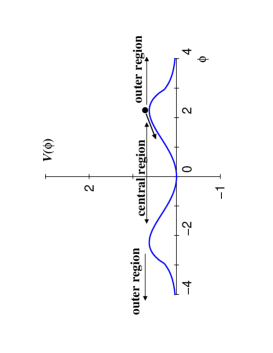
Figure 1: An example of the expected form of the moduli potential in the central region of moduli space. Shown are the SUSY preserving minimum at $\phi=0$ (arbitrary choice), and the maximum near $\phi=2$. The inflaton rolls from the top of the barrier to the minimum as indicated. $V(\phi)$ is in units of $M_{S}^{6}m_{p}^{-2}$ and $\phi$ is in units of $m_{p}$.

The simplest model of central region inflation is that of topological inflation from the top of the barrier between the central and outer region. If initially the field is randomly distributed and can settle down on either side of the barrier, then typically some inflating domain wall will be produced vilenkin (see also BBSMS ). Calling the thickness (in configuration space) of the wall $\delta$, and the distance (in field space) between the central and outer region minima $\Delta$, then the balance between gradient and potential energies requires that $\left(\frac{\Delta}{\delta}\right)^{2}\simeq\Lambda^{4}$. Einstein’s equation relates the Hubble parameter $H$ and $\Lambda$ by $H^{2}=\frac{1}{3m_{p}^{2}}\Lambda^{4}$. According to vilenkin an inflating domain wall will be produced provided that its width is comparable to the horizon size $H^{-1}$, that is $\delta H\stackrel{{\scriptstyle>}}{{{}_{\sim}}}1$. This requirement is then equivalent to $\Delta\stackrel{{\scriptstyle>}}{{{}_{\sim}}}m_{p}$, which is clearly satisfied in the case at hand. The previous line of reasoning shows that generic initial conditions indeed produce inflating regions. At the end of inflation the inflaton field settles into its central region SUSY preserving minimum.

We now wish to show that the model we are proposing can produce enough inflation to resolve the cosmological problems that inflation is supposed to resolve. The potential near the maximum of the barrier at $\phi=\phi_{\rm max}$ can be approximated by the form $\Lambda^{4}\left[1-(\frac{\phi-\phi_{max}}{\mu})^{2}\right]$, with $\mu^{2}=\frac{2m_{p}^{2}}{|v^{\prime\prime}(\phi_{\rm max})|}$. We recognize this model as a “small single field” $p=2$ inflation model according to the classification of kinney1 . This model is similar in many of its phenomenological consequences to “natural inflation” natural .

Recall the definitions of the slow roll parameters ( we use the conventions of kolb ; kinney1 ; kinney2 except that we use the reduced Planck mass $m_{P}^{2}=1/(8\pi G_{N}$)), $\epsilon=\frac{m_{p}^{2}}{2}\left(\frac{V^{\prime}}{V}\right)^{2}$, and $\eta={m_{p}^{2}}\left(\frac{V^{\prime\prime}}{V}\right)-\frac{m_{p}^{2}}{2}\left(\frac{V^{\prime}}{V}\right)^{2}$. The end of inflation is reached when $\epsilon=1$, and the number of inflationary e-folds is given by

$$N(\phi,\phi_{\rm end})=\frac{1}{\sqrt{2}m_{p}}\int\limits_{\phi}^{\phi_{\rm end}}\frac{1}{\sqrt{\epsilon(\phi)}}d\phi.$$ (3)

For our particular case $\sqrt{\epsilon(\phi)}=-\sqrt{2}\frac{m_{p}}{\mu^{2}}\frac{\phi-\phi_{\rm max}}{1-\left(\frac{\phi-\phi_{\rm max}}{\mu}\right)^{2}}$. The slow-roll conditions are obeyed if the slow roll parameters are small, which near the top of the potential they indeed are $\epsilon\sim 2\frac{m_{p}^{2}}{\mu^{4}}(\phi-\phi_{\rm max})^{2}$ and $\eta\sim v^{\prime\prime}(\phi_{\rm max})$, provided that $v^{\prime\prime}(\phi_{\rm max})$ is small enough (see below).

Since the required number of e-folds to resolve the cosmological problems is about 60, the initial value of the field needs to be close enough to the maximum of the potential such that $N(\phi_{\rm initial},\phi_{\rm end})\stackrel{{\scriptstyle>}}{{{}_{\sim}}}60$. Integrating eq.(3), assuming that $\phi_{\rm end}\sim\mu$ we obtain $\phi_{\rm initial}-\phi_{\rm max}\simeq\mu e^{-\left[120\left(\frac{m_{p}}{\mu}\right)^{2}\right]}$. The strongest constraint comes from requiring that quantum fluctuations are not larger than this estimate. The strength of quantum fluctuations is $\delta\phi\sim\frac{H}{2\pi}$, which implies that $\frac{\mu}{m_{p}}e^{-\left[120\left(\frac{m_{p}}{\mu}\right)^{2}\right]}\stackrel{{\scriptstyle>}}{{{}_{\sim}}}\frac{1}{2\pi}\frac{\Lambda^{2}}{m_{p}^{2}}$, where we have used $H^{2}=\frac{1}{3m_{p}^{2}}\Lambda^{4}$. This constraint can be satisfied provided that $\left(\frac{m_{p}}{\mu}\right)^{2}\stackrel{{\scriptstyle<}}{{{}_{\sim}}}1/10$, that is provided that $v^{\prime\prime}(\phi_{\rm max})\stackrel{{\scriptstyle<}}{{{}_{\sim}}}1/6$.

The amplitude of CMB anisotropies can be obtained by standard use of the slow roll equations, which lead to $P_{\zeta}^{1/2}\!=\!\frac{15}{2}\frac{\delta\rho}{\rho}\!=\!{\frac{\sqrt{3}}{2\pi}}\frac{1}{m_{p}^{3}}\frac{V^{3/2}}{V^{\prime}}\!\simeq\!10^{-4}$. Following kinney1 we integrate eq.(3), assuming $\phi_{end}\!\sim\!\mu$ to obtain $\phi_{CMB}\!=\!\mu e^{-\left[100\left(\frac{m_{p}}{\mu}\right)^{2}\right]}$, where $\phi_{\rm CMB}$ is defined by $N(\phi_{\rm CMB},\phi_{\rm end})\!=\!50$. Therefore $P_{\zeta}^{1/2}\!=\!\frac{\sqrt{3}}{4\pi}\frac{\mu\Lambda^{2}}{m_{p}^{3}}e^{\left[{100}\left(\frac{m_{p}}{\mu}\right)^{2}\right]}$, so that $\Lambda^{2}\!=\!\frac{4\pi}{\sqrt{3}}P_{\zeta}^{1/2}\frac{m_{p}^{3}}{\mu}e^{-\left[{100}\left(\frac{m_{p}}{\mu}\right)^{2}\right]}$. Putting numbers, and restoring explicitly the dependence on $v^{\prime\prime}(\phi_{\rm max})$ we obtain

$$\Lambda\simeq 6.5\times 10^{16}GeV\left(\frac{|v^{\prime\prime}(\phi_{\rm max})|}{2}\right)^{1/4}e^{-25|v^{\prime\prime}(\phi_{\rm max})|}.$$ (4)

So for consistency with our estimates in eqs.(1),(2) we need that $|v^{\prime\prime}(\phi_{\rm max})|\sim O(1/25)$, a little stronger than the condition that guarantees a sufficient amount of inflation which we have encountered previously. This is not a technically unnatural fine tuning since the gauge coupling at this point is of the same order.

The index of scalar perturbations is given by $n_{s}=1-4\epsilon_{\rm CMB}+2\eta_{CMB}$ and the tensor to scalar ratio is given by $r=13.7\epsilon_{\rm CMB}$. For our model $\epsilon_{CMB}$ is extremely small, and $\eta_{CMB}\simeq v^{\prime\prime}(\phi_{\rm max})$. Consequently,

$$n_{S} = .92-.08(25|v^{\prime\prime}(\phi_{max})|-1)$$

$$r \simeq 0.$$ (5)

Taking as a reasonable range $1/3\stackrel{{\scriptstyle<}}{{{}_{\sim}}}25|v^{\prime\prime}(\phi_{max})|\stackrel{{\scriptstyle<}}{{{}_{\sim}}}3$ we estimate $.76\leq n_{S}\leq.97$. This is within the range of allowed models based on current CMB anisotropy data and can be verified or falsified by more accurate data.

Detailed and accurate calculations of the non-perturbative potential in the central region are not yet available and have to await improvements in calculation techniques in string theory. In this context measurements of CMB anisotropies can be a useful guide to theory.

It is not likely that simple “large field” inflationary models in the central region are viable, since the central region cannot accommodate large motions of the inflaton. For example kinney1 , if the potential is $(\phi/m_{p})^{p}$, the inflaton field $\phi$ needs to move at least $\Delta(\phi^{2})=m_{p}^{2}100p$. Assuming that $\Delta\phi\sim\phi$, $\Delta\phi\sim 10\sqrt{p}\ m_{p}$. This is already too large for $p=2$, since this requires a central region size of at least about $30m_{p}$, which is unlikely. If CMB anisotropy data selects large field models (currently disfavored by the data kinney2 ) then all simple models of central region inflation will be ruled out.

This research is supported by grant 1999071 from the United States-Israel Binational Science Foundation (BSF), Jerusalem, Israel. SdA is supported in part by the United States Department of Energy under grant DE-FG02-91-ER-40672. EN is supported in part by a grant from the budgeting and planning committee of the Israeli council for higher education.

References

- (1) P. Binetruy and M. K. Gaillard, Phys. Rev. D 34, 3069 (1986).
- (2) R. Brustein and P. J. Steinhardt, Phys. Lett. B 302, 196 (1993).
- (3) T. Banks, M. Berkooz, S. H. Shenker, G. W. Moore and P. J. Steinhardt, Phys. Rev. D 52, 3548 (1995).
- (4) G. Veneziano, hep-th/9902097.
- (5) A. Melchiorri, F. Vernizzi, R. Durrer and G. Veneziano, Phys. Rev. Lett. 83, 4464 (1999).
- (6) R. Brustein and S. P. de Alwis, Phys. Rev. Lett. 87, 231601 (2001).
- (7) R. Brustein and S. P. de Alwis, Phys. Rev. D 64, 046004 (2001).
- (8) A. Vilenkin, Phys. Rev. Lett. 72, 3137 (1994).
- (9) R. Brustein, S. P. de Alwis and E. Novak, in preparation.
- (10) T. Banks, hep-th/9906126.
- (11) J. A. Harvey and G. W. Moore, hep-th/9907026.
- (12) G. W. Moore, G. Peradze and N. Saulina, Nucl. Phys. B 607, 117 (2001).
- (13) E. Lima, B. Ovrut, J. Park and R. Reinbacher, Nucl. Phys. B 614, 117 (2001).
- (14) F. C. Adams, J. R. Bond, K. Freese, J. A. Frieman and A. V. Olinto, Phys. Rev. D 47, 426 (1993).
- (15) J. E. Lidsey, A. R. Liddle, E. W. Kolb, E. J. Copeland, T. Barreiro and M. Abney, Rev. Mod. Phys. 69, 373 (1997).
- (16) S. Dodelson, W. H. Kinney and E. W. Kolb, Phys. Rev. D 56, 3207 (1997).
- (17) W. H. Kinney, A. Melchiorri and A. Riotto, Phys. Rev. D 63, 023505 (2001).