hep-th/0205033
AEI 2002-036

The metric of a spacetime with a parallel plane (pp)-wave can be obtained in a certain limit of the space AdS${}^{5}\times$S⁵. According to the AdS/CFT correspondence, the holographic dual of superstring theory on that background should be the analogous limit of ${\cal N}=4$ supersymmetric Yang-Mills theory. In this paper we shall show that, contrary to widespread expectation, non-planar diagrams survive this limiting procedure in the gauge theory. Using matrix model techniques as well as combinatorial reasoning it is demonstrated that a subset of diagrams of arbitrary genus survives and that a non-trivial double scaling limit may be defined. We exactly compute two- and three-point functions of chiral primaries in this limit. We also carefully study certain operators conjectured to correspond to string excitations on the pp-wave background. We find non-planar linear mixing of these proposed operators, requiring their redefinition. Finally, we show that the redefined operators receive non-planar corrections to the planar one-loop anomalous dimension.

May 2002

1 Introduction and Conclusions

The AdS/CFT correspondence asserts a duality between type IIB superstring theory quantized on the background space AdS${}^{5}\times$S⁵ and ${\cal N}=4$ supersymmetric Yang-Mills theory in four dimensional Minkowski space. Recently, it has been observed that a certain limit of the AdS${}^{5}\times$S⁵ geometry yields a parallel plane-wave (pp-wave) space-time [1]. This background has the virtue that the superstring can readily be quantized there [2]. The pp-wave geometry is obtained in a large radius of curvature and large angular momentum limit. In the Yang-Mills theory dual, which was discussed in [3], this translates to the limit

$$N\to\infty~{}~{}{\rm and}~{}~{}J\to\infty~{}~{}{\rm with}~{}~{}\frac{J^{2}}{N}~{}~{}{\rm fixed},~{}~{}g_{{\rm{{\rm YM}}}}~{}~{}{\rm fixed}$$ (1.1)

where $N$ is the rank of the U(N) gauge group and $J$ is the isospin quantum number which is conjugate to the phase of the complex combination of two scalar fields $Z(x)=\frac{1}{\sqrt{2}}\left(\Phi_{1}(x)+i\Phi_{2}(x)\right)$. The Yang-Mills coupling constant $g_{{\rm YM}}$ (and the string coupling $g_{s}=g_{{\rm YM}}^{2}/4\pi$) are held constant and a new parameter, $J^{2}/N$ appears in the limit. The validity of such large J limits has been discussed in [4]. The BPS bound $\Delta\geq J$ implies that the operators of interest have large conformal dimensions $\Delta$. The simplest example of such an operator is the chiral primary field

$${1\over\sqrt{J}N^{J/2}}~{}\mbox{Tr}~{}Z^{J}(x)$$ (1.2)

which saturates the bound. More generally, one is interested in correlation functions containing a large number (of ${\cal O}(J)$) $Z(x)Z(x)\ldots Z(x)$ of fields such that $\Delta-J$ stays finite as $J\rightarrow\infty$. Note that for all $J$ the fields (1.2) are protected operators: Their two and three point functions do not receive quantum corrections beyond the free field sector of super Yang-Mills theory.

In [3] it has been assumed that the gauge theory remains planar in the limit (1.1). This assumption, which was used extensively in [3], deserves to be studied more carefully. In fact it had been observed in [5] that, if $J$ tends to infinity sufficiently rapidly with $N$, non-planar diagrams will eventually dominate over planar ones. In this paper we shall point out that the particular scaling given in eq.(1.1) corresponds to the most interesting case where some (but not all) of the non-planar diagrams are surviving the limiting procedure. This allows us to demonstrate that eq.(1.1) actually corresponds to replacing the standard ’t Hooft limit by a an interesting novel double-scaling limit of Yang-Mills theory. It will be shown below that in some ways this new limit resembles the double scaling limit of the “old matrix models” of non-critical bosonic string theory discovered in [6]. One consequence is that, in order to keep exact orthonormality of the operators (1.2), their correct normalization involves a non-trivial scaling function

$$\Bigg{(}JN^{J}\frac{\sinh\left(\frac{1}{2}\frac{J^{2}}{N}\right)}{\frac{1}{2}\frac{J^{2}}{N}}\Bigg{)}^{-\frac{1}{2}}~{}\mbox{Tr}~{}Z^{J}(x)$$ (1.3)

After establishing that the recipe (1.1) does not fully suppress non-planar diagrams we are immediately led to the following puzzling question: What, then, characterizes the classes of diagrams that are favored, respectively suppressed, in this novel limit? By carefully investigating the pertinent combinatorics we find the following picture: Interpreting the operator $\mbox{Tr}Z^{J}$ as a discrete closed string consisting of $J$ “string bits” (see [3] and references therein) non-planar diagrams contributing to this operator correspond to the string splitting into multiple strings in intermediate channels. Taking $J$ large may be interpreted as a continuum limit: The number of string bits diverges and the string becomes long and macroscopic. On the other hand, taking $N$ large acts towards suppressing the string splitting. We then find that the scaling $J^{2}\sim N$ leads to a delicate balance between the two effects such that microscopic strings, made out of only a small number of string bits (small w.r.t. $J$), are suppressed but macroscopic strings, made out of a large number of bits (i.e. of ${\cal O}(J)$), survive.

We also look at the three point correlation function of the chiral primaries (1.3), which are protected as well, and find the exact scaling function. As it explicitly encodes information for arbitrary genus, it would be fascinating if its structure could be understood from the string side [7].

The present picture is very clear in the case of operators which are protected by supersymmetry, such as (1.3). In the case of unprotected operators, their quantum corrections require further analysis. Interactions involve index loops which produce factors of $N$. In the ’t Hooft limit of Yang-Mills theory, these factors are controlled by making the coupling constant small, $g^{2}_{{\rm YM}}\sim 1/N$. In the limit (1.1), $g_{{\rm YM}}$ is finite, so we depend on the large $J$ limit to suppress factors of $N$. We shall present evidence, based on a one-loop computation, that this suppression indeed occurs in two-point correlators of the operators

$${\cal O}_{n}(x)=\frac{1}{\sqrt{J}\,N^{J/2+1}}\,\sum_{l=1}^{J}\mbox{Tr}[\,\phi_{3}\,Z^{l}\,\phi_{4}\,Z^{J-l}\,]\,e^{\frac{2\pi\,i\,n\,l}{J}}$$ (1.4)

which were introduced in ref.[3]. There, it was argued that these operators correspond to states of the string theory on the pp-wave background, ${\cal O}_{n}\leftrightarrow a_{n}^{\dagger\,8}a_{-n}^{7}|0,p_{+}\rangle$, and that their conformal dimensions should match eigenvalues of the pp-wave string Hamiltonian,

$$E=\sum_{n=0}^{\infty}N_{n}\sqrt{1+\frac{4\pi g_{s}N}{J^{2}}n^{2}}$$ (1.5)

where $N_{n}$ is the occupation number of a state of excitation level $n$. As a simple check of the duality, ref.[3] showed that this formula is indeed reproduced by the planar limit of Yang-Mills theory. In this paper, as a warm-up exercise, we will reproduce this computation in detail.

The precise definition of the operators (1.4) is actually quite subtle. As for (1.3), non-planar diagrams also survive even at the classical level. But unlike (1.3), here it is not sufficient to replace the planar normalization factor $(JN^{J+2})^{-\frac{1}{2}}$ by a scaling function since even their orthogonality is violated at the non-planar level. Furthermore, at one-loop order, non-planar diagrams survive the limit (1.1) as well and contribute to the two-point correlator of (1.4). The main effect of the non-planar diagrams then is to mix these operators so that linear combinations of them are required to obtain redefined operators with a fixed conformal dimension. One of our central results is that after this redefinition, at the one-loop level and to first order in ${J^{4}\over N^{2}}$, the limit (1.1) is well-defined for these operators.

Finally, we find that there is a non-planar contribution to the scaling dimension of the redefined operators: eq.(1.5) receives corrections of order $g^{2}_{{\rm YM}}\frac{J^{2}}{N}$. Relying on the proposed duality [3], this implies that the pp-wave string spectrum is renormalized by string loops. It would be very interesting to extend this result to higher orders in $g^{2}_{\rm YM}$ and $\frac{J^{4}}{N^{2}}$.

2 Double scaling limit of chiral primary two-point functions

The simplest example of double-scaling occurs in the normalization of the chiral primary operator ${\rm Tr}\left(Z^{J}(x)\right)$. This operator saturates a BPS bound, $\Delta-J=0$ and in the limit (1.1) it is identified with the BPS ground state of the string theory sigma model on the pp-wave background. Its normalization can be computed from its two-point function,

$$G^{JJ^{\prime}}(x)=\langle 0|{\rm Tr}\left(Z^{J}(x)\right){\rm Tr}\left(\bar{Z}^{J^{\prime}}(0)\right)|0\rangle$$ (2.1)

U(1) symmetry implies that this vanishes unless $J=J^{\prime}$. Non-renormalization theorems exist for the two- and three-point functions of chiral primaries. These correlation functions are then given exactly by their free field limits. In particular, this means that the scaling dimension of such operators is equal to its free field limit. Four-point functions of these operators are known to receive radiative corrections.

Thus, we can evaluate (2.1) in free field theory. There, conformal invariance gives the exact coordinate dependence of the correlator and it remains to solve the combinatorial problem of taking into account all contractions of the free field propagators. The latter is conveniently summarized by a correlator in a Gaussian complex matrix model,

$$G^{JJ^{\prime}}(x)=\frac{\delta^{JJ^{\prime}}}{|x|^{2J}}\left(\frac{g_{{\rm YM}}^{2}}{8\pi^{2}}\right)^{J}\langle{\rm Tr}Z^{J}~{}{\rm Tr}\bar{Z}^{J}\rangle$$ (2.2)

where

$$\langle{\rm Tr}Z^{J}~{}{\rm Tr}\bar{Z}^{J}\rangle=\int dZd\bar{Z}~{}{\rm Tr}Z^{J}~{}{\rm Tr}\bar{Z}^{J}~{}e^{-{\rm Tr}\bar{Z}Z}$$ (2.3)

Hereafter, in this paper, we shall use the notation that $\langle 0|...|0\rangle$ corresponds to the vacuum expectation value in the quantum field theory defined by the action (5.5) and $\langle...\rangle$ denotes an expectation value of the appropriate matrices in the matrix model defined by (2.3).

The correlator (2.3) can be computed using matrix model techniques (see Appendix A). The result is

$$\langle{\rm Tr}Z^{J}~{}{\rm Tr}\bar{Z}^{J}\rangle=\frac{1}{J+1}\left(\frac{\Gamma(N+J+1)}{\Gamma(N)}-\frac{\Gamma(N+1)}{\Gamma(N-J)}\right)$$ (2.4)

where it is assumed that $N>J>0$.

The result eq.(2.4) is simple and explicit and will enable us to understand the nature of the scaling limit eq.(1.1). In fact it is straightforward to expand eq.(2.4) as a series in ${1\over N^{2}}$ and extract, for general $J$, the corrections to the (trivial) planar limit $JN^{J}$

$$\langle{\rm Tr}Z^{J}~{}{\rm Tr}\bar{Z}^{J}\rangle={2N^{J}\over J+1}\sum_{h=0}^{\infty}\frac{1}{N^{2h}}\left\{\sum_{1\leq i_{1}<i_{2}<\ldots i_{2h+1}\leq J}i_{1}\cdot i_{2}\cdot\ldots\cdot i_{2h+1}\right\}$$ (2.5)

The terms in this expansion can be organized in an interesting way as follows

$$\langle{\rm Tr}Z^{J}~{}{\rm Tr}\bar{Z}^{J}\rangle = J~{}N^{J}\Bigg{\{}1+\Bigg{[}{J\choose 4}+{J\choose 3}\Bigg{]}~{}{1\over N^{2}}$$ (2.7)

$$+\Bigg{[}21{J\choose 8}+49{J\choose 7}+36{J\choose 6}+8{J\choose 5}\Bigg{]}{1\over N^{4}}+\ldots\Bigg{\}}$$

$$= JN^{J}\Bigg{\{}1+\sum_{h=1}^{\infty}\sum_{k=2h+1}^{4h}a_{h,k}{J\choose k}{1\over N^{2h}}\Bigg{\}}$$ (2.8)

    

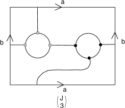
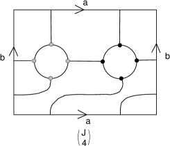
Figure 1:

The structure of this result is easy do understand combinatorically. We have to find the possible ways of connecting two necklaces with each, respectively, $J$ white ($Z$’s) and $J$ black ($\bar{Z}$’s) beads according to the following rules: (a) each connection has to link a black to a white bead (b) in order to find the ${\cal O}(N^{J-2h})$ contribution the connections have to be drawn without crossing on a genus $h$ surface such that no handle of the surface can be collapsed without pinching a connection. Let us call all connections that run (possibly after topological deformation) parallel to another connection “reducible”. Eliminate all reducible connections. This will lead to a number of inequivalent, irreducible graphs on the genus $h$ surface. These have $k$ connections ranging between at least $k=2h+1$ connections (easy to see) and at most $k=4h$ connections (harder to see). Even for a given number of irreducible connections there are (starting from genus $h=2$) an increasing number $a_{h,k}$ of inequivalent irreducible graphs. Once these numbers are worked out (this is a formidable problem, except for genus 1, where $k=3,4$ and there is only one irreducible graph in each case, see figure 1) the total number of graphs of irreduciblity type $k$ with $J$ connections is given by $a_{h,k}{J\choose k}$. This explains the above expansion eq.(2.8). We are now ready to investigate the large $J$ limit of the correlator; we see from eq.(2.8)

$$\langle{\rm Tr}Z^{J}~{}{\rm Tr}\bar{Z}^{J}\rangle=JN^{J}\Bigg{\{}1+\sum_{h=1}^{\infty}{a_{h,4h}\over(4h)!}{J^{4h}\over N^{2h}}+\ldots\Bigg{\}}$$ (2.9)

that the terms involving $a_{h,4h}$ stay finite in the double scaling limit $J,N\rightarrow\infty$ iff we keep ${J^{2}\over N}$ finite while all other terms in eq.(2.9) vanish. This means that non-planar diagrams survive to all orders in $1/N^{2}$. In addition the above analysis allows for the interpretation of the scaling limit eq.(1.1) already mentioned in the introduction: Clearly, in light of eq.(2.8), the omission of the subleading terms eliminates diagrams with “skinny” handles consisting of only a small number of string bits. The meaning of the double scaling limit is therefore that it combines a continuum limit (taking the size of lattice strings to infinity) with a large $N$ limit (ensuring that only “fat” handles are allowed). This is very similar to the matrix model double scaling limits discovered in [6]. One apparent difference is that in these “old” double scaling limits there is an exponential growth of the number of graphs at fixed genus. However, this exponential factor (which in our case would be a term like $c^{J}$) is well known to be non-universal, reestablishing the close similarity.

It is straightforward to explicitly find the scaling function from eq.(2.4)

$$G^{JJ^{\prime}}(x)=\frac{\delta^{JJ^{\prime}}}{|x|^{2J}}\left(\frac{g_{{\rm YM}}^{2}N}{8\pi^{2}}\right)^{J}\cdot J\cdot\frac{\sinh\left(\frac{1}{2}\frac{J^{2}}{N}\right)}{\frac{1}{2}\frac{J^{2}}{N}}$$ (2.10)

incidentally yielding the numbers $a_{h,4h}=(4h)!/((2h+1)!2^{2h})$.

At this point, one might raise the objection that the correct gauge group for the AdS/CFT correspondence is SU(N) rather than U(N) and the sub-leading orders in the large $N$ expansion differ for these two groups. Indeed, the analog of (2.4) can be found for SU(N),

$$\langle{\rm Tr}Z^{J}~{}{\rm Tr}\bar{Z}^{J}\rangle_{\rm SU(N)}=$$

$$J!N^{-J+2}(-1)^{J}+\sum_{p=1}^{J}\left(\matrix{J\cr p\cr}\right)^{2}\frac{(-1)^{J-p}(J-p)!N^{p-J}}{(p+1)}\left(\frac{\Gamma(N+p+1)}{\Gamma(N)}-\frac{\Gamma(N+1)}{\Gamma(N-p)}\right)$$

It can be seen that this formula has the same asymptotics in large $J$ as the previous case of U(N), though it has slower rate of convergence to the asymptote. From this, we conclude that the large $J$ limit of the U(N) and SU(N) gauge theories are similar enough that we can focus on U(N). Of course, this is true only for the scaling limit that we are considering. If, for example, $J$ goes to infinity faster than $N^{1/2}$, the limit could be more complicated.

Other two-point functions easily evaluated (for $U(N)$) are

$$\langle 0|{\rm Tr}\left(Z^{J}(x)\Phi^{3}(x)\right){\rm Tr}\left(\bar{Z}^{J^{\prime}}(0)\Phi^{3}(0)\right)|0\rangle=$$ (2.11)

$$\hskip 71.13188pt\,\left(\frac{g_{{\rm YM}}^{2}}{8\pi^{2}}\right)^{J+1}\frac{\delta^{JJ^{\prime}}}{|x|^{2J+2}}\left(\frac{\Gamma(N+J+2)}{\Gamma(N)}-\frac{\Gamma(N+1)}{\Gamma(N-J-1)}\right)$$

$$\hskip 71.13188pt\longrightarrow\,\frac{\delta^{JJ^{\prime}}}{|x|^{2J+2}}\left(\frac{g_{{\rm YM}}^{2}N}{8\pi^{2}}\right)^{J+1}\cdot\frac{\sinh\left(\frac{1}{2}\frac{J^{2}}{N}\right)}{\frac{1}{2}\frac{J^{2}}{N}}$$

and

$$\sum_{p=0}^{J}\langle 0|{\rm Tr}\left(Z^{J-p}(x)\Phi^{3}(x)Z^{p}(x)\Phi^{4}(x)\right){\rm Tr}\left(\bar{Z}^{J^{\prime}-q}(0)\Phi^{4}(0)\bar{Z}^{q}(0)\Phi^{3}(0)\right)|0\rangle=$$

$$\hskip 71.13188pt\frac{\delta^{JJ^{\prime}}}{|x|^{2J+4}}\left(\frac{g_{{\rm YM}}^{2}}{8\pi^{2}}\right)^{J+2}\left(\frac{\Gamma(N+J+2)}{\Gamma(N)}-\frac{\Gamma(N+1)}{\Gamma(N-J-1)}\right)$$ (2.12)

$$\hskip 71.13188pt\longrightarrow\frac{\delta^{JJ^{\prime}}}{|x|^{2J+4}}\left(\frac{g_{{\rm YM}}^{2}N}{8\pi^{2}}\right)^{J+2}\cdot\frac{\sinh\left(\frac{1}{2}\frac{J^{2}}{N}\right)}{\frac{1}{2}\frac{J^{2}}{N}}$$

The last of these is a correlator of a chiral primary field with a one which isn’t a chiral primary. This is due to the fact that the summation effectively symmetrizes the operator product. Since the sum depends on non-planar diagrams, the terms individually must also. This means that the quantity of interest,

$$\langle 0|{\rm Tr}\left(Z^{J-p}(x)\Phi^{3}(x)Z^{p}(x)\Phi^{4}(x)\right){\rm Tr}\left(\bar{Z}^{q}(0)\Phi^{4}(0)\bar{Z}^{J-q}(0)\Phi^{3}(0)\right)|0\rangle$$

must contain non-planar graphs in the limit (1.1). We shall discuss non-planar corrections to this correlator in section 4.

3 Three-point functions

It is interesting to consider the three-point function of chiral primary fields. In the AdS/CFT correspondence, such three-point functions should coincide with a 3-point amplitude for certain BPS states of the graviton. In the present case, we shall see that, like the case of the two-point correlator of chiral primary operators, the three-point function also obtains contributions from all genera in the limit (1.1).

Consider the three-point function of chiral primary operators

$$G^{JKL}(x,y) = \langle 0|{\rm Tr}\left(Z^{J}(x)\right){\rm Tr}\left(Z^{K}(y)\right){\rm Tr}\left(\bar{Z}^{L}(0)\right)|0\rangle$$ (3.1)

$$= \delta^{L-J-K,0}\left(\frac{g^{2}_{{\rm YM}}}{8\pi^{2}}\right)^{J+K}\frac{1}{|x|^{2J}|y|^{2K}}\,\langle{\rm Tr}Z^{J}{\rm Tr}Z^{K}{\rm Tr}\bar{Z}^{J+K}\rangle$$

with ($0<J,K,L<N$), where again the remaining expectation value can be evaluated using matrix model techniques (cf. appendix A)

$$\langle{\rm Tr}Z^{J}{\rm Tr}Z^{K}{\rm Tr}\bar{Z}^{J+K}\rangle = \frac{1}{J+K+1}\left\{\frac{\Gamma(N+J+K+1)}{\Gamma(N)}+\frac{\Gamma(N+1)}{\Gamma(N-J-K)}\right.$$ (3.2)

$$-\left.\frac{\Gamma(N+J+1)}{\Gamma(N-K)}-\frac{\Gamma(N+K+1)}{\Gamma(N-J)}\right\}$$

The scaling limit of the three-point function is

$$G^{JKL}(x,y) = 2\,\delta^{L-J-K,0}\,(J+K)\left(\frac{g^{2}_{{\rm YM}}N}{8\pi^{2}}\right)^{J+K}\frac{1}{|x|^{2J}|y|^{2K}}\,\cdot$$ (3.4)

$$\frac{\sinh\left(\frac{J(J+K)}{2N}\right)\sinh\left(\frac{K(J+K)}{2N}\right)}{\frac{(J+K)^{2}}{2N}}$$

We see that all genera contribute. Furthermore, the dependence of these functions on the parameters $J^{2}/N,K^{2}/N,L^{2}/N$ is one which cannot be removed by normalizing the operators. This implies a dependence of the three-point amplitude on the three parameters which are left over in the double-scaling limit.

4 Computing momentum correlators

We consider the following operators

$${\cal O}_{n}(x)=\frac{1}{\sqrt{J}\,N^{J/2+1}}\,\sum_{l=0}^{J}\mbox{Tr}[\,\phi_{3}\,Z^{l}\,\phi_{4}\,Z^{J-l}\,]\,e^{\frac{2\pi\,i\,n\,l}{J}}$$ (4.1)

Notice that these operators differ from those introduced in [3] by the inclusion of $l=0$ in the summation range. This difference will turn out to be important for what follows. We shall be interested in the two point correlator $\langle{\cal O}_{n_{1}}(x)\,\bar{\cal O}_{n_{2}}(0)\rangle$ up to next to leading order in $N^{2}$. In the free theory limit one has after contracting the $\phi_{3}$ and $\phi_{4}$’s

$$\langle\,{\cal O}_{n_{1}}(x)\,\bar{\cal O}_{n_{2}}(0)\,\rangle_{0-loop}=$$ (4.2)

$$\frac{1}{J\,N^{J+2}}\,\left(\frac{g_{{\rm YM}}^{2}}{8\pi^{2}|x|^{2}}\right)^{J+2}\sum_{p,q=0}^{J}\,\langle\,\mbox{Tr}[\,Z^{J-p}\,\bar{Z}^{J-q}\,]\,\mbox{Tr}[\,Z^{p}\,\bar{Z}^{q}\,]\,\rangle\,e^{\frac{2\pi\,i}{J}(n_{1}\,p-n_{2}\,q)}$$

The remaining correlator splits into a disconnected and connected piece

$$\langle\,\mbox{Tr}[\,Z^{J-p}\,\bar{Z}^{J-q}\,]\,\mbox{Tr}[\,Z^{p}\,\bar{Z}^{q}\,]\,\rangle=\delta_{p,q}\,[J\mid p]+[J\mid p,q\,]$$ (4.3)

where we have defined

$$[J\mid p\,] = \langle\mbox{Tr}[\,Z^{J-p}\,\bar{Z}^{J-p}\,]\,\rangle\,\langle\mbox{Tr}[\,Z^{p}\,\bar{Z}^{p}\,]\,\rangle$$

$$[J\mid p,q\,] = \langle\mbox{Tr}[\,Z^{J-p}\,\bar{Z}^{J-q}\,]\,\mbox{Tr}[\,Z^{p}\,\bar{Z}^{q}\,]\,\rangle_{conn}$$ (4.4)

The disconnected piece may easily be deduced from eq. (2.4) by making use of the identity

$$\langle{\rm Tr}(Z^{J+1}){\rm Tr}(\bar{Z}^{J+1})\rangle=(J+1)\langle{\rm Tr}(Z^{J}\bar{Z}^{J})\rangle$$ (4.5)

The result reads

$$[J\mid p]=N^{J+2}+N^{J}\,\Bigr{[}\left(\matrix{J-p+2\cr 4\cr}\right)+\left(\matrix{p+2\cr 4\cr}\right)\,\Bigl{]}\,+\,{\cal O}(N^{J-2})$$ (4.6)

The combinatorics of the connected contributions goes as follows. As the leading disconnected contribution to eq. (4.3) scales as $N^{J+2}$ we shall be interested only in the planar connected contribution to $[J\mid p,q\,]$. The relevant contractions are depicted in figure 2. Assume $J-q>p$ and $q>p$. Then we connect $k$ of the $(J-q)$ $\bar{Z}$’s with $k$ of the $p$ $Z$’s. There are $(p-k+1)\,(J-q-k+1)$ ways of doing this and we should sum over these $k$ contractions as $k=1,\ldots,p$. All the remaining contractions (depicted by dashed lines in the figure) are completely determined by planarity once the middle $k$ lines have been chosen. If we have no middle contractions ($k=0$) all the $p$ $Z$’s are contracted with $p$ $\bar{Z}$’s on the same ellipse, leaving $(q-p)$ $\bar{Z}$’s on the right ellipse of figure 2 to be contracted with the left ellipse. There are then $(q-p)\,(p+1)\,(J-q+1)$ ways of doing this. We hence see that

$$[J\mid p,q\,] = N^{J}\,\Bigl{[}\,\frac{1}{6}\,p\,(p+1)\,(3J+1-p-3q)$$ (4.7)

$$\qquad+(q-p)\,(p+1)\,(J-q+1)\,\Bigr{]}\,+\,{\cal O}(N^{J-2})$$

$$\mbox{for}\quad(q>p\,,\,J-q>p)$$

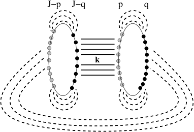
Figure 2: The contractions

For different regions of $p$ and $q$ the correlator is determined by the two obvious symmetries $(p\leftrightarrow q)$ and $(p\rightarrow J-p,q\rightarrow J-q)$ of $[J\mid p,q\,]$. One may now Fourier transform eq. (4.6) and eq. (4.7) and deduce the leading behaviours in $J^{2}/N$. For the disconnected contribution one finds

$$D_{n_{1}-n_{2}}=\sum_{p=0}^{J}\,[J\mid p\,]\,e^{\frac{2\pi\,i}{J}(n_{1}-n_{2})\,p}=$$

$$\qquad N^{J+2}\,(J+1)\,\delta_{n_{1},n_{2}}+$$ (4.8)

$$\qquad+N^{J}\,J^{5}\,\cases{\frac{1}{60}&$n_{1}=n_{2}$\cr\frac{8\pi^{2}n_{1}^{2}-3}{384n_{1}^{4}\pi^{4}}&$n_{1}=-n_{2}$\cr\frac{2\pi^{2}(n_{1}-n_{2})^{2}-3}{24(n_{1}-n_{2})^{4}\pi^{4}}&$n_{1}\neq n_{2}$\cr}\quad+N^{J}\,{\cal O}(J^{4})+{\cal O}(N^{J-2})$$

in the limit of large $J$. Let us now turn to the connected non-diagonal contribution to the correlator eq. (4.2). The summation domain for $p$ and $q$ then splits into four sectors $(q>p,J-q>p),(q>p,J-q<p),(q<p,J-q>p)$ and $(q<p,J-q<p)$ and due to the symmetries of $[J\mid p,q\,]$ the sum over these four sectors may be reduced to a single sum over the domain $(q>p,J-q>p)$ with varying phase factor contributions. Explicitly one has to evaluate the double sum

$$C_{n_{1},n_{2}}=2\,\sum_{p=0}^{[J/2]-1}\sum_{q=p+1}^{J-p-1}[J\mid p,q\,]\,\Bigl{(}\cos[{\textstyle\frac{2\pi}{J}}(p\,n_{1}-q\,n_{2})]+\cos[{\textstyle\frac{2\pi}{J}}(q\,n_{1}-p\,n_{2})]\,\Bigr{)}$$ (4.9)

where $[J/2]=J/2$ for $J$ even and $[J/2]=(J+1)/2$ for J odd. As $[J\mid p,q\,]$ scales as $p^{3}$ the double sum eq. (4.9) will scale as $J^{5}$ and its contribution is relevant to the momentum correlator in the double scaling limit. Performing the sums in eq. (4.9) and taking the $J\rightarrow\infty$ limit we find

$$C_{n_{1},n_{2}}=N^{J}\,J^{5}\,\cases{\frac{1}{40}&$n_{1}=n_{2}=0$\cr\frac{3-2\pi^{2}\,n^{2}}{24\,n^{4}\pi^{4}}&$n:=n_{1/2}\neq 0,n_{2/1}=0$\cr\frac{21-2\pi^{2}\,n^{2}}{48\,n^{4}\pi^{4}}&$n:=n_{1}=n_{2}$ and $n_{1}\neq 0\neq n_{2}$\cr\frac{9}{32n^{4}\pi^{4}}&$n:=n_{1}=-n_{2}$ and $n_{1}\neq 0\neq n_{2}$\cr\frac{2\,n_{1}{}^{2}-3\,n_{1}\,n_{2}+2\,n_{2}{}^{2}}{8\,n_{1}{}^{2}\,n_{2}{}^{2}\,(n_{1}-n_{2})^{2}\,\pi^{4}}&$n_{1}\neq n_{2}$ and $n_{1}\neq 0\neq n_{2}$\cr}$$ (4.10)

up to terms of order $N^{J}\,{\cal O}(J^{4})$ and ${\cal O}(N^{J-2})$. We now have to worry about the contributions along the “diagonals” $p=q$ and $J-q=p$ which were omitted in the double sum of eq. (4.9). The counting now works analogously, for the first case ($p=q$) one has

$$C^{p=q}_{n1-n2}=N^{J}\,\sum_{p=0}^{[J/2]}{\textstyle\frac{1}{6}}\,(p+1)\,p\,(3J+1-4p)\,2\,\cos[\,{\textstyle\frac{2\pi}{J}}\,(n_{1}-n_{2})p\,]$$ (4.11)

and for the second case ($J-q=p$) one finds

$$C^{J-q=p}_{n1-n2}=N^{J}\,\sum_{p=0}^{[J/2]}\,\Bigl{[}{\textstyle\frac{1}{6}}\,(p+1)\,p\,(2p+1)+(p+1)^{2}\,(J-2p)\,\Bigr{]}\,2\,\cos[\,{\textstyle\frac{2\pi}{J}}\,(n_{1}-n_{2})p\,]$$ (4.12)

These sums can be worked out explicitly, however, we already see at this point that they will not contribute at order $J^{5}$ as the summand scales as $p^{3}$. We hence have that

$$C^{p=q}_{n1-n2}\sim C^{J-q=p}_{n1-n2}\sim N^{J}\,{\cal O}(J^{4})$$ (4.13)

and these contributions are suppressed in the limit eq. (1.1). Summarizing we have thus found that

$$\langle\,{\cal O}_{n_{1}}(x)\,\bar{\cal O}_{n_{2}}(0)\,\rangle_{0-loop}=\left(\frac{g_{{\rm YM}}^{2}}{8\pi^{2}|x|^{2}}\right)^{J+2}\,\Bigr{[}\,\delta_{n_{1}n_{2}}+\frac{J^{4}}{N^{2}}\,M_{n_{1}n_{2}}+{\cal O}(\frac{J^{3}}{N^{2}})\,\Bigr{]}$$ (4.14)

where we have introduced the symmetric real matrix $M_{\bar{n}\bar{m}}$ given by

$$M_{00}=\frac{1}{24}\qquad M_{0\bar{n}}=0\qquad M_{\bar{n}\bar{m}}=\cases{\frac{2\pi^{2}(\bar{n}-\bar{m})^{2}-3}{24(\bar{n}-\bar{m})^{4}\pi^{4}}+\frac{2\,\bar{n}^{2}-3\,\bar{n}\,\bar{m}+2\,\bar{m}^{2}}{8\,\bar{n}^{2}\,\bar{m}^{2}\,(\bar{n}-\bar{m})^{2}\,\pi^{4}}&$|\bar{n}|\neq|\bar{m}|$\cr&\cr\frac{1}{60}+\frac{21-2\pi^{2}\,\bar{n}^{2}}{48\,\bar{n}^{4}\pi^{4}}&$\bar{n}=\bar{m}$\cr&\cr\frac{105+8\pi^{2}\bar{n}^{2}}{384\,\bar{n}^{4}\,\pi^{4}}&$\bar{n}=-\bar{m}$\cr}$$ (4.15)

Note the decoupling of the zero momentum sector ($M_{0\bar{n}}=0$) which corresponds to the groundstate not mixing under perturbation theory with the excited states in the dual string picture. This result tells us that we have to renormalize our momentum operators according to

$$\tilde{\cal O}_{n}(x)=\sum_{m}\Bigr{[}\,\delta_{nm}-\frac{J^{4}}{2\,N^{2}}\,M_{nm}\,\Bigr{]}\,{\cal O}_{m}(x)$$ (4.16)

in order to maintain orthogonality up to order $J^{4}/N^{2}$, i.e. $\langle\,\tilde{\cal O}_{n}\,\tilde{\cal O}_{m}\,\rangle\propto\delta_{n,m}$.

5 Computing anomalous dimensions

In this section we shall review the computation of anomalous dimensions of operators which are of interest to us in this paper. The correlation functions of interest are those of traces of products of the scalar fields, for example

$$\langle 0|:{\rm Tr}\Phi_{\alpha_{1}}(x)\ldots\Phi_{\alpha_{p}}(x)::{\rm Tr}\Phi_{\beta_{1}}(0)\ldots\Phi_{\beta_{q}}(0):|0\rangle=$$ (5.1)

$$\hskip 14.22636pt\delta_{pq}g_{{\rm YM}}^{2p}\Delta^{p}(x)\sum_{\rm Perm~{}P}\left(\delta_{\alpha_{1}\beta_{P(1)}}\ldots\delta_{\alpha_{p}\beta_{P(p)}}\right)+{\rm quantum~{}corrections}$$

Here, the dots $:...:$ indicate normal ordering, so that the vacuum expectation value of each individual operator vanishes. In the following, we will omit the normal ordering symbols. The first term on the right-hand-side is the correlator in the free field limit. The other terms, are given by radiative corrections to the free field limit. In this section, we will compute these radiative corrections to the next order in $g_{{\rm YM}}^{2}$.

5.1 Notation

The field content of ${\cal N}=4$ supersymmetric Yang-Mills theory in four dimensions are the scalars, $\Phi_{\alpha}(x)$ where the Greek indices $\alpha,\beta,\ldots=1,...,6$ transform under the R-symmetry SO(6)$\sim$SU(4), vectors $A_{\mu}(x)$ where $\mu=1,2,3,4$ is the space-time index and a sixteen component spinor $\Psi(x)$. These fields are Hermitean $N\times N$ matrices and for the most part in the following, the gauge group will be U(N). These fields can be expanded in terms of the generators $T^{a}$ of U(N) as

$$\Phi_{\alpha}(x)=\sum_{a=0}^{N^{2}-1}\phi^{a}_{\alpha}(x)T^{a}~{}~{},~{}~{}A_{\mu}(x)=\sum_{a=0}^{N^{2}-1}A_{\mu}^{a}(x)T^{a}~{}~{},~{}~{}\Psi(x)=\sum_{a=0}^{N^{2}-1}\psi^{a}(x)T^{a}$$ (5.2)

where $T^{0}_{kl}=\frac{1}{\sqrt{2N}}\delta_{kl}$ is the U(1) generator. We use the letters $a,b,\ldots=0,\ldots,N^{2}-1$ to denote components in the Lie algebra of U(N). The conventions for the generators and structure constants are

$$\left[T^{a},T^{b}\right]=if^{abc}T^{c}~{},~{}~{}{\rm Tr}(T^{a}T^{b})=\frac{1}{2}\delta^{ab}$$

Also,

$$\sum_{a=0}^{N^{2}-1}T^{a}_{ij}T^{a}_{kl}=\frac{1}{2}\delta_{il}\delta_{jk}~{},~{}~{}\sum_{a=1}^{N^{2}-1}T^{a}_{ij}T^{a}_{kl}=\frac{1}{2}\left(\delta_{il}\delta_{jk}-\frac{1}{N}\delta_{ij}\delta_{kl}\right)$$

and

$$f^{abc}f^{a^{\prime}bc}=N\delta^{aa^{\prime}}~{},~{}~{}f^{abc}f^{abc}=N(N^{2}-1)$$

We shall also need the identity

$$\mbox{Tr}(T^{a}\,A\,T^{b}\,B)\,\mbox{Tr}(T^{c}\,C\,T^{d}\,D)\,f^{ead}\,f^{ebc}=$$

$${\textstyle\frac{1}{8}}\Bigl{(}\mbox{Tr}\,A\,\mbox{Tr}\,C\,\mbox{Tr}\,BD+\mbox{Tr}\,B\,\mbox{Tr}\,D\,\mbox{Tr}\,AC-\mbox{Tr}\,ACBD\,-\mbox{Tr}\,ADBC\,\Bigr{)}$$

along with

$$\mbox{Tr}(T^{\bar{a}}\,A)\,\mbox{Tr}(T^{\bar{a}}\,B) = {\textstyle\frac{1}{2}}\,\mbox{Tr}\,AB-{\textstyle\frac{1}{2N}}\,\mbox{Tr}\,A\,\mbox{Tr}\,B$$

$$\mbox{Tr}(T^{\bar{a}}\,A\,T^{\bar{a}}\,B) = {\textstyle\frac{1}{2}}\,\mbox{Tr}\,A\,\mbox{Tr}\,B-{\textstyle\frac{1}{2N}}\,\mbox{Tr}\,AB$$ (5.4)

where $A,B,C,D$ are $N\times N$ matrices and $\bar{a}=1,\ldots,N^{2}-1$ runs only over the SU(N) indices. We use the conventions of [11, 12].

The Euclidean space action of ${\cal N}=4$ supersymmetric Yang-Mills theory is

$$S=\int d^{4}x\frac{1}{g^{2}_{{\rm YM}}}\left\{\frac{1}{4}F_{\mu\nu}^{a}F_{\mu\nu}^{a}+\frac{1}{2}(D_{\mu}\phi_{\alpha}^{a})^{2}+\frac{1}{4}\sum_{\alpha,\beta=1}^{6}f^{abc}f^{ade}\phi^{b}_{\alpha}\phi^{c}_{\beta}\phi^{d}_{\alpha}\phi^{e}_{\beta}+\right.$$

$$\left.+\frac{1}{2}\bar{\psi}^{a}\Gamma^{\mu}D_{\mu}\psi^{a}+\frac{1}{2}f^{abc}\bar{\psi}^{a}\Gamma^{\alpha}\phi^{b}_{\alpha}\psi^{c}\right\}$$ (5.5)

where the curvature is $F_{\mu\nu}^{a}=\partial_{\mu}A_{\nu}^{a}-\partial_{\nu}A_{\mu}^{a}+f^{abc}A_{\mu}^{b}A_{\nu}^{c}$ and the covariant derivative is $D_{\mu}\phi^{a}=\partial_{\mu}\phi^{a}+f^{abc}A^{b}_{\mu}\phi^{c}$. $(\Gamma^{\mu},\Gamma^{\alpha})$ are the ten-dimensional Dirac matrices in the Majorana-Weyl representation.

Vertices and propagators can be read off from the action (5.5). We will work in the Feynman gauge where the free field limit of the vector field propagator is

$$\langle 0|A^{a}_{\mu}(x)A_{\nu}^{b}(0)|0\rangle_{0}=g_{{\rm YM}}^{2}\delta^{ab}\delta_{\mu\nu}\frac{1}{4\pi^{2}[x]^{2}}$$

In this gauge, it resembles the free scalar field propagator

$$\langle 0|\phi^{a}_{\alpha}(x)\phi^{b}_{\beta}(0)|0\rangle_{0}=g_{{\rm YM}}^{2}\delta^{ab}\delta_{\alpha\beta}\frac{1}{4\pi^{2}[x]^{2}}$$

${\cal N}=4$ supersymmetric Yang-Mills theory contains no dimensional parameters. Furthermore, because of the high degree of supersymmetry, it has vanishing beta function for the coupling constant $g_{{\rm YM}}$ and is a conformal field theory. However, individual Feynman diagrams are divergent and the explicit computations that we do in the following will require a regularization. For this purpose, we will use regularization by dimensional reduction. Four dimensional ${\cal N}=4$ supersymmetric Yang-Mills theory is a dimensional reduction of the ten-dimensional ${\cal N}=1$ theory. We can obtain a regularization of the four dimensional theory which still has sixteen supersymmetries (but of course is no longer conformally invariant) by considering a dimensional reduction to $2\omega$ dimensions, rather than 4 dimensions. In this reduction, the fermion content is still a sixteen-component spinor (which originally was the Weyl-Majorana spinor in ten dimensions). There are $10-2\omega$ rather than $6$ flavors of scalar field and $2\omega$ rather than $4$ polarizations of the vector field.

The Green function for the Laplacian in $2\omega$ dimensions is

$$\Delta(x)=\int\frac{d^{2\omega}p}{(2\pi)^{2\omega}}\frac{e^{ip\cdot x}}{p^{2}}=\frac{\Gamma(\omega-1)}{4\pi^{\omega}[x^{2}]^{\omega-1}}$$ (5.6)

When we work in $2\omega$-dimensions, the right-hand side of this equation should replace $1/4\pi^{2}[x^{2}]$ in propagators. Useful formulae for Feynman integrals in $2\omega$-dimensions can be found in refs.[11, 12].

5.2 One-loop integrals

The Feynman diagrams which contribute to radiative corrections to two-point correlators of scalar trace operators are depicted in figure 3. The first diagram in figure 3 contains the self-energy of the scalar field. Feynman rules and conventions for vertices can be deduced from the action (5.5).

The self-energy of the scalar field was computed with the present notational conventions in refs.[11, 12]. Written as a correction to the scalar propagator, it is

$$\langle 0|\phi^{a}_{\alpha}(x)\phi^{b}_{\beta}(0)|0\rangle=$$ (5.7)

$$\hskip 14.22636ptg_{{\rm YM}}^{2}\delta_{\alpha\beta}\Delta(x)\left(\delta^{ab}+\delta^{\bar{a}\bar{b}}\left[-\frac{g_{{\rm YM}}^{2}N\Gamma(\omega-1)}{8\pi^{\omega}(2-\omega)(2\omega-3)}\right][x^{2}]^{(2-\omega)}+\ldots\right)$$

Note that the quantum correction only affects the SU(N) indices. The $\ldots$ denote terms of order at least $g_{{\rm YM}}^{6}$.

Figure 3: The relevant graphs of the self energy, gluon exchange and four-point interaction contributing to the leading radiative corrections of two-point scalar field trace operators.

The other quantum correction that we must take into account occurs in the correlator of four scalar fields,

$$\Gamma^{abcd}_{\alpha\beta\gamma\delta}(x) \equiv \langle 0|\phi^{a}_{\alpha}(x)\phi^{b}_{\beta}(x)\phi^{c}_{\gamma}(0)\phi^{d}_{\delta}(0)|0\rangle$$ (5.8)

$$= g_{{\rm YM}}^{4}\Delta^{2}(x)~{}\left(\delta^{ac}\delta^{bd}\delta_{\alpha\gamma}\delta_{\beta\delta}+\delta^{ad}\delta^{bc}\delta_{\alpha\delta}\delta_{\beta\gamma}\right)+\delta\Gamma^{abcd}_{\alpha\beta\gamma\delta}(x)$$

The first term on the right-hand-side is the free field limit and $\delta\Gamma^{abcd}_{\alpha\beta\gamma\delta}(x)$ denotes the radiative corrections, which we shall compute to order $g_{{\rm YM}}^{6}$. The relevant Feynman diagrams are the second and third diagrams in figure 3. When these diagrams are combined, the total contribution is conveniently summarized in a combination of three different tensor structures,

$$\delta\Gamma^{abcd}_{\alpha\beta\gamma\delta}(x)=g^{6}_{\rm YM}\times$$ (5.9)

$$\Big{[}\left(\delta_{\alpha\gamma}\delta_{\beta\delta}f^{\small eac}f^{\small ebd}+\delta_{\alpha\delta}\delta_{\beta\gamma}f^{\small ead}f^{\small ebc}\right)\left[\frac{\Gamma(\omega-1)}{4\pi^{\omega}(2-\omega)(2\omega-3)}\right][x^{2}]^{2-\omega}\Delta^{2}(x)+$$

$$\left(\delta_{\alpha\delta}\delta_{\beta\gamma}-\delta_{\alpha\gamma}\delta_{\beta\delta}\right)f^{\small eab}f^{\small ecd}\left[\frac{\Gamma^{2}(\omega-2)\Gamma^{2}(\omega-1)\Gamma(3\omega-4)}{16\pi^{\omega}\Gamma^{2}(2\omega-2)\Gamma(4-2\omega)}\right][x^{2}]^{2-\omega}\Delta^{2}(x)+$$ (5.10)

$$\delta_{\alpha\beta}\delta_{\gamma\delta}\left(f^{\small eda}f^{\small ecb}+f^{\small edb}f^{\small eca}\right)\left[\frac{\Gamma^{2}(\omega-2)\Gamma^{2}(\omega-1)\Gamma(3\omega-4)}{16\pi^{\omega}\Gamma^{2}(2\omega-2)\Gamma(4-2\omega)}\right][x^{2}]^{2-\omega}\Delta^{2}(x)\Big{]}$$ (5.11)

Here, we have dropped a possible contact term which, in four dimensions, is proportional to the Dirac delta function $\delta(x)$ and therefore cannot contribute. The terms are arranged so that the first part (5.9) is symmetric, the second term (5.10) is anti-symmetric and the third term (5.11) is diagonal in the indices $\alpha$ and $\beta$. We caution the reader that the symmetric term (5.9) is not traceless. However, it is the only one which will be needed when we compute the leading radiative corrections to a correlator of chiral primary operators.

5.3 Cancellation of leading radiative corrections to 2-point correlator of chiral primary operators

The cancellation of leading order corrections to two- and three-point functions of chiral primary operators was demonstrated in ref.[13]. Here, to check our own procedure, and further develop the matrix model approach to computations we will redo this check of the no-renormalization theorem.

We will consider the two-point correlator of chiral primary operators,

$$\langle 0|{\rm Tr}Z^{J}(x)~{}{\rm Tr}\bar{Z}^{J}(0)|0\rangle=\frac{\Delta^{J}(x)}{2^{J}}\cdot\langle{\rm Tr}Z^{J}~{}{\rm Tr}\bar{Z}^{J}\rangle+\ldots$$ (5.12)

The first term on the right-hand-side is the free field limit which is given by the Feynman diagram depicted in figure 4. The last bracket in this term is the matrix model correlation function in eqn.(2.3). The factor $\Delta^{J}(x)$ is the $J^{\prime}$th power of the scalar correlation function and the combinatorics of taking traces of Lie algebra generators in the appropriate permutations is solved by the matrix model correlator, which we have evaluated explicitly in eqn.(2.4).

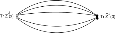
Figure 4: Feynman diagram for the free field limit of the correlator $\langle 0|{\rm Tr}Z^{J}(x)\,{\rm Tr}\bar{Z}^{J}(0)|0\rangle$. There are $J$ scalar propagators connecting the points $x$ and $0$.

Radiative corrections to this result arise from the Feynman diagrams, typical ones of which are depicted in figure 5. The first of the diagrams represent the radiative correction coming from the self-energy of the scalar field. As we discussed in the previous subsection, this gives a contribution consisting of a factor of the scalar self-energy times the number of scalar lines in the diagram. Thus, the correction from self-energies is

$$\left[-\frac{g^{2}_{{\rm YM}}N\Gamma(\omega-1)}{8\pi^{\omega}(2-\omega)(2\omega-3)}\right]\cdot[x^{2}]^{(2-\omega)}2^{-J}\Delta^{J}(x)\cdot J^{2}\langle{\rm Tr}T^{\bar{a}}Z^{J-1}~{}{\rm Tr}T^{\bar{a}}Z^{J-1}\rangle$$

where we have taken into account that the interaction affects only the SU(N) part of the propagator by inserting the SU(N) generators $T^{\bar{a}}$ into the traces and eliminating one factor of $Z$ and $\bar{Z}$ from each trace, respectively. The factor of $J^{2}$ reflects the fact that there are $J$ positions at which $T^{\bar{a}}$ could be inserted in each product. This equation can be simplified using (5.4) to get

$$\left[-\frac{g^{2}_{{\rm YM}}N\Gamma(\omega-1)}{8\pi^{\omega}(2-\omega)(2\omega-3)}\right]\cdot[x^{2}]^{(2-\omega)}2^{-J}\Delta^{J}(x)\frac{J^{2}}{2}\langle{\rm Tr}Z^{J-1}\bar{Z}^{J-1}-\frac{1}{N}{\rm Tr}Z^{J-1}{\rm Tr}\bar{Z}^{J-1}\rangle$$ (5.13)

  

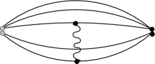
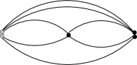
Figure 5: Feynman diagrams contributing to the order $g^{2}_{{\rm YM}}$ corrections to the correlator $\langle 0|{\rm Tr}Z^{J}(x)\,{\rm Tr}\bar{Z}^{J}(0)|0\rangle$. There are either $J$ scalar lines with one insertion of a scalar self-energy sub-diagram or two lines connected by either a vector line with two three-point vertices or one four-point scalar vertex.

The second and third of these diagrams represents the correction which correlates four of the scalar fields. This is the object $\Gamma$ which we studied in the previous section in eqs.(5.8)-(5.11). To take this correction into account, we must insert the four-point module $\Gamma$ in all appropriate ways. The result is given by the formula

$$\frac{J^{2}}{4}\sum_{k,q=0}^{J-2}\langle 0|{\rm Tr}\left(T^{a}Z^{k}(x)T^{b}Z^{J-2-k}(x)\right){\rm Tr}\left(T^{c}\bar{Z}^{q}(0)T^{d}\bar{Z}^{J-2-q}(0)\right)|0\rangle\Gamma_{zz\bar{z}\bar{z}}^{abcd}(x)$$

The factor of $J^{2}$ in the above expression arises from the fact that there are $J$ places to insert the first leg of $\Gamma$ into each of the two traces in the correlator. The position of the second insertion on each side is then summed over. The factor of 4 in the denominator arises from the fact that all crossings have already been taken into account in $\Gamma$ so that, to prevent double counting, the insertions should be ordered. It is more convenient to use the cyclic symmetry of the trace to consider all orderings and divide by their number - thus the factor of 4. Using the identity in (5.1), and the explicit form of the four-point module in eqn.(5.9), we get the formula

$$\frac{J^{2}}{8}\left[\frac{g^{2}_{{\rm YM}}\Gamma(\omega-1)}{4\pi^{\omega}(2-\omega)(2\omega-3)}\right][x^{2}]^{2-\omega}2^{-J}\Delta^{J}(x)~{}~{}~{}~{}~{}~{}~{}~{}~{}~{}$$

$$~{}~{}~{}~{}~{}~{}~{}\times~{}~{}\sum_{k,q=0}^{J-2}\langle{\rm Tr}Z^{k}{\rm Tr}\bar{Z}^{q}{\rm Tr}Z^{J-2-k}\bar{Z}^{J-2-q}-{\rm Tr}Z^{k}\bar{Z}^{q}Z^{J-2-k}\bar{Z}^{J-2-q}\rangle$$ (5.14)

In order to show that the radiative corrections cancel to order $g_{{\rm YM}}^{2}$, we must demonstrate that the sum of the two contributions, (5.13) and (5.14) is zero. This requires an identity for the matrix model correlation functions

$$\langle{\rm Tr}Z^{J-1}\bar{Z}^{J-1}-\frac{1}{N}{\rm Tr}Z^{J-1}{\rm Tr}\bar{Z}^{J-1}\rangle=$$ (5.16)

$$\frac{1}{N}\sum_{k,q=0}^{J-2}\langle{\rm Tr}Z^{k}{\rm Tr}\bar{Z}^{q}{\rm Tr}Z^{J-2-k}\bar{Z}^{J-2-q}-{\rm Tr}Z^{k}\bar{Z}^{q}Z^{J-2-k}\bar{Z}^{J-2-q}\rangle$$

This identity can easily be shown to follow from a Schwinger-Dyson equation of the Gaussian matrix model. Showing that it is true is entirely equivalent to the manipulations of Lie algebra matrices which was outlined in section 2 of ref.[13].

5.4 The first radiative correction to the anomalous dimension of unprotected operators to leading order in $\frac{J^{2}}{N}$

Here we shall be interested in calculating the first radiative correction to the anomalous dimension of the unprotected operators given in (4.1). Our calculation implies evaluating the first radiative correction to the following quantity

$$\sum_{p,q=0}^{J}\langle{\rm Tr}\left[\phi_{3}(x)Z^{J-p}(x)\phi_{4}(x)Z^{p}(x)\right]{\rm Tr}\left[\phi_{3}(0)\bar{Z}^{q}(0)\phi_{4}(0)\bar{Z}^{J-q}(0)\right]\rangle e^{\frac{2\pi i}{J}(n_{1}p-n_{2}q)}$$

The calculation is conveniently split into four parts each of which is treated making use of our modules from before

1. Corrections coming from self-energies, $C_{SE}$

   These result from replacing one free propagator of type $\langle\phi\phi\rangle$ or $\langle ZZ\rangle$ by the relevant one of the following two modules

   $$\langle 0|Z^{a}(x)\bar{Z}^{b}(0)|0\rangle = -\delta_{ab}\,\,\frac{g^{2}_{{\rm YM}}N}{8\pi^{2}(2-\omega)}\Delta(x)$$

   $$\langle 0|\phi_{\alpha}^{a}(x)\phi_{\beta}^{b}(0)|0\rangle = -\delta_{ab}\,\delta_{\alpha\beta}\,\frac{g^{2}_{{\rm YM}}N}{8\pi^{2}(2-\omega)}\Delta(x)$$

2. Corrections involving the correlator of four $Z$ fields, $C_{4Z}$

   These are obtained by replacing a pair of $Z$-propagators with the following module which can easily be derived from the general correlator (5.9)–(5.11)

   $$\langle 0|Z^{a}(x)Z^{b}(x)\bar{Z}^{c}(0)\bar{Z}^{d}(0)|0\rangle=\frac{g^{2}_{{\rm YM}}}{4\pi^{2}(2-\omega)}\left[f^{ead}f^{ebc}+f^{eac}f^{ebd}\right]\left(\Delta(x)\right)^{2}$$ (5.17)

3. Corrections involving the correlator of four $\phi$-fields, $C_{4\phi}$

   These we get by replacing the two $\phi$-propagators with the following quantity

   $$\langle 0|\phi_{3}^{a}(x)\phi_{4}^{b}(x)\phi_{3}^{c}(0)\phi_{4}^{d}(0)|0\rangle=\frac{g^{2}_{{\rm YM}}}{4\pi^{2}(2-\omega)}\left[f^{ead}f^{ebc}\right]\left(\Delta(x)\right)^{2}$$ (5.18)

4. Corrections involving the correlator of two $Z$-fields and two $\phi$-fields, $C_{2Z\phi}$

   These are obtained by replacing one $Z$-propagator and one $\phi$-propagator with the following module

   $$\langle 0|\phi_{3}^{a}(x)Z^{b}(x)\phi_{3}^{c}(0)\bar{Z}^{d}(0)|0\rangle=\frac{g^{2}_{{\rm YM}}}{4\pi^{2}(2-\omega)}\left[f^{ead}f^{ebc}\right]\left(\Delta(x)\right)^{2}$$ (5.19)

Inserting the given modules in all possible ways and taking care of the remaining contractions by use of the trace formulas in section 5.1 we obtain to the leading order in $N$ and all orders in $J$

$$C^{0}_{SE} = A_{0}\cdot\cases{-\frac{J}{2}-1&$n_{1}\neq n_{2}$\cr-\frac{J^{2}}{2}-\frac{3J}{2}-1&$n_{1}=n_{2}$\cr}$$

$$C^{0}_{4Z} = A_{0}\cdot\cases{\frac{J}{2}&~{}~{}~{}~{}~{}~{}~{}~{} $n_{1}\neq n_{2}$\cr\frac{J^{2}}{2}-\frac{J}{2}&$~{}~{}~{}~{}~{}~{}~{}~{}~{}n_{1}=n_{2}$\cr}$$

$$C^{0}_{4\phi} = A_{0}\cdot\cases{1&~{}~{}~{}~{}~{}~{}~{}~{}~{}~{}~{}~{}~{}~{}~{} $n_{1}\neq n_{2}$\cr 1&~{}~{}~{}~{}~{}~{}~{}~{}~{}~{}~{}~{}~{}~{}~{}~{}$n_{1}=n_{2}$\cr}$$

$$C^{0}_{2\phi Z} = A_{0}\cdot\cases{0&~{}$n_{1}\neq n_{2}$\cr 2J\cos\left(\frac{2\pi n_{2}}{J}\right)&~{}$n_{1}=n_{2}$\cr}$$

where

$$A_{0}=\frac{g_{{\rm YM}}^{2}N}{4\pi^{2}(2-\omega)}\ \left(\frac{1}{2}\right)^{J+2}N^{J+2}\left[x^{2}\right]^{2-\omega}\Delta^{J+2}(x)$$ (5.20)

It is easy to understand the combinatorial factors of $(J+2)$ and $(J+1)(J+2)$ occurring in the self-energy correction. The factor $(J+2)$ counts the number of propagators and the $(J+1)$ the number of momentum states. The results neatly sum up to

$$C \equiv C_{SE}+C_{4Z}+C_{4\phi}+C_{2Z\phi}$$

$$= \cases{0&$n_{1}\neq n_{2}$\cr A_{0}\cdot 2J\left(\cos\left(\frac{2\pi n_{2}}{J}\right)-1\right)&$n_{1}=n_{2}$\cr}$$

The contribution to the correction of the anomalous dimension coming from planar diagrams thus reads

$$\left(\delta\Delta\right)_{0}=\frac{g_{{\rm YM}}^{2}Nn^{2}}{J^{2}}$$ (5.21)

which is the same as the result obtained in reference [3]. We note, however, that it is crucial for the cancellations to take place that we include $p,q=0$ in our summation range (5.4).

5.5 The first radiative correction to the anomalous dimension of unprotected operators to two orders in $\frac{J^{2}}{N}$

Calculation of the first radiative correction to the anomalous dimension can be carried out to higher orders in the double scaling parameter following exactly the same recipe as in the previous section. For the explicit computations it is useful to employ an effective matrix model interaction vertex representing the four point modules of eq. (5.17), eq. (5.18) and eq. (5.19). These computations are rather technical and we have chosen to present them in detail in appendix B.

The outcome of this analysis is that up to next to leading order in $N$ the correlation function in question at one-loop reads

$$\langle\,{\cal O}_{n_{1}}(x)\,\bar{\cal O}_{n_{2}}(0)\,\rangle_{\mbox{\tiny 1-loop}}=$$

$$-\frac{g^{2}_{{\rm YM}}\,N}{J^{2}}\,\frac{[x^{2}]^{2-\omega}}{4\pi^{2}\,(2-\omega)}\,\left(\frac{g^{2}_{{\rm YM}}}{8\pi^{2}\,|x|^{2}}\right)^{J+2}\,\Bigg{[}\,2\,n_{1}\,n_{2}\,(2\pi)^{2}\,\langle{\cal O}_{n_{1}}\,\bar{\cal O}_{n_{2}}\rangle_{\mbox{\tiny 0-loop}}+\frac{J^{4}}{N^{2}}\,{\cal D}_{n_{1},n_{2}}\,\Bigg{]}$$

where

$$\langle{\cal O}_{n_{1}}\,\bar{\cal O}_{n_{2}}\rangle_{\mbox{\tiny 0-loop}}=\delta_{n_{1},n_{2}}+\frac{J^{4}}{N^{2}}\,M_{n_{1},n_{2}}$$ (5.23)

is the tree-level correlator of eq. (4.14) and where ${\cal D}_{n_{1},n_{2}}$ is the symmetric genus one mass renormalization matrix given by ($\bar{n}\neq 0$)

$${\cal D}_{0,0}=0\qquad{\cal D}_{0,\bar{n}}=0\qquad{\cal D}_{\bar{n}_{1},\bar{n}_{2}}=\cases{\frac{2}{3}+\frac{5}{\bar{n}_{1}{}^{2}\,\pi^{2}}&for $|\bar{n}_{1}|=|\bar{n}_{2}|$\cr\frac{2}{3}+\frac{2}{\bar{n}_{1}{}^{2}\,\pi^{2}}+\frac{2}{\bar{n}_{2}{}^{2}\,\pi^{2}}&for $|\bar{n}_{1}|\neq|\bar{n}_{2}|$}$$ (5.24)

This result teaches us that for the redefined operators $\tilde{\cal O}_{n}(x)$ of eq. (4.16) we have

$$\langle\,\tilde{\cal O})_{n_{1}}(x)\,\tilde{\bar{\cal O}}_{n_{2}}(0)\,\rangle_{\mbox{\tiny 1-loop}}=-\frac{g^{2}_{{\rm YM}}\,N}{J^{2}}\,\frac{[x^{2}]^{2-\omega}}{4\pi^{2}\,(2-\omega)}\,\left(\frac{g^{2}_{{\rm YM}}}{8\pi^{2}\,|x|^{2}}\right)^{J+2}\,$$

$$\Bigl{[}\,2\,n_{1}\,n_{2}\,(2\pi)^{2}\,\delta_{n_{1},n_{2}}-(n_{1}-n_{2})^{2}\,(2\pi)^{2}\,\frac{J^{4}}{N^{2}}\,M_{n_{1},n_{2}}+\frac{J^{4}}{N^{2}}\,{\cal D}_{n_{1},n_{2}}\,\Bigr{]}$$

The diagonal piece of this result gives rise to a non-planar correction of the one-loop anomalous dimension of these operators

$$(\delta\Delta)_{1}=g^{2}_{{\rm YM}}\,\frac{J^{2}}{(2\pi)^{2}\,N^{2}}\,\Bigl{[}\,\frac{1}{3}+\frac{5}{2\,\bar{n}{}^{2}\,\pi^{2}}\,\Bigr{]}\,.$$ (5.26)

It would be very interesting to reproduce this result from a genus one string theory calculation.

Acknowledgments

We would like to thank Gleb Arutyunov and Niklas Beisert for interesting discussions. J.P. and M.S. would like to thank the University of British Columbia for hospitality during the initial stages of this project.

Appendix A Complex matrix model technology

Much of our insight into the nature of the scaling limit eq.(1.1) comes from the exact result eq.(2.4) which we have not been able to find in the literature. Here we will explain its derivation using matrix model techniques.

We start from the normalized Gaussian measure for complex $N\times N$ matrices $Z_{i,j}=$Re$Z_{i,j}+i~{}$Im$Z_{i,j}$ with $\bar{Z}_{i,j}=$Re$Z_{j,i}-i~{}$Im$Z_{j,i}$

$$\big{[}dZd\bar{Z}\big{]}=dZd\bar{Z}~{}\exp(-{\rm Tr}Z\bar{Z}),$$ (A.1)

where the flat measure $dZd\bar{Z}$ is an abbreviation of

$$dZd\bar{Z}=\prod_{i,j=1}^{N}{d{\rm Re}Z_{i,j}~{}d{\rm Im}Z_{i,j}\over\pi}$$ (A.2)

Thus $\int\big{[}dZd\bar{Z}\big{]}=1$, and matrix model expectation values are given by $\langle\ldots\rangle=\int\big{[}dZd\bar{Z}\big{]}\ldots$. The model has a $U(N)\times U(N)$ symmetry (since the action and the measure are invariant under independent left and right group multiplication $Z\rightarrow UZV^{\dagger}$ where $U,V$ are unitary). Correlators invariant under the full symmetry (i.e. sums of products of traces of powers of $Z\bar{Z}$) are calculable with known techniques [8]. Correlators with less symmetry are more difficult even though the potential is Gaussian. For our purposes we are interested in correlators invariant under the adjoint action of just one $U(N)$ symmetry: $Z\rightarrow UZU^{\dagger}$. Now the general invariant correlator contains traces of arbitrary words made out of $Z$ and $\bar{Z}$, a problem that has not been solved to our knowledge. However, in the special case where the traces contain either just $Z$’s or $\bar{Z}$’s the problem is solvable by character expansion techniques [9], or, alternatively, by the method of Ginibre [10]. For completeness we will briefly explain both.

In order to apply the first method one expands the parts of the correlator containing the $Z$’s and the $\bar{Z}$’s separately in the basis of unitary group characters (Schur functions) $\chi_{h}(Z)$ and $\chi_{h^{\prime}}(\bar{Z})$ labeled by Young diagrams $h$,$h^{\prime}$. Then one uses [9] that, even though the matrices are complex instead of unitary, the inner product

$$\langle\chi_{h}(Z)~{}\chi_{h^{\prime}}(\bar{Z})\rangle=\delta_{h,h^{\prime}}~{}\Omega_{h}$$ (A.3)

is still orthogonal, with a Young diagram dependent, explicitly known normalization factor $\Omega_{h}$ (see [9] for precise definitions). By Schur-Weyl duality the expansion coefficients are expressed with the help of the characters of the symmetric group $S_{N}$. E.g. in the simplest case $\langle{\rm Tr}Z^{J}~{}{\rm Tr}\bar{Z}^{J}\rangle$ one has

$${\rm Tr}Z^{J}=\sum_{h}{\rm ch}_{h}(J)~{}\chi_{h}(Z)$$ (A.4)

where ch${}_{h}(J)$ is the character of the symmetric group $S_{J}$ corresponding to the representation $h$ and evaluated for the conjugacy class of $J$-cycles. Thus, using eq.(A.3),

$$\langle{\rm Tr}Z^{J}~{}{\rm Tr}\bar{Z}^{J}\rangle=\sum_{h}\Big{(}{\rm ch}_{h}(J)\Big{)}^{2}~{}\Omega_{h}$$ (A.5)

Now it is easy to show that for $J-$cycles ch${}_{h}(J)$ is non-zero only for Young diagrams consisting of a single hook of boxes with row length $k$ and column length $J-k$. For the hooks one has ch${}_{h}(J)=\pm 1$ and (see [9]) $\Omega_{h}=\prod_{i=1}^{k}(N-1+i)~{}\prod_{m=1}^{J-k}(N-m)$ and thus (clearly $\sum_{h}$ becomes a sum over the $J$ possible hooks)

$$\langle{\rm Tr}Z^{J}~{}{\rm Tr}\bar{Z}^{J}\rangle=\sum_{k=1}^{J}~{}\prod_{i=1}^{k}(N-1+i)~{}\prod_{m=1}^{J-k}(N-m)$$ (A.6)

which may be summed to the expression eq.(2.4). In a similar way we find

$$\langle{\rm Tr}Z^{J}{\rm Tr}Z^{K}{\rm Tr}\bar{Z}^{J+K}\rangle=\Bigg{(}\sum_{k=K+1}^{J+K}-\sum_{k=1}^{J}\Bigg{)}~{}\prod_{i=1}^{k}(N-1+i)~{}\prod_{m=1}^{J+K-k}(N-m)$$ (A.7)

which upon summing gives eq.(3.2).

An alternative method consists in diagonalizing $Z$ by a similarity transformation

$$XZX^{-1}=\mbox{diag}(z_{1},\ldots,z_{N}),$$ (A.8)

with $X$ a complex matrix and $z_{1},\ldots,z_{N}$ the complex eigenvalues of $Z$. As shown by Ginibre in 1965 [10] the non-diagonal degrees of freedom can be integrated out leading to the following joint probability density for the eigenvalues of $Z$

$$P(z_{1},\ldots,z_{N})=K^{-1}\exp\left(-\sum_{i=1}^{N}|z_{i}|^{2}\right)\prod_{1\leq i\leq j\leq N}|z_{i}-z_{j}|^{2},\hskip 14.22636ptK=\pi^{N}\prod_{j=1}^{N}j!$$ (A.9)

Here the normalization is such that

$$\int_{C|}\,\prod_{i=1}^{N}d^{\,2}z_{i}\,P(z_{1},\ldots,z_{N})=1.$$ (A.10)

Furthermore, one can derive an explicit expression for the correlation function involving $n$ eigenvalues, defined as follows $(n<N)$

$$R_{n}(z_{1},\ldots,z_{n})\equiv\int_{C|}\,\prod_{i=n+1}^{N}d^{\,2}z_{i}\,P(z_{1},\ldots,z_{N}).$$ (A.11)

The result reads [10]

$$R_{n}(z_{1},\ldots,z_{n})=\pi^{-n}\,\frac{(N-n)!}{N!}\exp\left(-\sum_{k=1}^{n}|z_{k}|^{2}\right){\mbox{det}}(K_{N}(z_{i},z_{j}))|_{i,j=1,\ldots,n}$$ (A.12)

where

$$K_{N}(z_{i},z_{j})=\sum_{l=0}^{N-1}\frac{(z_{i}z_{j}^{*})^{l}}{l!}.$$ (A.13)

Making use of the expression (A.12) for $n=1$, $n=2$ and $n=3$ one easily derives (2.4) and (3.2).

Appendix B Evaluating $C_{4Z}$,$C_{2\phi Z}$,$C_{4\phi}$ and $C_{SE}$

B.1 $C_{4Z}$

Let us begin with the computation of $C_{4Z}$, i.e. the insertion of the module eq. (5.17) into the correlator. Here it is useful to represent the expression eq. (5.17) through an effective four point vertex in the matrix model of the form $:\mbox{Tr}(Z^{2}\bar{Z}^{2}-Z\bar{Z}Z\bar{Z}):$. This effective vertex appears in a normal ordered fashion, disallowing self-contractions. After performing the $\phi_{3}$ and $\phi_{4}$ contractions one is then led to evaluate the correlator

$$\langle\mbox{Tr}Z^{J-p}\,\bar{Z}^{J-q}\,\mbox{Tr}Z^{p}\,\bar{Z}^{q}\,:\mbox{Tr}(Z^{2}\bar{Z}^{2}-Z\bar{Z}Z\bar{Z}):\rangle$$

Contacting the two $Z$’s in the effective vertex with the outside $\bar{Z}$’s one produces, after some manipulations, the following three terms

$$(A) = \sum_{l=0}^{q-1}\,\sum_{m=0}^{J-q-1}\,\langle\mbox{Tr}(Z^{J-p}\,\bar{Z}^{m+q+1-l}\,Z^{p}\,\bar{Z}^{J+l-q-1-m})$$

$$\qquad\qquad-\mbox{Tr}(Z^{J-p}\,\bar{Z}^{m+q-l}\,Z^{p}\,\bar{Z}^{J+l-q-m})\rangle$$

$$(B) = \sum_{l=1}^{q-1}\,\sum_{m=0}^{l-1}\,\langle\mbox{Tr}(Z^{J-p}\,\bar{Z}^{J-q})\,\Bigl{(}\mbox{Tr}\bar{Z}^{m}\,\mbox{Tr}(Z^{p}\,\bar{Z}^{q-m})-\mbox{Tr}\bar{Z}^{m+1}\,\mbox{Tr}(Z^{p}\,\bar{Z}^{q-m-1})\,\Bigr{)}\rangle$$

$$(C) = \sum_{l=0}^{q-2}\,\sum_{m=0}^{q-l-2}\,\langle\mbox{Tr}(Z^{J-p}\,\bar{Z}^{J-q})\,\Bigl{(}\mbox{Tr}\bar{Z}^{m+2}\,\mbox{Tr}(Z^{p}\,\bar{Z}^{q-m-2})$$

$$\qquad\qquad-\mbox{Tr}\bar{Z}^{m+1}\,\mbox{Tr}(Z^{p}\,\bar{Z}^{q-m-1})\,\Bigr{)}\rangle$$

to be augmented by the corresponding terms obtained by swapping $p\rightarrow J-p$ and $q\rightarrow J-q$. We are interested in these correlators to orders $N^{J+3}$ and $N^{J+1}$. Term (A) is of leading order $N^{J+1}$ and hence its evaluation is simple: swap $m\rightarrow J-q-1-m$ in the second sum to obtain

$$(A) = \sum_{l=0}^{q-1}\,\sum_{m=0}^{J-q-1}\,\langle\mbox{Tr}(Z^{J-p}\,\bar{Z}^{J-m-l}\,Z^{p}\,\bar{Z}^{l+m})-\mbox{Tr}(Z^{J-p}\,\bar{Z}^{J-m-l-1}\,Z^{p}\,\bar{Z}^{l+m+1})\rangle$$ (B.1)

$$= \sum_{l=0}^{q-1}\,\langle\mbox{Tr}(Z^{J-p}\,\bar{Z}^{J-l}\,Z^{p}\,\bar{Z}^{l})\,\rangle-\sum_{l=0}^{q-1}\,\langle\mbox{Tr}(Z^{J-p}\,\bar{Z}^{l+1}\,Z^{p}\,\bar{Z}^{J-1-l})\,\rangle$$

$$= N^{J+1}\,\sum_{l=0}^{q-1}\,\mbox{Min}[J-p,J-l,p,l]-\sum_{l=1}^{q}\,\mbox{Min}[J-p,l,p,J-l]$$

$$= -N^{J+1}\,\mbox{Min}[J-p,J-q,p,q]$$

up to terms of order $N^{J-1}$. Turning to the contributions (B) and (C) we observe that they also are of telescope type and only the lowest and highest values of the summation indices $m$ contribute:

$$(B) = \sum_{l=1}^{q-1}\langle\,\mbox{Tr}(Z^{J-p}\,\bar{Z}^{J-q})\,\Bigl{(}N\,\mbox{Tr}(Z^{p}\,\bar{Z}^{q})-\mbox{Tr}\bar{Z}^{l}\,\mbox{Tr}(Z^{p}\,\bar{Z}^{q-l})\,\Bigr{)}\rangle$$

$$= (q-1)\,N\,\langle\,\mbox{Tr}(Z^{J-p}\,\bar{Z}^{J-q})\,\mbox{Tr}(Z^{p}\,\bar{Z}^{q})\,\rangle$$

$$\quad-\sum_{l=1}^{q-1}\,\langle\,\mbox{Tr}(Z^{J-p}\,\bar{Z}^{J-q})\,\mbox{Tr}\bar{Z}^{l}\,\mbox{Tr}(Z^{p}\,\bar{Z}^{q-l})\,\rangle$$

$$(C) = \sum_{l=0}^{q-2}\langle\mbox{Tr}(Z^{J-p}\,\bar{Z}^{J-q})\,\Bigl{(}\mbox{Tr}\bar{Z}^{q-l}\,\mbox{Tr}(Z^{p}\,\bar{Z}^{l})-\mbox{Tr}\bar{Z}\,\mbox{Tr}(Z^{p}\,\bar{Z}^{q-1})\,\Bigr{)}$$ (B.2)

$$= \sum_{l=2}^{q}\,\langle\mbox{Tr}\,(Z^{J-p}\,\bar{Z}^{J-q})\,\mbox{Tr}\bar{Z}^{l}\,\mbox{Tr}(Z^{p}\,\bar{Z}^{q-l})\,\rangle$$

$$\quad-(q-1)\,\langle\mbox{Tr}\,(Z^{J-p}\,\bar{Z}^{J-q})\mbox{Tr}\bar{Z}\,\mbox{Tr}(Z^{p}\,\bar{Z}^{q-1})\,\rangle$$

But now the second term in (B) telescopes with the first term in (C) and we obtain

$$(B)+(C)=$$ (B.3)

$$(q-1)\,N\,\langle\,\mbox{Tr}(Z^{J-p}\,\bar{Z}^{J-q})\,\mbox{Tr}(Z^{p}\,\bar{Z}^{q})\,\rangle-q\,\langle\,\mbox{Tr}\bar{Z}\,\mbox{Tr}Z^{p}\,\bar{Z}^{q-1}\,\mbox{Tr}Z^{J-p}\,\bar{Z}^{J-q}\rangle$$

$$\quad+\langle\,\mbox{Tr}(Z^{J-p}\,\bar{Z}^{J-q})\,\mbox{Tr}\bar{Z}^{q}\,\mbox{Tr}Z^{p}\,\rangle$$

Adding in the swapped $p\rightarrow J-p$ and $q\rightarrow J-q$ contributions we thus find the result

$$C^{1}_{4Z} = (J-2)\,N\,(J|\,p,q)-2\,N^{J+1}\,\mbox{Min}[J-p,J-q,p,q]$$ (B.4)

$$+\langle\,\mbox{Tr}(Z^{J-p}\,\bar{Z}^{J-q})\,\mbox{Tr}\bar{Z}^{q}\,\mbox{Tr}Z^{p}\,\rangle+\langle\,\mbox{Tr}(Z^{p}\,\bar{Z}^{q})\,\mbox{Tr}\bar{Z}^{J-q}\,\mbox{Tr}Z^{J-p}\,\rangle$$

$$-q\,p\,(J-1|\,p-1,q-1)-q\,(J-p)\,(J-1|\,p,q-1)$$

$$-(J-q)\,p\,(J-1|\,p-1,q)-(J-q)\,(J-p)\,(J-1|\,p,q)$$

up to terms of order $N^{J-1}$ and where we have defined

$$(J|\,p,q)\equiv\langle\mbox{Tr}(Z^{J-p}\,\bar{Z}^{J-q}\,)\,\mbox{Tr}(Z^{p}\,\bar{Z}^{q}\,)\rangle=\delta_{p,q}\,[J|\,p]+[J|\,p,q]\,.$$ (B.5)

B.2 $C_{2\phi Z}$

For the evaluation of $C_{2\phi Z}$ we use an analogous strategy and represent the insertion of the module eq. (5.19) into eq. (5.4) by an effective matrix model vertex of the form

$$V_{2\phi Z}\equiv\frac{g^{2}_{{\rm YM}}\,\Delta(x)^{2}}{4\pi^{2}\,(2-\omega)}\,\frac{1}{8}\,:\,\mbox{Tr}\,[\phi,\bar{Z}]\,[\bar{\phi},Z]\,:$$ (B.6)

where we have introduced the complex matrices $\phi$ and $\bar{\phi}$ corresponding to the real fields $\phi_{i}(x)$ and $\phi_{i}(0)$ with $i=3,4$. Note, that one needs to work with complex matrices in the effective matrix model description of the combinatorics for the real fields $\phi_{i}(x)$ in order to ensure that only fields at points $x$ and $0$ are contracted and not at $0-0$ or $x-x$. This is a purely technical maneuver to ensure correct combinatorics. The $:\,\,\,:$ denote normal ordering as before. It is easy to convince oneself that eq. (B.6) is the correct object by inserting it into a trial correlator

$$\langle\mbox{Tr}(\phi\,A\,Z\,B)\,\mbox{Tr}(\bar{\phi}\,C\,\bar{Z}D)\,V_{2\phi Z}\rangle=$$ (B.7)

$$\mbox{Tr}A\,\mbox{Tr}C\,\mbox{Tr}BD+\mbox{Tr}B\,\mbox{Tr}D\,\mbox{Tr}AC-\mbox{Tr}DACB-\mbox{Tr}ADBC$$

as it should be from (5.1) and (5.19).

The $C_{2\phi Z}$ correlator then reads

$$C_{2\phi Z}=\langle\mbox{Tr}(\phi\,Z^{J-p}\,\phi_{4}\,Z^{p})\,\mbox{Tr}(\bar{\phi}\,\bar{Z}^{q}\,\bar{\phi}_{4}\,\bar{Z}^{J-q})\,:\mbox{Tr}(\phi\bar{Z}\bar{\phi}Z+\bar{Z}\phi Z\bar{\phi}-\bar{Z}\phi\bar{\phi}Z-\phi\bar{Z}Z\bar{\phi}):\rangle$$ (B.8)

where we have chosen to insert a $2\phi_{3}\,Z$ module. Clearly for the second choice $2\phi_{4}\,Z$ one gets a factor of 2. Now contract the $\bar{\phi}$ in the effective vertex to find

$$\langle\,\mbox{Tr}\Bigl{(}Z^{J-p}\,\phi_{4}\,Z^{p}\,:(Z\phi\bar{Z}+\bar{Z}\phi Z-Z\bar{Z}\phi-\phi\bar{Z}Z):\Bigr{)}\,\mbox{Tr}(\bar{\phi}\,\bar{Z}^{q}\,\phi_{4}\,\bar{Z}^{J-q}\,)\rangle$$ (B.9)

now contract the $\phi_{4}$’s

$$\langle\,\mbox{Tr}(Z^{J-p}\,\bar{Z}^{J-q}\,\bar{\phi}\,\bar{Z}^{q}\,Z^{p}\,:(Z\phi\bar{Z}+\bar{Z}\phi Z-Z\bar{Z}\phi-\phi\bar{Z}Z):\,\rangle$$ (B.10)

and finally contract the remaining $\phi$’s. In order to keep track of the normal ordered $Z$ and $\bar{Z}$ in the effective vertex we denote them by calligraphic letters ${\cal Z}$ and $\bar{\cal Z}$. One then has the four terms

$$\langle\,\mbox{Tr}(Z^{J-p}\,\bar{Z}^{J-q}\,\bar{\cal Z})\,\mbox{Tr}(\bar{Z}^{q}\,Z^{p}\,{\cal Z})+\mbox{Tr}({\cal Z}\,Z^{J-p}\,\bar{Z}^{J-q}\,)\,\mbox{Tr}(\bar{\cal Z}\,\bar{Z}^{q}\,Z^{p}\,)$$

$$-\mbox{Tr}(Z^{J-p}\,\bar{Z}^{J-q}\,)\,\mbox{Tr}(\bar{\cal Z}\,\bar{Z}^{q}\,Z^{p}\,{\cal Z})-\mbox{Tr}({\cal Z}\,Z^{J-p}\,\bar{Z}^{J-q}\,\bar{\cal Z})\,\mbox{Tr}(\bar{Z}^{q}\,Z^{p})\,\rangle$$ (B.11)

In the above we are not allowed to contract the ${\cal Z}$ and $\bar{\cal Z}$ with each other. However, we may circumvent this problem by forgetting about this property of the ${\cal Z}$’s in the propagator and subtracting off the ${\cal Z}\bar{\cal Z}$ contraction to correct our mistake, e.g.

$$\langle\mbox{Tr}(Z^{J-p}\,\bar{Z}^{J-q}\,\bar{\cal Z})\,\mbox{Tr}(\bar{Z}^{q}\,Z^{p}\,{\cal Z})\rangle=$$ (B.12)

$$\langle\mbox{Tr}(Z^{J-p}\,\bar{Z}^{J+1-q}\,)\,\mbox{Tr}(\bar{Z}^{q}\,Z^{p+1}\,)\rangle-\langle\mbox{Tr}(Z^{J}\,\bar{Z}^{J})\rangle$$

But now the correlator is easy to evaluate and one finds

$$C_{2\phi Z} = (J+1|\,p,q+1)+(J+1|\,p+1,q)$$ (B.13)

$$-(J+1|\,p+1,q+1)-(J+1|\,p,q)$$

$$+2\,N\,(J|\,p,q)-2\,\langle\mbox{Tr}(Z^{J}\,\bar{Z}^{J})\rangle$$

which is the exact result. The total contribution to the correlator comes with a factor of 2 and we know every term in the above to leading and subleading order in $N$.

B.3 $C_{4\phi}$

To deduce the $C_{4\phi}$ contribution one starts out from

$$\langle\mbox{Tr}(T^{a}\,Z^{J-q}\,T^{b}\,Z^{q})\,\mbox{Tr}(T^{c}\,\bar{Z}^{p}\,T^{d}\,\bar{Z}^{J-p})\,\rangle\,\langle 0|\phi_{3}^{a}\,\phi_{4}^{b}\,\phi_{3}^{c}\,\phi_{4}^{d}\,|0\rangle$$ (B.14)

and inserts the $C_{4\phi}$ module eq. (5.18) into the last term. Upon using the identity eq. (5.1) one finds

$$C_{4\phi} = \langle\,\mbox{Tr}Z^{J-q}\,\mbox{Tr}\bar{Z}^{p}\,\mbox{Tr}(Z^{q}\,\bar{Z}^{J-p})\rangle+\langle\mbox{Tr}Z^{q}\,\mbox{Tr}\bar{Z}^{J-p}\,\mbox{Tr}(Z^{J-q}\,\bar{Z}^{p})\rangle$$ (B.15)

$$-\langle\mbox{Tr}(Z^{J-q}\,\bar{Z}^{p}\,Z^{q}\,\bar{Z}^{J-p})\rangle-\langle\mbox{Tr}(Z^{J-q}\,\bar{Z}^{J-p}\,Z^{q}\,\bar{Z}^{p})\rangle$$

$$= \langle\,\mbox{Tr}Z^{J-q}\,\mbox{Tr}\bar{Z}^{p}\,\mbox{Tr}(Z^{q}\,\bar{Z}^{J-p})\rangle+\langle\mbox{Tr}Z^{q}\,\mbox{Tr}\bar{Z}^{J-p}\,\mbox{Tr}(Z^{J-q}\,\bar{Z}^{p})\rangle$$

$$-2\,N^{J+1}\,\mbox{Min}[J-p,J-q,p,q]$$

where we have used that $\langle\mbox{Tr}(Z^{J-q}\,\bar{Z}^{p}\,Z^{q}\,\bar{Z}^{J-p})\rangle=N^{J+1}\,\mbox{Min}[J-p,J-q,p,q]$ to leading order in $N$.

B.4 $C_{SE}$

We now turn to the contribution from the self-energy sector. It is simply given by $-N$ times the number of free propagators of the tree-level result plus a correction piece due to the missing $U(1)$ contractions in the 1-loop corrected propagator due to eq. (5.4). The outcome is

$$C_{SE} = -(J+2)\,N\,(J|p,q)+2\,\mbox{Tr}(Z^{J}\,\bar{Z}^{J})$$ (B.16)

$$+p(J-q)\,(J-1|p-1,q)+p\,q\,(J-1|p-1,q-1)$$

$$+(J-p)\,(J-q)\,(J-1|p,q)+(J-p)\,q\,(J-1|p,q-1)\,.$$

B.5 The Sum and its Fourier Transform

In summing up all the results of subsections B.1-4 one sees that many terms cancel out. We are then left with

$$2\,C_{2\phi Z}+C_{4\phi}+C_{4Z}+C_{SE}=$$ (B.17)

$$2\,\Bigl{\{}\,(J+1|\,p,q+1)+(J+1|\,p+1,q)-(J+1|\,p+1,q+1)-(J+1|\,p,q)\,\Bigr{\}}$$

$$+\langle\,\mbox{Tr}(Z^{J-p}\,\bar{Z}^{J-q})\,\mbox{Tr}\bar{Z}^{q}\,\mbox{Tr}Z^{p}\,\rangle+\langle\,\mbox{Tr}(Z^{p}\,\bar{Z}^{q})\,\mbox{Tr}\bar{Z}^{J-q}\,\mbox{Tr}Z^{J-p}\,\rangle$$

$$+\langle\,\mbox{Tr}Z^{J-q}\,\mbox{Tr}\bar{Z}^{p}\,\mbox{Tr}(Z^{q}\,\bar{Z}^{J-p})\rangle+\langle\mbox{Tr}Z^{q}\,\mbox{Tr}\bar{Z}^{J-p}\,\mbox{Tr}(Z^{J-q}\,\bar{Z}^{p})\rangle$$

$$-4\langle\mbox{Tr}Z^{J}\bar{Z}^{J}\rangle-4\,N^{J+1}\,\mbox{Min}[J-p,J-q,p,q]$$

In the above all terms except $\langle\mbox{Tr}Z^{J}\bar{Z}^{J}\rangle$ will turn out to be relevant in the double scaling limit eq. (1.1).

The first line of the right hand side of eq. (B.17) may be Fourier transformed by multiple telescoping. One finds

$$2\,\sum_{p,q=0}^{J}\Bigl{\{}\,(J+1|\,p,q+1)\ldots-(J+1|\,p,q)\,\Bigr{\}}\,z^{p}\,w^{q}=$$ (B.18)

$$-2\,(1-z^{-1})\,(1-w^{-1})\,\sum_{p,q=1}^{J}\,(J+1|\,p,q)\,z^{p}\,w^{q}$$

$$-4\,N\,\langle\mbox{Tr}Z^{J+1}\,\bar{Z}^{J+1}\rangle+4\,\langle\mbox{Tr}Z^{J+1}\,\mbox{Tr}\bar{Z}^{J+1}\rangle+8J\,N^{J+1}$$

where $z=\exp(2\pi\,i\,n_{1}/J)$ and $w=\exp(-2\pi\,i\,n_{2}/J)$. We thus recover the genus-0 correlator $\langle{\cal O}_{n_{1}}\,\bar{\cal O}_{n2}\rangle_{\mbox{\tiny 0-loop}}$ in the sum of the second line. Note that there is a relevant contribution to the scaling limit from the first term in the last line of (B.18).

To evaluate the minimum sum

$$-4\,\sum_{p,q=0}^{J}\,\mbox{Min}[J-p,p,J-q,q]\,z^{p}\,w^{q}$$ (B.19)

we proceed as follows. Split up the individual $p$ and $q$ sums according to $\sum_{p=0}^{J}=\sum_{p=0}^{J/2}+\sum_{p=J/2+1}^{J}$ assuming $J$ even. By reversing the orders of the resulting sums over $p$ and $q$ in the domain larger than $J/2$ via $p^{\prime}=J-p$ and $q^{\prime}=J-q$ one can turn eq. (B.19) into

$$-4\,\sum_{p,q=0}^{J/2}\,\mbox{Min}[p,q]\,(z^{q}+z^{-q})\,(w^{q}+w^{-q})-(\mbox{subleading terms of order}J^{2})$$ (B.20)

Now this apparently is

$${\cal A}_{n_{1},n_{2}}=-16\,\sum_{p=0}^{J/2}\,\Bigl{\{}\sum_{q=0}^{p}\,q\,\cos({\textstyle\frac{2\pi\,n_{1}}{J}}p)\,\cos({\textstyle\frac{2\pi\,n_{2}}{J}}q)+\sum_{q=p+1}^{J/2}\,p\,\cos({\textstyle\frac{2\pi\,n_{1}}{J}}p)\,\cos({\textstyle\frac{2\pi\,n_{2}}{J}}q)\,\Bigr{\}}$$ (B.21)

which upon performing the sums explicitly turns out to be

$${\cal A}_{0,0}=-\frac{2\,J^{3}}{3}\qquad{\cal A}_{\bar{n}_{1},0}=\frac{2\,J^{3}}{\bar{n}_{1}{}^{2}\,\pi^{2}}\qquad{\cal A}_{0,\bar{n}_{2}}=\frac{2\,J^{3}}{\bar{n}_{2}{}^{2}\,\pi^{2}}\qquad{\cal A}_{\bar{n}_{1},\bar{n}_{2}}=0$$

$${\cal A}_{\bar{n}_{1},\bar{n}_{1}}=-\frac{J^{3}}{\bar{n}_{1}{}^{2}\,\pi^{2}}={\cal A}_{\bar{n}_{1},-\bar{n}_{1}}\qquad\mbox{where}\quad|\bar{n}_{1}|\neq|\bar{n}_{2}|,\quad\bar{n}_{1}\neq 0\neq\bar{n}_{2}$$ (B.22)

What remains to be done is the Fourier transform of the four cubic trace correlators in eq. (B.17) which may be rewritten as

$$\langle\mbox{Tr}^{3}\rangle=\sum_{p,q=0}^{J}\,\langle\mbox{Tr}Z^{p}\,\mbox{Tr}\bar{Z}^{q}\,\mbox{Tr}(Z^{J-p}\,\bar{Z}^{J-q})\,\rangle\,(z^{p}+z^{-p})\,(w^{q}+w^{-q})$$ (B.23)

Now

$$\langle\mbox{Tr}Z^{p}\,\mbox{Tr}\bar{Z}^{q}\,\mbox{Tr}(Z^{J-p}\,\bar{Z}^{J-q})\,\rangle=$$ (B.24)

$$N^{2}\,\delta_{p,0}\,\delta_{q,0}\,\langle\,\mbox{Tr}Z^{J}\,\bar{Z}^{J}\,\rangle+\delta_{p,q}\,\langle\,\mbox{Tr}Z^{J-p}\,\bar{Z}^{J-p}\rangle\,\langle\mbox{Tr}Z^{p}\,\mbox{Tr}\bar{Z}^{p}\rangle_{C}$$

$$+\delta_{p,0}\,N\,\langle\mbox{Tr}\bar{Z}^{q}\,\mbox{Tr}(Z^{J}\bar{Z}^{J-q})\rangle_{C}+\delta_{q,0}\,N\,\langle\mbox{Tr}Z^{p}\,\mbox{Tr}(Z^{J-p}\bar{Z}^{J})\rangle_{C}$$

which upon using

$$\langle\mbox{Tr}Z^{p}\,\mbox{Tr}(Z^{J-p}\bar{Z}^{J})\rangle_{C}=N^{J+1}(J-p+1)\,p+{\cal O}(N^{J-1})$$

yields to the order in $N$ and $J,p,q$ we are working at

$$\langle\mbox{Tr}Z^{p}\,\mbox{Tr}\bar{Z}^{q}\,\mbox{Tr}(Z^{J-p}\,\bar{Z}^{J-q})\,\rangle=$$

$$\delta_{p,0}\,\delta_{q,0}\,(N^{J+3}+\left(\matrix{J+1\cr 4\cr}\right)\,N^{J+1})+\delta_{p,0}\,N^{J+1}\,(J-q)\,q+\delta_{q,0}\,N^{J+1}\,(J-p)\,p$$

Fourier transforming this result by making use of

$$\int_{0}^{1}dx\,x\,(1-x)\,\cos(2\pi\,n\,x)=\cases{-\frac{1}{2\,n^{2}\,\pi^{2}}&for $n\neq 0$\cr\quad\frac{1}{6}&for $n=0$\cr}$$

yields

$$\langle\mbox{Tr}^{3}\rangle=4\,\left(N^{J+3}+\left(\matrix{J+1\cr 4\cr}\right)\,N^{J+1}\right)+J^{3}\,N^{J+1}\,\cases{\qquad\frac{4}{3}&$n_{1}=0=n_{2}$\cr\frac{2}{3}-\frac{2}{n_{2}{}^{2}\,\pi^{2}}&$n_{1}=0$; $n_{2}\neq 0$\cr\frac{2}{3}-\frac{2}{n_{1}{}^{2}\,\pi^{2}}&$n_{2}=0$; $n_{1}\neq 0$\cr-\frac{2}{n_{1}{}^{2}\,\pi^{2}}-\frac{2}{n_{2}{}^{2}\,\pi^{2}}&$n_{1}\neq 0\neq n_{2}$\cr}$$ (B.26)

Finally turning to the relevant term in eq. (B.18) we get

$$-4N\,\langle\mbox{Tr}Z^{J+1}\,\bar{Z}^{J+1}\,\rangle=-4\,\left(N^{J+3}+\left(\matrix{J+2\cr 4\cr}\right)\,N^{J+1}\right)$$ (B.27)

Adding eq. (B.22), eq. (B.26) and eq. (B.27) we see that we obtain the final result of (working with the normalization of the operators ${\cal O}_{n}$ defined in eq. (4.1))

$$\langle{\cal O}_{n_{1}}\,\bar{\cal O}_{n_{2}}\rangle_{\mbox{\tiny 1-loop}}=\Bigl{\{}-2\,(2\pi)^{2}\,n_{1}\,n_{2}\,\frac{N}{J^{2}}\,\langle{\cal O}_{n_{1}}\,\bar{\cal O}_{n_{2}}\rangle_{\mbox{\tiny 0-loop}}-\frac{J^{2}}{N}\,{\cal D}_{n_{1},n_{2}}\Bigr{\}}\,\times[\mbox{pole}]$$ (B.28)

where

$${\cal D}_{0,0}=0\qquad{\cal D}_{0,\bar{n}_{2}}=0={\cal D}_{\bar{n}_{1},0}\qquad{\cal D}_{\bar{n}_{1},\bar{n}_{1}}=\frac{2}{3}+\frac{5}{\bar{n}_{1}{}^{2}\,\pi^{2}}={\cal D}_{\bar{n}_{1},-\bar{n}_{1}}$$

$${\cal D}_{\bar{n}_{1},\bar{n}_{2}}=\frac{2}{3}+\frac{2}{\bar{n}_{1}{}^{2}\,\pi^{2}}+\frac{2}{\bar{n}_{2}{}^{2}\,\pi^{2}}\qquad\mbox{where}\quad|\bar{n}_{1}|\neq|\bar{n}_{2}|\,.$$ (B.29)

Indeed this correlator vanishes for $n_{1}=0$ or $n_{2}=0$.

References

• [1] M. Blau, J. Figueroa-O’Farrill, C. Hull and G. Papadopoulos, “Penrose limits and maximal supersymmetry,” Class. Quant. Grav.  19, L87 (2002), arXiv:hep-th/0201081.
• [2] R. R. Metsaev, “Type IIB Green-Schwarz superstring in plane wave Ramond-Ramond background,” Nucl. Phys. B 625, 70 (2002), arXiv:hep-th/0112044; R. R. Metsaev and A. A. Tseytlin, “Exactly solvable model of superstring in plane wave Ramond-Ramond background,” arXiv:hep-th/0202109.
• [3] D. Berenstein, J. Maldacena and H. Nastase, “Strings in flat space and pp waves from N = 4 super Yang Mills,” arXiv:hep-th/0202021.
• [4] A. M. Polyakov, “Gauge fields and space-time,” arXiv:hep-th/0110196; S. S. Gubser, I. R. Klebanov and A. M. Polyakov, “A semi-classical limit of the gauge/string correspondence,” arXiv:hep-th/0204051.
• [5] V. Balasubramanian, M. Berkooz, A. Naqvi and M. J. Strassler, “Giant gravitons in conformal field theory,” arXiv:hep-th/0107119; S. Corley, A. Jevicki and S. Ramgoolam, “Exact correlators of giant gravitons from dual N = 4 SYM theory,” arXiv:hep-th/0111222.
• [6] E. Brezin and V. A. Kazakov, “Exactly Solvable Field Theories Of Closed Strings,” Phys. Lett. B 236, 144 (1990); M. R. Douglas and S. H. Shenker, “Strings In Less Than One-Dimension,” Nucl. Phys. B 335, 635 (1990); D. J. Gross and A. A. Migdal, “Nonperturbative Two-Dimensional Quantum Gravity,” Phys. Rev. Lett.  64, 127 (1990).
• [7] M. Spradlin and A. Volovich, “Superstring interactions in a pp-wave background,” arXiv:hep-th/0204146.
• [8] J. Ambjørn, C. F. Kristjansen and Y. M. Makeenko, “Higher genus correlators for the complex matrix model,” Mod. Phys. Lett. A 7 (1992) 3187, arXiv:hep-th/9207020.
• [9] I. K. Kostov and M. Staudacher, “Two-dimensional chiral matrix models and string theories,” Phys. Lett. B 394 (1997) 75, arXiv:hep-th/9611011; I. K. Kostov, M. Staudacher and T. Wynter, “Complex matrix models and statistics of branched coverings of 2D surfaces,” Commun. Math. Phys.  191, 283 (1998), arXiv:hep-th/9703189.
• [10] J. Ginibre, “Statistical ensembles of complex, quaternion and real matrices.”, J. Math. Phys. 6 (1965) 440; see also M.L. Mehta, “Random Matrices,” 2.ed., Academic Press, 1990.
• [11] J. K. Erickson, G. W. Semenoff and K. Zarembo, “Wilson loops in N = 4 supersymmetric Yang-Mills theory,” Nucl. Phys. B 582 (2000) 155, arXiv:hep-th/0003055.
• [12] J. Plefka and M. Staudacher, “Two loops to two loops in N = 4 supersymmetric Yang-Mills theory,” JHEP 0109 (2001) 031, arXiv:hep-th/0108182; G. Arutyunov, J. Plefka and M. Staudacher, “Limiting geometries of two circular Maldacena-Wilson loop operators,” JHEP 0112, 014 (2001), arXiv:hep-th/0111290.
• [13] E. D’Hoker, D. Z. Freedman and W. Skiba, “Field theory tests for correlators in the AdS/CFT correspondence,” Phys. Rev. D 59, 045008 (1999), arXiv:hep-th/9807098.
• [14] N. R. Constable, D. Z. Freedman, M. Headrick, S. Minwalla, L. Motl, A. Postnikov and W. Skiba, “PP-wave string interactions from perturbative Yang-Mills theory,” arXiv:hep-th/0205089.