CP violation and CKM predictions from Discrete Torsion

Abstract

We present a supersymmetric D-brane model that has CP spontaneously broken by discrete torsion. The low energy physics is largely independent of the compactification scheme and the kähler metric has ‘texture zeros’ dictated by the the choice of discrete torsion. This motivates a simple ansatz for the kähler metric which results in a CKM matrix given in terms of two free parameters, hence we predict a single mixing angle and the CKM phase. The CKM phase is predicted to be close to $\frac{\pi}{3}$.

1 Introduction and motivation

CP violation is a curious aspect of beyond the Standard Model physics. Baryogenesis (or rather its absence in the Standard Model) almost certainly indicates additional sources of CP violation beyond that which has been established by experiment to exist in the CKM matrix [1, 2, 3]. On the other hand the absence of electric dipole moments (EDMs) seems to indicate that the additional CP violation must have a very constrained form, possibly dictated by a direct connection with flavour structure.

String theory may be giving us an important clue as to the real nature of CP violation; in string theory, what we call 4 dimensional CP is actually a gauge transformation plus Lorentz rotation of the 10 dimensional theory [4, 5]. Thus string theory is one of a finite class of theories in which CP is a discrete gauge symmetry which can only be spontaneously broken [5]. Encouraged by this observation, a number of authors have attempted spontaneously to break CP in the effective supergravity approximation to various string models [6, 7, 8, 9, 10, 11, 12, 13]. However, in these models it has proven very difficult to find a satisfactory suppression of EDMs and flavour changing processes. The problem seems to be that whatever fields break CP and generate flavour structure also contribute to supersymmetry breaking (specifically, their auxilliary fields aquire non-zero F-terms). Thus the supersymmetry breaking ‘knows about’ the flavour and CP structure, giving rise to the usual supersymmetric flavour and CP problems.

We think that these problems can be avoided if one instead establishes the flavour and CP structure at the string theory level rather than the supergravity level. This is because string theory allows us to maintain supersymmetry which should in turn allow us to separate CP and flavour from supersymmetry breaking. In this paper we take a first step in this direction by constructing a supersymmetric MSSM-like model which has a full flavour structure and broken CP. In a later paper we shall examine the consequences for supersymmetry breaking, although we shall make some preliminary observations here.

Our framework will be the ‘bottom-up’ approach to string model building developed in ref [14]. This approach allows one to construct a local configuration of D-branes that reproduces most of the phenomenological features of the MSSM without having to worry about the global properties of the compactification. The source of spontaneous CP violation will be discrete torsion, a choice of orbifold group action on the B-field background, analogous to Wilson lines for gauge fields [15]. One nice feature of discrete torsion is that the Yukawa couplings contain a non-trivial complex phase, with the breaking of 4 dimensional CP appearing as a phase in the CKM matrix. With a rather simple ansatz dictated by our choice of discrete torsion (similar to ‘texture zero’ models in the MSSM) we find a CKM matrix defined by two free parameters. As a result, we predict a single mixing angle and the CKM phase, both of which lie within current experimental limits. Furthermore, quark mass ratios are determined and are seen to be reasonably close to experimental values.

It turns out that the up-quark Yukawa couplings are hermitian. The general idea of hermiticity has often been proposed as a way of suppressing EDMs in softly broken supersymmetric models [16, 17, 18, 19, 20] but it has been quite difficult to achieve in field theory. Here it arises as a natural consequence of the form of the Yukawa couplings with discrete torsion, indicating a possible resolution of the supersymmetric CP problem.

The paper is organized as follows. In the following section we introduce the model which is a generalization of the discrete torsion models presented in ref [14]. Particular attention is paid to the effect of discrete torsion on the superpotential and it’s role in breaking 4 dimensional CP. We then proceed to a more phenomenological discussion, including Yukawa couplings and the CKM matrix.

2 A D-Brane model with Discrete Torsion

First, a brief descriptive overview is given, and then a more detailed account that concentrates on the form of the superpotential.

2.1 A brief overview

The model we are interested in contains the following ingredients,

• A non-compact internal space $\mathbb{C}^{3}$, containing a $\mathbb{Z}_{3}\times\mathbb{Z}_{M}\times\mathbb{Z}_{M}$ orbifold singularity.

• Coincident D3-Branes whose world-volume theory has the gauge group $SU(3)_{C}\times SU(2)_{L}\times U(1)_{Y}$.

• Mutually perpendicular D7-Branes to cancel tadpoles, each with gauge group $U(1)\times U(2)$.

The D3-branes and D7-Branes are located on the $\mathbb{Z}_{3}\times\mathbb{Z}_{M}\times\mathbb{Z}_{M}$ singularity, this breaks supersymmetry from N=4 down to N=1, allowing for chirality. The orbifold group leads to model with three generations of Higgs’ in addition to the standard quark-lepton generations. Furthermore the $\mathbb{Z}_{M}\times\mathbb{Z}_{M}$ factor allows for a choice of discrete torsion (this choice is labelled by an integer s). The discrete torsion then gives rise to a complex phase in the superpotential, these facts will be discussed in more detail in the rest of the paper.

Closed strings propagate only in the bulk and are gauge singlets, whereas the open strings are localized to the D-branes. The D3-branes are arranged in sets of 3s, 2s and s corresponding to the gauge groups U(3), U(2) and U(1). Open strings with ends on D-branes within the same set give rise to the gauge bosons, and those with endpoints in different sets of D-branes give rise to matter fields. This makes it very simple to identify the MSSM fields as illustrated in figure 1. The gauge group on the D3-branes is $U(3)\times U(2)\times U(1)$, remarkably however, only one linear combination of the three U(1) factors is non-anomalous and this combination gives rise to the correct hypercharge assignments. This results in a world-volume theory with standard model gauge group.

Figure 1: The D3-branes are shown separated for clarity, although they are in fact coincident, and the D7-branes fill the figure. The position of end points of the strings determine how they transform under the SM gauge group, with fields such as the right-handed leptons and down quarks having one end on a D3 brane and another on a D7-brane.

2.2 Orbifold action on the string spectrum

A system of overlapping D3-branes and D7-branes has the following massless open string states in the spectrum,

1. In the ‘untwisted’ 33 sector,

   • world-volume gauge bosons $\lambda_{33}\psi^{\mu}_{-1/2}|0>$,

   • complex scalars $\lambda_{33}\psi^{i}_{-1/2}|0>$, i=1,2,3.

   • Weyl fermions $\lambda_{33}|s_{1},s_{2},s_{3},s_{4}>,s_{i}=\pm 1/2$ and $\sum_{i=1}^{4}s_{i}$ odd. With $s_{4}$ determining the space-time chirality.

2. In the ‘twisted’ $37_{i}$ sector,

   • complex scalars $\lambda_{37_{i}}|s_{j},s_{k}>$, $j,k\notin\{i,4\}$ and $s_{j}=s_{k}$,

   • Weyl fermions $\lambda_{37_{i}}|s_{i},s_{4}>$, $s_{i}=s_{4}$.

Here $\lambda_{ij}$ are the Chan-Paton matrices.

The action of the orbifold on these states can be split up into it’s action on the Chan-Paton matrices and the action on the string worldsheet fields . For a $\mathbb{Z}_{N}$ orbifold with generator $\theta$ and twist vector $v_{\theta}=(a_{1},a_{2},a_{3})/N$, N=1 supersymmetry requires $a_{1}+a_{2}+a_{3}=0$. The generator $\theta$ acts on the 33 sector by leaving the gauge boson invariant, and transforming the scalars and fermions respectively as,

$$\theta^{k}\psi^{i}_{-1/2}|0> = e^{2\pi iv_{\theta}^{i}k}\psi^{i}_{-1/2}|0>,$$ (1)

$$\theta^{k}|\vec{s}> = e^{2\pi i\vec{s}.\vec{v_{\theta}}}|\vec{s}>.$$ (2)

Here $\vec{s}=(s_{1},s_{2},s_{3})$, and the twisted $37_{i}$ states transform as the fermions above if we set any $s_{i}$ not defined to be zero. For our particular case we take the twist vectors for $\mathbb{Z}_{3}$ and the two $\mathbb{Z}_{M}$ factors to be,

$$v_{\theta} = (1,1,-2)/3,$$

$$v_{\omega_{1}} = (1,-1,0)/M,$$

$$v_{\omega_{2}} = (0,1,-1)/M,$$ (3)

respectively. The action of $\theta$ on the Chan-Paton matrices of the twisted and untwisted states respectively is,

$$\theta\lambda_{33} = \gamma_{\theta,3}\lambda_{33}\gamma_{\theta,3}^{\dagger},$$ (4)

$$\theta\lambda_{37_{i}} = \gamma_{\theta,3}\lambda_{37_{i}}\gamma_{\theta,7_{i}}^{\dagger},$$ (5)

where

$$\gamma_{\theta,3} = diag(I_{3s},\alpha I_{2s},\alpha^{2}I_{s}),$$ (6)

$$\gamma_{\theta,7_{i}} = diag(\alpha I_{s},\alpha^{2}I_{2s}).$$ (7)

Here we have defined $\alpha=e^{\frac{2\pi i}{3}}$. The $\gamma_{\theta}$ matrices form a unitary representation of $\mathbb{Z}_{3}$ determined by our requirement of a SM gauge group and the tadpole cancelation condition,

$$\sum_{i=1}^{3}Tr(\gamma_{\theta,7_{i}})+3Tr(\gamma_{\theta,3})=0.$$ (8)

The action of the generators $\omega_{i}$ is the same as above, however this time the $\gamma_{\omega_{i}}$ matrices form a projective representation of $\mathbb{Z}_{M}\times\mathbb{Z}_{M}$ [21, 22], a possibility that arises since the action of $\mathbb{Z}_{M}\times\mathbb{Z}_{M}$ allows for a choice of discrete torsion. This is defined in terms of a cocycle $\beta(g,h)\in H^{2}(\mathbb{Z}_{M}\times\mathbb{Z}_{M},U(1))\cong\mathbb{Z}_{M}$ [23, 24], which manifests itself in the projective representation where $\gamma_{g}\gamma_{h}=\beta(g,h)\gamma_{h}\gamma_{g}$. It follows that there are M non-equivalent choices of discrete torsion, described by distinct cocycles $\beta(\omega_{1},\omega_{2})=e^{2\pi in/M}=\varepsilon$ where n=1,..,M. Such possibilities are conventionally distinguished by an integer $s=M/gcd(n,M)$. For a string endpoint residing on a generic set of $sn^{(i)}$ D-branes, the action on the Chan-Paton factors is determined by the matrices,

$$\gamma_{\omega_{1}}=\oplus_{l,m}\omega_{M}^{l}\hat{\gamma}_{\omega_{1}}\otimes I_{n^{(i)}_{lm}},$$ (9)

$$\gamma_{\omega_{2}}=\oplus_{l,m}\omega_{M}^{m}\hat{\gamma}_{\omega_{2}}\otimes I_{n^{(i)}_{lm}},$$ (10)

where $\omega_{M}=e^{\frac{2\pi i}{M}}$, $\sum_{l,m}n^{(i)}_{lm}=n^{(i)}$, $l,m=0,\ldots,(\frac{M}{s})-1$, and

$$\hat{\gamma}_{\omega_{1}}=diag(1,\varepsilon^{-1},\ldots,\varepsilon^{-(s-1)}),$$ (11)

$$\hat{\gamma}_{\omega_{2}}=\left(\begin{array}[]{ccccc}0&1&0&\ldots&0\\ 0&0&1&\ldots&0\\ \vdots&\ddots&\ddots&\ddots&\\ 0&0&0&\ldots&1\\ 1&0&0&\ldots&0\end{array}\right)_{s\times s}$$ (17)

Since $Tr(\gamma_{\omega_{i}})=0$ tadpoles are unaffected by discrete torsion, it follows that there are no restrictions on the $n^{(i)}_{lm}$. For simplicity, we choose,

$$n^{(i)}_{lm}=\left\{\begin{array}[]{ll}n^{(i)}&\mbox{if l=m=0},\\ 0&\mbox{otherwise}.\end{array}\right.$$ (18)

Combining the above transformations results in the projection equations which determine the spectrum and gauge group of the model to be that discussed above. For example, in the 33 sector we have,

$$\begin{array}[]{lll}\underline{\lambda_{33}\psi^{\mu}_{-1/2}|0>}&&\\ \lambda_{33}=\gamma_{\theta,3}\lambda_{33}\gamma_{\theta,3}^{\dagger}&\lambda_{33}=\gamma_{\omega_{1},3}\lambda_{33}\gamma_{\omega_{1},3}^{\dagger}&\lambda_{33}=\gamma_{\omega_{2},3}\lambda_{33}\gamma_{\omega_{2},3}^{\dagger}\\ \underline{\lambda_{33}\psi^{1}_{-1/2}|0>}&&\\ \lambda_{33}=e^{2\pi i/3}\gamma_{\theta,3}\lambda_{33}\gamma_{\theta,3}^{\dagger}&\lambda_{33}=e^{\frac{2\pi i}{M}}\gamma_{\omega_{1},3}\lambda_{33}\gamma_{\omega_{1},3}^{\dagger}&\lambda_{33}=\gamma_{\omega_{2},3}\lambda_{33}\gamma_{\omega_{2},3}^{\dagger}\\ \underline{\lambda_{33}\psi^{2}_{-1/2}|0>}&&\\ \lambda_{33}=e^{2\pi i/3}\gamma_{\theta,3}\lambda_{33}\gamma_{\theta,3}^{\dagger}&\lambda_{33}=e^{-\frac{2\pi i}{M}}\gamma_{\omega_{1},3}\lambda_{33}\gamma_{\omega_{1},3}^{\dagger}&\lambda_{33}=e^{\frac{2\pi i}{M}}\gamma_{\omega_{2},3}\lambda_{33}\gamma_{\omega_{2},3}^{\dagger}\\ \underline{\lambda_{33}\psi^{3}_{-1/2}|0>}&&\\ \lambda_{33}=e^{-4\pi i/3}\gamma_{\theta,3}\lambda_{33}\gamma_{\theta,3}^{\dagger}&\lambda_{33}=\gamma_{\omega_{1},3}\lambda_{33}\gamma_{\omega_{1},3}^{\dagger}&\lambda_{33}=e^{-\frac{2\pi i}{M}}\gamma_{\omega_{2},3}\lambda_{33}\gamma_{\omega_{2},3}^{\dagger}.\end{array}$$

Similar projection equations hold for superpartners and the $37_{i}$ sector.

2.3 The shift formalism and the spectrum

A particularly useful formalism for finding the multiplets is the shift formalism of ref.[22, 25, 26, 27] which makes use of the fact that the basis we have chosen for the gamma’s is the Cartan basis (i.e. it is the basis where the diagonal elements correspond to the generators of the Cartan subalgebra). We write the gamma embeddings more explicitly

$$\gamma_{\theta,3} = diag[(1)^{sn_{0}},(\alpha)^{sn_{1}},(\alpha^{2})^{sn_{2}}]$$ (19)

$$\gamma_{\omega_{1},3} = diag[(1,\varepsilon^{-1},...\varepsilon^{-(s-1)})^{n_{0}},(1,\varepsilon^{-1},...\varepsilon^{-(s-1)})^{n_{1}},(1,\varepsilon^{-1},...\varepsilon^{-(s-1)})^{n_{2}}]$$ (20)

$$\gamma_{\omega_{2},3} = blockdiag[\hat{\gamma}_{\omega_{2}}I_{n_{0}},\hat{\gamma}_{\omega_{2}}I_{n_{1}},\hat{\gamma}_{\omega_{2}}I_{n_{2}}].$$ (21)

An obvious similar structure holds for the $\gamma_{7}$’s which we will not show here. Now the diagonal $\gamma$ matrices we write in terms of shift vectors that act on the root vectors of the states $\rho;$

$$\gamma_{\theta,3} = e^{2\pi iV_{\theta}.H},$$ (22)

$$\gamma_{\omega_{1},3} = e^{2\pi iV_{\omega_{1}}.H,}$$ (23)

whereas (for this choice of torsion) the effect of $\gamma_{\omega_{2}}$ is a pure permutation of the root elements. For the gauge states the projections are (mod 1)

$$\rho.V_{\theta} = 0$$ (24)

$$\rho.V_{\omega_{1}} = 0$$ (25)

$$\Pi_{\omega_{2}}(\rho) \rightarrow \rho,$$ (26)

where the final equation means that we must build a linear combination of the remaining states which is mapped into itself under permutations. The following linear combinations of roots satisifes eq.(24)

$$\rho= [\underline{((\pm 0..0)(\mp..0)(0..0)^{n_{0}-2}})(0..0)^{n_{1}}(0..0)^{n_{2}}]$$ (27)

$$+\,\,\,[\underline{((0\pm 0..0)(0\mp 0..0)(0..0)^{n_{0}-2}})(0..0)^{n_{1}}(0..0)^{n_{2}}]+...$$ (28)

$$\rho= [\underline{(0..0)^{n_{0}}((\pm 0..0)(\mp..0)(0..0)^{n_{1}-2}})(0..0)^{n_{2}}]$$ (29)

$$+\,\,\,[\underline{(0..0)^{n_{0}}((0\pm 0..0)(0\mp 0..0)(0..0)^{n_{1}-2}})(0..0)^{n_{2}}]+...$$ (30)

$$\rho= [\underline{(0..0)^{n_{0}}(0..0)^{n_{1}}((\pm 0..0)(\mp..0)(0..0)^{n_{2}-2}})]$$ (31)

$$+\,\,\,[\underline{(0..0)^{n_{0}}(0..0)^{n_{1}}((0\pm 0..0)(0\mp 0..0)(0..0)^{n_{2}-2}})]+...$$ (32)

where the underlining means all permutations of brackets. Once we add the Cartan generators we find gauge fields in the adjoint representation of $U(n_{0})\times U(n_{1})\times U(n_{2})$. For the chiral states the projections are (mod 1)

$$\rho.V_{\theta} = v_{\theta,i}$$

$$\rho.V_{{\omega_{1}}} = v_{\omega_{1},i}$$

$$\Pi_{\omega_{2}}(\rho) \rightarrow e^{2\pi iv_{\omega_{2},i}}\rho.$$

The multiplets are all in the bifundamental in this case and are

$$(\overline{n_{0}},n_{1},1)+(1,\overline{n_{1}},n_{2})+(n_{0},1,\overline{n_{2}})=(\overline{3},2,1)+(1,\overline{2},1)+(3,1,\overline{1});$$ (33)

i.e. with $n_{0}=3$, $n_{1}=2$ and $n_{2}=1$, we find a left-handed quark doublet, a right-handed quark singlet and a Higgs doublet. As an example consider bifundamental $(\overline{n_{0}},n_{1},1)$ states coming from the 3^rd complex plane, $i=3$. To satisfy the projection equations the roots must be the following linear combination

$$\rho= [\underline{(-0..0)(0..0)^{n_{0}-1}}\underline{(+0..0)(0..0)^{n_{1}-1}}(0..0)^{n_{2}}]$$ (34)

$$+\,\,\,\varepsilon[\underline{(0-0..0)(0..0)^{n_{0}-1}}\underline{(0+0..0)(0..0)^{n_{1}-1}}(0..0)^{n_{2}}]$$ (35)

$$+\,\,\,\varepsilon^{2}[\underline{(00-0..0)(0..0)^{n_{0}-1}}\underline{(00+0..0)(0..0)^{n_{1}-1}}(0..0)^{n_{2}}] +...$$ (36)

Because the projection equations for the $v_{\omega_{2},i}$ are the same for all $i$, we find the same multiplets from each complex plane, and so for these models we have three generations.

2.4 The superpotential

The form of the superpotential can be deduced as in [28] and includes the following terms,

$$W=\varepsilon_{abc}Tr(\Phi^{a}_{3}\Phi^{b}_{3}\Phi^{c}_{3})+\sum_{i=0}^{2}Tr(\Phi^{i}_{3}\Phi^{37_{i}}\Phi^{37_{i}})+\ldots,$$ (37)

where $\Phi^{a}_{3}=\lambda_{33}^{a}\varphi^{a}_{3}$ and $\Phi^{37_{i}}=\lambda_{37_{i}}\varphi^{37_{i}}$ , with $\varphi^{a}_{3}$ a 33 chiral superfield and $\varphi^{37_{i}}$ a $37_{i}$ chiral superfield. Using the expressions derived for the Chan-Paton factors in appendix A, we have,

$$\begin{array}[]{ll}W&=\varepsilon_{abc}Tr((X_{33}^{(a)}\otimes Y^{(a)})(X_{33}^{(b)}\otimes Y^{(b)})(X_{33}^{(c)}\otimes Y^{(c)}))\varphi^{a}_{3}\varphi^{b}_{3}\varphi^{c}_{3}+...\\ &=\varepsilon_{abc}Tr(X_{33}^{(a)}X_{33}^{(b)}X_{33}^{(c)})Tr(Z^{a}Z^{b}Z^{c})+\ldots,\end{array}$$ (38)

where $Z^{i}=Y^{(i)}\varphi^{i}_{3}$. Redefining the $Y^{(i)}$’s by a constant such that a factor of $Tr(X_{33}^{(1)}X_{33}^{(2)}X_{33}^{(3)})$ is absorbed into each term and noting that

$$\frac{Tr(X_{33}^{(2)}X_{33}^{(1)}X_{33}^{(3)})}{Tr(X_{33}^{(1)}X_{33}^{(2)}X_{33}^{(3)})}=e^{-2\pi i/M},$$ (39)

we arrive at,

$$W=\epsilon_{abc}Tr(Z^{a}Z^{b}Z^{c})+(1-e^{-2\pi i/M})s_{abc}Tr(Z^{a}Z^{b}Z^{c})+...$$ (40)

Here $s^{132}=s^{321}=s^{213}=1$ and all other components are zero. Identifying our supersymmetric SM fields, equations (37) and (40) give us the yukawa type couplings,

$$W=h_{abc}\overline{u}^{a}_{R}Q^{b}_{L}H^{c}_{u}+f_{abc}\overline{d}^{a}_{R}Q^{b}_{L}H^{c}_{d}+\ldots,$$ (41)

where $h_{abc}=\epsilon_{abc}+(1-e^{-2\pi i/M})s_{abc}$ and $f_{abc}=\delta_{ab}\delta_{bc}$. Hence we have an up-quark Yukawa term containing a complex phase which gives rise to CP violation, and a prediction for the phase of the CKM matrix is presented in detail in section 3. Before deriving the CKM matrix however, let us discuss the nature of the CP violation.

2.5 More on CP violation

In the heterotic string, it is well known that a four dimensional CP conjugation corresponds to a rotation in the full 10 dimensional theory, and thus 4 dimensional CP turns out to be a discrete gauge symmetry [4, 5] (i.e. part of the 10D Poincare group). The situation is heuristically as shown in fig 2. The three non-compact space dimensions are labelled $x_{i}$, with $y_{i}$ and $w_{i}$ labelling 6 internal compact dimensions. Parity is defined as a reflection in one direction, $x_{1}$ say. By a rotation through $\pi$ in the $x_{2}x_{3}$ plane, four dimensional parity is equivalent to a reflection in all the space directions, the more conventional definition (valid when the number of space dimensions is odd). However if we simultaneously reflect in an odd number of internal compact dimensions the total is a rotation in three orthogonal planes. Complexifying the internal space as

$$z_{i}=w_{i}+iy_{i},$$ (42)

we can, without loss of generality, choose the additional reflection corresponding to a CP transformation to act on the $y_{i}$ coordinates, with

$${\rm CP}\,:\,x^{\mu}\rightarrow x_{\mu},\,z_{i}\rightarrow z_{i}^{*}.$$ (43)

By supersymmetry we must also reflect the fermionic superpartners, so that the transformation reverses the R-charges of the spectrum. In turn, the requirement of modular invariance is only satisfied if we reverse the gauge charges as well. (In the standard embedding this is a simple copying of the internal reflections on the space-time side into the $SU(3)$ subgroup on the gauge side.) The nett result of the combined rotation plus gauge transformation is a 4 dimensional CP transformation.

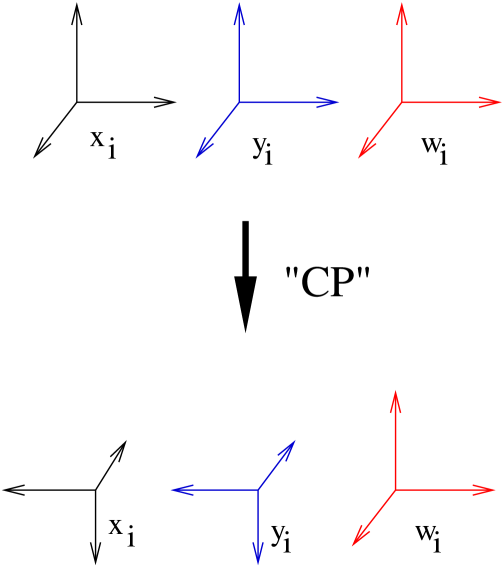
Figure 2: Rotations on 3 non-compact plus 3 compact directions corresponding to CP.

An even simpler picture holds for branes at orbifold fixed points, as we shall now see, and it is the geometric configuration of torsion plus singularity that breaks CP. As an example, consider the chiral multiplets written explicitly in eq.(34). The corresponding antiparticles are given by the conjugate excitation, and the projections are reversed accordingly;

$$\overline{\rho}.V_{\theta} = -v_{\theta,i}$$ (44)

$$\overline{\rho}.V_{\omega_{1}} = -v_{\omega_{1},i}$$ (45)

$$\Pi_{\omega_{2}}(\overline{\rho}) \rightarrow e^{-2\pi iv_{\omega_{2},i}}\overline{\rho},$$ (46)

giving

$$\overline{\rho}= [\underline{(+0..0)(0..0)^{n_{0}-1}}\underline{(-0..0)(0..0)^{n_{1}-1}}(0..0)^{n_{2}}]$$ (47)

$$+\,\,\,\varepsilon^{-1}[\underline{(0+0..0)(0..0)^{n_{0}-1}}\underline{(0-0..0)(0..0)^{n_{1}-1}}(0..0)^{n_{2}}]$$ (48)

$$+\,\,\,\varepsilon^{-2}[\underline{(00+0..0)(0..0)^{n_{0}-1}}\underline{(00-0..0)(0..0)^{n_{1}-1}}(0..0)^{n_{2}}] +...$$ (49)

as expected.

Now consider the rotation $x^{\mu}\rightarrow x_{\mu},$  $z_{i}\rightarrow z_{i}^{*}.$ Again by supersymmetry we transform $\psi_{i}\rightarrow\overline{\psi_{i}}$ and need to reverse the chiralities in the Ramond sector. The particle projections now trivially become antiparticle projections. To get the right antiparticles however, we also need to ensure that we have the same projective representation which is the case if the discrete torsion is unchanged (e.g. so that we have same linear combination as in eq.(47). If this were not the case we would simply be unable to identify these particular rotations with CP conjugation.) For open string sectors the effect of the torsion in a sector with $\mathbb{Z}_{M}\times\mathbb{Z}_{M}$ twists given by ($g\equiv a,b$ ; $h\equiv a^{\prime},b^{\prime}$) can be written as

$$\beta(g,h)=\epsilon^{ab^{\prime}-ba^{\prime}}.$$ (50)

The effect of the $z_{i}\rightarrow z_{i}^{*}$ reflection on the torsion in any sector is simply to reverse the twists, $(a,b\,;\,a^{\prime},b^{\prime}\,)$ $\rightarrow-(a,b\,;\,a^{\prime},b^{\prime}\,)$ so $\beta(g,h)$ is indeed unchanged and the rotation gives us the antiparticle. i.e. 4 dimensional CP conjugation does indeed correspond to a rotation in the 10D theory, with or without discrete torsion.

It is precisely because the discrete torsion is invariant under CP conjugation that the superpotential interactions are not. Indeed the superpotential is of the form

$$W=Tr(\Phi_{1}\Phi_{2}\Phi_{3}+\varepsilon^{-1/n}\Phi_{2}\Phi_{1}\Phi_{3}),$$ (51)

where here the $\Phi$’s stand for generic chiral fields, and where a summation over the SU(3) Levi-Cevita symbol is implied. Under the CP transformation we conjugate the chiral superfields but the discrete torsion remains the same. Thus

$$\int d\theta^{2}\,W+\int d\overline{\theta}^{2}\,\overline{W}\,\rightarrow\,\int d\overline{\theta}^{2}\,\overline{W}_{CP}+\int d\theta^{2}W_{CP}\,$$ (52)

where

$$W_{CP}=Tr(\Phi_{1}\Phi_{2}\Phi_{3}+\varepsilon^{1/n}\Phi_{2}\Phi_{1}\Phi_{3}).$$ (53)

So it is the discrete torsion term in the superpotential that is directly responsible for breaking 4 dimensional CP and, because CP conjugation is associated with a 10D Lorentz rotation, it is a spontaneously broken symmetry. We will now divert our attention to the more phenomenological issues.

3 Yukawas and the CKM matrix

In this section we first discuss some theoretical considerations for obtaining the canonical yukawa couplings. In particular, we derive bottom-up properties of the kähler metric that have not been previously noted. We then proceed to the CKM matrix and predictions for the CKM angles and quark mass ratios. Finally we discuss radiative corrections between the string and weak scales.

3.1 Normalisation of Yukawas

3.1.1 Bottom-up properties of the kähler metric

To be consistent with N=1 supersymmetry, we assume the low-energy effective field theory decribing our visible sector is an N=1 SUGRA theory. It is well known that in such a theory scalar fields have a non-canonical kinetic energy term given by a kähler metric which is a function of the compactification moduli. This normalistion of scalar fields, results in an effective normalisation of coupling constants. In particular, if we expand the kähler potential to first order in the charged matter fields, we have

$$\mbox{K}=\mbox{\^{K}}(M^{a},M^{a*})+\mbox{\~{K}}(M^{a},M^{a*})_{\alpha\beta}Tr(\Phi^{\alpha*}\Phi^{\beta})+...,$$ (54)

where $M^{a},M^{a*}$ are the closed string moduli fields and we obtain,

$$\hat{h}_{abc}=e^{\hat{K}/2}h_{lmn}(\mbox{\~{K}}^{-1/2})^{l}{}_{a}(\mbox{\~{K}}^{-1/2})^{m}{}_{b}(\mbox{\~{K}}^{-1/2})^{n}{}_{c},$$ (55)

where $\hat{h}_{abc}$ are the canonically normalised yukawa couplings. It is important to note that $\mbox{\~{K}}_{\alpha\beta}$ factorises into different components, one for each sector of the spectrum, e.g. in our case the 33 and 37 sector fields have the seperate kähler matter metrics, $(\mbox{\~{K}}_{33})_{\alpha\beta}$ and $(\mbox{\~{K}}_{37})_{\alpha\beta}$.

One of the strengths of the bottom-up approach is that, up until now, our discussion has been independent of any compactification scheme. In particular, the gauge group, SM spectrum and 3 generations of matter fields are all features independent of the global structure of the model. This affords us two approaches to the determination of the yukawas,

• Select a particular compactification and calculate the exact kähler potential.

• Choose an ansatz for $\mbox{\~{K}}_{33}$ and $\mbox{\~{K}}_{37}$ (note that the CKM matrix is independent of K̂).

The first approach is technically difficult and only acheivable in the simplest of cases, e.g. toroidal orbifolds. In addition, it goes against the bottom-up approach, which is to constrain the model as much as possible from the local rather than global properties. The second approach, at first sight, seems too arbitrary. However, the choice of possible ansätze is restricted by two observations. Firstly, the discrete torsion can constrain the form of $\mbox{\~{K}}_{33}$. Such a situation arises as a consequence of $Tr(\Phi_{33}^{\alpha*}\Phi_{33}^{\beta})$ containing a factor $Tr((X_{33}^{(\alpha)})^{\dagger}X_{33}^{(\beta)})$ arising from the Chan-Paton factors. This matrix contains ‘texture zeros’, dependent on the discrete torsion(n), which are inherited by $(\mbox{\~{K}}_{33})_{\alpha\beta}$. Note that the kähler metric is hermitian, and we will coventionally refer only to the zeros in the upper triangular section of $\mbox{\~{K}}_{33}$. There are three possible cases,

• minimal discrete torsion, i.e. $n=1$, with $\mbox{\~{K}}_{33}$ diagonal,

• $n=2$, with two off diagonal zeros,

• and $n\geq 3$, with no off diagonal zeros.

These results are derived in the appendices.

Finally, we have the restriction that $\mbox{\~{K}}_{37}$ is diagonal. $(\mbox{\~{K}}_{37})_{ij}$ can be calculated from tree-level modulus-matter scattering [29]. The amplitude is given by a disc diagram with two open string vertex operators on the boundary, a $(37_{i})$ and $(7_{j}3)$ vertex, and two closed string vertex operators attached to the interior, corresponding to the moduli fields. However vertices of $(37_{i})$ and $(7_{i}3)$ strings must come in pairs in order to get a consistent D-brane boundary on the disc. It follows that in this case i=j and hence $\mbox{\~{K}}_{37}$ is diagonal.

This allows us to explore possibilities for interesting flavour structure and CP violation in our yukawas without worrying about the exact compactification scheme we are using. That is, we choose an ansatz for the kähler metric based on our choice of discrete torsion, not our choice of compactification.

3.1.2 Explicit expressions for Yukawas

Defining the hermitian matrices,

$$\begin{array}[]{l}t_{33}=\mbox{\~{K}}_{33}^{-1},\\ t_{37}=\mbox{\~{K}}_{37}^{-1},\end{array}$$ (56)

and substituting into (55) we obtain, in the general case, canonical up-quark yukawas,

$$\begin{array}[]{l}\hat{h}^{abc}=e^{\hat{K}/2}h_{lmn}(t_{33}^{1/2})^{la}(t_{33}^{1/2})^{mb}(t_{33}^{1/2})^{nc}\\ =e^{\hat{K}/2}(\varepsilon_{lmn}+(1-e^{-2\pi i/M})s_{lmn})(t_{33}^{1/2})^{la}(t_{33}^{1/2})^{mb}(t_{33}^{1/2})^{nc}.\end{array}$$ (57)

Furthermore giving the three generation of Higgs fields vevs, $\langle h_{u}\rangle_{c}$, we obtain

$$(Y_{u})^{ab}=e^{\hat{K}/2}(\varepsilon_{lmn}+(1-e^{-2\pi i/M})s_{lmn})(t_{33}^{1/2})^{la}(t_{33}^{1/2})^{mb}(t_{33}^{1/2})^{nc}\langle h_{u}\rangle_{c}.$$ (58)

This expression also holds if we associate the actual physical Higgs fields with a linear combination of the $H_{u/d}^{a}$ fields. That is

$$\hat{H}_{u/d}^{i}=U_{u/d}^{ij}\tilde{H}_{u/d}^{j},$$ (59)

where $\hat{H}_{u/d}^{i}$ are the physical Higgs fields and $U_{u/d}$ is a unitary matrix. Then assuming that only $\hat{H}^{1}_{u/d}$ is light and the other two physical Higgs’ are heavy, we simply replace $\langle h_{u}\rangle_{c}$ with $(U_{u}^{\dagger})_{c1}$.

Similarly, for the down-quark yukawas, we obtain,

$$(Y_{d})^{ab}=e^{\hat{K}/2}\sum_{l=1}^{3}(t_{33}^{1/2})^{la}(t_{37}^{1/2})^{lb}(t_{37}^{1/2})^{lc}\langle h_{d}\rangle_{c}.$$ (60)

Using these formulae we can calculate the CKM matrix and determine the possiblities for CP violation in our model.

3.2 The CKM matrix

3.2.1 A simple ansatz from a choice of discrete torsion

Using the bottom-up properties of our kähler metric, that is,

• the zeros in $\mbox{\~{K}}_{33}$ are determined by the discrete torsion,

• $\mbox{\~{K}}_{37}$ is diagonal,

we try the following simple ansatz, take M=5, n=2 and

$$t_{33}^{\frac{1}{2}}=\left(\begin{array}[]{ccc}\eta\alpha\varepsilon^{2}&0&\alpha\varepsilon\\ 0&1&0\\ \alpha\varepsilon&0&\alpha\end{array}\right),$$ (61)

$$t_{37}^{\frac{1}{2}}=diag[1,\varepsilon,1],$$ (62)

$$\begin{array}[]{ll}\langle h_{u}\rangle=&(\varepsilon,1,0),\\ \langle h_{d}\rangle=&(1,\varepsilon,\varepsilon).\end{array}$$ (63)

Notice that our choice of discrete torsion introduces two off diagonal zeros in $\mbox{\~{K}}_{33}$ which are preserved in $t_{33}^{\frac{1}{2}}$.

Using this ansatz we can calculate the Yukawas and CKM matrix. The Yukawas have the following form,

$$Y_{u}=\alpha^{2}\varepsilon\left(\begin{array}[]{lcl}(1-e^{-2i\pi/5})\eta\varepsilon^{2}&(1-e^{-2i\pi/5})\eta\varepsilon^{3}&(1-\eta e^{-2i\pi/5})\varepsilon\\ (1-e^{-2i\pi/5})\eta\varepsilon^{3}&0&(\eta-e^{-2i\pi/5})\varepsilon^{2}\\ (\eta-e^{-2i\pi/5})\varepsilon&(1-\eta e^{-2i\pi/5})\varepsilon^{2}&(1-e^{-2i\pi/5})\end{array}\right),$$ (64)

and

$$Y_{d}=\alpha\varepsilon\left(\begin{array}[]{lll}\eta\varepsilon&0&\varepsilon\\ 0&\frac{\varepsilon^{2}}{\alpha}&0\\ 1&0&1\end{array}\right).$$ (65)

With the freedom to rephase the right handed quark fields (because the model is supersymmetric we can make rephasings just as in the Standard Model), $Y_{u}$ can be put into hermitian form. Notice that $\alpha$ appears only as an overall factor in $Y_{u}$ and in a single entry in $Y_{d}$, as a consequence the CKM matrix is only dependent on the two parameters $\varepsilon$ and $\eta$, with $\alpha$ determining the mass of the down quark. Up to overall factors, which include the prefactors of (64) and (65), the masses of the quarks are given approximately for small $\eta$ and $\varepsilon$ by,

$$\begin{array}[]{lll}m_{d}=\frac{\varepsilon^{2}}{\alpha},&m_{s}=\frac{\varepsilon(1-\eta)}{\sqrt{2}},&m_{b}=\sqrt{2}+\frac{1}{4\sqrt{2}}\varepsilon^{2}+\frac{1}{20\sqrt{2}}\eta\varepsilon^{2},\\ m_{u}=1.9\eta\varepsilon^{4},&m_{c}=\sqrt{\frac{2}{3}}\varepsilon^{2}-\frac{\sqrt{26}}{3}\eta\varepsilon^{2}+\sqrt{\frac{2}{3}}\eta^{2}\varepsilon^{2},&m_{t}=\frac{2}{\sqrt{3}}+\sqrt{\frac{2}{3}}\varepsilon^{2}-\frac{1}{\sqrt{3}}\eta\varepsilon^{2}.\end{array}$$ (66)

The CKM matrix can be written approximately in terms of these mass eigenvalues, but it is not very illuminating to show the functional dependence here. Instead, in the next subsection, we depict graphically it’s functional dependence on $\varepsilon$ and $\eta$.

3.2.2 Predictions: CKM angles and Quark mass ratios

In the standard parametrisation, the CKM matrix is given in terms of three mixing angles, $\sin{\theta_{12}}$, $\sin{\theta_{23}}$, $\sin{\theta_{13}}$, and a complex phase $\delta$. Figures 3 to 6 illustrate the dependence of these CKM angles on $\varepsilon$ and $\eta$. The blue shaded areas highlight the regions where the CKM angles agree with experiment [30]. Since we are discussing string scale predictions we must also include RGE effects in running from the string to the weak scale. This effect is discussed in the next subsection, where we estimate that $\sin{\theta_{23}}$ and $\sin{\theta_{13}}$ are suppressed by approximately $30\%$. This is depicted in the figures by a red shaded region which higlights values of $\varepsilon$ and $\eta$ that will reproduce experimental values after taking into account RGE effects. This information is summarised in figure 7 where the regions in parameter space which produce a realistic CKM matrix are highlighted. In particular, it can be seen that $\delta$ is approximately $\pi/3$.

The quark mass ratios are also determined, $\frac{m_{d}}{m_{b}}$ can be fixed by choosing a value for $\alpha$, while the rest of the quark mass ratios are dependent only on $\varepsilon$ and $\eta$. Average values for the blue and red regions are presented in table 1 and compared to experimental values. As can be seen, we have good agreement with experiment except for $\frac{m_{u}}{m_{c}}$ which is too large. Note that we have not included RGE effects here, which would tend to increase the value of $\frac{m_{c}}{m_{t}}$. As we have chosen such a constrained and simple ansatz, we consider the close agreement of the CKM angles and quark mass ratios with experiment to be successful. Furthermore, it has not been necessary to introduce any large artificial hierarchies in our ansatz (which would require similar hierarchies in the corresponding moduli fields), to achieve mass eigenvalues and mixing angles close to those of the Standard Model.

Figure 3: $\sin{\theta_{12}}$ as a function of $\varepsilon$ and $\eta$.

Figure 4: $\sin{\theta_{13}}$ as a function of $\varepsilon$ and $\eta$.

Figure 5: $\sin{\theta_{23}}$ as a function of $\varepsilon$ and $\eta$.

Figure 6: $\delta/\pi$ as a function of $\varepsilon$ and $\eta$.

Figure 7: The shaded regions highlight the values of $\varepsilon$ and $\eta$ which give an agreement with experimental data. The blue/red region without/with taking into account RGE effects.

Mass Ratio	Blue Region	Red Region	Experimental Value
$\frac{m_{c}}{m_{t}}$	$2.5\times 10^{-3}$	$5\times 10^{-3}$	$5.57-8.27\times 10^{-3}$
$\frac{m_{s}}{m_{b}}$	$0.029$	$0.041$	$0.018-0.0387$
$\frac{m_{u}}{m_{c}}$	$2.4\times 10^{-2}$	$2.1\times 10^{-2}$	$1.07-4.5\times 10^{-3}$

Table 1: Quark mass ratios

3.2.3 RGE effects

The CKM matrix is expected to be effected by renormalization group running. For instance, when we are close to the so-called quasifixed point, the top Yukawa is large at the GUT or string scale and runs to lower fixed point values, and hence RGE effects are important.

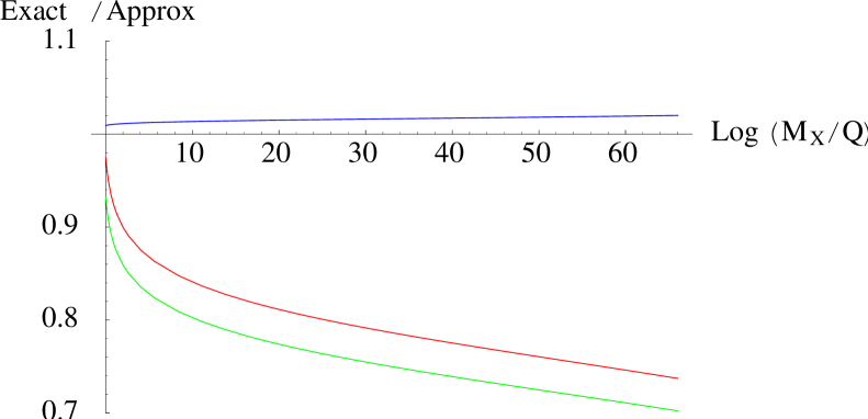
Figure 8: CKM running from $M_{X}\approx 2\times 10^{16}GeV$ to $M_{W}$ for a top Yukawa of $\lambda_{t}=5$ at the GUT scale. Where red $\equiv\frac{\sin\theta_{23}}{(\sin\theta_{23})_{GUT}}$, blue $\equiv\frac{\frac{\sin\theta_{13}}{\sin\theta_{12}}}{(\frac{\sin\theta_{13}}{\sin\theta_{12}})_{GUT}}$, green $\equiv\frac{\delta}{\delta_{GUT}}$. $\sin\theta_{12}$ does not run significantly.

However, the effect on the CKM angles is generally small, as can be seen by inspection of the RG equation. Figure 8 shows how the numerical values of the CKM parameters change with renormalization scale when the top quark Yukawa is close to the quasifixed point. The CKM angles are suppressed by the running and from the figure we see that the maximum reasonable suppression of the $\theta_{23}$ and $\theta_{13}$ angles is $\approx 30\%$. The phase $\delta$ does not change significantly and is expected to be close to $\frac{\pi}{3}$.

4 Summary and discussion

We have presented a bottom-up supersymmetric D-brane model with phenomenologically viable CP violation, broken by discrete torsion. Furthermore, a simple assumption about the form of the kähler metric, motivated by a choice of discrete torsion, produces a CKM matrix described by only two free parameters. As a consequence, we predict a single CKM mixing angle and the CKM phase to be close to $\pi/3$, both of which lie within current experimental limits. We believe this to be the first such prediction from any string model.

We believe that this class of models may be a first step towards a solution of the SUSY flavour and CP problems. Generally, these problems arise because supersymmetry breaking “knows” about CP and flavour. The approach that we favour is therefore to use the ‘bottom-up’ approach to build a supersymmetric MSSM, complete with all flavour and CP structure, before discussing supersymmetry breaking.

An interesting hint may lie in the fact that the Yukawa structure in these models seems to favour a hermitian flavour structure. Hermiticity has been suggested as a way to combat large EDMs and solve the SUSY CP problem [31]. In our analysis only the up-quark Yukawas are hermitian and so we cannot yet claim to have a solution. However we think that the appearance of hermitian flavour structure is intriguing.

It would be interesting to investigate the dependence of these results on our choice of discrete torsion (i.e. our choice of $n$), and the resulting ansatz for the kähler metrics. Finally an analysis of the possibilities for a phenomenologically viable breaking of supersymmetry has been well motivated. All of these questions will be the subject of future work.

5 Acknowledgements

We would like to thank Shaaban Khalil for assistance with computations. S.A.Abel is supported by a PPARC Opportunity grant and A.W.Owen by a PPARC studentship.

Appendix

Appendix A Calculation of Chan-Paton factors

Consider a generic chiral superfield whose Chan-Paton factor, as a result of the $\gamma_{\theta}$ projection, is of size $sn^{(i)}\times sn^{(j)}$. If we act on this state with an element $g=(a,b)=\omega_{1}^{a}\omega_{2}^{b}\in\mathbb{Z}_{M}\times\mathbb{Z}_{M}$, we require 

$$\lambda_{sn^{(i)}\times sn^{(j)}}^{(k)}=r^{(k)}(a,b)\gamma_{g,3}\lambda_{sn^{(i)}\times sn^{(j)}}^{(k)}\gamma_{g,3}^{\dagger},$$ (67)

where $r^{(k)}(a,b)$ is a phase from the action on the string worldsheet fields and for a string endpoint on a set of $sn^{(i)}$ D-branes,

$$\gamma_{g}=\oplus_{l,m}(\sqrt{\epsilon})^{-ab}(\omega_{M}^{l}\gamma_{\omega_{1}})^{a}(\omega_{M}^{m}\gamma_{\omega_{2}})^{b}\otimes I_{n^{(i)}_{lm}},$$ (68)

where $\omega_{M}=e^{2\pi i/M}$, $\sum_{l,m}n^{(i)}_{lm}=n^{(i)}$ and $l,m=0,...,(M/s)-1$. It follows that we can factor the Chan-Paton matrix by writing,

$$\lambda^{(k)}_{sn^{(i)}\times sn^{(j)}}=\oplus_{l,m}X^{(k)}_{s\times s}\otimes Y^{(k)}_{n^{(i)}_{lm}\times n^{(j)}_{lm}}.$$ (69)

where $X^{(k)}$ is determined by the action of $\mathbb{Z}_{M}\times\mathbb{Z}_{M}$ and $Y^{(k)}$ is left undetermined. Substituting (69) into (67) removes the dependence on $Y^{(k)}$ giving,

$$X^{(k)}\gamma_{\omega_{1}}^{a}\gamma_{\omega_{2}}^{b}=r^{(k)}(a,b)\gamma_{\omega_{1}}^{a}\gamma_{\omega_{2}}^{b}X^{(k)}.$$ (70)

Since the $\gamma_{\omega_{i}}$ matrices form a projective representation and hence satisfy $\gamma_{g}\gamma_{h}=\beta(g,h)\gamma_{h}\gamma_{g}$, we can solve (70) with the ansatz $X^{(k)}=\gamma_{\omega_{1}}^{p_{k}}\gamma_{\omega_{2}}^{q_{k}}$. This results in,

$$\beta(\omega_{1},\omega_{2})^{p_{k}b-q_{k}a}=r^{(k)}(a,b).$$ (71)

For 33 sector fields we have,

$$r_{33}^{(k)}(a,b)=e^{2\pi i(av_{\omega_{1}}+bv_{\omega_{2}})},$$ (72)

and for 37 sector fields we have,

$$r_{37}^{(k)}(a,b)=e^{\pi i(a\sum_{i\neq k}v_{\omega_{1}}^{i}+b\sum_{i\neq k}v_{\omega_{2}}^{i})}.$$ (73)

Substituting these expressions into (71) we find,

$$\begin{array}[]{l}p_{k}=\left\{\begin{array}[]{ll}\frac{a_{2}^{k}}{n}&\mbox{For 33 fields}\\ \frac{1}{2n}\sum_{i\neq k}a_{2}^{i}&\mbox{For 37 fields}\end{array}\right.,\\ q_{k}=\left\{\begin{array}[]{ll}-\frac{a_{1}^{k}}{n}&\mbox{For 33 fields}\\ -\frac{1}{2n}\sum_{i\neq k}a_{1}^{i}&\mbox{For 37 fields}\end{array}\right.,\\ \end{array}$$ (74)

where $v_{\omega_{i}}=\frac{1}{M}(a_{i}^{1},a_{i}^{2},a_{i}^{3})$. Finally we have, for the 33 fields,

$$\begin{array}[]{lll}X^{(1)}_{33}=\gamma_{\omega_{2}}^{-\frac{1}{n}},&X^{(2)}_{33}=\gamma_{\omega_{1}}^{\frac{1}{n}}\gamma_{\omega_{2}}^{\frac{1}{n}},&X^{(3)}_{33}=\gamma_{\omega_{1}}^{-\frac{1}{n}},\end{array}$$ (75)

and for the 37 fields,

$$\begin{array}[]{lll}X_{37_{1}}=\gamma_{\omega_{2}}^{\frac{1}{2n}},&X_{37_{2}}=\gamma_{\omega_{1}}^{-\frac{1}{2n}}\gamma_{\omega_{2}}^{-\frac{1}{2n}},&X_{37_{3}}=\gamma_{\omega_{1}}^{\frac{1}{2n}}.\end{array}$$ (76)

Appendix B Determination of zeros in $\mbox{\~{K}}_{33}$

As discussed in the main text, the zeros in $\mbox{\~{K}}_{33}$ are inherited from the hermitian matrix,

$$Z_{ij}=Tr((X^{(i)}_{33})^{\dagger}X^{(j)}_{33}).$$ (77)

However, equation (75) does not determine the $X^{(i)}_{33}$ uniquely. Therefore, we choose the $\mbox{n}^{th}$ principal root of $\gamma_{\omega_{k}}$ defined by,

$$\gamma_{\omega_{k}}^{\frac{1}{n}}=S^{\dagger}(\gamma_{\omega_{k}}^{diag})^{\frac{1}{n}}S,$$ (78)

with S the unitary matrix which diagonalises $\gamma_{\omega_{k}}$ and,

$$(\gamma_{\omega_{k}}^{diag})_{ij}=\delta_{ij}\lambda_{i}^{\frac{1}{n}}.$$ (79)

Here $\lambda_{i}$ is the $i^{th}$ eigenvalue of $\gamma_{\omega_{k}}$, $\lambda_{i}^{1/n}\equiv e^{\frac{1}{n}\log(\lambda_{i})}$ and we restrict $\arg(\lambda_{i})$ to the interval $(-\pi,\pi]$, thus taking the principal value of $\log(\lambda_{i})$.

With these choices, the $X^{(i)}_{33}$ are uniquely determined and we have,

$$\begin{array}[]{ll}Z_{12}=&\frac{1}{s}(\sum_{l=1}^{g(s)}e^{-4\pi i(l-1)/ns}+e^{4\pi i/n}\sum_{l=g(s)+1}^{s}e^{-4\pi i(l-1)/ns})\\ &\times(\sum_{p=0}^{p_{max}}e^{2\pi ip/n}\sum_{u(p)>j\geq l(p)}e^{-2\pi i(j-1)/M}),\end{array}$$ (80)

$$\begin{array}[]{ll}Z_{13}=&\frac{1}{s}(\sum_{l=1}^{g(s)}e^{-2\pi i(l-1)/ns}+e^{2\pi i/n}\sum_{l=g(s)+1}^{s}e^{-2\pi i(l-1)/ns})\\ &\times(\sum_{p=0}^{p_{max}}e^{-2\pi ip/n}\sum_{u(p)>j\geq l(p)}e^{2\pi i(j-1)/M}),\end{array}$$ (81)

and,

$$\begin{array}[]{ll}Z_{23}=&\frac{1}{s}(\sum_{l=1}^{g(s)}e^{2\pi i(l-1)/ns}+e^{-2\pi i/n}\sum_{l=g(s)+1}^{s}e^{2\pi i(l-1)/ns})\\ &\times(\sum_{p=0}^{p_{max}}e^{-4\pi ip/n}\sum_{u(p)>j\geq l(p)}e^{4\pi i(j-1)/M}),\end{array}$$ (82)

where,

$$\begin{array}[]{l}p_{max}=[\frac{(s-1)n}{M}+\frac{1}{2}],\\ u(p)=(2p+1)\frac{M}{2n}+1,\\ l(p)=(2p-1)\frac{M}{2n}+1,\\ g(s)=\left\{\begin{array}[]{ll}k&\mbox{if s=2k,}\\ k+1&\mbox{if s=2k+1,}\end{array}\right.\end{array}$$ (83)

with $[..]$ denoting rounding to the nearest integer. Furthermore, since the $X^{(i)}_{33}$ are unitary $s\times s$ matrices, we have

$$Z=\left(\begin{array}[]{ccc}s&Z_{12}&Z_{13}\\ Z_{12}^{*}&s&Z_{23}\\ Z_{13}^{*}&Z_{23}^{*}&s\end{array}\right).$$ (84)

Finally, it can be easily seen from (80), (81) and (82) that $Z_{12}=Z_{13}=Z_{23}=0$ for $n=1$, $Z_{12}=Z_{23}=0$ and $Z_{13}\neq 0$ for $n=2$ and for $n\geq 3$ all elements of Z are non-zero. Hence giving rise to the three distinct cases for the distribution of zeros in $\mbox{\~{K}}_{33}$ as described in the main text.

References

• [1] B.Aubert et al. Observation of CP Violation in the B0 Meson System. Phys.Rev.Lett, 87:091801. hep-ex/0107013.
• [2] K.Abe et al. Observation of Large CP Violation in the Neutral B Meson System. Phys.Rev.Lett, 87:091802. hep-ex/0107061.
• [3] T.Affolder et al. A Measurement of $\sin 2\beta$ from B $\rightarrow$ J / ${\Psi}$ K0(S) with the CDF Detector. Phys.Rev., D61:072005. hep-ex/9909003.
• [4] M.Dine, R.G.Leigh, and D.A.MacIntire. Of CP and other Gauge Symmetries in String theory. Phys.Rev.Lett, 69:2030–2032, 1992. hep-th/9205011.
• [5] K.Choi, D.B.Kaplan, and A.E.Nelson. Is CP a Gauge Symmetry? Nucl.Phys., B391:515, 1993. hep-ph/9205202.
• [6] S.Khalil, O.Lebedev, and S.Morris. CP Violation and Dilaton Stabilization in Heterotic String Models. Phys.Rev., D65:115014, 2002. hep-th/0110063.
• [7] O.Lebedev and S.Morris. Towards a Realistic Picture of CP Violation in Heterotic String Models. JHEP, 0208:007, 2002. hep-th/0203246.
• [8] S.A.Abel and G.Servant. CP and Flavour in Effective Type I Strings Models. Nucl.Phys., B611:43. hep-ph/0105262.
• [9] S.A.Abel and G.Servant. Dilaton Stabilization in Effective Type I String Models. Nucl.Phys., B597:3. hep-th/0009089.
• [10] D.Bailin, G.V.Kraniotis, and A.Love. The Effect of Wilson Line Moduli on CP Violation by Soft Supersymmetry Breaking Terms. Phys.Lett, B422:343–352. hep-th/98041325.
• [11] D.Bailin, G.V.Kraniotis, and A.Love. CP Violating Phases in the CKM Matrix in Orbifold Compactifications. Phys.Lett, B435:323–330. hep-th/9805111.
• [12] D.Bailin, G.V.Kraniotis, and A.Love. CP Violation by Soft Supersymmetry Breaking terms in Orbifold Compactifications. Phys.Lett, B414:269. hep-th/9707105.
• [13] T.Dent. Breaking CP and Supersymmetry with Orbifold Moduli Dynamics. Nucl.Phys., B623:73–96. hep-th/0110110.
• [14] G.Aldazabal, L.E.Ibáñez, F.Quevedo, and A.M.Uranga. D-branes at Singularities: A Bottom-Up Approach to the String Embedding of the Standard Model. JHEP, 008:002, 2000. hep-th/0005067.
• [15] E.Sharpe. Recent Developments in Discrete Torsion. Phys.Lett., B498:104–110, 2002. hep-th/0008191.
• [16] A. Masiero and T. Yanagida. Real CP Violation. hep-ph/9812225.
• [17] R.N.Mohapatra and A.Rasin. Simple Supersymmetric Solution to the Strong CP Problem. Phys.Rev.Lett, 76:3490–3493. hep-ph/9511391.
• [18] S.Abel, D. Bailin, S. Khalil, and O. Lebedev. Flavor Dependent CP Violation and Natural Suppression of the Electric Dipole Moments. Phys.Lett, B504:241–246. hep-ph/0012145.
• [19] S.Khalil. CP Violation in Supersymmetric Models with Hermitian Yukawa couplings and A-terms. hep-ph/0202204.
• [20] R.N.Mohapatra and G.Senjanovic. Natural Supression of Strong P and T non-invariance. Phys.Lett., B79:283.
• [21] M.R.Douglas. D-branes and Discrete Torsion. hep-th/9807235.
• [22] M.Klein and R.Rabadán. Orientifolds with Discrete Torsion. JHEP, 0007:040, 2000. hep-th/0002103.
• [23] C.Vafa. Modular Invariance and Discrete Torsion in Orbifolds. Nucl. Phys, B273:592–606, 1986.
• [24] C.Vafa and E.Witten. On Orbifolds with Discrete Torsion. J.Geom.Phys, 15:189–214. hep-th/9409188.
• [25] G.Aldazabal, A.Font, L.E.Ibáñez, and A.M.Uranga. String GUTs. Nucl.Phys., B452:3, 1995. hep-th/9706158.
• [26] G.Aldazabal, A.Font, L.E.Ibáñez, A.M.Uranga, and G.Violero. Non-perturbative Heterotic D=6, N=1 Orbifold Vacua. Nuclear Physics, B519:239. hep-th/9706158.
• [27] G.Aldazabal, A.Font, L.E.Ibáñez, and G.Violero. D=4, N=1, Type IIB Orientifolds. Nucl.Phys., B536:29–68. hep-th/9804026.
• [28] M.Berkooz and R.G.Leigh. A D=4 N=1 Orbifold of Type I Strings. Nucl.Phys., B483:187–208, 1997. hep-th/9605049.
• [29] V.Kaplunovsky and J.Louis. On Gauge Couplings in String Theory. Nucl.Phys., B444:191–244, 1995. hep-th/9502077.
• [30] K.Hagiwara et al. Particle Data Group. Phys.Rev., D66:010001, 2002.
• [31] S.Abel, S.Khalil, and O.Lebedev. The String CP problem. hep-ph/0112260.