TPI-MINN 02/12

UMN-TH-2052/02

PNPI-TH-2474/02

ITEP-TH-23/02

Metastable Strings in Abelian Higgs Models Embedded in Non-Abelian Theories: Calculating the Decay Rate

M. Shifman^a and Alexei Yung^a,b,c

^aTheoretical Physics Institute, University of Minnesota, Minneapolis, MN 55455, USA
^bPetersburg Nuclear Physics Institute, Gatchina, St. Petersburg 188300, Russia
^cInstitute of Theoretical and Experimental Physics, Moscow 117250, Russia

Abstract

We study the fate of U(1) strings embedded in a non-Abelian gauge theory with the hierarchical pattern of the symmetry breaking: ${G}\stackrel{{\scriptstyle V}}{{\longrightarrow}}{\rm U(1)}\stackrel{{\scriptstyle v}}{{\longrightarrow}}{\rm nothing}$, $V\gg v$. While in the low-energy limit the Abrikosov-Nielsen-Olesen string (flux tube) is perfectly stable, being considered in the full theory it is metastable. We consider the simplest example: the magnetic flux tubes in the SU(2) gauge theory with adjoint and fundamental scalars. First, the adjoint scalar develops a vacuum expectation value $V$ breaking SU(2) down to U(1). Then, at a much lower scale, the fundamental scalar (quark) develops a vacuum expectation value $v$ creating the Abrikosov-Nielsen-Olesen string. (We also consider an alternative scenario in which the second breaking, ${\rm U(1)}\stackrel{{\scriptstyle v}}{{\longrightarrow}}{\rm nothing}$, is due to an adjoint field.) We suggest an illustrative ansatz describing an “unwinding” in SU(2) of the winding inherent to the Abrikosov-Nielsen-Olesen strings in U(1). This ansatz determines an effective 2D theory for the unstable mode on the string world-sheet. We calculate the decay rate (per unit length of the string) in this ansatz and then derive a general formula. The decay rate is exponentially suppressed. The suppressing exponent is proportional to the ratio of the monopole mass squared to the string tension, which is quite natural in view of the string breaking through the monopole-antimonopole pair production. We compare our result with the one given by Schwinger’s formula dualized for describing the monopole-antimonopole pair production in the magnetic field.

1 Introduction

Formation of the chromoelectric flux tubes in non-Abelian gauge theories is being discussed as a mechanism of color confinement, at a qualitative level, since the early days of quantum chromodynamics (QCD). No quantitative first-principle description of the phenomenon was ever constructed in QCD — strong coupling regime inherent to this theory precluded all efforts in this direction.

The revival of interest to non-Abelian gauge theories occurred in the mid-1990’s. The idea of using supersymmetry as a tool allowing one to deal, to a certain extent, with strong coupling regime was revived. This development culminated in the work of Seiberg and Witten [1, 2] who considered ${\cal N}=2$ Yang-Mills theory slightly perturbed by a (small) mass term of the adjoint matter field. This perturbation breaks ${\cal N}=2$ down to ${\cal N}=1$. Supersymmetry proved to be sufficiently powerful to allow Seiberg and Witten to constructively demonstrate the existence of the dual Meissner effect — the monopole condensation accompanied by the formation of the chromoelectric flux tubes. Technically, the Seiberg-Witten theory has two distinct scales (this was crucial for their construction): the scale of strong interaction $\Lambda$, and a much smaller scale regulated by a small adjoint mass term. Below $\Lambda$ the original SU(2) Yang-Mills theory reduces to an Abelian (dual) quantum electrodynamics (QED). Correspondingly, the flux tubes (strings) of the Seiberg-Witten theory are the conventional U(1) Abrikosov-Nielsen-Olesen (ANO) strings [3, 4, 5]. In the SU($N$) case, the low-energy effective theory is that of U(1)^N-1; the flux tubes one deals with present a straightforward generalization of the ANO strings.

In the Yang-Mills theory without quarks, the underlying gauge group has a non-trivial $\pi_{1}$ homotopy. On topological grounds one then expects $Z_{N}$ vortices to appear [6, 7, 8, 9, 10, 11]. However, in fact, in the Seiberg-Witten construction, in which at low energies the gauge group is broken down to U(1)^N-1 by the adjoint matter condensation, it is the U(1)^N-1 strings that appear [12] near the monopole/dyon vacua. They form $N-1$ infinite towers of the ANO flux tubes for each of U(1) factors and give rise to confinement of quarks. It is clear that only some of these strings (those which correspond to $Z_{N}$ strings of the microscopic non-Abelian theory) are stable, all others must be unstable (metastable) [13] beyond the extreme low-energy limit.

A slightly different scenario takes place in the Seiberg-Witten theory with fundamental matter (quarks). In this case the underlying gauge group SU($N$) has a trivial homotopy group, $\pi_{1}({\rm SU}(N))=0$, and does not admit flux tubes. However, near the charge vacua this theory has an Abelian low-energy description too, which ensures the presence of the ANO flux tubes in the extreme low-energy limit. These ANO strings give rise to confinement of monopoles [14, 15, 16, 17]. It is perfectly clear that all these ANO strings must be metastable in the microscopic non-Abelian theory.

Thus, we see that the following general question presents a considerable interest. Assume that one considers an underlying non-Abelian gauge theory with a trivial (or “almost trivial”) homotopy group $\pi_{1}$. (For definiteness, one may choose SU(2).) Assume that this theory experiences a two-stage spontaneous symmetry breaking: first, at a high scale $V$, the non-Abelian group is broken down to an Abelian subgroup (let us say, U(1), for definiteness), and then this U(1), in turn, is spontaneously broken at a much lower scale $v$. The underlying non-Abelian theory will be referred to as “microscopic,” while the low-energy Abelian theory will be called “macroscopic.” In the low-energy limit one can forget about the microscopic theory and consider QED with a charged matter field which develops a vacuum expectation value (VEV). Correspondingly, stable ANO strings do exist in the macroscopic theory. In the microscopic theory they are metastable, rather than stable, however, because of the triviality of $\pi_{1}$ of the original gauge group. A long ANO string can (and will) break due to the monopole-antimonopole pair creation. The task is to find the probability (per unit length per unit time) of the string breaking.

This question can be quantitatively addressed at weak coupling. In this paper we consider a simple (non-supersymmetric) model which closely follows the pattern of the (supersymmetric) Seiberg-Witten theory. We start from an SU(2) gauge model with scalar fields — one in the adjoint and another in the fundamental representation — with a certain interaction between them. The field in the fundamental representation will be referred to as the “quark field.” The interaction of scalars is arranged in such a way that the adjoint scalar develops a large vacuum expectation value,

$$V\gg\Lambda\,,$$ (1.1)

where $\Lambda$ is the dynamical scale of the SU(2) theory. This VEV of the adjoint field breaks the SU(2) gauge group down to U(1) and ensures that the theory at hand is weakly coupled. At this stage the ’t Hooft-Polyakov monopoles emerge [18, 19]. Their mass is very heavy, $M_{M}\sim V/g$. Below scale $V$ one is left with QED. The (charged) quark field develops a small VEV $v$,

$$v\ll V\,.$$ (1.2)

Then the standard ANO flux tubes emerge. We study their decay in the quasiclassical approximation. To this end we consider dynamics of an unstable mode associated with the possibility of “unwinding” the ANO string winding on the SU(2) group manifold. This is an under-barrier process, with the corresponding action being very large in the limit $v\ll V$. The physical interpretation of this tunneling process is the monopole-antimonopole pair creation accompanied by annihilation of a segment of the string.

We present an analytic ansatz which explicitly “unwinds” the string. The string decay rate is found in the framework of this ansatz. Our task — constructing fully analytic ansatz — is admittedly illustrative. Therefore, we limit ourselves to a minimal number of profile functions. The ansatz obtained in this way is suitable for a qualitative understanding of the phenomenon. It is too restrictive to describe the production of the monopoles per se; rather, it describes the production of a pair of highly excited states with the monopole (antimonopole) quantum numbers. We argue, however, that an effective description of the string decay suggested by this ansatz is more general and is applicable for realistic ansätze provided that (i) the condition (1.2) is met, and (ii) the string tension and the monopole mass are treated as given parameters. In terms of these parameters the general result for the metastable string decay rate (the probability per unit time per unit length of the string) is

$$\Gamma_{\rm breaking}\sim v^{2}\,\exp\left\{-\,\frac{\pi\,\,M_{M}^{2}}{T_{\rm ANO}}\right\}\,,$$ (1.3)

where $M_{M}$ is the monopole mass and $T_{\rm ANO}$ is the string tension. It is worth reminding that $M_{M}^{2}\sim V^{2}/g^{2}$ while $T_{\rm ANO}\sim v^{2}$.

As was expected, $\Gamma_{\rm breaking}$ turns out to be exponentially suppressed. This is natural in light of the tunneling interpretation of the string breaking process — that the string is broken into pieces by the monopole-anti-monopole pair production. In fact, our result is quite similar to Schwinger’s formula [20] dualized to the magnetic charge production in the constant magnetic field [21]. The only difference is the replacement of $Bg^{-2}$ in the dualized Schwinger formula by $T_{\rm ANO}$. This is not surprising: the macroscopic theories of these two phenomena are similar.

The result presented in Eq. (1.3) is not new. It was obtained long ago in Refs. [22, 23]. In these papers the decay of metastable ANO strings arising in theories with a hierarchical pattern of symmetry breaking was treated in the framework of an effective theory, by calculating the action of the bubble formed by the monopole world line on the string world sheet.

In our present paper the logic is different. We “forget” for a while about monopoles per se, and use an “unwinding” ansatz to derive a quasi-modulus theory for the unstable string mode on the string world sheet. We then consider the bubble creation in this quasi-modulus theory and rederive Eq. (1.3). After this is done, we interpret (1.3) as the probability of the monopole-antimonopole pair production. From this standpoint our results can be viewed as a demonstration of the assertion that the “unwinding” of a metastable string goes via the production of the monopole-antimonopole pairs. We thus provide a necessary background for the effective approach formulated in the pioneering works [22, 23].

If the small-VEV field of the quark type (i.e. in the fundamental representation) is replaced by a small-VEV field in the adjoint (such that the VEV’s of two adjoint fields present in this model are misaligned), then one arrives at a weak coupling model of $Z_{2}$ strings. The gauge symmetry of the microscopic theory is now SU(2)/ $Z_{2}$. Since $\pi_{1}(\mbox{SU(2)/}Z_{2})=Z_{2}$ , the minimal magnetic flux string is absolutely topologically stable. Higher-flux strings are stable only in the low-energy U(1) limit, and can decay through the monopole-antimonopole pair production. We construct an “unwinding” ansatz in this case too, and argue that the decay rate is given by the same expression (1.3).

The paper is organized as follows. In Sect. 2 we formulate our model and explain, in concrete terms, what needs to be done in order to calculate the string decay probability. In Sect. 4 we present an ansatz for the gauge and scalar fields describing the under-barrier transition (“unwinding”) under consideration. The decaying string ansatz is parametrized by three profile functions. We identify an unstable mode $\theta$ in which tunneling occurs. For the extreme type II and type I strings one needs to know only the asymptotic behavior of the above profile functions. This simplifies the problem immensely.

Section 5 is devoted to the extreme type II string which arises in the theory with the quark mass much larger then the photon mass ($m_{q}\gg m_{\gamma}$). In this limit, the stable ANO solution was obtained analytically by Abrikosov long ago [3]. We generalize this solution to cover the decaying string. For the unstable mode $\theta$ we derive an effective two-dimensional field theory on the string world-sheet. The string breaking in the microscopic theory corresponds to the false vacuum decay in the effective world-sheet field theory for $\theta(t,z)$. We then apply well-developed methods [24, 25] for calculating the false vacuum decay rate through bubble formation. In this way we find the probability of the string breaking for the extreme type II strings.

In Sect. 6 we consider the opposite case of the extreme type I string ($m_{q}\ll m_{\gamma}$). The analytic solution in this case was obtained quite recently in Ref. [15]. Although the string tension for type I is given by an expression significantly different from that for type II, the string decay rate, being expressed in terms of the string tension, is determined by the same formula as in the type II case.

In Sect. 7 we turn to the theory with two adjoint scalars and work out the decay rate of the string with winding number $n=2$. Note, that the string with minimal winding number $n=1$ ($Z_{2}$-string) is stable in this model. Section 8 extends the proof of Eq. (1.3) to non-extreme strings.

In Sect. 9 we compare our result for the string decay rate with the one given by Schwinger’s formula [20] which might be used for the evaluation of the probability of the monopole-antimonopole pair production in the external magnetic field. The comparison can be performed only qualitatively.

The reason is that Schwinger’s formula and Eq. (1.3) refers to different phases of the theory. Schwinger’s formula deals with the monopole production in the external magnetic field in the Coulomb phase, while Eq. (1.3) describes breaking of ANO string by monopole-anti-monopole pair in the phase in which monopoles are confined. Still, the comparison exhibits a qualitative agreement with result (1.3) as far as the powers of the mass scales in the exponent are concerned.

Finally, Sect. 10 summarizes our results and conclusions and outlines problems for future investigation. Appendix contains some details of an “improved” unwinding ansatz.

2 The model and formulation of the problem

In the bulk of the paper we will consider SU(2) gauge theory with the action

$$S=\int d^{4}x\left\{\frac{1}{4g^{2}}F_{\mu\nu}^{a}F^{\mu\nu\,a}+\frac{1}{2}(D_{\mu}\phi^{a})^{2}+|\nabla_{\mu}q|^{2}+V(q,\phi)\right\}\,,$$ (2.1)

where $\phi^{a}$ ($a=1,2,3$) is a real scalar field in the adjoint, while $q_{k}$ ($k=1,\,2$) is a complex scalar field in the fundamental (sometimes, we will refer to it as to the “quark” filed). Finally, $g$ is the gauge coupling, and $V(q,\phi)$ is a scalar self-interaction potential. Throughout the paper we will deal with the adjoint fields both, in the matrix and vector notations, say

$$\phi\equiv\frac{\tau^{a}}{2}\phi^{a}\,.$$

The covariant derivatives $D_{\mu}$ and $\nabla_{\mu}$ act in the adjoint and fundamental representations, respectively. The simplest form of the potential $V(q,\phi)$ that will serve our purpose is

$$V(q,\phi)=\lambda\,\left(|q|^{2}-v^{2}\right)^{2}+\tilde{\lambda}\,\left(\phi^{a}\phi^{a}-V^{2}\right)^{2}+\gamma\,\left|\left(\phi-\frac{V}{2}\right)q\right|^{2}\,,$$ (2.2)

where $v$ and $V$ are parameters of dimension of mass and $\lambda\,,\,\,\tilde{\lambda}$ and $\gamma$ are dimensionless coupling constants. In this work we limit ourselves to the case of weak couplings, when all four coupling constants $g^{2}$, $\lambda$, $\tilde{\lambda}$ and $\gamma$, are small. We also assume that $V\gg\Lambda$, where $\Lambda$ is the scale parameter of the SU(2) gauge theory. Then the quasiclassical treatment applies. Since our goal is a non-perturbative string decay, we will ignore perturbative quantum corrections altogether.

To arrange the double-scale (hierarchical) pattern of the symmetry breaking mentioned in Sect. 1 we must ensure a hierarchy of the vacuum expectation values (VEV’s). Namely, the breaking SU(2)$\to$U(1) occurs at a high scale, while U(1)$\to$ nothing at a much lower scale,

$$v\ll V\,.$$ (2.3)

At the first stage the adjoint field $\phi$ develops a VEV which can be always aligned along the third axis in the isospace,

$$\langle\phi^{a}\rangle=\delta^{a3}\,V\,.$$ (2.4)

This breaks the gauge SU(2) group down to U(1) and gives masses to the $W^{\pm}$ bosons, and to one real adjoint scalar $\phi^{3}$,

$$m_{W^{\pm}}=gV\,,\qquad m_{\rm adj}\equiv m_{a}=2\sqrt{2\tilde{\lambda}}\,V\,,$$ (2.5)

while two other adjoint scalars ($\phi^{1}$ and $\phi^{2}$ ) are “eaten” up by the Higgs mechanism. Note that simultaneously the second component of the quark field, $q_{2}$, acquires a large mass,

$$M_{q_{2}}=\sqrt{\gamma}\,\,V\,,$$ (2.6)

due to the last term in the potential (2.2).

Below the scales (2.5), (2.6) the effective low-energy theory reduces to QED: the U(1) gauge field $A^{3}_{\mu}$ interacting with one complex scalar quark $q^{1}$. The action is

$$S_{\rm QED}=\int d^{4}x\left\{\frac{1}{4g^{2}}\,F_{\mu\nu}^{3}F^{\mu\nu\,3}+\left|\tilde{\nabla}_{\mu}q_{1}\right|^{2}+\lambda\left(|q_{1}|^{2}-v^{2}\right)^{2}\right\}\,,$$ (2.7)

where

$$\tilde{\nabla}_{\mu}=\partial_{\mu}-\frac{i}{2}A^{3}_{\mu}\,.$$

Furthermore, at this second stage the charged field $q_{1}$ develops a VEV, and the U(1) theory finds itself in the Higgs phase,

$$\langle q_{1}\rangle=v\,,\qquad(\mbox{while}\,\,\,\langle q_{2}\rangle=0)\,.$$ (2.8)

At this stage the gauge group is completely broken. The breaking of U(1) gives a mass to the photon field $A^{3}_{\mu}$, namely,

$$m_{\gamma}=\frac{1}{\sqrt{2}}\,gv\,,$$ (2.9)

while the mass of the light component of the quark field $q_{1}$ is

$$m_{q_{1}}=2\sqrt{\lambda}\,v\,.$$ (2.10)

In what follows we will essentially forget about the heavy component of the quark field $q_{2}$, it will be irrelevant for our consideration . Only $q_{1}$ is relevant. Correspondingly, in the bulk of the paper we will drop the subscript 1 in mentioning the quark field; by definition, $m_{q}\equiv m_{q_{1}}=2\sqrt{\lambda}v$.

The theory (2.7) is an Abelian Higgs model which admits the standard Abrikosov-Nielsen-Olesen (ANO) strings [3, 4]. Let us briefly review their basic features. For generic values of $\lambda$ in Eq. (2.7) the quark mass $m_{q_{1}}$ (the inverse correlation length) and the photon mass $m_{\gamma}$ (the inverse penetration depth) are distinct. Their ratio is an important parameter in the theory of superconductivity, characterizing the type of superconductor. Namely, for $m_{q_{1}}<m_{\gamma}$ one deals with the type I superconductor in which two strings at large separations attract each other. On the other hand, for $m_{q_{1}}>m_{\gamma}$ the superconductor is of type II, in which two strings at large separations repel each other. This behavior is related to the fact that the scalar field generates attraction between two vortices, while the electromagnetic field generates repulsion. The boundary separating superconductors of the I and II types corresponds to $m_{q_{1}}=m_{\gamma}$, i.e. to a special value of the quartic coupling $\lambda$, namely,

$$\lambda=\frac{g^{2}}{8}\,.$$ (2.11)

In this case the vortices do not interact.

It is well known that the point (2.11) represents, in fact, the Bogomolny-Prasad-Sommerfield (BPS) limit. At $m_{q_{1}}=m_{\gamma}$ the ANO string satisfies first order differential equations and saturate the Bogomolny bound [5]. In supersymmetric theories the Bogomolny bound for the BPS strings coincides with the value of the central charge of the SUSY algebra [26, 27, 28]. In particular, the BPS strings arise in the Seiberg-Witten theory near the monopole/charge vacua at small values of the adjoint mass perturbation [14, 29, 30].

As was mentioned in Sect. 1, we will also consider, in brief, a model with two adjoint matter fields,

$$S=\int d^{4}x\left\{\frac{1}{4g^{2}}F_{\mu\nu}^{a}F^{\mu\nu\,a}+\frac{1}{2}(D_{\mu}\phi^{a})^{2}+\frac{1}{2}(D_{\mu}\chi^{a})^{2}+U(\chi,\phi)\right\}\,,$$ (2.12)

where $\phi^{a}$ and $\chi^{a}$ ($a=1,2,3$) are real scalar fields, and the potential $U(\chi,\phi)$ can be chosen, for instance, as follows:

$$U(\chi,\phi)=\alpha\left(\phi^{a}\phi^{a}-V^{2}\right)^{2}+\frac{\beta}{4}\,\left(\chi^{a}\chi^{a}-2v^{2}\right)^{2}+\gamma\left(\phi^{a}\chi^{a}\right)^{2}$$ (2.13)

The condensation of the $\phi$ field, Eq. (2.4), breaks the gauge symmetry SU(2)/$Z_{2}\to$ U(1), and makes $W$ bosons, $\phi^{3}$ and $\chi^{3}$ heavy. What remains in the low-energy limit? The low-energy is very similar to (2.7), namely,

$$S_{\rm QED^{\prime}}=\int d^{4}x\left\{\frac{1}{4g^{2}}\,F_{\mu\nu}^{3}F^{\mu\nu\,3}+\left(D_{\mu}\chi^{+}\right)\left(D_{\mu}\chi^{-}\right)+\beta\left(\chi^{+}\chi^{-}-v^{2}\right)^{2}\right\}\,,$$ (2.14)

where

$$\chi^{\pm} \equiv \frac{1}{\sqrt{2}}\left(\chi^{1}\pm i\chi^{2}\right)\,,$$

$$D_{\mu}\chi^{\pm} = \left(\partial_{\mu}\pm iA^{3}_{\mu}\right)\chi^{\pm}\,.$$ (2.15)

At the second stage the remaining U(1) is completely broken by the condensate of the $\chi$ field,

$$|\langle\chi\rangle|=v\,.$$ (2.16)

This gives mass to the “photon” field $A^{3}$, and the ANO strings enter the game.

3 Abrikosov-Nielsen-Olesen String

In the model (2.7) the classical field equations for the ANO string with the unit winding number are solved in the standard ansatz,

$$q_{1}(x) = q(r)\,{\rm e}^{-i\,\alpha}\,,$$

$$A^{3}_{0} \equiv 0\,,$$

$$A^{3}_{i}(x) = 2\epsilon_{ij}\,\frac{x_{j}}{r^{2}}\left[1-f(r)\right]\,.$$ (3.1)

Here

$$r=\sqrt{\sum_{i=1,2}x_{j}^{2}}$$

is the distance from the vortex center while $\alpha$ is the polar angle in the transverse to the vortex axis $(1,2)$-plane (the subscripts $i,j=1,2$ denote coordinates in this plane, $x$ and $y$, see Fig. 1). Moreover, $q(r)$ and $f(r)$ are profile functions. Note, that $\partial_{i}\alpha=-\epsilon_{ij}\,{x_{j}}/{r^{2}}$.

Figure 1: Geometry of the string.

The profile functions $q$ and $f$ in Eq. (3.1) are real and satisfy the second order differential equations

$$q^{\prime\prime} + \frac{1}{r}q^{\prime}-\frac{1}{r^{2}}f^{2}q-m_{q}^{2}\,\,\frac{q(q^{2}-v^{2})}{2v^{2}}=0\,,$$

$$f^{\prime\prime} - \frac{1}{r}f^{\prime}-\frac{m_{\gamma}^{2}}{v^{2}}\,q^{2}f=0$$ (3.2)

for generic values of $\lambda$ (the prime stands here for the derivative with respect to $r$), plus the boundary conditions

$$q(0)=0\ ,\qquad~{}f(0)=1\,,$$

$$q(\infty)=v\ ,\quad f(\infty)=0\,,$$ (3.3)

which ensure that the scalar field reaches its VEV ($q_{1}=v$) at infinity and the vortex at hand carries one unit of magnetic flux.

The expression for the string tension (energy per unit length) for the ANO string in terms of the profile functions (3.1) has the form

$$T_{\rm ANO}=2\pi\int rdr\,\left\{\frac{2}{g^{2}}\,\frac{f^{\prime 2}}{r^{2}}+q^{\prime 2}+\frac{f^{2}}{r^{2}}q^{2}+\lambda(q^{2}-v^{2})^{2}\right\}\,.$$ (3.4)

For generic values of the ratio $m_{q}/m_{\gamma}$ only a numerical solution of Eqs. (3.2) is possible. However, in the extreme type II case ($m_{q}\gg m_{\gamma}$) and extreme type I case ($m_{q}\ll m_{\gamma}$) analytical solutions can be readily found [3, 15]. We will review these solutions in Sects. 5 and 6, respectively. As was explained in Sect. 1, in the full SU(2) theory the ANO string can decay. We will use the solutions discussed in Sects. 5 and 6 in order to analytically calculate the decay rate of the ANO string.

The magnetic field flux for the string (3.1) is

$$\frac{1}{2}\,\int B^{3}dx\,dy\equiv\frac{1}{2}\,\oint A^{3}_{i}dx_{i}=2\pi\,.$$ (3.5)

In the model with two adjoints, Eq. (2.14), the ANO string solution has the form

$$\chi^{-} = h_{1/2}(r)\,{\rm e}^{-i\,\alpha}\,,\qquad h(0)_{1/2}=0\,,\qquad h_{1/2}(\infty)=v\,,$$

$$A^{3}_{0} \equiv 0\,,$$

$$A^{3}_{i}(x) = \epsilon_{ij}\,\frac{x_{j}}{r^{2}}\left[1-f(r)\right]\,,\qquad f(0)=1\,,\qquad f(\infty)=0\,.$$ (3.6)

In this case

$$\int B^{3}dx\,dy\equiv\oint A^{3}_{i}dx_{i}=2\pi\,.$$ (3.7)

The magnetic flux is twice smaller. That’s the reason why the elementary string in the model (2.14) cannot be broken by the monopole pair production. However, the double-winding string

$$\chi^{-} = h(r)\,{\rm e}^{-i\,2\,\alpha}\,,$$

$$A^{3}_{0} \equiv 0\,,$$

$$A^{3}_{i}(x) = 2\epsilon_{ij}\,\frac{x_{j}}{r^{2}}\left[1-f(r)\right]$$ (3.8)

can and will be broken.

4 Decaying strings: a “ primitive” unwinding
ansatz

It is clear that the ANO strings (3.1) are topologically stable only at low energies when the SU(2) theory (2.1) reduces to a “macroscopic” theory, QED, see Eq. (2.7). In the full “microscopic” theory (2.1) they should be metastable because the SU(2) gauge group does not admit flux tubes, $\pi_{1}(SU(2))=0$. To visualize the decay possibility, note that the winding in (3.1) runs along the “equator” of the SU(2) group space (which is $S_{3}$) and, therefore, can be shrunk to zero by contracting the loop towards the south or north poles (Fig. 2).

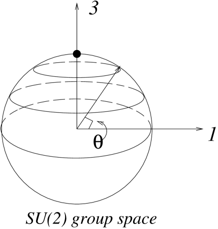
Figure 2: Unwinding the ANO ansatz.

It is not difficult to devise an ansatz encoding the possibility of unwinding the field configuration (3.1) through the loop shrinkage in the SU(2) group space. The ansatz which does the job and eventually will allow us to calculate the ANO string decay rate is parametrized by an angle parameter $\theta$,

$$q_{k}(x) = U\,e_{k}\,q_{\theta}(r)\,,\qquad(e_{1}=1,\;e_{2}=0)\,,$$

$$A_{0} \equiv 0\,,\qquad A_{3}\equiv 0\,,$$

$$A_{j}(x) = i\,U\partial_{j}\,U^{-1}\,[1-f_{\theta}(r)]\,,\qquad j=1,2\,,$$

$$\phi = V\,U\,\frac{\tau_{3}}{2}\,U^{-1}+\Delta\phi\,,$$ (4.1)

where

$$U=e^{-i\alpha\tau_{3}}\cos{\theta}+i\,\tau_{1}\,\sin{\theta}\,.$$ (4.2)

(Eventually, upon quantization, $\theta$ will become a slowly varying function of $z$ and $t$, a field $\theta(t,z)$.)

The gauge and quark fields in (4.1) are parametrized by profile functions $f_{\theta}(r)$ and $q_{\theta}(r)$ depending on the parameter $\theta$. They satisfy the same boundary conditions

$$q_{\theta}(0)=0\ ,\qquad~{}f_{\theta}(0)=1,$$

$$q_{\theta}(\infty)=v\ ,\quad f_{\theta}(\infty)=0\$$ (4.3)

as in the U(1) case, see Eq. (3.3). The boundary conditions at zero are chosen to ensure the absence of singularities of our ansatz at $r=0$. The magnetic flux of the string (4.1) is

$$2\pi\cos^{2}{\theta}.$$ (4.4)

It equals to $2\pi$ at $\theta=0$ and goes to zero at $\theta=\frac{\pi}{2}$.

The term $\Delta\phi$ in the last line of Eq. (4.1) is needed to make sure that there is no singularity at $r\to 0$. For axially symmetric string the function $\Delta\phi$ can be chosen in the form

$$\Delta\phi=\varphi_{\theta}(r)\,\left[\frac{\tau_{1}}{2}\,\sin{\alpha}-\frac{\tau_{2}}{2}\,\cos{\alpha}\right]\,,$$ (4.5)

where we assume that the component of $\Delta\phi$ along $\tau_{3}$ is zero, while $\varphi_{\theta}(r)$ is an extra profile function, which depends on $\theta$ as a parameter. The $a=1,2$ components of $\Delta\phi$ cannot be put to zero. To see this substitute Eqs. (4.2) and (4.5) into the last line in Eq. (4.1). Then one gets

$$\phi=\frac{\tau_{3}}{2}\,V\,\cos{2\theta}-\left[\frac{\tau_{1}}{2}\,\sin{\alpha}-\frac{\tau_{2}}{2}\,\cos{\alpha}\right]\,\left[V\sin{2\theta}-\varphi_{\theta}(r)\right]\,.$$ (4.6)

From this expression it is clear that $\phi$ has no singularity at $r=0$ provided that

$$\varphi_{\theta}(0)=V\sin{2\theta}\,.$$ (4.7)

The boundary condition for $\varphi_{\theta}(r)$ at infinity should be chosen as follows:

$$\varphi_{\theta}(\infty)=0\,.$$ (4.8)

Both boundary conditions are consistent with the initial condition

$$\left.\varphi_{\theta}(r)\right|_{\theta=0}=0\,,$$ (4.9)

to be imposed.

For future reference it is convenient to present the very same ansatz (4.1) in the singular gauge,

$$q_{k}(x) = e_{k}\,q_{\theta}(r)\,,$$

$$A_{i}(x) = -i\,(\partial_{i}U^{-1})\,U\,f_{\theta}(r)\,,$$

$$\phi = V\,\frac{\tau_{3}}{2}\,+U^{-1}\,(\Delta\phi)\,U\,.$$ (4.10)

Our ansatz, Eqs. (4.1) or (4.10), plus (4.2), smoothly interpolates between the ANO-type winding along the equator at $\theta=0$, and constant matrix with no winding at $\theta={\pi}/{2}$. In other words, we start from the ANO string at $\theta=0$ and arrive at empty vacuum at $\theta=\pi/2$. Indeed, at $\theta=0$ the adjoint field $\phi$ is aligned, $\phi^{a}=V\delta^{3a}$, while $U=e^{-i\alpha\tau_{3}}$. At $\theta={\pi}/{2}$ again $\phi^{a}=V\delta^{3a}$, and $U=i\tau_{1}$, implying $A_{j}=0$. (Equivalently, one could have chosen to end up with $U=i\tau_{2}$ at $\theta=\frac{\pi}{2}$.) Thus, we managed to unwind the ANO winding through extra dimension of the vacuum manifold in the SU(2) theory which was not there in QED.

We pause here to make an additional comment regarding our ansatz (4.1). At large $r$, when $q_{\theta}\to v$ and $f_{\theta}\to 0$ and $\varphi_{\theta}\to 0$, our field configuration presents a gauge-transformed “plain vacuum”. This ensures that at every given $\theta$ the energy functional converges at large $r$. The convergence of the energy functional at small $r$ is guaranteed by the boundary conditions $q_{\theta}(0)=0\,,\,\,\,f_{\theta}(0)=1$ and (4.7).

The tension of the string (or the field configuration in which it evolves at $\theta\neq 0$) is a functional of three functions $f_{\theta}(r)$ , $q_{\theta}(r)$ and $\varphi_{\theta}(r)$. It is easy to get this functional by substituting the ansatz (4.1) in the action (2.1). Restricting ourselves to (1,2)-plane we obtain after some algebra

$$T(\theta) = \!\!\!2\pi\int rdr\,\left\{\frac{2}{g^{2}}\,\frac{f_{\theta}^{\prime 2}}{r^{2}}\,\cos^{2}{\theta}+q_{\theta}^{\prime 2}+\frac{f_{\theta}^{2}}{r^{2}}\,q_{\theta}^{2}\,\cos^{2}{\theta}\right.$$ (4.11)

$$+ \!\!\!\frac{1}{2}\varphi_{\theta}^{\prime 2}+\frac{1}{2r^{2}}\left[\varphi_{\theta}(\cos{2\theta}-2f_{\theta}\cos^{2}{\theta})+Vf_{\theta}\sin{2\theta}\right]^{2}$$

$$+ \!\!\!\left.\lambda(q_{\theta}^{2}-v^{2})^{2}+\tilde{\lambda}\left[\varphi_{\theta}^{2}-2V\varphi_{\theta}\sin{2\theta}\right]^{2}+\frac{\gamma}{4}\varphi_{\theta}^{2}q_{\theta}^{2}\right\}\,.$$

Needless to say that at $\theta=0$ the string tension $T$ coincides with that for the ANO string, see (3.4), while at $\theta={\pi}/{2}$ it goes to zero, as was expected.

Now we have to minimize the string functional (4.11) with respect to three profile functions $f_{\theta}(r)$ , $q_{\theta}(r)$ and $\varphi_{\theta}(r)$ at fixed $\theta$. This procedure would give us a solution for the profile functions. Finding the full solution is a rather complicated task requiring numerical computations which go beyond the scope of the present paper. However, we will be able to get sufficient insight in order to derive the general formula (1.3) by purely analytical means.

Why we call the ansatz (4.1) primitive? It has only one profile function $f_{\theta}(r)$ for all three gauge components. This is okay at $\theta=0$ when the $W$ boson degrees of freedom are not excited. At $\theta\neq 0$ the universality of $f_{\theta}(r)$ forces one and the same spread in the perpendicular plane of the $W$ boson and photon components of the solution. As a result, unwinding of the ANO strings in Eq. (4.1) proceeds via the production of highly excited “monopoles.” This shortcoming can be eliminated through introduction of extra profile functions, see Sect. 8 and Appendix.

5 Extreme type II string

As we have already mentioned, even for the stable ANO string the analytic solution for generic values of the ratio $m_{q}/m_{\gamma}$ is absent. On the other hand, it is not difficult to find the solution that would be valid in the logarithmic approximation, $\ln m_{q}/m_{\gamma}\gg 1$. Therefore, in this section we consider the extreme type II superconductor for which we will be able to obtain an analytic solution of the problem of the decaying string.

In fact, we impose the following relation between the adjoint scalar, quark and photon masses:

$$m_{a}\gg m_{q}\gg m_{\gamma}.$$ (5.1)

In addition, it is convenient to limit ourselves to the case $m_{W}\sim m_{a}$. At first, we review Abrikosov’s solution for the ANO string [3], then consider the decaying string and, finally, work out the effective action for the unstable mode on the string world-sheet and calculate the string decay rate.

5.1 Type II ANO string

Assume that $m_{q}\gg m_{\gamma}$ in the Abelian Higgs model (2.7). Then the ANO string looks as follows. The quark field $q(r)$ varies from zero to its vacuum value $v$ inside a small core of radius of order of $1/m_{q}$, whereas the electromagnetic field is spread over a much larger domain, of order of $1/m_{\gamma}$. In the latter domain the quark field is already very close to its VEV. The solution of the second equation in (3.2) for the gauge profile function $f$ is $f\sim r^{2}$ in this domain (where the last term in this equation can be ignored). Being properly normalized, the solution has the following asymptotics:

$$f=\left\{\begin{array}[]{l}1-c\,m_{\gamma}^{2}\,r^{2}\quad\mbox{at}\quad r\ll m_{\gamma}^{-1}\,,\\[8.53581pt] 0\quad\mbox{at}\quad r\gg m_{\gamma}^{-1}\,,\end{array}\right.$$ (5.2)

where $c$ is a constant, $c\sim 1$. The approach to zero at $r\gg m_{\gamma}^{-1}$ is exponentially fast.

The leading (and the only) logarithmic contribution to the string tension comes from the third term in the expression (3.4) for the ANO string tension. In the domain $m_{q}^{-1}\ll r\ll m_{\gamma}^{-1}$, with the logarithmic accuracy, one can substitute in Eq. (3.4) $q=v$ and retain only the leading term in the gauge profile function, $f=1+\cdots$. In this way one gets

$$T_{\rm ANO}^{\rm II}=2\pi v^{2}\,\ln\,\frac{m_{q}}{m_{\gamma}}\,.$$ (5.3)

Domains other than $m_{q}^{-1}\ll r\ll m_{\gamma}^{-1}$ yield a non-logarithmic contribution. The same is valid with regards to the first, second and fourth terms in Eq. (3.4), as well as deviations from $q=v$ and $f=1$. All these effects give corrections to (5.3) suppressed by powers of $1/\ln(m_{q}/m_{\gamma})$.

This result was obtained by Abrikosov in 1957 [3]. Note that the leading logarithmic contribution to the string tension (5.3) is totally insensitive to details of the profile functions $q$ and $f$. It “feels” only the boundary values $q(\infty)=v$ and $f(0)=1$.

5.2 Decaying type II string

Now we use the same method of separating distinct physical scales to describe the decaying extreme type II string. Our goal is calculating the barrier (potential energy versus $\theta$) which will be later used in the calculation of the decay rate. We will need the kinetic term for the field $\theta(t,z)$ too, but we begin with the potential term.

The condition (5.1) ensures that both, the adjoint scalar and quark fields vary in small cores with sizes of order $1/m_{a}$ and $1/m_{q}$, respectively. In the domain $m_{q}^{-1}\ll r\ll m_{\gamma}^{-1}$ the fields $\phi$ and $q$ already reach their boundary values $\varphi_{\theta}(\infty)=0$ and $q_{\theta}(\infty)=v$. Moreover, we again use Eq. (5.2) for the function $f_{\theta}$, the leading logarithmic contribution to the tension coming from the boundary value $f_{\theta}(0)=1$.

Substituting this data in Eq. (4.11) we get

$$T^{\rm II}(\theta)=2\pi\,\left(\ln\,\frac{m_{q}}{m_{\gamma}}\right)\,v^{2}\,\cos^{2}{\theta}+2\pi\,\left(\ln\,\frac{m_{a}}{m_{\gamma}}\right)\,\frac{V^{2}}{2}\,\sin^{2}{2\theta}\,.$$ (5.4)

This is our result for the barrier profile for the extreme type II string. The first term here comes from the third term in Eq. (4.11) while the second one comes from the fifth term in Eq. (4.11). All other contributions to $T$ contain no large logarithms. At $\theta=0$ the tension in (5.4) coincides with that of the ANO string, see Eq. (5.3). At non-zero $\theta$ the $V^{2}$ term dominates — it produce a huge barrier, with the height of order of $V^{2}\,\ln\,(m_{a}/m_{\gamma})$. At $\theta={\pi}/{2}$ the tension $T^{\rm II}(\theta)$ vanishes, which means that the string disappears. This is summarized in Fig. 3 presenting $T^{\rm II}(\theta)$ versus $\theta$.

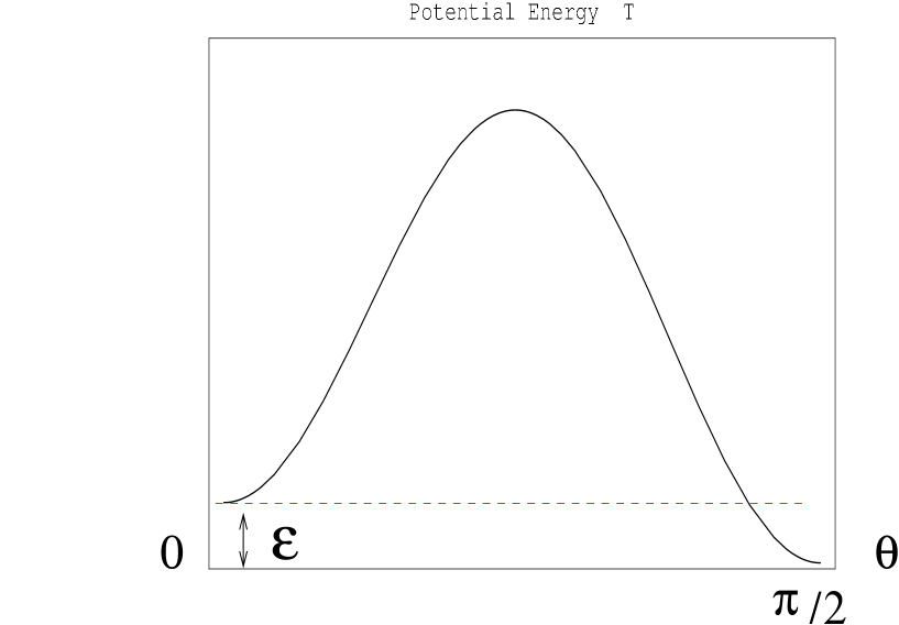
Figure 3: The potential energy $T(\theta)$.

5.3 Effective world-sheet theory

In order to calculate the decay rate of the string we have to work out the effective theory for the unstable mode parametrized by $\theta$ on the string world-sheet. The collective coordinate $\theta$ becomes a field of a 2D sigma model on the string world-sheet. The tension (5.4) gives us the potential term in the action of this sigma model. To complete the problem we need to know the kinetic term.

In order to obtain the kinetic term we apply the standard strategy: we assume that $\theta$ adiabatically depends on the world-sheet coordinates $\sigma$. (Throughout the paper we use here the static gauge for the string in which $\sigma_{1}=t$ and $\sigma_{2}=x_{3}$.) The kinetic term for $\theta$ in the 2D sigma model comes from those in the action (2.1). To calculate the kinetic term for $\theta$ it is convenient to rotate our field configuration (4.1) into a “singular” gauge performing the gauge transformation with the matrix $U^{-1}$, see Eq. (4.10). In this gauge the boundary values of the fields at infinity do not depend on $\theta$ and give no contribution to the kinetic energy term, for instance, $q_{k}(x)=e_{k}\,q_{\theta}(r)$, and

$$\phi=V\,\frac{\tau_{3}}{2}\,+U^{-1}\,(\Delta\phi)\,U\,,$$ (5.5)

(remember, $\Delta\phi$ falls off at infinity). The gauge field falls off rapidly at large distances,

$$A_{i}(x) =-i\,(\partial_{i}U^{-1})\,U\,f_{\theta}(r)\,.$$ (5.6)

We pause here to discuss a subtle point in the calculation of the kinetic term. With time dependence switched off, for the static string, the non-vanishing components of the gauge potential are $A_{j}$, ($j=1,2$). The components $A_{n}$ with $n=0,3$ vanish, see Eq. (4.1). However, as soon as we allow $\theta$ to depend on the world-sheet coordinates, the components $A_{n}$ with $n=0,3$ must become non-zero. Indeed, let us first assume that $A_{n}=0$ (we will immediately see that this is a wrong assumption). Consider the contribution of the kinetic term of the gauge field $F_{\mu\nu}^{2}$. It is clear that the only $F_{nj}^{2}$ piece contributes to the kinetic term of $\theta$,

$$F_{n\,j}=\partial_{n}A_{j}-\partial_{j}A_{n}-i\,[A_{n}\,,A_{j}]\,,\quad j=1,2\,,\quad n=0,3\,.$$ (5.7)

If the components $A_{n}$ vanished, then one would obtain

$$F_{n\,j}=\partial_{n}\,A_{j}=(\partial_{n}\theta)\,(\partial_{\theta}A_{j})\,,$$ (5.8)

which, being combined with Eq. (5.5) for the gauge potential $A_{j}$, yields

$$\partial_{n}A_{j}=2\,(\partial_{n}\theta)\,\varepsilon_{j\ell}\,\frac{x_{\ell}}{r^{2}}\,\left[\sin{2\theta}\,\,\frac{\tau_{3}}{2}+\cos{2\theta}\left(\frac{\tau_{1}}{2}\sin{\alpha}+\frac{\tau_{2}}{2}\cos{\alpha}\right)\right]f_{\theta}(r)\,.$$ (5.9)

With this formula the expression for $F_{nj}^{2}$ is not even gauge invariant with respect to the gauge transformations depending on $\theta$, see Eq. (5.8).

The fact that we made a mistake by assuming $A_{n}=0$ manifests itself in the singularity in Eq. (5.9) at $r=0$ (note that $f_{\theta}(0)=1$, see Eq. (4.3)).

Thus, in the calculation of the kinetic term of $\theta$ one cannot avoid switching on the components $A_{n}$ with $n=0,3$ which, naturally, must be proportional to $\partial_{n}\theta$. The following ansatz for $A_{n}$ goes through:

$$A_{n}=-2\,(\partial_{n}\theta)\left(\frac{\tau_{1}}{2}\,\cos{\alpha}-\frac{\tau_{2}}{2}\,\sin{\alpha}\right)a_{\theta}(r)\,,$$ (5.10)

where $a_{\theta}(r)$ is a new profile function and the angle $\alpha$ is defined in Fig. 1. Generally speaking, $A_{n}$ is parametrized by three distinct profile function accounting for three generators of SU(2). However, as it turns out, the single structure presented in Eq. (5.10), leads to a fully self-consistent and complete ansatz, with the $r\to 0$ singularity in $F_{nj}$ cancelled. We do not need two other structures.

Substituting Eq. (5.10) in Eq. (5.7) and ignoring terms that are a priori non-singular at $r=0$, we get

$$F_{n\,j}=2\,(\partial_{n}\theta)\,\varepsilon_{j\ell}\,\frac{x_{\ell}}{r^{2}}\,\left[\sin{2\theta}\,\frac{\tau_{3}}{2}+\cos{2\theta}\left(\frac{\tau_{1}}{2}\sin{\alpha}+\frac{\tau_{2}}{2}\cos{\alpha}\right)\right]\left(1-a_{\theta}(r)\right)\,,$$ (5.11)

where we assume that the gauge profile function $f_{\theta}=1+\cdots$ at $r\ll 1/m_{\gamma}$. The reason why we can keep only the most singular terms is as follows. Let us remind that in Sect. 5.2 we found the potential term for the $\theta$ field in the logarithmic approximation (i.e. the approximation in which only those terms are kept which contain large logarithms of the mass ratio). Our task in this section is to find the kinetic term for the $\theta$ field in the very same logarithmic approximation.

In order to cancel the actual divergence of $\int d^{2}x\,F_{n\,j}^{2}$ at $r\to 0$ we must impose the following boundary condition:

$$a_{\theta}(0)=1\,,$$ (5.12)

as well as

$$a_{\theta}(\infty)=0\,.$$ (5.13)

In fact, for our purposes — determination of the kinetic term with the logarithmic accuracy — it is sufficient to use the step function model for $a_{\theta}(r)$ similar to that in Eq. (5.2),

$$a_{\theta}(r)=\left\{\begin{array}[]{l}1\quad\mbox{at}\quad r\ll R\,,\\[8.53581pt] 0\quad\mbox{at}\quad r\gg R\,,\end{array}\right.$$ (5.14)

where we introduced a new parameter $R$, to be determined below, (it is assumed that $R\ll 1/m_{\gamma}$).

With the profile function $a_{\theta}(r)$ presented in Eq. (5.14), the contribution of the gauge term to the kinetic energy of the field $\theta$ takes the form

$$\int d^{2}x\,\frac{1}{4g^{2}}\,F_{\mu\nu}^{a}F^{\mu\nu\,\,a}\rightarrow\frac{4\,\pi}{g^{2}}\,(\partial_{n}\theta)^{2}\,\ln{\frac{1}{Rm_{\gamma}}}\,.$$ (5.15)

This is not the end of the story, however, since, in addition, we have to take into account the kinetic energy coming from the scalar kinetic terms in Eq. (2.1) (the second and the third terms). It is obvious that the third term, associated with the quark field, is proportional to $v^{2}$ and can be neglected as compared to the second term — the contribution of the adjoint scalar which is proportional to $V^{2}$. As a result, using Eq. (5.10) to calculate $D_{n}\phi$, we get for the total kinetic energy

$$4\pi\,(\partial_{n}\,\theta)^{2}\left[\frac{1}{g^{2}}\ln{\frac{1}{R\,m_{\gamma}}}+{\rm const}\cdot(V^{2}\,R^{2})\right]\,.$$ (5.16)

The parameter $R$ can now be determined from the requirement that the coefficient in front of $(\partial_{n}\theta)^{2}$ be minimal. Minimizing this with respect to $R$ we find the condition

$$\frac{1}{g^{2}\,R}\sim V^{2}\,R\,.$$

In other words, $R$ turns out to be small, of the order of the inverse mass of the W boson,

$$R\sim\frac{1}{m_{W}}\,,$$ (5.17)

in full accord with what our physical intuition demands. With this value of the parameter $R$, the first logarithmic term in Eq. (5.16) dominates over the second one, which can be thus ignored with the logarithmic accuracy. As a result, combining together the kinetic term (5.16) with the potential term (5.4), we arrive at the following action of the 2D sigma model:

$$S_{\rm str\,\,II} = 2\pi\,\int d^{2}\sigma\,\left\{\frac{2}{g^{2}}\left(\ln{\frac{m_{W}}{m_{\gamma}}}\right)\,(\partial_{n}\theta)^{2}\right.$$ (5.18)

$$- \left.\!\!\!\!\left(\ln{\frac{m_{q}}{m_{\gamma}}}\right)\,v^{2}\cos^{2}{\theta}-\left(\ln{\frac{m_{a}}{m_{\gamma}}}\right)\,\frac{V^{2}}{2}\sin^{2}{2\theta}\right\}\,.$$

This is our final result for the effective theory of the unstable $\theta$-mode on the string world-sheet in the primitive ansatz. In what follows we will assume that the masses $m_{W}$ and $m_{a}$ are of the same order of magnitude, i.e. $\tilde{\lambda}\sim g^{2}$. In the logarithmic approximation we can then replace the logarithms in the first and the third terms in Eq. (5.18) by a single logarithm, say ln$\,m_{W}/m_{\gamma}$. This assumption is by no means crucial.

5.4 Decays through tunneling (“bubbles of true vacua”)

To calculate the decay rate of the metastable string we may forget for a while about the microscopic theory (2.1) and turn our attention to the effective theory (5.18). In this latter theory the string state is nothing but “the false vacuum state” at $\theta\approx 0$, see Fig. 3, while the “no-string state” is the true vacuum at $\theta\approx\pi/2$.

The metastable string decay occurs through the creation of the monopole-like objects: at a certain $z=-z_{0}$ a magnetic charge is produced, accompanied by the production of an anticharge at $z=z_{0}$, through tunneling. In the interval $-z_{0}<z<z_{0}$ the magnetic flux tube is eliminated.

The corresponding process in the effective theory looks as follows. In the initial moment of time the theory resides in the false vacuum. Then it tunnels into the true one. The tunneling creates an interval of true vacuum, which subsequently experiences an unlimited classical expansion.

The quantitative description of the false vacuum decay is well-developed within the quasiclassical approximation [24, 25], which is fully applicable to the 2D sigma model (5.18). The applicability of the quasiclassical approximation will become clear shortly. The parameter which regulates this approximation is $V/v\gg 1$.

Let us briefly review the general procedure [24, 25] of calculating the probability of the false vacuum decay (for a comprehensive review see [31]). Details (as well as the final answer) slightly depend on the space-time dimension. Since our effective world-sheet theory (5.18) is (1+1)-dimensional, we will focus on this case.

An appropriate description of the tunneling probability implies a Euclidean rotation,

$$t\to i\,t\,.$$

After the Euclidean rotation, the Euclidean action of the effective world-sheet theory takes the form

$$S_{\rm Eucl}=2\pi\,\left(\ln{\frac{m_{W}}{m_{\gamma}}}\right)\!\!\!\!\!\!\!\!\!\! \int d^{2}\sigma\,\left\{\frac{2}{g^{2}}\left[(\dot{\theta})^{2}+(\partial_{z}\theta)^{2}\right]+\frac{V^{2}}{2}\sin^{2}{2\theta}\right.$$ (5.19)

$$+ \left.\kappa\,v^{2}\cos^{2}{\theta}\right\}\,,$$

$$\kappa \equiv \left(\ln{\frac{m_{q}}{m_{\gamma}}}\right)\left(\ln{\frac{m_{W}}{m_{\gamma}}}\right)^{-1}\,.$$ (5.20)

In this formulation the false vacuum decay goes through the creation of a bubble of the true vacuum inside the false one, see Fig. 4. The bubble is a classical bounce solution in the potential $V(\theta)=-T^{\,\rm II}(\theta)$ which depends only on the radial variable $\sqrt{t^{2}+z^{2}}$. In the thin wall approximation which is relevant to our problem the concrete form of the bounce solution in the model (5.19) is not important. The only parameter we will need to know is the tension $\tau$ of the bubble surface.

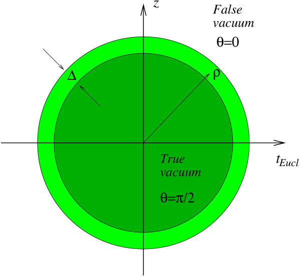
Figure 4: False vacuum decay through a bubble of true vacuum (in the Euclidean time).

The bounce solution has a negative mode associated with instability in the bubble size $\rho$. Integration over this negative mode produces an imaginary part of the vacuum energy. The latter determines the false vacuum decay rate [24, 25] which thus is proportional to

$$\Gamma\sim\exp{\left(-S_{\rm bubble}\right)},$$ (5.21)

where $S_{\rm bubble}$ is the classical action of the bounce.

In the problem at hand the ratio of the critical size of the bubble to the bubble surface thickness is very large (it is regulated by the same parameter $V/v\gg 1$). Therefore, to calculate the bubble surface tension $\tau$ one can neglect its curvature and consider a flat wall separating two vacua — one at $\theta\approx 0$ and another at $\theta\approx\pi/2$. Simultaneously we can (and should) neglect the term $\kappa\,v^{2}\cos^{2}{\theta}$ in Eq. (5.19) which is responsible for the non-degeneracy of these two vacua. With the term $\kappa\,v^{2}\cos^{2}{\theta}$ switched off, the vacua at $\theta\approx 0$ and $\theta\approx\pi/2$ become degenerate, and the flat wall perfectly stable.

The tension of the flat wall is obtained from minimization of the energy functional

$$\tau=4\pi\left(\ln\frac{m_{W}}{m_{\gamma}}\right)\,\int\,dz\left\{\frac{1}{g^{2}}\,\left(\partial_{z}\,\theta\right)^{2}+\frac{V^{2}}{4}\,\sin^{2}{2\theta}\right\}\,,$$ (5.22)

with the boundary conditions

$$\theta=0\,\,\,\mbox{at}\,\,\,z\to-\infty\,,\qquad\theta=\frac{\pi}{2}\,\,\,\mbox{at}\,\,\,z\to\infty\,.$$ (5.23)

The solution of the minimization condition is a well-known sine-Gordon soliton,

$$\theta(z)=\frac{1}{2}\,\left\{{\rm arcsin}\left({\rm tanh}\,m_{W}z\right)+\frac{\pi}{2}\right\}\,.$$ (5.24)

The mass of the sine-Gordon kink gives the wall tension $\tau$,

$$\tau=4\,\pi\,\left(\ln\frac{m_{W}}{m_{\gamma}}\right)\,\frac{V}{g}\,.$$ (5.25)

The wall thickness is inversely proportional to the $W$ boson mass,

$$\Delta\sim m_{W}^{-1}\,.$$ (5.26)

The potential term in Eq. (5.19) presents a huge barrier under which the false vacuum must tunnel. At the same time, the energy density difference between the false and true vacua — we denote it by ${\cal E}$ — is small since it is determined by the third term in Eq. (5.19),

$${\cal E}\equiv T_{\rm ANO}^{\,\rm II}=2\pi\,v^{2}\,\ln\,\left(\frac{m_{q}}{m_{\gamma}}\right)\,.$$ (5.27)

The action of the bubble on the tunneling trajectory is given by [24]

$$S_{\rm bubble}=2\pi\rho\,\tau-\pi\rho^{2}{\cal E}\,.$$ (5.28)

The size of the critical bubble $\rho_{*}$ is determined by the extremum of the action,

$$\rho_{*}=\frac{\tau}{{\cal E}}=2\left(\frac{V}{v}\right)^{2}\frac{1}{gV\,\kappa}\,.$$ (5.29)

The ratio of the bubble radius to the wall thickness is indeed very large,

$$\frac{\rho_{*}}{\Delta}\sim\left(\frac{V}{v}\right)^{2}\gg 1\,,$$ (5.30)

which justifies the thin wall approximation.

Substituting the critical size from Eq. (5.29) in Eq. (5.28) we find the tunneling action, $S_{*}=\pi{\tau^{2}}/{{\cal E}}$. The probability of the false vacuum decay which is equal to the probability (per unit time per unit length) of the ANO string breaking is

$$\Gamma_{\rm breaking}^{\,\rm II} \sim e^{-S_{*}}=\exp\left(-\pi\,\frac{\tau^{2}}{{\cal E}}\right)$$ (5.31)

$$= \exp\left\{-\frac{8\pi^{2}}{g^{2}}\,\,\frac{V^{2}}{\kappa\,v^{2}}\,\left(\ln\,\frac{m_{W}}{m_{\gamma}}\right)\right\}\,,$$

where the parameter $\kappa$ is defined in Eq. (5.20). We conclude this section by rewriting Eq. (5.31) in terms of the ANO string tension (5.3),

$$\Gamma_{\rm breaking}^{\,\rm II}\sim\exp\left\{-\,\frac{16\pi^{3}}{g^{2}}\left(\ln\,\frac{m_{W}}{m_{\gamma}}\right)^{2}\,\frac{V^{2}}{T_{\rm ANO}^{\,\rm II}}\right\}\,.$$ (5.32)

We will see in Sect. 6 that the decay rate of extreme type I string, being expressed in terms of the type I string tension, is given by the very same formula.

6 Extreme type I string

In this section we will consider strings in the limit of very small quark masses. We still assume that the adjoint scalar mass is much larger than all other scales, in other words we impose the condition

$$m_{W}\sim m_{a}\gg m_{\gamma}\gg m_{q}\,.$$ (6.1)

We will begin with a brief review of the stable ANO strings in this case, and then turn to decaying strings. To avoid bulky expressions in what follows it will be convenient to introduce a parameter $L$,

$$L=\ln\frac{m_{\gamma}}{m_{q}}\,,$$ (6.2)

and a function $L(\theta)$,

$$L(\theta)=\ln\,\frac{m_{\gamma}}{m_{q}\cos\theta}\,.$$ (6.3)

6.1 Type I ANO string

Let us outline the solution [15] for the ANO string in the Abelian Higgs model (2.7) under the condition $m_{\gamma}\gg m_{q}$.

To the leading order in $L=\ln\,(m_{\gamma}/m_{q})$ the vortex solution has the following structure. The electromagnetic field is confined to a core with the radius $R_{g}$ which we will estimate momentarily. The profile function for the gauge field is given, approximately, by an expression similar to Eq. (5.2),

$$f=\left\{\begin{array}[]{l}1-\frac{r^{2}}{R_{g}^{2}}\,,\quad r\ll R_{g}\,,\\[8.53581pt] 0,\qquad\,\,\,\,\,\,\,\,r\gg R_{g}\,.\end{array}\right.$$ (6.4)

Moreover, the quark field is close to zero inside this core. On the other hand, outside the core, the electromagnetic field is vanishingly small. At intermediate distances

$$R_{g}\ \ll\ r\ \ll\ \frac{1}{m_{q}}$$ (6.5)

the scalar field satisfies the free equation of motion, see the first equation in (3.2), where the third and the last terms can be ignored. Its solution is as follows:

$$q(r)=v\left\{1-\left(\ln\,\frac{1}{rm_{q}}\right)\left(\ln\,\frac{1}{R_{g}m_{q}}\right)^{-1}\right\}\,.$$ (6.6)

At large distances, $r\gg 1/m_{q}$, the function $q(r)$ approaches its VEV $v$, the rate of approach is exponential,

$$q\to v\left(1+C\,\exp(-m_{q}r)\right)\,.$$

Now, substituting Eqs. (6.4) and (6.6) in Eq. (3.4) we get the tension of the static type I string as a function of $R_{g}$,

$$T_{\rm ANO}^{\,\rm I}\ =\ 2\pi\,\left[\frac{\rm const}{g^{2}\,R^{2}_{g}}\,+\,{v^{2}}\,\left(\ln\,\frac{1}{R_{g}m_{q}}\right)^{-1}\right]\,.$$ (6.7)

The first term here comes from the first term in Eq. (3.4)) which is concentrated inside the core. The second term in Eq. (6.7) comes from the logarithmically large region (6.5), where the quark field is given by Eq. (6.6).

Minimizing the right-hand side of Eq. (6.7) with respect to $R_{g}$ we determine $R_{g}$,

$$R^{2}_{g}\ \sim\ \frac{1}{m^{2}_{\gamma}}\,L^{2}=\frac{1}{m^{2}_{\gamma}}\left(\ln\frac{m_{\gamma}}{m_{q}}\right)^{2}\,.$$ (6.8)

This expression demonstrates that in the case at hand the size of the string core is logarithmically larger than $1/m_{\gamma}$, due to the presence of the light scalar $q$.

Using this result for $R_{g}$ it is straightforward to evaluate the tension of the extreme type I string. To this end we plug Eq. (6.8) back in Eq. (6.7) and then obtain [15]

$$T_{\rm ANO}^{\,\rm I}\ =\ {2\pi v^{2}}\,L^{-1}\,,$$ (6.9)

where $L$ is defined in Eq. (6.2). The tension $T_{\rm ANO}^{\,\rm I}$ is saturated, in the logarithmic approximation, by the kinetic energy of the quark field (the second term in Eq. (3.4), the “surface” energy). All other terms in Eq. (3.4), as well as corrections to profile functions, yield contributions suppressed by extra powers of $L^{-1}$.

6.2 Decaying type I string

We now turn to the derivation of an effective 2D world-sheet theory for the unstable mode $\theta(t,z)$ for the extreme type I strings. Our first task is determination of the potential term.

The description of the decaying type I string we are going to use runs parallel to that for type II, see Sects. 4 and 5. The adjoint scalar $\varphi_{\theta}$ varies from its boundary value (4.7) to zero in a very narrow core whose size is of the order of $1/m_{a}$. The profile function $f_{\theta}$ for the electromagnetic field is concentrated inside a larger core, of radius $R_{g}(\theta)$. Note that the parameter $R_{g}$ introduced above now becomes a $\theta$ dependent function. Inside this “electromagnetic” core the profile function $f_{\theta}$ is approximately given by Eq. (6.4) with $R_{g}$ replaced by $R_{g}(\theta)$. The quark field is very small inside this core, while outside it is given by Eq. (6.6), again with the replacement $R_{g}\to R_{g}(\theta)$. Assembling all these elements together and substituting in Eq. (4.11) we get

$$T^{\rm I}(\theta)=2\pi\,\left[{\rm const}\,\,\frac{\cos^{2}{\theta}}{g^{2}(R_{g}(\theta))^{2}}\,+\,{v^{2}}\,\left(\ln\,\frac{1}{R_{g}m_{q}}\right)^{-1}\,+\left(\ln\,\frac{m_{a}}{m_{\gamma}}\right)\,\frac{V^{2}}{2}\sin^{2}{2\theta}\right]\,.$$ (6.10)

Next, for each given $\theta$ one determines $R_{g}(\theta)$ by minimizing $T^{\rm I}(\theta)$ with respect to $R_{g}$. In this way one finds

$$R_{g}(\theta)\ \sim\ \frac{\cos{\theta}}{m_{\gamma}}\,L\,,$$ (6.11)

(cf. Eq. (6.8)). With this expression for $R_{g}(\theta)$ the tension of the decaying type I string versus $\theta$ (in the logarithmic approximation) takes the form

$$T^{\rm I}(\theta)=\frac{2\pi\,v^{2}}{L(\theta)}+2\pi\,\left(\ln\,\frac{m_{a}}{m_{\gamma}}\right)\,\frac{V^{2}}{2}\sin^{2}{2\theta}\,,$$ (6.12)

where the function $L(\theta)$ is defined in Eq. (6.3). The boundary values are as follows. At $\theta=0$ the potential term $T^{\,\rm I}(\theta)$ is equal to the static string tension (6.9). At larger $\theta$ the potential $T^{\rm I}(\theta)$ develops a very high barrier (at the maximum $T^{\,\rm I}(\theta)\sim V^{2}\,\ln\,(m_{a}/m_{\gamma})$), and then it vanishes at $\theta=\pi/2$. Qualitatively, the behavior of $T^{\,\rm I}(\theta)$ is perfectly the same as that depicted in Fig. 3. Equation (6.12) concludes our calculation of the potential term in the effective world-sheet action for the $\theta$-mode of the type I string.

Calculation of the kinetic term for the type I string repeats the same steps we made in Sect. 5.3 for type II and thus gives the same result for the kinetic term of type I as in Eq. (5.18). It is easy to understand why: the solution for the gauge field is essentially the same for the two cases. Assembling together the kinetic and potential terms we finally arrive at the following effective world-sheet theory for the unstable mode of the extreme type I string:

$$S_{\rm str\,\,I}=2\pi\,\int d^{2}\sigma\,\left\{\frac{2}{g^{2}}\left(\ln{\frac{m_{W}}{m_{\gamma}}}\right)\,(\partial_{n}\theta)^{2}-\frac{v^{2}}{L(\theta)}-\left(\ln{\frac{m_{a}}{m_{\gamma}}}\right)\,\frac{V^{2}}{2}\sin^{2}{2\theta}\right\}\,.$$ (6.13)

We are now ready to consider the false vacuum decay in this sigma model. As in Sect. 5.4, the decay rate is given by the formula

$$\Gamma\sim\exp\left(-\pi\,\frac{\tau^{2}}{{\cal E}}\right)\,,$$ (6.14)

where ${\cal E}$ is the difference between the energy densities in the false and true vacua, ${\cal E}=T_{\rm ANO}^{\,\rm I}$, see Eq. (6.9), while $\tau$ is the tension of the flat wall separating the two vacua. Remember, to calculate the latter we neglect the term $v^{2}/L(\theta)$ in the potential energy. Hence, the wall solution, as well as $\tau$, are exactly the same as in Sect. 5.4, see Eq. (5.25), provided that $m_{a}\sim m_{W}$, so that the logarithms of $m_{W}/m_{\gamma}$ and $m_{a}/m_{\gamma}$ are the same. We accept this simplifying assumption.

Substituting $\tau$ and ${\cal E}$ in Eq. (6.14) we finally arrive at the decay rate (per unit length) of the extreme type I string,

$$\Gamma^{\,\rm I}_{\rm breaking}\sim\exp\left\{-\frac{8\pi^{2}}{g^{2}}\,\frac{V^{2}}{v^{2}}\,\left(\ln\,\frac{m_{W}}{m_{\gamma}}\right)^{2}\,\left(\ln\,\frac{m_{q}}{m_{\gamma}}\right)\right\}\,.$$ (6.15)

Needless to say that if we express this decay rate in terms of the type I string tension we get the same formula (5.32) as for the type II string,

$$\Gamma_{\rm breaking}^{\,\rm I}\sim\exp\left\{-\,\frac{16\pi^{3}}{g^{2}}\left(\ln\,\frac{m_{W}}{m_{\gamma}}\right)^{2}\,\frac{V^{2}}{T_{\rm ANO}^{\,\rm I}}\right\}\,.$$ (6.16)

7 Strings in the theory with two adjoint matter fields

In this section we consider the decay problem for strings in the theory with two adjoint fields, see Eq. (2.12). The light fields $\chi^{\pm}$ surviving in the “macroscopic” QED limit, see Eq. (2.14), are written in the matrix form as follows:

$$\chi=\frac{1}{\sqrt{2}}\left(\begin{array}[]{cc}0&\chi^{-}\\ \chi^{+}&0\\ \end{array}\right).$$ (7.1)

The ANO solution for the $Z_{2}$ string (3.6) corresponds to the minimal winding of the scalar matrix,

$$\chi=\frac{1}{\sqrt{2}}\exp{\left(-i\,\frac{\tau_{3}}{2}\alpha\right)}\;\left(\begin{array}[]{cc}0&1\\ 1&0\\ \end{array}\right)\;\exp{\left(i\,\frac{\tau_{3}}{2}\alpha\right)}\;h_{1/2}(r)\,.$$ (7.2)

In Fig. 2 this trajectory corresponds to a semi-circle running along the equator and connecting two points of intersection of the equator with the 1-st axis. As we have already mentioned this string is stable — one cannot unwind it.

However, strings with multiple winding numbers are metastable. Let us use the method developed in the previous sections to calculate the decay rate of the string with the winding number $n=2$. The winding of the scalar field $\chi$ in Eq. (3.8) in the matrix notation takes the form

$$\chi=\frac{1}{\sqrt{2}}\exp{\left(-i\,\tau_{3}\alpha\right)}\;\left(\begin{array}[]{cc}0&1\\ 1&0\\ \end{array}\right)\;\exp{\left(i\,\tau_{3}\alpha\right)}\;h(r)\,.$$ (7.3)

Here the scalar profile function satisfies the boundary conditions

$$h(0)=0,\;h(\infty)=v.$$ (7.4)

To unwind this string we can use the same “unwinding” matrix (4.2) which we used in the theory with the fundamental scalar. The “unwinding” ansatz takes the form

$$\chi(x) = \frac{1}{\sqrt{2}}U\,\tau_{1}\,U^{-1}\,h_{\theta}(r)\,,$$

$$A_{0} \equiv 0\,,\qquad A_{3}\equiv 0\,,$$

$$A_{j}(x) = i\,U\partial_{j}\,U^{-1}\,[1-f_{\theta}(r)]\,,\qquad j=1,2\,,$$

$$\phi = V\,U\,\frac{\tau_{3}}{2}\,U^{-1}+\Delta\phi\,,$$ (7.5)

where $\Delta\phi$ is given by (4.5). Substituting this ansatz in the action (2.12) we get

$$T(\theta) = \!\!\!2\pi\int rdr\,\left\{\frac{2}{g^{2}}\,\frac{f_{\theta}^{\prime 2}}{r^{2}}\,\cos^{2}{\theta}+h_{\theta}^{\prime 2}+4\frac{f_{\theta}^{2}}{r^{2}}\,h_{\theta}^{2}\,\cos^{2}{\theta}\left(1-\frac{1}{2}\sin^{2}{\theta}\right)\right.$$ (7.6)

$$+ \!\!\!\frac{1}{2}\varphi_{\theta}^{\prime 2}+\frac{1}{2r^{2}}\left[\varphi_{\theta}(\cos{2\theta}-2f_{\theta}\cos^{2}{\theta})+Vf_{\theta}\sin{2\theta}\right]^{2}$$

$$+ \!\!\!\left.\beta(h_{\theta}^{2}-v^{2})^{2}+\alpha\left[\varphi_{\theta}^{2}-2V\varphi_{\theta}\sin{2\theta}\right]^{2}+\frac{\gamma}{4}\varphi_{\theta}^{2}h_{\theta}^{2}\cos^{2}{2\theta}\right\}\,.$$

Comparing this result with Eq. (4.11), we see that the only terms which are modified are the ones associated with the light scalar $\chi$. In particular, the terms coming from the heavy scalar $\phi$ , responsible for the huge potential barrier, stay intact.

To proceed, let us consider the case of the extreme type II string assuming that the light scalar mass $m_{\chi}$ is much larger than the photon mass, $m_{\chi}\gg m_{\gamma}$. Using essentially the same step-function model for the profile functions in (7.5) as in Sects. 5.1 and 5.3, we finally arrive at the following effective sigma model for the unstable mode on the string world sheet:

$$S_{\rm str\,\,II} = 2\pi\,\int d^{2}\sigma\,\left\{\frac{2}{g^{2}}\left(\ln{\frac{m_{W}}{m_{\gamma}}}\right)\,(\partial_{n}\theta)^{2}\right.$$ (7.7)

$$- \left.\!\!\!\!4\left(\ln{\frac{m_{q}}{m_{\gamma}}}\right)\,v^{2}\cos^{2}{\theta}\left(1-\frac{1}{2}\sin^{2}{\theta}\right)-\left(\ln{\frac{m_{a}}{m_{\gamma}}}\right)\,\frac{V^{2}}{2}\sin^{2}{2\theta}\right\}\,.$$

At $\theta=0$ the potential in this sigma model reduces to the tension of $n=2$ ANO string,

$$T_{\rm ANO}^{\rm II,\,n=2}=2\pi v^{2}\,4\ln\,\frac{m_{q}}{m_{\gamma}}\,.$$ (7.8)

The extra factor 4 here, as compared to Eq. (5.3), is due to the $n^{2}$ dependence of the extreme type II string tension on the winding number $n$.

Now, to calculate the decay rate of this string we follow the same steps as in Sect. 5.4. Note that the tension of the domain wall is still given by Eq. (5.22) and the only modification is due to the expression for ${\cal E}$ which is now given by the $n=2$ ANO string tension (7.8), ${\cal E}=T_{\rm ANO}^{\rm II,\,n=2}$. It is clear that, being expressed in terms of the string tension, the decay rate is given by the same expression (5.32),

$$\Gamma_{\rm breaking}^{\,\rm II,}\sim\exp\left\{-\,\frac{16\pi^{3}}{g^{2}}\left(\ln\,\frac{m_{W}}{m_{\gamma}}\right)^{2}\,\frac{V^{2}}{T_{\rm ANO}^{\,\rm II,\,n=2}}\right\}\,.$$ (7.9)

We can calculate, with the same ease, the decay rate of the extreme type I string in the theory with two adjoint scalars starting from Eq. (7.6) and following the same procedure as in Sect. 6. Clearly, the result for the decay rate, when expressed in terms of the ANO string tension $T_{\rm ANO}^{\,\rm I,\,n=2}$, is given by the same formula (7.9).

8 Lessons

We pause here to summarize what we have learned from the calculation above and to abstract general features.

The kink (5.24) represents a lump of energy, a bulge at the end of the broken string associated with the production of one unit of the magnetic charge, see Fig. 5.

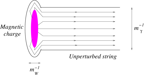
Figure 5: The right-hand half of the broken string (in the ansatz (4.1)). One unit of the magnetic charge is produced in the shaded area. Arrows mark the magnetic field flux.

The kink mass $\tau$ (see Eq. (5.25)) is the mass of the bulge carrying one unit of the magnetic charge. Keeping in mind that $M_{M}\sim V/g$ one may ask why $\tau$ is logarithmically larger than $M_{M}$.

The answer to this question is quite obvious. While the ansatz (4.1) does describe the production of the magnetic charge at the end of the broken string, it is a highly excited monopole-like state rather than the ’t Hooft-Polyakov monopole. Indeed, the longitudinal dimension of the bulge is $\sim m_{W}^{-1}$, a typical size of the monopole core. At the same time its transverse dimension (in the plane perpendicular to the string action) is of order $m_{\gamma}^{-1}$. This is much larger than the monopole core size. The stretching of the core in the perpendicular direction is the reason why this lump is logarithmically heavier than the ’t Hooft-Polyakov monopole. This is an inevitable consequences of the fact that the ansatz (4.1) contains a single profile function $f_{\theta}(r)$ which governs the behavior of both, the photon and the $W$ boson fields.

By introducing two distinct profile functions one can readily eliminate the shortcoming in the ansatz (4.1). We do it in Appendix. However, even before particular improvements are done we want to note that sufficient experience is already accumulated to enable us to develop a proper effective description of the tunneling process.

Indeed, in actuality the end-point domain of the broken string is roughly a hemisphere with the radius $\sim m_{\gamma}^{-1}$. The core which emanates the magnetic flux has dimension of order of $m_{W}^{-1}$ in both transverse and longitudinal directions. In fact, the core is practically unperturbed ’t Hooft-Polyakov monopole. This is due to the fact that at distances of order $m_{W}^{-1}$ the effect of the (magnetic charge) confinement is negligible, it comes into play only at distances $\sim m_{\gamma}^{-1}$. Thus, the mass of the end-point bulge in a “good” ansatz must be $\tau=M_{M}+O(v/g)$. The $O(v/g)$ correction reflects the distortion of the ’t Hooft-Polyakov monopole at distances $\sim m_{\gamma}^{-1}$, and can be neglected compared to $M_{M}$. A potential of the type depicted in Fig. 3 will emerge leading to the tunneling problem described by the bubble action (see Appendix for details),

$$S_{\rm bubble}=2\pi\,\rho M_{M}-\pi\rho^{2}T_{\,\rm ANO}\,.$$ (8.1)

The only distinction with the consideration carried out in Sect. 5.4 is that in the “good” ansatz the ratio of the bubble radius to its thickness

$$\frac{\rho_{*}}{\Delta}\sim\left(\frac{V}{v}\right)$$ (8.2)

(cf. Eq. (5.30)). We loose one power of $V/v$, but the ratio ${\rho_{*}}/{\Delta}$ is still large, and the thin wall approximation justified.

The action (8.1) immediately leads to the string decay rate given in Eq. (1.3). The effective approach based on Eq. (8.1) is exactly the one of Vilenkin [22] and Preskill and Vilenkin [23].

In view of a general nature of this conclusion, let us comment on the hierarchy of parameters we deal with. We want to separate elements of this hierarchy which are absolutely essential for our consideration from those which bear a technical character.

Our consideration is quasiclassical. It is valid only at weak coupling. This requires Eq. (1.1) to be valid. We cannot sacrifice this condition.

Moreover, the two-stage nature of the gauge symmetry breaking, Eq. (1.2), is crucial too. Among other things, it guarantees that the thin wall approximation is justified. It is unclear whether lifting the condition (1.2) one can still develop an analytic description of the tunneling process. We will not try to lift the constraint (1.2).

On the other hand, the relation between $m_{q}$ and $m_{\gamma}$ is clearly of a technical nature. In the two extreme cases, when $m_{q}/m_{\gamma}$ is either very large or very small one can calculate ANO string tension analytically. One can pose a question what happens at arbitrary values of $m_{q}/m_{\gamma}$. Calculation of the ANO string tension in this case certainly requires numerical computations. However, this calculation can be carried out entirely in the macroscopic low-energy U(1) theory, with no reference to the microscopic non-Abelian theory. The procedure is well-developed; the function $F(m_{q}/m_{\gamma})$ which parametrizes the ANO string tension in the general case,

$$T_{\rm ANO}=2\pi v^{2}\,F\left(\frac{m_{q}}{m_{\gamma}}\right)\,,$$ (8.3)

is known in the literature [32].

Irrespective of the value of $m_{q}/m_{\gamma}$, the energy difference in the false and true vacua is ${\cal E}=T_{\rm ANO}$. Moreover, the expression (1.3) for the decay rate is universally valid as long as $\rho_{*}/\Delta\gg 1$, i.e. $V/v\gg 1$. The flat wall tension $\tau$ is calculated in the approximation which neglects the quark field contributions altogether — the barrier is determined only by terms proportional to $V^{2}$. No matter what the particular ansatz is, it must yield $\tau=M_{M}$ modulo possible small correction $\sim v/g$. This condition can be viewed as a test of the “goodness” of the ansatz.

Therefore, if one neglects all terms suppressed by powers of $v/V$ one inevitably arrives at Eq. (8.1), irrespective of the ratio $m_{q}/m_{\gamma}$. The result (1.3) for for the string decay rate $\Gamma_{\rm breaking}$ ensues. It is valid for arbitrary value of the ratio $m_{q}/m_{\gamma}$.

Of particular interest are examples emerging in the supersymmetric setting. For instance, for the BPS string $T_{\rm ANO}=2\pi v^{2}$. Moreover, the BPS bound for the monopole mass $M_{M}$ is

$$M_{M}=\frac{4\sqrt{2}\pi}{g}\,V\,.$$ (8.4)

Then Eq. (1.3) predicts the following decay rate of this string:

$$\Gamma_{\rm BPS}\sim\exp\left\{-\frac{8\pi^{2}}{g^{2}}\,\frac{2\,V^{2}}{v^{2}}\,\right\}\,.$$ (8.5)

Let us recall that the Abelian BPS strings embedded in non-Abelian gauge theories appear, say, in the charge vacua of the Seiberg-Witten theory with matter [14, 29, 30, 17].

9 Comparison with Schwinger’s expression

The decay of the string goes through breaking of the string in pieces through a monopole-antimonopole pair production. From this standpoint, the bubbles of the “true vacuum” of the effective 2D sigma model inside the “false” one are, in fact, domains where the string is broken by monopole-antimonopole pairs. The decay rate is exponentially small for large monopole masses; the exponent is determined by the ratio $M_{M}^{2}/T_{\rm ANO}$.

Given this interpretation it is instructive to compare Eq. (1.3) with the famous Schwinger’s formula [20, 21] for the electron-positron pair production in the constant electric field,

$$\Gamma_{e^{+}e^{-}}\sim\exp\left(-\pi\,\frac{m^{2}}{E}\right)\,,$$ (9.1)

where $m$ is the electron mass, and $E$ is the electric field . Note that with our normalization, see Eq. (2.1), the coupling constant is included in $E$. The probability (9.1) can be obtained as the imaginary part of the one-loop graph presented in Fig. 6.

Figure 6: Propagation of the electric charge in the background electric field. The charged particle loop is denoted by a thick line, the background field by dashed lines.

Dualizing Schwinger’s expression we can try to use it for evaluating the probability of the monopole-antimonopole pair creation in the magnetic field existing in the core of the ANO string. Of course, we have to assume that this field is constant on the scale of the monopole-antimonopole separation (we hasten to add that this is a wrong assumption).

It is not difficult to get from Eq. (9.1) a dualized Schwinger formula for the magnetic monopole pair production in the homogeneous magnetic field. Indeed, with our normalization the duality transformation reads $E\leftrightarrow g^{-2}B$ where $B$ is the magnetic field. Then the dualized Schwinger formula takes the form

$$\Gamma_{M\bar{M}}\sim\exp{\left(-\pi\,\,\frac{M_{M}^{2}}{B\,g^{-2}}\right)}\,.$$ (9.2)

The magnetic field in the ANO string can be readily estimated from its flux,

$$B\sim\frac{2\pi}{\rm area}\sim m_{\gamma}^{2}=\frac{1}{2}\,g^{2}\,v^{2}\,.$$ (9.3)

Combining Eqs. (9.2) and (9.3) one obtains

$$\Gamma_{M\bar{M}}\sim\exp{\left(-\pi\,C\,\frac{M_{M}^{2}}{v^{2}}\right)}\,,$$ (9.4)

where $C$ is a numerical coefficient of order 1.

One might ask whether dualizing Schwinger’s formula is a good idea. Indeed, Schwinger’s formula assumes the smallness of the gauge coupling constant $g^{2}$. The coupling of the magnetic monopoles $\sim g^{-2}$ is then strong. Therefore, the $\gamma$ quanta exchanges, as in Fig. 7, might drastically change the result.

This effect was studied in Ref. [21], where it was found that the extra term in the exponent due to the gamma quanta exchanges is of order $1/g^{2}$. This is easy to understand. Indeed, the corresponding Coulomb energy is of order $1/(\rho_{*}\,g^{2})$ which generates a correction in the bubble action of the order of $1/g^{2}$. It can be safely neglected because $M_{M}^{2}/v^{2}\gg 1/g^{2}$.

Comparing this Schwinger-formula-based expectation with our result (1.3), and keeping in mind that $T_{\rm ANO}=2\pi v^{2}$ modulo a logarithm of $m_{q}/m_{\gamma}$, we see that the powers of the mass scales and of the coupling $g^{2}$ in the two exponents perfectly match each other. However, the logarithmic factors $\left(\ln\,\frac{m_{q}}{m_{\gamma}}\right)^{\kappa}$ are missing in (9.4). These will not (and need not) match, and neither a numerical factor in front of $M_{M}^{2}/v^{2}$. The reason for this is that Schwinger’s formula and our calculation refers to physically different phases of the theory. Schwinger’s formula (9.2) describes monopole-antimonopole production in the external magnetic field in the Coulomb phase while our result (1.3) refers to the breaking of the ANO string by the monopole-antimonopole production in the confinement (for monopoles) phase of the theory.

Figure 7: Propagation of the monopole in the background magnetic field. The monopole loop is denoted by a thick line. $\gamma$ quanta (denoted by a zigzagy line) are strongly coupled to the monopoles, and exchange of the $\gamma$ quanta must be taken into account.

10 Conclusions

In this paper we calculated the decay rate of an Abelian flux tube embedded into a non-Abelian theory. We focussed on two simplest examples where the phenomenon does occur: non-supersymmetric SU(2) gauge theory with the adjoint and fundamental scalars and the same theory with two adjoint scalars. In the first example all ANO strings are metastable. In the second one the string with minimal winding number is stable ($Z_{2}$-string), while strings with multiple winding numbers are metastable.

The pattern of the SU(2) symmetry breaking is two-stage,

$${\rm SU(2)}\stackrel{{\scriptstyle V}}{{\longrightarrow}}{\rm U(1)}\stackrel{{\scriptstyle v}}{{\longrightarrow}}{\rm nothing}\,,\qquad V\gg v\,.$$

As was expected, the decay rate is exponentially small. The suppressing exponent is proportional to the ratio of monopole mass squared to the string tension. The interpretation of this result is that the string gets broken into pieces by the monopole-anti-monopole production. Note that the monopole-anti-monopole pair production in the given context by no means implies that superconductivity is lost.

Although we considered a particular model with metastable strings, we believe that the final answer is rather general and can be qualitatively applied to any metastable Abelian string embedded in a non-Abelian theory. In particular, as we mentioned in Sect. 1, the reduction of string multiplicity from $Z^{N-1}$ down to $Z_{N}$ in the strong coupling vacua of the Seiberg-Witten theory is due to a similar mechanism. In this case we deal with electric strings (which arise due to the monopole /dyon condensation), so that the metastable strings must broken by the $W$ boson pair production (rather than the monopole pair production which takes place in the magnetic flux tubes).

Unwinding ansätze of the type presented in Eq. (4.1) can be used in other similar problems, for instance, for studying the metastability of the appropriately embedded semilocal strings (cf. [23], for a review of the semilocal strings see Ref. [35]).

Finally, it is worth noting that the calculation of the string decay rate presented here can be viewed as a calculation of an open string coupling constant in the effective string theory of ANO string.

Appendix. Improving the primitive unwinding
ansatz

As we explained in Sect. 8 our ansatz (4.1) gives a monopole in a highly exited state at the end of the broken string. Its mass $\tau$ is much larger then the monopole mass due to the logarithmic factor in (5.25). The reason is that we used the same profile function $f_{\theta}$ for both $a=3$ and $a=1,2$ components of the gauge potential in (4.1). We used the model (5.2) for this profile function which ensures that all components of the gauge field are nonvanishing inside the region of size $\sim 1/m_{\gamma}$ in the (1,2)-plane. However, it is clear that the $a=1,2$ components of the gauge field are very heavy (W bosons) and should be spread over a much smaller region, of size $\sim 1/m_{W}$. Now, let us modify the ansatz (4.1) to take this circumstance into account.

First, let us explicitly write down the gauge field given by the ansatz (4.1) in the singular gauge, see Eq. (4.10),

$$A_{i}=-\,\varepsilon_{ij}\,\frac{x_{j}}{r^{2}}\,\left[2\cos^{2}{2\theta}\,\,\frac{\tau_{3}}{2}-\sin{2\theta}\left(\frac{\tau_{1}}{2}\sin{\alpha}+\frac{\tau_{2}}{2}\cos{\alpha}\right)\right]\,f_{\theta}(r)\,.$$ (A.1)

To modify it, we introduce two different profile functions, in front of $\tau_{3}$ and $\tau_{1,2}$ matrices, as follows:

$$A_{i}=-\,\varepsilon_{ij}\,\frac{x_{j}}{r^{2}}\,\left[2\cos^{2}{2\theta}\,\,\frac{\tau_{3}}{2}\,f^{\gamma}_{\theta}(r)-\sin{2\theta}\left(\frac{\tau_{1}}{2}\sin{\alpha}+\frac{\tau_{2}}{2}\cos{\alpha}\right)\,f^{W}_{\theta}(r)\right].$$ (A.2)

We assume that $f^{W}$ is concentrated inside a very small region of size $\sim 1/m_{W}$, whereas $f^{\gamma}$ is spread over a much larger domain of size $\sim 1/m_{\gamma}$. The expressions for the adjoint and the fundamental scalars are still given by Eq. (4.10).

Substituting this into the action (2.1) we end up with

$$T(\theta) = \!\!\!2\pi\int rdr\,\left\{\frac{2}{g^{2}}\,\frac{\cos^{2}{\theta}}{r^{2}}\,\left[\cos^{2}{\theta}(f_{\theta}^{\gamma})^{\prime}\,{}^{2}+\sin^{2}{\theta}(f_{\theta}^{W})^{\prime}\,{}^{2}\right]+q_{\theta}\,^{\prime}\,{}^{2}\right.$$ (A.3)

$$+ \frac{q_{\theta}^{2}}{r^{2}}\,\cos^{2}{\theta}\left(\cos^{2}{\theta}f_{\theta}^{\gamma}+\sin^{2}{\theta}f_{\theta}^{W}\right)$$

$$+ \!\!\!\frac{1}{2}\varphi_{\theta}^{\prime}\,{}^{2}+\frac{1}{2r^{2}}\left[\varphi_{\theta}\left(\cos{2\theta}\,(1-f_{\theta}^{\gamma})-(\cos^{2}{2\theta}f_{\theta}^{\gamma}+\sin^{2}{2\theta}f_{\theta}^{W})\,\right)+Vf^{W}_{\theta}\sin{2\theta}\right]^{2}$$

$$+ \!\!\!\left.\lambda\left(q_{\theta}^{2}-v^{2}\right)^{2}+\tilde{\lambda}\left[\varphi_{\theta}^{2}-2V\varphi_{\theta}\sin{2\theta}\right]^{2}+\frac{\gamma}{4}\varphi_{\theta}^{2}q_{\theta}^{2}\right\}\,.$$

We see that now the term $Vf^{W}_{\theta}\sin{2\theta}$ in the square brackets contains $f^{W}$ rather than $f^{\gamma}$ (cf. Eq. (4.11)). This means that its contribution in the integral will be saturated in a a small region, of size $\sim 1/m_{W}$, and will not lead to large logarithms. Thus, the height of the barrier now is $V^{2}$ instead of $V^{2}\,\ln(m_{a}/m_{\gamma})$. It should be added, however, that in the absence of large logarithms we cannot obtain the barrier profile using analytic calculations. We need computer simulations to minimize the tension (A.3) and find the profile functions. This goes beyond the scope of this paper.

Still, some simple examples of the profile functions we have analyzed show that we can avoid getting large logarithms both in the barrier height and in the kinetic term for the $\theta$ field in the effective 2D sigma model for the unstable string mode. This leads us to the following representation for the domain wall tension $\tau$

$$\tau={\rm const}\;\int\,dz\left\{\frac{1}{g^{2}}\,\left(\partial_{z}\,\theta\right)^{2}+\frac{V^{2}}{4}\,\sin^{2}{2\theta}\right\}\,,$$ (A.4)

instead of the one in Eq. (5.22). Here, the constant in front of this action can be fixed by means of a numerical minimization procedure in (A.3). Note, that the relative coefficient between the kinetic and the potential terms in Eq. (A.4) is fixed by the requirement that the mass of the $\theta$ field should coincide with that of the $W$ boson.

Calculating the domain wall tension in the theory (A.4) we get

$$\tau\,={\rm const}\;\frac{V}{g}\,.$$ (A.5)

In order to prove that actually

$$\tau=M_{M}$$ (A.6)

we need numerical simulations. Still, if we accept on physical grounds that this is the case, then the bubble action in the 2D sigma model given by Eq. (8.1) ensues. This leads us to the final formula (1.3) for the decay rate of the metastable string.

References

- [1] N. Seiberg and E. Witten, Nucl. Phys. B426, 19 (1994) [hep-th/9407087].
- [2] N. Seiberg and E. Witten, Nucl. Phys. B431, 484 (1994), [hep-th/9408099].
- [3] A. Abrikosov, ZhETF 32, 1442 (1957) [Eng. transl. Sov. Phys. JETP, 5, 1174 (1957); reprinted in Solitons and Particles, Eds. C. Rebbi and G. Soliani, (World Scientific, Singapore, 1984), p. 356].
- [4] H. B. Nielsen and P. Olesen, Nucl. Phys. B 61, 45 (1973). [Reprinted in Solitons and Particles, Eds. C. Rebbi and G. Soliani, (World Scientific, Singapore, 1984), p. 365].
- [5] E. B. Bogomolny, Yad. Fiz. 24, 861 (1976) [Engl. transl. Sov. J. Nucl. Phys. 24, 449 (1976); reprinted in Solitons and Particles, Eds. C. Rebbi and G. Soliani, (World Scientific, Singapore, 1984), p. 389].
- [6] H.J. de Vega, Phys. Rev. D18 (1978) 2932.
- [7] H.J. de Vega and F.A. Shaposnik, Phys. Rev. Lett.56 (1986) 2564; Phys. Rev. D34 (1986) 3206.
- [8] J. Heo and T. Vachaspati, Phys. Rev. D58 (1998) 065011 [hep-th/9801455].
- [9] F.A. Shaposnik and P. Suranyi, Phys. Rev. D62 (2000) 125002 [hep-th/0005109].
- [10] M. Kneipp and P. Brockill, Phys. Rev. D64 (2001) 125012 [hep-th/0104171].
- [11] K. Konishi and L. Spanu, “Non-Abelian vortex and confinement”, hep-th/0106175.
- [12] M. Douglas and S. Shenker, Nucl. Phys. B447, 271 (1995) [hep-th/9503163].
- [13] M. Strassler, Prog. Theor. Phys. Suppl. 131, 439 (1998) [hep-th/9803009].
- [14] A. Hanany, M. Strassler and A. Zaffaroni, Nucl. Phys. B513, 87 (1998) [hep-th/9707244].
- [15] A. Yung, Nucl. Phys. B562, 191 (1999) [hep-th/9906243].
- [16] A. Yung, Nucl. Phys. B626, 207 (2002) [hep-th/0103222].
- [17] A. Marshakov and A. Yung, Non-Abelian confinement via Abelian flux tubes in softly broken SUSY QCD, hep-th/0202172.
- [18] G. ’t Hooft, Nucl. Phys. B 79, 276 (1974).
- [19] A. M. Polyakov, Pisma Zh. Eksp. Teor. Fiz. 20, 430 (1974) [Engl. transl. JETP Lett. 20, 194 (1974), reprinted in Solitons and Particles, Eds. C. Rebbi and G. Soliani, (World Scientific, Singapore, 1984), p. 522].
-
[20]
F. Sauter, Z. Phys. 69, 742 (1931);
W. Heisenberg and H. Euler, Z. Phys. 98, 714 (1936);
J. Schwinger, Phys. Rev. 82, 664 (1951). - [21] I. K. Affleck and N. S. Manton, Nucl. Phys. B 194, 38 (1982).
- [22] A. Vilenkin, Nucl. Phys. B 196, 240 (1982).
- [23] J. Preskill and A. Vilenkin, Phys. Rev. D47, 2324 (1993).
- [24] M. B. Voloshin, I. Y. Kobzarev, and L. B. Okun, Yad. Fiz. 20, 1229 (1975) [Sov. J. Nucl. Phys. 20, 644 (1975)].
- [25] S. R. Coleman, Phys. Rev. D 15, 2929 (1977); (E) D 16, 1248 (1977) [Reprinted in The Early Universe, Eds. E.W. Kolb and M.S. Turner, (Addison-Wesley, 1990), p. 483].
-
[26]
Z. Hloušek and D. Spector,
Nucl. Phys. B 370, 143 (1992);
J. Edelstein, C. Nunẽz and F. Schaposnik, Phys. Lett. B 329, 39 (1994) [hep-th/9311055]. - [27] S. C. Davis, A. C. Davis and M. Trodden, Phys. Lett. B 405, 257 (1997) [hep-ph/9702360].
- [28] A. Gorsky and M. A. Shifman, Phys. Rev. D 61, 085001 (2000) [hep-th/9909015].
- [29] W. Fuertes and J. Guilarte, Phys. Lett. B437, 82 (1998) [hep-th/9807218].
- [30] A. I. Vainshtein and A. Yung, Nucl. Phys. B 614, 3 (2001) [hep-th/0012250].
- [31] M. B. Voloshin, False Vacuum Decay, in Vacuum and Vacua: the Physics of Nothing, Proc. International School of Subnuclear Physics, Erice, Italy, July 1995, Ed. A. Zichichi, (World Scientific, Singapore, 1996), p. 88.
- [32] E. B. Bogomolny and A. I. Vainshtein, Yad. Fiz. 23, 1111 (1976) [Sov. J. Nucl. Phys. 23, 588 (1976)].
- [33] C. Bachas and M. Porrati, Phys. Lett. B 296, 77 (1992) [hep-th/9209032].
- [34] A. S. Gorsky, K. A. Saraikin and K. G. Selivanov, Nucl. Phys. B 628, 270 (2002) [hep-th/0110178].
- [35] A. Achucarro and T. Vachaspati, Phys. Rept. 327, 347 (2000) [hep-ph/9904229].