ITFA–2002–11

LPTENS–02–29

A Resolution of the Cosmological
Singularity with Orientifolds

L. Cornalba$\,{}^{\dagger}$, M.S. Costa$\,{}^{\ddagger}$ and C. Kounnas$\,{}^{\ddagger}$

$\,{}^{\dagger}$ Instituut voor Theoretische Fysica, Universiteit van Amsterdam

Valckenierstraat 65, 1018 XE Amsterdam, The Netherlands
lcornalb@science.uva.nl
$\,{}^{\ddagger}$ Laboratoire de Physique Théorique, Ecole Normale Supérieure

24 rue Lhomond, F-75231 Paris Cedex 05, France
miguel@lpt.ens.fr, kounnas@lpt.ens.fr

We propose a new cosmological scenario which resolves the conventional initial singularity problem. The space–time geometry has an unconventional time–like singularity on a lower dimensional hypersurface, with localized energy density. The natural interpretation of this singularity in string theory is that of negative tension branes, for example the orientifolds of type II string theory. Space–time ends at the orientifolds, and it is divided in three regions: a contracting region with a future cosmological horizon; an intermediate region which ends at the orientifols; and an expanding region separated from the intermediate region by a past cosmological horizon. We study the geometry near the singularity of the proposed cosmological scenario in a specific string model. Using D–brane probes we confirm the interpretation of the brane singularity as an orientifold. The boundary conditions on the orientifolds and the past/future transition amplitudes are well defined. Assuming the trivial vacuum in the past, we derive a thermal spectrum in the future.

1 Introduction

Gravity is an attractive force. This is the basic reason for the presence, in the standard cosmological models, of a space–like big–bang singularity in the past. The existence of an initial singularity is, to a large extent, independent of the model, and in fact one can show that, under general assumptions, a singularity in the cosmological past is inevitable [1]. Despite these problems, the standard cosmological models (far) below the Planck scale are extremely successful in explaining the present experimental data.

Attempts to solve the cosmological singularity problem lead to the pre big–bang scenario conjecture [2], motivated by the existence of a minimum distance in string theory. However, either the exact string backgrounds are not realistic [3], or they show time–like singularities whose nature has remained unclear [4, 5, 6]. More recently, the big–bang singularity was investigated in the framework of brane cosmology as collision of branes [7]. However, in these scenarios the cosmological singularity is space–like and does not have a clear interpretation as a brane.

The simplest way to avoid the cosmological singularity is to introduce a bulk positive cosmological constant, which introduces a uniform negative pressure. In the absence of other contributions to the stress–energy tensor one obtains a de Sitter space–time. A de Sitter cosmology is problematic both from the string theory point of view and from a phenomenological view–point. In string theory it has not been possible, up to now, to construct a (meta)–stable string background with a de Sitter geometry. From the cosmological point of view it is difficult to connect a de Sitter phase to the usual matter dominated universes which describe present day evolution of the universe, and at the same time retain a singularity–free space–time.

Although problematic, de Sitter space avoids the cosmological singularity by introducing an effectively repulsive part to the gravitational interaction due to the negative pressure induced by the positive cosmological constant. Another natural way to avoid the big–bang singularity is the introduction of a negative cosmological constant localized on hyperplanes of lower dimension. These lower dimensional branes have negative tension and therefore will fill a repulsive gravitational force induced by standard matter in the bulk. Even though it is problematic in pure gravity to consider objects with negative mass, they appear quite naturally in string theory. Orientifold planes are, for example, hypersurfaces of arbitrary dimension, charged under the Ramond–Ramond fields, with negative tension and no localized dynamical degrees of freedom [8, 9]. From the point of view of gravity, O–planes act as sources of matter and gravity fields by adding a local term in the supergravity action

$$|T|\int_{\Gamma}d^{d}x\,e^{-\phi}\sqrt{-\det G}\ \pm Q\int_{\Gamma}A_{d}\ ,$$

on the $d$–dimensional hypersurface $\Gamma$, where $T$ and $Q$ are the tension and the charge respectively. This acts as a negative cosmological term localized on the surface $\Gamma$, together with the coupling to the other supergravity fields. The geometry which corresponds, in supergravity, to O–planes is similar to the one describing D–branes, but has negative mass and develops a naked time–like singularity.

In this paper we will show that it is possible to resolve the conventional cosmological singularity problem using orientifolds, i.e. by introducing a negative cosmological constant localized on domain walls at the boundary of space–time. The basic idea is to replace the big–bang singularity at $t=0$ by a cosmological horizon and to continue space–time across this horizon. Examples of such space–time causal structure were presented in [4] for a spatially flat cosmology that becomes isotropic at late times and in [6] for isotropic open cosmologies (with hyperbolic spatial sections). Other examples were given in [5]. To understand the existence of this horizon it is convenient to consider the description of $(d+1)$–dimensional flat space–time using the Milne and Rindler ‘polar’ coordinates. Along the ‘cosmological’ Milne wedge the metric depends on the cosmological coordinate $t$, however, as one crosses the horizon the metric dependents on a space–like coordinate $x$, and it is foliated by $d$–dimensional de Sitter slices. The idea proposed in [6], is that one may start integrating the classical equations of motion starting from this horizon regardless of the theory under consideration, imposing the existence of a cosmological horizon. In some cases this space–time causal structure arises as a Kałuża–Klein compactification of flat space–time, which can be described by a string theory orbifold construction, following the earlier work of [10] (see also [11]).

In the specific model we shall consider, which can be embedded in Type II string theory, the geometry in the Rindler patch develops a time–like naked singularity, where the metric has the correct form to be interpreted as an orientifold plane with a de Sitter world–volume (see figure 1). This geometry describes an open universe with contracting and expanding regions, together with an intermediate region bounded by an orientifold plane. The latter region smoothly connects the would be ‘big–crunch’ and ‘big–bang’ of conventional cosmological models. This resolution of the cosmological singularity allows the calculation of transition amplitudes from the contracting to the expanding phases. In particular, we shall calculate the past/future vacuum to vacuum amplitude for a free field propagating in the cosmological background. Assuming a trivial vacuum at the asymptotic past, we obtain a thermal spectrum in the far future. This analysis is similar to that of Hawking in the derivation of black hole radiation [12], but applied to our cosmology.

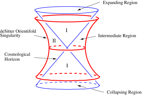
Figure 1: De Sitter orientifold as the boundary of space–time. We shall see that the associated geometry develops a cosmological horizon that allows the smooth transition form a contracting to an expanding cosmological phase.

To describe dynamically the phases of the universe, we can think of a large spherical charged brane as the boundary of the universe, which is contracting due to the brane’s tension. During the collapse, the brane will back–react on the geometry and it will create, in the center of the sphere, a positive energy density. If the brane has positive tension, it will eventually collapse due to its own gravitational and electric forces. On the other hand, if the brane has negative tension, it will interact with its own gravitational and electric fields with opposite sign, and this will invert the contraction to an expanding phase. In this sense, localized negative tension objects can be used to avoid the big–bang singularity.

One may ask at this point why the choice of orientifolds is justified in cosmology. In our point of view this choice has a natural explanation in string theory. Indeed, to create a non–trivial gravitation background with broken supersymmetry one has to start with non–BPS configuration of branes. If not, the vacuum solution will be stable and stationary due to the supersymmetry. One possibility is to construct type II models where the RR charge is canceled only with orientifold planes $O-\overline{O}$ localized in two different points, and without any $D$ or $\overline{D}$ branes. Models of this kind are constructed in the literature [13, 9]. This configuration breaks supersymmetry, and it is incompatible with a flat space–time and constant dilaton. The induced geometry in the presence of $O-\overline{O}$ orientifolds is precisely our cosmological solution. As we shall show in section 3, the $O-\overline{O}$ configuration is stable. There is an attractive electric force which is balanced by an effective repulsive force created by the gravitational back–reaction of the orientifolds. Thus, localized negative tension objects can be used to avoid the conventional big–bang singularity.

Another starting point, is to dress the orientifolds with branes and to consider the configuration $OD-\overline{OD}$. This configuration is consistent classically with a flat space–time and constant dilaton. However, at the quantum level it is unstable due to the lack of supersymmetry. An effective potential is created bringing the branes and anti–branes together which annihilate each other. After this annihilation, we are left with the $O-\overline{O}$ orientifolds, the background fields are no longer flat and give rise to the cosmological scenario described above. We shall confirm the structure of the effective potential among branes and orientifolds by probing the geometry with D–branes. Since orientifolds are a source of the gravitational and RR fields but do not have local degrees of freedom, the acceleration of the universe can be seen effectively from the condensation of the tachyon field associated to the above process. Indeed, tachyon driven time–dependent string backgrounds have been the subject of recent investigation [14] (see [15] for related work).

2 A Simple Cosmological Solution

We start quite generally by considering $\left(d+1\right)$–dimensional gravity coupled to a scalar field $\psi$

$$S=\frac{1}{2\kappa^{2}{\mathcal{E}}^{d-1}}\int d^{d+1}x\sqrt{|g|}\left[R-\frac{\beta}{2}\left(\nabla\psi\right)^{2}-V\left(\psi\right)\right]\ ,$$ (1)

where ${\mathcal{E}}$ is an energy scale. In this equation, $V\left(\psi\right)$ is the potential for the scalar field, $\beta$ is a dimensionless constant and the coordinates are dimensionless in units of $1/{\mathcal{E}}$. Following [6], we are interested in cosmological solutions to the equations of motion of (1) with a contracting and an expanding phase (which we call region $I$), together with an intermediate region (denoted by region $II$). The expanding phase is the standard Robertson–Walker geometry for an open universe

$$\begin{array}[]{rcl}\displaystyle{ds_{d+1}^{\ 2}}&=&\displaystyle{-dt^{2}+a_{I}^{\ 2}\left(t\right)ds^{2}\left(H_{d}\right)}\ ,\phantom{\framebox{\rule[-5.69046pt]{0.0pt}{0.0pt}}}\\ \psi&=&\displaystyle{\psi_{I}\left(t\right)}\ ,\end{array}$$ (2)

where $H_{d}$ is the $d$–dimensional hyperbolic space with unit radius. Therefore, the dynamics of the system is described by the scalar and Friedman equations

$$\begin{array}[]{rcl}\displaystyle{\ddot{\psi}_{I}+d\,\dot{\psi}_{I}\,\frac{\dot{a}_{I}}{a_{I}}}&=&\displaystyle{-\frac{1}{\beta}\,\frac{\partial V}{\partial\psi_{I}}}\ ,\phantom{\framebox{\rule[-14.22636pt]{0.0pt}{0.0pt}}}\\ \displaystyle{\left(\frac{\dot{a}_{I}}{a_{I}}\right)^{2}-\frac{1}{a_{I}^{\ 2}}}&=&\displaystyle{\frac{1}{d\left(d-1\right)}\left[\frac{\beta}{2}\,\dot{\psi}_{I}^{2}+V\left(\psi_{I}\right)\right]}\ ,\end{array}$$ (3)

where dots denote derivatives with respect to the cosmological time $t$. The contracting phase is nothing but the time–reversed solution, where we replace in (2) $t$ by $-t$.

In order to have an intermediate region, we are interested in solutions of (2) where $a_{I}(t)$ and $\psi_{I}(t)$ are, respectively, odd and even functions of $t$ with initial conditions

$$a_{I}\left(t\right)=t+\mathcal{O}\left(t^{3}\right)\ ,\ \ \ \ \ \ \ \ \ \ \ \ \ \ \ \ \ \psi_{I}\left(t\right)=\psi_{0}+\mathcal{O}\left(t^{2}\right)\ ,$$ (4)

for small cosmological time $t$. This implies that the $t=0$ surface does not correspond to a big–bang singularity, but represents a null cosmological horizon, as described in [6]. In this case, the space–time can be extended across the horizon to an intermediate region $II$, where the solution takes the form

$$\begin{array}[]{rcl}\displaystyle{ds_{d+1}^{\ 2}}&=&\displaystyle{a_{II}^{\ 2}\left(x\right)ds^{2}\left(dS_{d}\right)+dx^{2}}\ ,\phantom{\framebox{\rule[-5.69046pt]{0.0pt}{0.0pt}}}\\ \psi&=&\displaystyle{\psi_{II}\left(x\right)}\ ,\end{array}$$ (5)

with $dS_{d}$ the $d$–dimensional de Sitter space. The equations of motion which determine $a_{II}$ and $\psi_{II}$ are again the equations (3), with the potential $V$ replaced by $-V$. To extend the solution from region $I$ to region $II$ it is convenient to write the hyperboloid and de Sitter metrics in conformal coordinates $(i=1,\cdots,d-1)$

$$ds^{2}\left(H_{d}\right)=\frac{dy^{i}dy_{i}+dy_{d}^{\,2}}{y_{d}^{\,2}}\ ,\ \ \ \ \ \ \ \ \ ds^{2}\left(dS_{d}\right)=\frac{-dy_{0}^{\,2}+dy^{i}dy_{i}}{y_{0}^{\,2}}\ .$$

Then, if we consider $a_{I}$ and $\psi_{I}$ as complex functions, the solution can be extended by analytic continuing $t\to ix$, $y_{d}\to iy_{0}$, together with

$$a_{II}\left(x\right)=-ia_{I}\left(ix\right)\ ,\ \ \ \ \ \ \ \ \ \ \ \ \ \ \ \ \ \ \ \ \psi_{II}\left(x\right)=\psi_{I}\left(ix\right)\ .$$

Equivalently, given the boundary conditions (4), regions $I$ and $II$ can be connected along the null cosmological horizon, just as a Milne universe can be glued to a Rindler edge to form flat Minkowski space. Moreover, it is clear that the solution possesses a global $SO\left(1,d\right)$ symmetry, which acts both on $H_{d}$ and on $dS_{d}$.

The existence of an intermediate region demands generically a field theory effective potential whose form is highly restrictive due to the unnatural (fine–tuned) boundary conditions. In the next section we see that string effective supergravity theories provide a Liouville–Toda like potential [16] which naturally respects the boundary conditions at the horizon.

3 Embedding in String Theory

Now let us consider a particular case of the construction of the previous section which can be embedded in Type II string theory. For simplicity we consider backgrounds with a non–trivial RR field. The corresponding ten–dimensional Type II effective action has the form ($l_{s}=2\pi\sqrt{\alpha^{\prime}}$)

$$S=\frac{2\pi}{l_{s}^{\ 8}}\left[\int d^{10}x\sqrt{|g|}e^{-2\phi}\left(R+4\left(\nabla\phi\right)^{2}\right)-\frac{1}{2}\int F\wedge\widetilde{F}\right]\ ,$$

where $F$ is the RR $\left(d+1\right)$–form field strength and $\widetilde{F}=\star F$ is the dual $\widetilde{d}$–form field strength, with $\widetilde{d}=9-d$. A family of solutions, parameterized by an arbitrary constant $g_{s}$, can be constructed by considering the following ansatz

$$\begin{array}[]{c}\displaystyle{{\mathcal{E}}^{2}\,ds^{2}=\Lambda^{-\frac{1}{2}\frac{d+1}{d-1}}\,ds_{d+1}^{\ 2}+\Lambda^{\frac{1}{2}}\,ds^{2}(\mathbb{E}^{\widetilde{d}})}\ ,\phantom{\framebox{\rule[-11.38092pt]{0.0pt}{0.0pt}}}\\ \displaystyle{e^{\phi}=g_{s}\,\Lambda^{\frac{4-d}{4}}\ ,\ \ \ \ \ \ \ \ \ \widetilde{F}=\frac{1}{g_{s}{\mathcal{E}}^{\widetilde{d}-1}}\,\epsilon(\mathbb{E}^{\widetilde{d}})}\ ,\end{array}$$ (6)

where we have defined

$$\Lambda=e^{2\beta\,\psi}\ ,$$

and the line element $ds_{d+1}$ is defined in the previous section. The physical interpretation of the constants $\mathcal{E}$ and $g_{s}$ will become clear below. Following [6], the equations of motion for the scale factor and scalar field are those presented in the previous section with

$$V=\frac{1}{2}\,e^{-\psi}\ ,$$

and

$$\beta=\frac{1}{2}\,\frac{d-1}{3d-2}\ .$$

In [6] it was shown that, in the intermediate region $II$, the geometry develops a time–like curvature singularity. The behavior of the scalar field and scale factor near the singularity was seen to be

$$a_{II}\left(x\right) = a_{s}\left(x_{s}-x\right)^{\gamma}\ ,$$ (7)

$$\psi_{II}\left(x\right) = \log{\left[\eta\left(x_{s}-x\right)\right]^{2}}\ ,$$ (8)

where the constants $\gamma$ and $\eta$ read

$$\gamma=\frac{2\beta}{d-1}\ ,\ \ \ \ \ \ \ \ \ \ \ \ \ \ \ \ \ \ \ \ \eta^{-2}=4\beta\left(1-d\,\gamma\right)\ .$$

The dimensionless constant $a_{s}$ depends on the boundary conditions imposed at the horizon; we shall come back to this issue later. The value of $x_{s}$, where $a\rightarrow 0$ and $\psi\rightarrow-\infty$, can be written as

$$x_{s}=e^{\frac{1}{2}\psi_{0}}c_{s}\ ,$$

where $\psi_{0}$ is the value of the scalar field at the horizon. The constant $c_{s}$ depends only on the dimension $d$ of space and is given numerically by

$\phantom{\framebox{\rule[-2.84544pt]{0.0pt}{0.0pt}}}d^{\phantom{\frac{2}{2}}}$	$2$	$3$	$4$	$5$	$6$	$7$	$8$
$\phantom{\framebox{\rule[-2.84544pt]{0.0pt}{0.0pt}}}c_{s}^{\phantom{\frac{2}{2}}}$	$1.6$	$1.9$	$2.1$	$2.3$	$2.5$	$2.6$	$2.8$

From the behavior of the scalar field at the singularity $(\psi\rightarrow-\infty)$, at the horizon $(\psi=\psi_{0})$ and at the asymptotic future $(\psi\rightarrow+\infty)$, and from the fact that the scalar field is a growing function as one moves from the singularity to the horizon and from there to the asymptotic future, it is natural to use $\Lambda$ as a radial variable instead of $x$. At the singularity we have $\Lambda=0$ and at the lightcone $\Lambda=\Lambda_{0}\equiv e^{2\beta\psi_{0}}$. Then near the singularity, in the limit $\Lambda\ll\Lambda_{0}$, we obtain the following ten–dimensional background fields

$$\begin{array}[]{c}\displaystyle{\mathcal{E}^{2}ds^{2}=\Lambda^{-\frac{1}{2}}\,\mu\,ds^{2}(dS_{d})+\Lambda^{\frac{1}{2}}\left[d\Lambda^{2}+ds^{2}(\mathbb{E}^{\widetilde{d}})\right]}\ ,\phantom{\framebox{\rule[-14.22636pt]{0.0pt}{0.0pt}}}\\ \displaystyle{e^{\phi}=g_{s}\Lambda^{\frac{4-d}{4}}\ ,\ \ \ \ \ \ \ \ \ \ \ \ \ F=-\frac{1}{g_{s}\mathcal{E}^{d}}\,d\Lambda^{-1}\wedge\left[\sqrt{\mu^{d}}\,\epsilon(dS_{d})\right]}\ ,\end{array}$$

where $\mu$ is a constant determined from the constant $a_{s}$ in the expansion (8). If we substitute the de Sitter space $dS_{d}$ by the Minkowski space $\mathbb{M}^{d}$ we obtain naively the solution for D$p$–branes $(p=d-1)$ localized at $\Lambda=0$ and uniformly smeared along $\mathbb{E}^{\widetilde{d}}$. The usual harmonic function $H$ is simply $H=\Lambda$ because there a unique transverse direction. However, the tension associated with the harmonic function proportional to $-\bigtriangleup H$ is negative. Therefore the singularity is correctly interpreted as non–dynamical orientifold $(d-1)$–planes smeared along the $\mathbb{E}^{\widetilde{d}}$. When $\Lambda\rightarrow 0$ the radius of the de Sitter slice $\sqrt{\mu}\,\Lambda^{-1/4}$ diverges, the orientifold looks flat and one approaches the usual supersymmetric solution. This solution is interpreted as the geometry of a de Sitter O$p$–plane ($p=d-1$) with radius $R_{dS}\sim 1/\mathcal{E}$ and delocalized along $\mathbb{E}^{\widetilde{d}}$. Below we shall compute the number of orientifold planes in terms of the parameters of the solution.

To understand the behavior of the geometry away from the orientifold planes it is useful to keep using the function $\Lambda$ as the radial coordinate. Then the solution (6) becomes

$$\begin{array}[]{c}\displaystyle{\mathcal{E}^{2}ds^{2}=\frac{G}{\Lambda^{\frac{1}{2}}}\,\mu\,ds^{2}\left(dS_{d}\right)+\frac{\Lambda^{\frac{1}{2}}}{H}d\Lambda^{2}+\Lambda^{\frac{1}{2}}ds^{2}(\mathbb{E}^{\widetilde{d}})}\ ,\phantom{\framebox{\rule[-17.07182pt]{0.0pt}{0.0pt}}}\\ \displaystyle{e^{\phi}=g_{s}\Lambda^{\frac{4-d}{4}}\ ,\ \ \ \ \ \ \ \ \ \ \ \ \ \ \ F=\frac{1}{g_{s}\mathcal{E}^{d}}\,\frac{1}{\Lambda^{2}}\sqrt{\frac{G^{d}}{H}}\,d\Lambda\wedge\left[\sqrt{\mu^{d}}\,\epsilon(dS_{d})\right]}\ ,\end{array}$$ (9)

where $G(\Lambda)$ and $H(\Lambda)$ are dimensionless functions defined by

$$\mu\,G=\Lambda^{-\frac{1}{d-1}}\,a_{II}^{\ 2}(\Lambda)\ ,\ \ \ \ \ \ \ \ \ \ \ \ \ \ \ \ \ \ \ H=\Lambda^{\frac{d}{d-1}}\left(\frac{d\Lambda}{dx}\right)^{2}\ .$$

Notice that, to match the near singularity behavior, the function G satisfies $G(0)=1$. Naively the solution is parameterized by $g_{s}$, $\mathcal{E}$ and the position of the horizon $\Lambda_{0}$. However, we can set

$$\Lambda_{0}=1\ ,$$

using the rescaling of the coordinates $\Lambda\to c\Lambda$ and $\mathbb{E}^{\widetilde{d}}\to c\,\mathbb{E}^{\widetilde{d}}$, which leaves the form of the solution invariant if we also redefine $g_{s}\to c^{(d-4)/4}\,g_{s}\,$, $\mathcal{E}\to c^{5/4}\,\mathcal{E}$ and $G(\Lambda)\to c^{3}G(\Lambda)$, $H(\Lambda)\to H(\Lambda)$.

With this rescaling the parameters $g_{s}$ and $\mathcal{E}$ are the string coupling $e^{\phi}$ and the electric field $g_{s}\sqrt{-F^{2}}$ at the core of the solution, i.e. at the cosmological horizon. In terms of these parameters we can compute the number of orientifold planes. To this end we compactify the transverse space on a torus $\mathbb{T}^{\widetilde{d}}$ with proper volume at the horizon

$$V=\mathcal{E}^{-\widetilde{d}}\int_{\mathbb{T}^{\widetilde{d}}}\epsilon(\mathbb{E}^{\widetilde{d}})\ .$$

Then the number of O–planes is given by

$$N=\frac{2^{\,6-d}}{l_{s}^{\ 8-d}}\int_{\mathbb{T}^{\widetilde{d}}}\widetilde{F}=2^{\,6-d}\,\,\frac{l_{s}\mathcal{E}}{g_{s}}\,\frac{V}{l_{s}^{\ \widetilde{d}}}\ .$$

Now let us analyze the behavior of the solution near $\Lambda=1$ and near $\Lambda=0$. It is easy to show, from the boundary conditions (4) on the cosmological horizon, that

$$G\left(1\right)=H\left(1\right)=0\ .$$ (10)

To analyze analytically the behavior close to the singularity, we need to rewrite the scalar and Friedman equations in terms of $G$ and $H$ as functions of $\Lambda$. It is tedious but not difficult to show that equations (3) are equivalent to

$$\begin{array}[]{rcl}\displaystyle{\left(\frac{G^{\prime}}{G}\right)^{2}+\frac{2}{(d-1)\Lambda}\,\frac{G^{\prime}}{G}}&=&\displaystyle{\frac{4\Lambda}{\mu GH}+\frac{2}{d(d-1)\Lambda^{2}}\left(1-\frac{1}{H}\right)}\ ,\phantom{\framebox{\rule[-19.91684pt]{0.0pt}{0.0pt}}}\\ \displaystyle{\frac{H^{\prime}}{H}+d\,\frac{G^{\prime}}{G}}&=&\displaystyle{\frac{2}{\Lambda}\,\left(1-\frac{1}{H}\right)}\ ,\end{array}$$ (11)

where ^′ denotes derivative with respect to $\Lambda$. Then we see that, to keep the behavior of the solution near the orientifold at $\Lambda=0$, we must have

$$H\left(0\right)=1\ .$$

On the other hand, when solving the equations starting from the singularity, we are free to choose the initial condition

$$G^{\prime}\left(0\right)=-\sigma\ ,$$

for arbitrary $\sigma$. Then, equations (11) can be solved in power series in $\Lambda$ to give

$$\begin{array}[]{l}\displaystyle{G\,=\,1-\frac{\sigma}{\mu}\,\Lambda-\frac{\sigma^{2}}{\mu^{2}}\,\frac{d-1}{2}\,\Lambda^{2}+\cdots}\ ,\phantom{\framebox{\rule[-14.22636pt]{0.0pt}{0.0pt}}}\\ \displaystyle{H\,=\,1-\frac{\sigma}{\mu}\,d\,\Lambda+\frac{\sigma^{2}}{\mu^{2}}\,\frac{d\left(d-1\right)}{2}\Lambda^{2}+\cdots}\ .\end{array}$$ (12)

Notice that for $d=1$ the solution can be found exactly [6] because the geometry arises as a quotient of flat space and the functions $G$ and $H$ are linear in $\Lambda$.

We have seen that, starting from the orientifold singularity at $\Lambda=0$ we have two degrees of freedom $\mu$ and $\sigma$ in the solution of (11). On the other hand, starting from the light–cone we do not have any freedom. Therefore the solutions that develop a cosmological horizon (10) correspond to a special value of $\mu$ and $\sigma$. For the cosmological solutions we are analyzing, these constants depend only on the spatial dimension $d$ and are given numerically by

$\phantom{\framebox{\rule[-5.69046pt]{0.0pt}{0.0pt}}}d^{\phantom{\frac{2}{2}}}$	$1$	$2$	$3$	$4$	$5$	$6$	$7$	$8$
$\phantom{\framebox{\rule[-5.69046pt]{0.0pt}{0.0pt}}}\mu^{\phantom{\frac{2}{2}}}$	$1$	$4.5$	$5.2$	$5.9$	$6.7$	$7.4$	$8.2$	$8.9$
$\phantom{\framebox{\rule[-5.69046pt]{0.0pt}{0.0pt}}}\sigma^{\phantom{\frac{2}{2}}}$	$1$	$3.1$	$2.9$	$2.9$	$2.9$	$2.9$	$2.9$	$2.9$

For large cosmological times in region $I$ the geometry is that of a curvature dominated universe.

3.1 Probing the Geometry with Branes

Now that we have seen the string theoretic origin of the cosmological singularity and how the geometry behaves as we move away from the orientifolds, we would like to study the motion of D–branes in this geometry. We are going to consider a spherical brane on the de Sitter slices $dS_{d}$, positioned in region $II$ at some fixed value of $\Lambda<\Lambda_{0}$, and we are going to compute the static potential $\mathcal{V}\left(\Lambda\right)$ seen by the brane. Notice that by static potential we mean the potential as seen by an observer on the brane, i.e. an observer placed at constant $\Lambda$.

It is well known that, in the case of flat branes, there is a brane/anti–orientifold repulsion, whereas there is no force between parallel branes and orientifolds (of opposite charge), due to the BPS nature of the configuration. In the present case, we will see that the presence of a de Sitter world volume of both the source and the probe brane induces a repulsive force also on the probe branes with charge opposite to that of the orientifold singularity. The force, when the probe is placed close to the source, is repulsive and tends to move the probe brane away from the singularity. Bellow we shall argue that the force inducing the brane probe to collapse is partially gravitational in character and arises from the energy density of the fields generated by the de Sitter orientifolds. This same energy density will act as an anti–gravitational force on the orientifolds preventing them from collapse. This mechanism provides a smooth transition from a big–crunch to a big–bang phase, which is regular in string theory and should allow the computation of transition amplitudes from the contracting to the expanding region. Section four gives the simplest example of such computation.

The static potential for a spherical D$p$–brane ($p=d-1$) in the cosmological background can be deduced starting from the metric (9). An easy calculation shows that the Born–Infeld and the Wess–Zumino pieces give a total action

$$\mathcal{V}_{\pm}\left(\Lambda\right)=\frac{1}{\Lambda}\sqrt{G^{d}}\mp\int\frac{d\Lambda}{\Lambda^{2}}\sqrt{\frac{G^{d}}{H}}\ .$$

The potential $\mathcal{V}_{+}$ ($\mathcal{V}_{-}$) is the potential seen by a probe with charge equal (opposite) to those of the orientifolds forming the singularity. Using the solution (12) we easily see that

$$\mathcal{V}_{+}\left(\Lambda\right)=\frac{2}{\Lambda}+\cdots\ ,$$

and therefore $\mathcal{V}_{+}$ represents, as expected, a strongly repulsive potential. As we discussed above, the potential $\mathcal{V}_{-}$ is more interesting physically, and vanishes for the case of parallel flat branes and orientifolds. Again using (12) one can show that

$$\mathcal{V}_{-}\left(\Lambda\right)=-\frac{d}{2}\,\frac{\sigma}{\mu}-\frac{d\left(3d-2\right)}{8}\,\frac{\sigma^{2}}{\mu^{2}}\,\Lambda+\cdots\ .$$

Note that, as long as $\sigma\neq 0$ (as it is the case for the cosmological solutions), the potential decreases as a function of $\Lambda$ for any value of $d\geq 1$, and therefore there is a repulsive force which moves the probe away from the singularity at $\Lambda=0$. One could think that this repulsive force is only due to the tension of the spherical brane probe. On the other hand, the analysis of the $d=1$ case, where the tension is absent, shows that this intuition is not entirely correct.

Let us consider a $O-\overline{O}$ pair in flat space at some large distance and a $D$ particle near the $O$ plane. The only force on the $D$ particle is the gravitational and electric repulsive force due to the $\overline{O}$ plane, since a $OD$ pair is a BPS configuration. Now let us turn on gravity and consider the back–reaction on the geometry due to the presence of the orientifolds. For this case we can define a coordinate $y$ by $\Lambda=1-y^{4}$, such that $y\in]-1,0[$ corresponds to the part of region $II$ with the $O$ plane, and $y\in]0,1[$ corresponds to the part with the $\overline{O}$ plane. We recall that $y=0$ is the horizon where this coordinate system becomes singular. Then, recalling that $G=H=1-\Lambda$, the potential in the whole of region $II$ is given by (see figure 2)

$$\mathcal{V}_{D}(y)=\frac{y^{2}}{1-y^{2}\,{\mathrm{s}ign}(y)}\ .$$

The fields generated by the orientifolds induce an energy density between them, which interacts gravitationally with the $D$–particle. Indeed, this computation shows that the latter gravitational attraction wins over the $D-\overline{O}$ repulsion. We conclude that the force that brings the $D$ particle away from the $O$–plane is due to the back–reaction on the geometry, which is creating an extra energy density that interacts gravitationally with the probe.

Figure 2: The potential $\mathcal{V}_{D}$ seen by a $D$–brane probe in the geometry created by the $O-\overline{O}$ system, for $d=1$. The potential repels the $D$–brane from both the $O$ and the $\overline{O}$–plane. The vertical dashed line represents the location of the cosmological horizon.

This energy density induced by the orientifolds is also responsible for the repulsion between the O–planes, explaining the structure of the geometry against the naive expectation that the $O-\overline{O}$ system is unstable under collapse and annihilation. To confirm this interpretation let us show that the electric field at the center of the exact solution is larger than the electric field generated by the $O-\overline{O}$ system if we had neglected back–reaction. This shows that the extra energy density is concentrated at the center of the geometry. At the center, which is at a proper distance $L$ from the orientifolds given by

$$\mathcal{E}L\,=\int_{0}^{1}\frac{\Lambda^{\frac{1}{4}}}{\sqrt{1-\Lambda}}d\Lambda\,=\frac{2\sqrt{2}}{21\sqrt{\pi}}\,\Gamma\left[\,1/4\,\right]^{2}\,\simeq\,1.75\ ,$$

the electric field of the exact solution couples to gravity with strength $\mathcal{E}$. On the other hand, in flat space–time and assuming linear superposition, the electric field of a $O-\overline{O}$ system at distance $2L$ is given in the intermediate point by

$$\frac{8}{5\,L}<\mathcal{E}\ ,$$

thus confirming our claim.

In the general case, the $O-\overline{O}$ pair is really a spherical orientifold and the energy density around the center of the geometry gravitationally attracts the brane probes. Moreover, the same energy density prevents the orientifold sphere from collapsing, and is actually the cause of the transition from the contracting to the expanding phases.

4 Thermal Radiation from the Past Cosmological Vacuum

We wish to analyze the propagation of matter in the cosmological backgrounds studied in the previous sections. For simplicity, we shall consider the case $d=1$ which arises [6] as an orbifold of Minkowski space under a combined boost and translation.

Let us consider a scalar field $\Xi$ of mass $m$ in three–dimensional Minkowski space ${\mathbb{M}}^{3}$ with coordinates $X^{\pm}=T\pm X$ and $Y$, which satisfies the usual Klein–Gordon equation

$$\left(-\nabla^{2}+m^{2}\right)\Xi=\left(4\partial_{+}\partial_{-}-\partial^{\ 2}_{Y}+m^{2}\right)\Xi=0\ .$$

We want to consider solutions of this equation which are invariant under the identification $\Gamma$ defined by $X^{\pm}\sim e^{\pm 2\pi\Delta}X^{\pm}$ and $Y\sim Y+2\pi R$. We conveniently define the energy scale $E$ to be $E=\Delta/R$. These identifications are trivially satisfied with the separation of variables

$$\Xi\left(X^{+},X^{-},Y\right)=\chi\left(X^{+},X^{-}\right)e^{-ipEY}\ ,$$

where $\chi$ satisfies

$$\chi\left(e^{\sigma}X^{+},e^{-\sigma}X^{-}\right)=e^{iJ\sigma}\chi\left(X^{+},X^{-}\right)\ ,$$ (13)

for any $\sigma$ and where

$$J=p+\frac{n}{\Delta}\ .$$

The integer $n$ is the Kałuża–Klein charge, and from now on we shall consider the uncharged $n=0$ case. In this case the Klein–Gordon equation becomes

$$\left(4\partial_{+}\partial_{-}+(\omega E)^{2}\right)\chi=0\ ,$$ (14)

where

$$\omega^{2}=\left(\frac{m}{E}\right)^{2}+p^{2}\ .$$

It is clear that $\chi$ satisfies the Klein–Gordon equation in two–dimensional flat space for a particle of effective mass $\omega E$ and lorentzian spin $J$. Such equation is naturally solved by introducing lorentzian polar coordinates in the Milne and Rindler edges of the two–dimensional flat space–time, which correspond respectively to regions $I$ and $II$ of the cosmological solution. The polar coordinates read

$$\begin{array}[]{ll}{\mathrm{R}egion\ }I:&EX^{\pm}=t\,e^{\pm z}\phantom{\framebox{\rule[-2.84544pt]{0.0pt}{0.0pt}}}\\ {\mathrm{R}egion\ }II:&EX^{\pm}=\pm x\,e^{\pm s}\end{array}$$ (15)

and the boost (13) acts as spatial translation along $z$ and time translation along $s$ in the two regions, respectively. Therefore the linearly independent solutions to (14) are (see [17] and references therein)

$$\begin{array}[]{ll}{\mathrm{R}egion\ }I:&e^{ipz}\,\mathcal{H}_{p}(\omega t)\ ,\ \ \ \ \ \ \ \ \ \,e^{ipz}\,\mathcal{H}_{p}(-\omega t)\phantom{\framebox{\rule[-5.69046pt]{0.0pt}{0.0pt}}}\\ {\mathrm{R}egion\ }II:&e^{ips}\,\mathcal{H}_{p}(i\omega|x|)\ ,\ \ \ \ \ \ e^{ips}\,\mathcal{H}_{p}(-i\omega|x|)\end{array}$$

where $\mathcal{H}_{p}$ is a properly normalized Hankel function

$$\mathcal{H}_{p}(v)=\sqrt{\frac{\pi}{2}}e^{-\frac{\pi}{2}|p|}\,H^{(1)}_{i|p|}(v)\ ,$$

with the property that

$$\overline{\mathcal{H}_{p}(v)}=\pm\mathcal{H}_{p}(-\overline{v})\ ,\ \ \ \ \ \ \ \ \ \pm{\mathrm{I}m}(v)<0\ ,$$

and with asymptotic behavior

$$\mathcal{H}_{p}(v)\simeq\frac{1}{\sqrt{v}}\,e^{iv-i\frac{\pi}{4}}\ ,\ \ \ \ \ \ \ \ \ |v|\gg 1\ .$$

To solve for the scalar field $\chi$ it remains to fix the boundary condition at the singularity at $-E^{2}X^{+}X^{-}=x^{2}=1$. At the end of this section we will embed this three–dimensional model $\mathbb{M}^{3}/\Gamma$ in M–theory, and the compactification on $\mathbb{M}^{3}/\Gamma\times\mathbb{E}^{8}$ will yield the $d=1$ cosmology of the previous sections. With this in mind we can fix the behavior of the field $\chi$ at the singularity. From the orientifold construction there are two possible boundary conditions. Either the field $\chi$ vanishes at the singularity, or its normal derivative $\partial_{x}\chi$ does. This depends on which Type II particle the field $\chi$ describes. For simplicity of exposition we will explicitly consider only the Dirichlet boundary condition. The other possibility is similar.

It is convenient to expand the quantum field $\chi$ starting from region $II$ and to write

$$\begin{array}[]{rcl}\chi&=&e^{ips+i\frac{\pi}{4}}\left[i\,A\,\mathcal{H}_{p}(i\omega|x|)+B\,\mathcal{H}_{p}(-i\omega|x|)\right]a(p)\phantom{\framebox{\rule[-8.5359pt]{0.0pt}{0.0pt}}}\\ &&+\,e^{-ips-i\frac{\pi}{4}}\left[i\,A\,\mathcal{H}_{p}(i\omega|x|)+B\,\mathcal{H}_{p}(-i\omega|x|)\right]a^{\dagger}(p)\ ,\end{array}$$

where $a(p)$ and $a^{\dagger}(p)$ are annihilation and creation operators. The constants $A$ and $B$ are chosen real and positive and are normalized so that

$$A^{2}-B^{2}=1\ .$$

Moreover, the Dirichlet boundary condition gives

$$\frac{B}{A}=\left|\frac{\mathcal{H}_{p}(i\omega)}{\mathcal{H}_{p}(-i\omega)}\right|\ .$$

We need to continue the quantum field above to the contracting and expanding regions $I$. This involves an analytic continuation of $i|x|$ to $\pm t$. In particular, we will choose the continuation $i|x|\to t+i\epsilon$ for the function multiplying the annihilation operator $a(p)$ and the opposite continuation $-i|x|\to t-i\epsilon$ for the function associated with $a^{\dagger}(p)$ [12]. Note that we must introduce an infinitesimal parameter $\epsilon>0$ to correctly define the function near the branch cut of $\mathcal{H}_{p}(v)$ on the negative real axis. With such prescription the field in region $I$ has the form

$$\begin{array}[]{rcl}\chi&=&e^{ipz+i\frac{\pi}{4}}\left[i\,A\,\mathcal{H}_{p}(\omega t+i\epsilon)+B\,\mathcal{H}_{p}(-\omega t-i\epsilon)\right]a(p)\phantom{\framebox{\rule[-8.5359pt]{0.0pt}{0.0pt}}}\\ &&+\,e^{-ipz-i\frac{\pi}{4}}\left[i\,A\,\mathcal{H}_{p}(-\omega t+i\epsilon)+B\,\mathcal{H}_{p}(\omega t-i\epsilon)\right]a^{\dagger}(p)\ .\end{array}$$

The above choice of creation and annihilation operators defines the quantum field starting from the singularity, and defines what we call the intermediate vacuum, i.e. the natural vacuum for a static observer in region $II$.

We will now show that the constants $A$ and $B$ are the Bogolubov coefficients which relate the intermediate vacuum to the natural vacua of the contracting and expanding phases in region $I$. Firstly consider the contracting region in the far past $t\ll-1$, where the field $\chi$ becomes

$$\chi\simeq\frac{1}{\sqrt{|\omega t|}}\left[e^{i(\omega t+pz)}\,a_{\,\mathrm{i}n}(p)+e^{-i(\omega t+pz)}\,a_{\,\mathrm{i}n}^{\dagger}(p)\right]\ ,$$ (16)

with

$$\begin{array}[]{c}\displaystyle{a_{\,\mathrm{i}n}(p)=A\,a(p)+B\,a^{\dagger}(-p)}\ ,\phantom{\framebox{\rule[-5.69046pt]{0.0pt}{0.0pt}}}\\ \displaystyle{a^{\dagger}_{\,\mathrm{i}n}(p)=B\,a(-p)+A\,a^{\dagger}(p)}\ .\end{array}$$

Similarly, in the expanding region for $t\gg 1$ the field is given by

$$\chi\simeq\frac{1}{\sqrt{\omega t}}\left[i\,e^{i(\omega t+pz)}\,a_{\,\mathrm{o}ut}(p)-i\,e^{-i(\omega t+pz)}\,a_{\,\mathrm{o}ut}^{\dagger}(p)\right]\ ,$$ (17)

where the creation and annihilation operators read

$$\begin{array}[]{c}\displaystyle{a_{\,\mathrm{o}ut}(p)=A\,a(p)-B\,a^{\dagger}(-p)}\ ,\phantom{\framebox{\rule[-5.69046pt]{0.0pt}{0.0pt}}}\\ \displaystyle{a^{\dagger}_{\,\mathrm{o}ut}(p)=-B\,a(-p)+A\,a^{\dagger}(p)}\ .\end{array}$$

Therefore we conclude that

$$\begin{array}[]{c}\displaystyle{a_{\,\mathrm{o}ut}(p)=\alpha\,a_{\,\mathrm{i}n}(p)-\beta\,a^{\dagger}_{\,\mathrm{i}n}(-p)}\ ,\phantom{\framebox{\rule[-5.69046pt]{0.0pt}{0.0pt}}}\\ \displaystyle{a^{\dagger}_{\,\mathrm{o}ut}(p)=-\beta\,a_{\,\mathrm{i}n}(-p)+\alpha\,a^{\dagger}_{\,\mathrm{i}n}(p)}\ ,\end{array}$$

where

$$\alpha=A^{2}+B^{2}\ ,\ \ \ \ \ \ \ \ \ \ \ \beta=2AB\ .$$

The natural choice for the cosmological vacuum is the past vacuum $\left|0\right>$ defined by $a_{\,\mathrm{i}n}(p)\left|0\right>=0$. Hence, the observer in the expanding universe will detect an average number $N(p)$ of particles of momentum $p$ given by

$$N(p)=|\beta|^{2}\ .$$

Notice that these particles arise from the reflection on the orientifold singularity. Indeed the non–trivial coefficient $\beta$ in the Bogolubov transformation relates states with equal and opposite momentum. Moreover, we can define an effective dimensionless temperature

$$\frac{1}{{\mathcal{T}}(\omega)}=\frac{1}{\omega}\,\ln\left|\frac{\alpha}{\beta}\right|^{2}=\frac{2}{\omega}\,\ln\frac{1}{2}\left(\left|\frac{\mathcal{H}_{p}(i\omega)}{\mathcal{H}_{p}(-i\omega)}\right|+\left|\frac{\mathcal{H}_{p}(-i\omega)}{\mathcal{H}_{p}(i\omega)}\right|\right)\ .$$

For $\omega\gg 1,\,m/E$ the effective temperature approaches a constant

$${\mathcal{T}}\simeq\frac{1}{2\pi}\ .$$

In this limit ${\mathcal{T}}$ has the standard form $\kappa/2\pi$, where $\kappa=1$ is either the surface gravity of the horizon with respect to the killing vector field $\partial_{s}$ or the acceleration of the orientifold mirror in the dimensionless coordinates $EX^{\pm}$.

Figure 3: The effective temperature $2\pi{\mathcal{T}}$ as a function of $\omega$.

As we already mentioned, to embed this construction in the $d=1$ string theory cosmological model of the previous sections we need only to add eight spectator flat directions and consider the M–theory compactification on $({\mathbb{M}}^{3}/\Gamma)\times{\mathbb{E}}^{8}$. We concentrate on the massless M–theory fields and therefore we set $m=0$. Then the Einstein metric and the other fields are

$$\begin{array}[]{c}\displaystyle{E^{2}ds^{2}=\Lambda^{\frac{1}{8}}\left[-dt^{2}+ds^{2}(\mathbb{E}^{8})\right]+\Lambda^{-\frac{7}{8}}t^{2}dz^{2}}\ ,\phantom{\framebox{\rule[-8.5359pt]{0.0pt}{0.0pt}}}\\ \displaystyle{e^{\phi}=g_{s}\,\Lambda^{\frac{3}{4}}=g_{s}\left(1+t^{2}\right)^{\frac{3}{4}}\ ,\ \ \ \ \ \ \ \ \ \ F=-\frac{2}{g_{s}E}\,d\Lambda^{-1}\wedge\,dz}\ .\end{array}$$

The eleven–dimensional Klein–Gordon equation for the massless scalar field $\Xi$ reduces to

$$\nabla^{2}\chi=0\ ,$$

which is equation (14) in the lorentzian polar coordinates (15) for $m=0$.

The comoving cosmological observer will measure a red–shifted local energy given by

$$\Omega=\frac{\omega}{\sqrt{-g_{tt}}}=\Lambda^{-\frac{1}{16}}\,E\omega\ ,$$

and a physical temperature

$$T=\Lambda^{-\frac{1}{16}}E\,{\mathcal{T}}(\omega)\ .$$

For fixed $\Omega$ at large cosmological times, the associated dimensionless frequency $\omega$ is blue shifted and we obtain an exact thermal spectrum with temperature

$$T=\frac{E}{2\pi\,a(\tau)}\ ,$$

where $a(\tau)$ is the scale factor and $\tau$ the proper cosmological time.

We can extend this result to the $(d+1)$–dimensional cosmological solutions of the previous sections. To do this one just needs to compute the surface gravity of the cosmological horizon with respect to the appropriate Killing vector field. The natural Killing vector fields to use are the generators of the $SO(1,d)$ isometries. One has to be careful with the normalization of the vector field which is space–like in region $I$. With this in mind, one arrives at the general result

$$T=\frac{{\mathcal{E}}}{2\pi\,a(\tau)}\ .$$ (18)

This is expected for radiation in a $(d+1)$–dimensional cosmology, since from Boltzmann law $\rho\sim T^{d+1}$ we obtain $\rho\sim 1/a^{d+1}(\tau)$, which follows from the radiation equation of state $\rho=d\,p$.

5 Conclusion

In this work we show that the presence of a localized negative cosmological constant on a time–like lower dimensional hypersurface avoids the conventional space–like singularity of the big–crunch/big–bang scenarios. This localized energy density arises naturally in string theory as branes with negative tension like orientifolds. The resulting non–trivial cosmological background has a horizon, which is created naturally in orientifold models with broken supersymmetry. Space–time is divided in three regions. Firstly, there is a collapsing region with a future cosmological horizon. As we pass this horizon, we enter a ‘static’ region with the localized orientifolds. This region has a future horizon. Crossing this horizon we enter the expanding phase. The key idea is that the existence of the horizon flips the would be space–like singularity to a time–like singularity leading to a brane resolution of the singularity.

To study the generic properties of the proposed cosmological scenario we consider a specific model in string theory. The interpretation of the singularity as an orientifold was justified by analyzing the geometry near the singularity and by probing it with D–branes. The analysis of this effective potential showed that there is an energy density at the core of the geometry, which prevents the orientifolds to collapse due to the gravitational repulsion. Also, the resolution of the singularity provides well defined boundary conditions, which are necessary to determine past/future transition amplitudes. In particular, we considered the vacuum to vacuum amplitude. Assuming the trivial vacuum in the past, we derived a thermal spectrum for radiation in the far future with temperature given by equation (18).

References

- [1] S. W. Hawking and G. F. R. Ellis, The large scale structure of space–time, Cambridge Monographs on Mathematical Physics, Cambridge University Press (1973).
- [2] G. Veneziano, String cosmology: The pre-big bang scenario, hep-th/0002094.
- [3] E. Kiritsis and C. Kounnas, String gravity and cosmology: Some new ideas, gr-qc/9509017.
- [4] C. Kounnas and D. Lust, Cosmological string backgrounds from gauged WZW models, Phys. Lett. B 289 (1992) 56, hep-th/9205046.
- [5] C. Grojean, F. Quevedo, G. Tasinato and I. Zavala C., Branes on charged dilatonic backgrounds: Self-tuning, Lorentz violations and cosmology, JHEP 0108, 005 (2001), hep-th/0106120.
- [6] L. Cornalba and M.S. Costa, A New Cosmological Scenario in String Theory, hep-th/0203031.
-
[7]
A. Kehagias and E. Kiritsis,
Mirage cosmology,
JHEP 9911 (1999) 022, hep-th/9910174.
J. Khoury, B. A. Ovrut, P. J. Steinhardt and N. Turok, The ekpyrotic universe: Colliding branes and the origin of the hot big bang, Phys. Rev. D 64 (2001) 123522, hep-th/0103239.
S. H. Alexander, Inflation from D - anti-D brane annihilation, Phys. Rev. D 65 (2002) 023507, hep-th/0105032.
G. R. Dvali, Q. Shafi and S. Solganik, D-brane inflation, hep-th/0105203.
C. P. Burgess, M. Majumdar, D. Nolte, F. Quevedo, G. Rajesh and R. J. Zhang, The inflationary brane-antibrane universe, JHEP 0107 (2001) 047,
hep-th/0105204.
C. Herdeiro, S. Hirano and R. Kallosh, String theory and hybrid inflation / acceleration JHEP 0112 (2001) 027, hep-th/0110271.
C. P. Burgess, P. Martineau, F. Quevedo, G. Rajesh and R. J. Zhang, Brane-antibrane inflation in orbifold and orientifold models, JHEP 0203 (2002) 052, hep-th/0111025.
J. Garcia-Bellido, R. Rabadan and F. Zamora, Inflationary scenarios from branes at angles, JHEP 0201 (2002) 036, hep-th/0112147.
K. Dasgupta, C. Herdeiro, S. Hirano and R. Kallosh, D3/D7 inflationary model and M-theory, hep-th/0203019. - [8] J. Polchinski, TASI lectures on D-branes, hep-th/9611050.
- [9] C. Angelantonj and A. Sagnotti, Open strings, hep-th/0204089.
-
[10]
J. Khoury, B. A. Ovrut, N. Seiberg, P. J. Steinhardt and N. Turok,
From big crunch to big bang, hep-th/0108187.
N. Seiberg, From big crunch to big bang - is it possible?, hep-th/0201039. -
[11]
V. Balasubramanian, S. F. Hassan, E. Keski-Vakkuri and A. Naqvi,
A space-time orbifold: A toy model for a cosmological singularity,
hep-th/0202187.
N. A. Nekrasov, Milne universe, tachyons, and quantum group, hep-th/0203112.
J. Simon, The geometry of null rotation identifications, hep-th/0203201.
H. Liu, G. Moore and N. Seiberg, Strings in a Time-Dependent Orbifold, hep-th/0204168.
S. Elitzur, A. Giveon, D. Kutasov and E. Rabinovici, From Big Bang to Big Crunch and Beyond, hep-th/0204189. - [12] S. W. Hawking, Particle Creation by Black Holes, Commun. Math. Phys. 43 (1975) 199.
-
[13]
I. Antoniadis, E. Dudas and A. Sagnotti,
Supersymmetry breaking, open strings and M-theory,
Nucl. Phys. B 544 (1999) 469, hep-th/9807011.
S. Kachru, J. Kumar and E. Silverstein, Orientifolds, RG flows, and closed string tachyons, Class. Quant. Grav. 17 (2000) 1139, hep-th/9907038.
C. Angelantonj, E. Dudas and J. Mourad, Orientifolds of String Theory Melvin backgrounds, (CERN-TH/2002-091) to appear. -
[14]
M. Gutperle and A. Strominger,
Spacelike branes,
JHEP 0204 (2002) 018, hep-th/0202210.
A. Sen, Rolling tachyon, hep-th/0203211; Tachyon matter, hep-th/0203265; Field theory of tachyon matter, hep-th/0204143.
G. W. Gibbons, Cosmological evolution of the rolling tachyon, hep-th/0204008.
M. Fairbairn and M. H. Tytgat, Inflation from a tachyon fluid?, hep-th/0204070.
A. Feinstein, Power-law inflation from the rolling tachyon, hep-th/0204140. -
[15]
C. M. Chen, D. V. Gal’tsov and M. Gutperle,
S-brane solutions in supergravity theories,
hep-th/0204071.
M. Kruczenski, R. C. Myers and A. W. Peet, Supergravity S-branes, hep-th/0204144.
J. Kumar, A brief comment on Instanton-like Singularities and Cosmological Horizons, hep-th/0204119.
O. Aharony, M. Fabinger, G. Horowitz and E. Silverstein, Clean Time-Dependent String Backgrounds from Bubble Baths, hep-th/0204158. - [16] I. Antoniadis and C. Kounnas, The Dilaton Classical Solution And The Supersymmetry Breaking Evolution In An Expanding Universe, Nucl. Phys. B 284 (1987) 729.
- [17] A. J. Tolley and N. Turok, Quantum fields in a big crunch / big bang spacetime, hep-th/0204091.