Dilaton Gravity in Two Dimensions

Abstract

The study of general two dimensional models of gravity allows to tackle basic questions of quantum gravity, bypassing important technical complications which make the treatment in higher dimensions difficult. As the physically important examples of spherically symmetric Black Holes, together with string inspired models, belong to this class, valuable knowledge can also be gained for these systems in the quantum case. In the last decade new insights regarding the exact quantization of the geometric part of such theories have been obtained. They allow a systematic quantum field theoretical treatment, also in interactions with matter, without explicit introduction of a specific classical background geometry. The present review tries to assemble these results in a coherent manner, putting them at the same time into the perspective of the quite large literature on this subject.

, ,

Contents

toc

1 Introduction

The fundamental difficulties encountered in the numerous attempts to merge quantum theory with General Relativity by now are well-known even far outside the narrow circle of specialists in these fields. Despite many valiant efforts and new approaches like loop quantum gravity [371] or string theory a final solution is not in sight. However, even many special questions search an answer.

Of course, at energies which will be accessible experimentally in the foreseeable future, due to the smallness of Newton’s constant, respectively the large value of the Planck mass, an effective quantum theory of gravity can be constructed [129] in a standard way which in its infrared asymptotical regime as an effective quantum theory may well describe our low energy world. Its extremely small corrections to classical General Relativity (GR) are in full agreement with experimental limits [436]. However, the fact that Newton’s constant carries a dimension, inevitably makes perturbative quantum gravity inconsistent at energies of the order of the Planck mass.

In a more technical language, starting from a fixed classical background, already a long time ago perturbation theory has shown that although pure gravity is one-loop renormalizable [404] this renormalizability breaks down at two loops [188], but already at one-loop when matter interactions are taken into account. Supergravity was only able to push the onset of non-renormalizability to higher loop order (cf. e.g. [224, 38, 119]). It is often argued that a full treatment of the metric, including non-perturbative effects from the backreaction of matter, may solve the problem but to this day this remains a conjecture. A basic conceptual problem of a theory like gravity is the double role of geometric variables which are not only fields but also determine the (dynamical) background upon which the physical variables live. This is e.g. of special importance for the uncertainty relation at energies above the Planck scale leading to Wheeler’s notion of “space-time-foam” [434].

Another question which has baffled theorists is the problem of time. In ordinary quantum mechanics the time variable is set apart from the “observables”, whereas in the straightforward quantum formulation of gravity (the so-called Wheeler-deWitt equation [435, 121]) a variable like time must be introduced more or less by hand through “time-slicing”, a multi-fingered time etc. [232]. Already at the classical level of GR “time” and “space” change their roles when passing through a horizon which leads again to considerable complications in a Hamiltonian approach [10, 272].

Measuring the “observables” of usual quantum mechanics one realizes that the genuine measurement process is related always to a determination of the matrix element of some scattering operator with asymptotically defined ingoing and outgoing states. For a gauge theory like gravity, existing proofs of gauge-independence for the $S$-matrix [279] may be applicable for asymptotically flat quantum gravity systems. But the problem of other experimentally accessible (gauge independent!) genuine observables is open, when the dynamics of the geometry comes into play in a nontrivial manner, affecting e.g. the notion what is meant by asymptotics.

The quantum properties of black holes (BH) still pose many questions. Because of the emission of Hawking radiation [211, 412], a semi-classical effect, a BH should successively lose energy. If there is no remnant of its previous existence at the end of its lifetime, the information of pure states swallowed by it will have only turned into the mixed state of Hawking radiation, violating basic notions of quantum mechanics. Thus, of special interest (and outside the range of methods based upon the fixed background of a large BH) are the last stages of BH evaporation.

Other open problems – related to BH physics and more generally to quantum gravity – have been the virtual BH appearing as an intermediate stage in scattering processes, the (non-)existence of a well-defined $S$-matrix and $CPT$ (non-)invariance. When the metric of the BH is quantized its fluctuations may include “negative” volumes. Should those fluctuations be allowed or excluded? The intuitive notion of “space-time foam” seems to suggest quantum gravity induced topology fluctuations. Is it possible to extract such processes from a model without ad hoc assumptions? From experience of quantum field theory in Minkowski space one may hope that a classical singularity like the one in the Schwarzschild BH may be eliminated by quantum effects – possibly at the price of a necessary renormalization procedure. Of course, the latter may just reflect the fact that interactions with further fields (e.g. other modes in string theory) are not taken into account properly. Can this hope be fulfilled?

In attempts to find answers to these questions it seems very reasonable to always try to proceed as far as possible with the known laws of quantum mechanics applied to GR. This is extremely difficult in $D=4$. Therefore, for many years a rich literature developed on lower dimensional models of gravity. The $2D$ Einstein-Hilbert action is just the Gauss-Bonnet term. Therefore, intrinsically $2D$ models are locally trivial and a further structure is introduced. This is provided by the dilaton field which naturally arises in all sorts of compactifications from higher dimensions. Such models, the most prominent being the one of Jackiw and Teitelboim (JT), were thoroughly investigated during the 1980-s [22, 123, 405, 122, 124, 238, 250, 251, 312, 388]. An excellent summary (containing also a more comprehensive list of references on literature before 1988) is contained in the textbook of Brown [59]. Among those models spherically reduced gravity (SRG), the truncation of $D=4$ gravity to its s-wave part, possesses perhaps the most direct physical motivation. One can either treat this system directly in $D=4$ and impose spherical symmetry in the equations of motion (e.o.m.-s) [276] or impose spherical symmetry already in the action [36, 412, 33, 409, 205, 324, 407, 244, 276, 295, 195], thus obtaining a dilaton theory. Classically, both approaches are equivalent.

The rekindled interest in generalized dilaton theories in $D=2$ (henceforth GDTs) started in the early 1990-s, triggered by the string inspired [310, 137, 443, 127, 316, 233, 117, 254] dilaton black hole model, studied in the influential paper of Callan, Giddings, Harvey and Strominger (CGHS) [71]. At approximately the same time it was realized that $2D$ dilaton gravity can be treated as a non-linear gauge-theory [426, 230].

As already suggested by earlier work, all GDTs considered so far could be extracted from the dilaton action [373, 349]

$$L^{(\textrm{dil})}=\int d^{2}x\,\sqrt{-g}\;\left[X\frac{R}{2}-\frac{U(X)}{2}\;(\nabla X)^{2}+V(X)\;\right]+L^{(m)}\,,$$ (1.1)

where $R$ is the Ricci-scalar, $X$ the dilaton, $U(X)$ and $V(X)$ arbitrary functions thereof, $g$ is the determinant of the metric $g_{\mu\nu}$, and $L^{(m)}$ contains eventual matter fields.

When $U(X)=0$ the e.o.m. for the dilaton from (1.1) is algebraic. For invertible $V^{\prime}(X)$ the dilaton field can be eliminated altogether, and the Lagrangian density is given by an arbitrary function of the Ricci-scalar. A recent review on the classical solution of such models is ref. [381]. In comparison with that, the literature on such models generalized to depend also on torsion $T^{a}$ is relatively scarce. It mainly consists of elaborations based upon a theory proposed by Katanaev and Volovich (KV) which is quadratic in curvature and torsion [250, 251], also known as “Poincaré gauge gravity” [322].

A common feature of these classical treatments of models with and without torsion is the almost exclusive use of the gauge-fixing for the $D=2$ metric familiar from string theory, namely the conformal gauge. Then the e.o.m.-s become complicated partial differential equations. The determination of the solutions, which turns out to be always possible in the matterless case ($L^{(m)}=0$ in (1.1)), for nontrivial dilaton field dependence usually requires considerable mathematical effort. The same had been true for the first papers on theories with torsion [250, 251]. However, in that context it was realized soon that gauge-fixing is not necessary, because the invariant quantities $R$ and $T^{a}T_{a}$ themselves may be taken as variables in the KV-model [390, 389, 391, 392]. This approach has been extended to general theories with torsion.

As a matter of fact, in GR many other gauge-fixings for the metric have been well-known for a long time: the Eddington-Finkelstein (EF) gauge, the Painlevé-Gullstrand gauge, the Lemaître gauge etc. . As compared to the “diagonal” gauges like the conformal and the Schwarzschild type gauge, they possess the advantage that coordinate singularities can be avoided, i.e. the singularities in those metrics are essentially related to the “physical” ones in the curvature. It was shown for the first time in [291] that the use of a temporal gauge for the Cartan variables (cf. eq. (3.3) below) in the (matterless) KV-model made the solution extremely simple. This gauge corresponds to the EF gauge for the metric. Soon afterwards it was realized that the solution could be obtained even without previous gauge-fixing, either by guessing the Darboux coordinates [377] or by direct solution of the e.o.m.-s [290] (cf. sect. 3.1). Then the temporal gauge of [291] merely represents the most natural gauge fixing within this gauge-independent setting. The basis of these results had been a first order formulation of $D=2$ covariant theories by means of a covariant Hamiltonian action in terms of the Cartan variables and further auxiliary fields $X^{a}$ which (beside the dilaton field $X$) take the role of canonical momenta (cf. eq. (2.17) below). They cover a very general class of theories comprising not only the KV-model, but also more general theories with torsion. The most attractive feature of theories of type (2.17) is that an important subclass of them is in a one-to-one correspondence with the GDT-s (1.1). This dynamical equivalence, including the essential feature that also the global properties are exactly identical, seems to have been noticed first in [248] and used extensively in studies of the corresponding quantum theory [281, 285, 284].

Generalizing the formulation (2.17) to the much more comprehensive class of “Poisson-Sigma models” [379, 396] on the one hand helped to explain the deeper reasons of the advantages from the use of the first oder version, on the other hand led to very interesting applications in other fields [3], including especially also string theory [382, 387]. Recently this approach was shown to represent a very direct route to $2D$ dilaton supergravity [140] without auxiliary fields.

Apart from the dilaton BH [71] where an exact (classical) solution is possible also when matter is included, general solutions for generic $D=2$ gravity theories with matter cannot be obtained. This has been possible only in restricted cases, namely when fermionic matter is chiral [278] or when the interaction with (anti)selfdual scalar matter is considered [356].

Semi-classical treatments of GDT-s take the one loop correction from matter into account when the classical e.o.m.-s are solved. They have been used mainly in the CGHS-model and its generalizations [41, 117, 374, 44, 115, 147, 256, 446, 445, 209, 210, 423]. In our present report we concentrate only upon Hawking radiation as a quantum effect of matter on a fixed (classical) geometrical background, because just during the last years interesting insight has been obtained there, although by no means all problems have been settled.

Finally we turn to the full quantization of GDTs. It was believed by several authors (cf. e.g. [373, 349, 242, 139, 138]) that even in the absence of interactions with matter nontrivial quantum corrections exist and can be computed by a perturbative path integral on some fixed background. Again the evaluation in the temporal gauge [291], at first for the KV-model showed that the use of other gauges just obscures a very simple mechanism. Actually all divergent counter-terms can be absorbed into one compact expression. After subtracting that in the absence of matter the solution of the classical theory represents an exact “quantum” result. Later this perturbative argument has been reformulated as an exact path integral, first again for the KV-model [204] and then for general theories of gravity in $D=2$ [281, 285, 284, 196, 157, 199].

In our present review we concentrate on the path integral approach, with Dirac quantization only referred to for sake of comparison. In any case, the common starting point is the Hamiltonian analysis which in a theory formulated in terms of Cartan variables in $D=2$ possesses substantial technical advantages. The constraints, even in the presence of matter interactions, form an algebra with momentum-dependent structure constants. Despite that nonlinearity the simplest version of the Batalin-Vilkovisky procedure [27] suffices, namely the one also applicable to ordinary nonabelian gauge theories in Minkowski space. With a temporal gauge fixing for the Cartan variables also used in the quantized theory, the geometric part of the action yields the exact path integral. Possible background geometries appear naturally as homogeneous solutions of differential equations which coincide with the classical ones, reflecting “local quantum triviality” of $2D$ gravity theories in the absence of matter, a property which had been observed as well before in the Dirac quantization of the KV-model [377].

These features are very difficult to locate in the GDT-formulation (1.1), but become evident in the equivalent first order version with a “Hamiltonian” action.

Of course, non-renormalizability persists in the perturbation expansion when the matter fields are integrated out. But as an effective theory in cases like spherically reduced gravity, specific processes can be calculated, relying on the (gauge-independent) concept of $S$-matrix elements. With this method, scattering of s-waves in spherically reduced gravity has provided a very direct way to create a “virtual” BH as an intermediate state without further assumptions [157].

The structure of our present report is determined essentially by the approach described in the last paragraphs. One reason is the fact that a very comprehensive overview of very general classical and quantum theories in $D=2$ is made possible in this manner. Also a presentation seems to be overdue in which results, scattered now among many different original papers can be integrated into a coherent picture. Parallel developments and differences to other approaches will be included in the appropriate places.

1.1 Structure of this review

This review is organized as follows:

• Section 1 in its remaining part contains a short primer on differential geometry (with special emphasis on $D=2$). En passant most of our notations are fixed in that subsection.

• Section 2 motivates the study of GDTs and introduces its action in the three most frequently used forms (dilaton action, first order action, and Poisson-Sigma action) and describes the relations between them.

• Section 3 gives all classical solutions of GDTs in the absence of matter. The global structure of such theories is discussed using Schwarzschild space-time as a simple example. As a further illustration we consider a family of dilaton models describing a single black hole in Minkowski, Rindler or de Sitter space-time.

• Section 4 extends the discussion to additional gauge-fields, supergravity and (bosonic or fermionic) matter fields.

• Section 5 considers the role of energy in GDTs. In particular, the ADM mass, quasilocal energy, an absolute conservation law and its corresponding Nöther symmetry are discussed.

• Section 6 leaves the classical realm providing a concise treatment of (semi-classical) Hawking radiation for minimally and non-minimally coupled matter.

• Section 7 is devoted to non-perturbative path integral quantization of the geometric sector of GDTs with (scalar) matter, giving rise to a non-local and non-polynomial effective action depending solely on the matter fields and external sources. The matter sector is treated perturbatively.

• Section 8 shows some consequences of the previously developed perturbation theory: the virtual black hole phenomenon, the appearance of non-local vertices, and $S$-matrix elements for $s$-wave gravitational scattering.

• Section 9 describes the status of Dirac quantization for a typical example of that approach.

• Section 10 concludes with a brief summary and an outlook regarding open questions.

• Appendix A recalls the spherical reduction procedure in the Cartan formalism.

• Appendix B collects some basic properties of the heat kernel expansion needed in Section 6.

Several topics are closely related to the subject of this review, but are not included:

1. Various calculations and explanations of the BH entropy [169, 355] became a large and rather independent field of research which shows, however, overlaps [165, 171] with the general treatment of the dilaton theories presented in this review. We do not cover approaches which imply further physical assumptions which transgress the orthodox application of quantum theory to gravity [34, 35, 43, 24, 31].

2. The ideas of the holographic principle [403, 400] and of the AdS/CFT correspondence [309, 200, 444] are now being actively applied to BH physics (see, e.g. [375] and references therein).

3. There exist different approaches to integrability of gravity models in two dimensions [338, 269, 268, 339]. In particular, a rather sophisticated technique has been applied to solve the effective $2D$ models emerging after toroidal reduction (instead of the spherical reduction considered in this review) of the four-dimensional Einstein equations [39, 417]. Recently again interesting developments should be noted in Liouville gravity [151, 406]. Some relations between $2D$ dilaton gravity and the theory of solitons were discussed in [70, 336].

Each of these topics deserves a separate review, and in some cases such reviews exist. Therefore, we have restricted ourselves in those fields to just a few (somewhat randomly selected) references which hopefully will permit further orientation.

1.2 Differential geometry

1.2.1 Short primer for general dimensions

In the comprehensive approach advocated for $D=2$ gravity the use of Cartan variables (zweibeine, spin-connection) plays a pivotal role. As an introduction and in order to fix our notations we shall review briefly this formalism. For details we refer to the mathematical literature (cf. e.g. [334]).

On a manifold with $D$ dimensions in each point one introduces vielbeine $e^{\mu}_{a}(x)$, where Greek indices refer to the (holonomic) coordinates $x^{\mu}=(x^{0},x^{1},\dots,x^{D-1})$ and Latin indices denote the ones related to a (local) Lorentz frame with metric $\eta=\mbox{diag}~{}(1,-1,\dots,-1)$. The dual vector space is spanned by the inverse vielbeine $e^{a}_{\mu}(x)$:

$$e^{\mu a}e_{\mu}^{b}=\eta^{ab}$$ (1.2)

$SO(1,D-1)$ matrices $L^{a}{}_{b}(x)$ of the (local) Lorentz transformations obey

$${L^{a}}_{c}\,{L_{b}}^{c}\;=\;\delta^{a}_{b}\;.$$ (1.3)

A Lorentz vector $V^{a}=e^{a}_{\mu}V^{\mu}$ transforms under local Lorentz transformations as

$${V^{\prime}}^{a}(x)={L^{a}}_{b}(x)V^{b}(x)$$ (1.4)

This implies a covariant derivative

$${(D_{\mu})^{a}}_{b}\;=\;\delta^{a}_{b}\,\partial_{\mu}+\omega_{\mu}{}^{a}{}_{b}\;,$$ (1.5)

if the spin-connection $\omega_{\mu}{}^{a}{}_{b}$ is introduced as the appropriate gauge field with transformation

$$\omega^{\prime}_{\mu}{\,}^{a}{}_{b}\;=-L{}_{b}{}^{d}\;(\partial_{\mu}L^{a}{}_{d})+L^{a}{}_{c}\,\omega_{\mu}{}^{c}{}_{d}\,L_{b}{}^{d}\;.$$ (1.6)

The infinitesimal version of (1.6) follows from $L^{a}{}_{b}=\delta^{a}{}_{b}+l^{a}{}_{b}+\mathcal{O}(l^{2})$ where $l^{a}{}_{b}=-l_{b}{}^{a}$ .

Formally also diffeomorphisms

$${\bar{x}}^{\mu}(x)=x^{\mu}-\xi^{\mu}(x)+\mathcal{O}(\xi^{2})$$ (1.7)

can be interpreted, at least locally, as gauge transformations, when the Lie variation is employed which implies a transformation referring to the same point. In

$$\frac{\partial{\bar{x}}^{\mu}}{\partial x^{\nu}}=\delta_{\nu}^{\mu}-\xi^{\mu}_{,\,\nu}\;,\hskip 14.22636pt\frac{\partial x^{\nu}}{\partial{\bar{x}}^{\mu}}=\delta^{\nu}_{\mu}+\xi^{\nu}_{,\,\mu}$$ (1.8)

partial derivatives with respect to $x^{\nu}$ have been abbreviated by the index after a comma.

For instance, for the Lie variation of a tensor of first order ${\bar{V}}_{\mu}(\bar{x})=\frac{\partial x^{\nu}}{\partial{\bar{x}}^{\mu}}\,V_{\nu}(x)$ one obtains

$$\delta_{\xi}V_{\mu}(x)={\bar{V}}_{\mu}(x)-V_{\mu}(x)={\xi^{\nu}},{}_{\mu}\,V_{\nu}+\xi^{\nu}V_{\mu},{}_{\nu}\;.$$ (1.9)

For the dual to the tangential space, e.g. $V^{\mu}\partial_{\mu}=V^{\mu}(\partial_{\mu}{\bar{x}}^{\nu})\bar{\partial}_{\nu}={\bar{V}}^{\mu}{\bar{\partial}}_{\mu}$ one derives the analogous transformation

$$\delta_{\xi}V^{\mu}={\bar{V}}^{\mu}(x)-V^{\mu}(x)=-{\xi^{\mu}},{}_{\nu}V^{\nu}+\xi^{\nu}{V^{\mu}},{}_{\nu}\;.$$ (1.10)

The metric $g_{\mu\nu}$ in the line element is a quadratic expression of the vielbeine

$$(ds)^{2}=g_{\mu\nu}\,dx^{\mu}dx^{\nu}=e_{\mu}^{a}e_{\nu}^{b}\,\eta_{ab}\,dx^{\mu}dx^{\nu}\,,$$ (1.11)

and, therefore, a less elementary variable. Also the reparametrization invariant volume element

$$\sqrt{(-)^{D-1}g}\;d^{D}\,x=\sqrt{(-)^{D-1}\det g_{\mu\nu}}\,d^{D}\,x=\\ =\sqrt{(-)^{D-1}(\det e_{\mu}^{a})^{2}\,\det\eta}\,d^{D}\,x=|\det e_{\mu}^{a}|\,d^{D}{}x=|e|\,d^{D}{}x$$ (1.12)

is of polynomial form if expressed in vielbein components.

The advantage of the form calculus [334] is that diffeomorphism invariance is automatically implied, when the Cartan variables are converted into one forms

$$e_{\mu}^{a}\;\rightarrow\;e^{a}=e^{a}_{\mu}dx^{\mu},\hskip 14.22636pt\omega_{\mu}{}^{a}{}_{b}\;\rightarrow\;\omega^{a}{}_{b}=\omega_{\mu}{}^{a}{}_{b}\,dx^{\mu}$$ (1.13)

which are special cases of p-forms

$$\Omega_{p}=\frac{1}{p!}\,\Omega_{\mu_{1}\,\dots\;\mu_{p}}\,dx^{\mu_{1}}\wedge dx^{\mu_{2}}\wedge\dots\wedge dx^{\mu_{p}}\;.$$ (1.14)

Due to the antisymmetry of the wedge product $dx^{\mu}\wedge dx^{\nu}=dx^{\mu}\otimes dx^{\nu}-dx^{\nu}\otimes dx^{\mu}=-dx^{\nu}\wedge dx^{\mu}$ all totally antisymmetric tensors $\Omega_{\mu_{1}\dots\mu_{p}}$ are described in this way. Clearly $\Omega_{p}=0$ for $p>D$. The action of the $(p+q)$-form $\Omega_{q}\wedge\Omega_{q}$ on $p+q$ vectors is defined by

$$\Omega_{p}\wedge\Xi_{q}(V_{1},\dots,V_{p+q})=\frac{1}{p!q!}\sum_{\pi}\delta_{\pi}\Omega(V_{\pi(1)},\dots,V_{\pi(p)})\Xi(V_{\pi(p+1)},\dots,V_{\pi(p+q)}),$$ (1.15)

where the sum is taken over all permutations $\pi$ of $1,\dots,p+q$ and $\delta_{\pi}$ is $+1$ for an even number of transpositions and $-1$ for an odd number of transpositions. It is convenient at this point to introduce the condensed notation for (anti)symmetrization:

$$\alpha_{[\mu_{1}\dots\mu_{p}]}:=\frac{1}{p!}\sum_{\pi}\delta_{\pi}\alpha_{a_{\pi(1)}\dots a_{\pi(p)}},\hskip 14.22636pt\sigma_{(\mu_{1}\dots\mu_{p})}:=\frac{1}{p!}\sum_{\pi}\sigma_{a_{\pi(1)}\dots a_{\pi(p)}},$$ (1.16)

where the sum is taken over all permutations $\pi$ of $1,\dots,p$ and $\delta_{\pi}$ is defined as before. In the volume form

$$\Omega_{p=D}=\frac{1}{D!}a_{[\mu_{1}\dots\mu_{D}]}\;\tilde{\epsilon}^{\mu_{1}\,\dots\;\mu_{D}}\,d^{D}x=\frac{1}{D!}a_{[\mu_{1}\,\dots\;\mu_{D}]}\,|e|\epsilon^{\mu_{1}\,\dots\;\mu_{D}}d^{D}x$$ (1.17)

the product of differentials must be proportional to the totally antisymmetric Levi-Civitá symbol $\tilde{\epsilon}^{01\dots(D-1)}=-1$ or, alternatively, to the tensor $\epsilon=|e|^{-1}\tilde{\epsilon}$ (cf. (1.12)). The integral of the volume form $\int_{\mathcal{M}_{D}}\Omega_{D}$ on the manifold $\mathcal{M}_{D}$ contains the scalar $a=a_{[\mu_{1}\,\dots\;\mu_{D}]}\,\epsilon^{\mu_{1}\,\dots\;\mu_{D}}$ which is the starting point to construct diffeomorphism invariant Lagrangians.

By means of the metric (1.11) a mixed $\epsilon$-tensor

$${\epsilon_{\mu_{1}\,\dots\;\mu_{p}}}{}^{\mu_{p+1}\,\dots\;\mu_{p+q}}\;=\;g_{\mu_{1}\nu_{1}}\,g_{\mu_{2}\nu_{2}}\,\dots\,g_{\mu_{p}\nu_{p}}\,\epsilon^{\nu_{1}\,\dots\,\nu_{p}\mu_{p+1}\dots\mu_{p+q}}$$ (1.18)

can be defined which allows the introduction of the Hodge dual of $\Omega_{p}$ as a $D-p$ form

$${}^{\ast}\,\Omega_{p}\;=\;{\Omega^{\prime}}_{D-p}=\frac{1}{p!(D-p)!}\epsilon_{\mu_{1}\,\dots\,\mu_{D-p}}{}^{\nu_{1}\,\dots\,\nu_{p}}\;\Omega_{\nu_{1}\,\dots\,\nu_{p}}\;dx^{\mu_{1}}\,\wedge\,\dots\,\wedge dx^{\mu_{D-p}}\;.$$ (1.19)

In $D=\rm even$ and for Lorentzian signature we obtain for a p-form

$$\ast\ast\Omega_{p}=(-1)^{p+1}\Omega_{p}.$$ (1.20)

The exterior differential one form $d=dx^{\mu}\partial_{\mu}$ with $d^{2}=0$ increases the form degree by one:

$$d\Omega_{p}=\frac{1}{p!}\partial_{\mu}\Omega_{\mu_{1}\dots\mu_{p}}dx^{\mu}\wedge dx^{\mu_{1}}\wedge\dots\wedge dx^{\mu_{p}}$$ (1.21)

Onto a product of forms $d$ acts as

$$d\left(\Omega_{p}\wedge\Omega_{q}\right)=d\Omega_{p}\wedge\Omega_{q}+(-1)^{p}\Omega_{p}\wedge d\Omega_{q}\;.$$ (1.22)

We shall need little else from the form calculus [334] except the Poincaré Lemma which says that for a closed form, obeying $d\Omega_{p}=0$, in a certain (“star-shaped”) neighborhood of a point $x^{\mu}$ on a manifold $\mathcal{M}$, $\Omega_{p}$ is exact, i.e. can be written as $\Omega_{p}=d{\Omega^{\prime}}_{p-1}$.

In order to simplify our notation we shall drop the $\wedge$ symbol whenever the meaning is clear from the context.

The Cartan variables expressed as one forms (1.13) in view of their Lorentz-tensor properties are examples of algebra valued forms. This is also the case for the covariant derivative (1.5), now written as

$$D^{a}{}_{b}\;=\;\delta^{a}_{b}d+\omega^{a}{}_{b}\;,$$ (1.23)

when it acts on a Lorentz vector.

From (1.13) and (1.23) the two natural quantities to be defined on a manifold are the torsion two-form

$$T^{a}\;=\;D^{a}{}_{b}\,e^{b}$$ (1.24)

(“First Cartan’s structure equation”) and the curvature two-form

$$R^{a}{}_{b}=D^{a}{}_{c}\,\omega^{c}{}_{b}\;$$ (1.25)

(“Second Cartan’s structure equation”). From (1.23) immediately follows

$$(D^{2})^{a}{}_{b}=D^{a}{}_{c}D^{c}{}_{b}=R^{a}{}_{b}\,,$$ (1.26)

Bianchi’s first identity. Using (1.26) $D^{3}$ can be written in two equivalent ways,

$$D^{a}{}_{b}\,R^{b}{}_{c}-R^{a}{}_{b}\,D^{b}{}_{c}=0,$$ (1.27)

corresponding to Bianchi’s second identity

$$(dR^{ab})+\omega^{a}{}_{c}R^{cb}+\omega^{b}{}_{c}R^{ac}\;=:\;(DR)^{ab}=0\;.$$ (1.28)

The l.h.s. defines the action of the covariant derivative (1.23) on $R^{ab}$, a Lorentz tensor with two indices. The brackets indicate that those derivatives only act upon the quantity $R$ and not further to the right. The structure equations together with the Bianchi identities show that the covariant action for any gravity action in $D$ dimensions depending on $e^{a},\omega^{a}{}_{b}$ can be constructed as a volume form depending solely on $R^{ab},\,T^{a}$ and $e^{a}$. The most prominent example is Einstein gravity in $D=4$ [136, 135] which in the Palatini formulation reads [352]

$$L_{HEP}\;\propto\;\int\limits_{\mathcal{M}_{4}}\;R^{ab}e^{c}e^{d}\;\epsilon_{abcd}\;,$$ (1.29)

having used the definition $\epsilon_{abcd}=\epsilon_{\mu\nu\sigma\tau}e_{a}^{\mu}e_{b}^{\nu}e_{c}^{\sigma}e_{d}^{\tau}$. The condition of vanishing torsion $T^{a}=0$ for this special case already follows from varying $\omega^{a}{}_{b}$ independently in (1.29).

In the usual textbook formulations of Einstein gravity, in terms of the metric, the affine connection $\Gamma_{\mu\nu}{}^{\rho}$ appears as the only variable in the covariant derivative, e.g. for a contravariant vector $X^{\nu}$

$$X^{\nu}_{;\,\mu}:=\nabla_{\mu}\,X^{\nu}=(\nabla_{\mu})^{\nu}{}_{\rho}\,X^{\rho}=(\partial_{\mu}\delta^{\nu}_{\rho}+\Gamma_{\mu\rho}{}^{\nu})\,X^{\rho}.$$ (1.30)

In the vielbein basis $e_{\mu}^{a}$ we relate $X^{b}=e^{b}_{\rho}\,X^{\rho}$ and let (1.5) act onto that $X^{b}$. Multiplying by the inverse vielbein (1.2) and comparing with (1.30) yields

$$\Gamma_{\mu\nu}{}^{\rho}\;=\;e_{a}{}^{\rho}\,\left[(D_{\mu})^{a}{}_{b}\,e^{b}_{\nu}\,\right]\;.$$ (1.31)

The same identification follows, of course, from the covariant derivative of a covariant vector:

$$X_{\nu;\,\mu}:=\partial_{\mu}X_{\nu}-\Gamma_{\mu\nu}{}^{\rho}\;X_{\rho}$$ (1.32)

Covariant derivatives may be constructed easily also for tensors with mixed space-time and local Lorentz indices. For instance, that derivative acting upon the vielbeine $e^{\rho}_{c}$

$$(\mathcal{D}_{\mu}\,e)_{a}^{\nu}\;=\;\left[(\mathcal{D}_{\mu})^{\nu}{}_{\rho}\,\right]_{a}{}^{c}\;e_{c}^{\rho}\;:=\;(\nabla_{\mu})^{\nu}{}_{\rho}\,e^{\rho}_{a}+(\omega_{\mu})_{a}{}^{c}\,e_{c}^{\nu}=0$$ (1.33)

is seen to vanish. By (1.2) this implies the same result for analogously defined vielbeine $e^{a}_{\rho}$

$$\left(\mathcal{D}_{\mu}e\right)_{\rho}^{a}=0\;.$$ (1.34)

From (1.34) and the antisymmetry of $\omega^{a}{}_{b}=-\omega_{b}{}^{a}$ (one version of metricity) corresponding to its property as a Lorentz generator of $SO(1,D-1)$ immediately

$$\nabla_{\mu}g_{\rho\sigma}=0$$ (1.35)

can be derived, the version of the metricity usually employed in torsionless theories.

Comparing the antisymmetrized part of the affine connection $\Gamma_{[\mu\nu]}{}^{\rho}=\frac{1}{2}\left(\Gamma_{\mu\nu}{}^{\rho}-\Gamma_{\nu\mu}{}^{\rho}\right)$ of (1.31) with the components of the torsion (1.24), multiplied by the inverse vielbein, shows that the expressions are identical:

$$e_{a}^{\rho}\,T_{\mu\nu}^{a}=\Gamma_{[\mu\nu]}{}^{\rho}\;.$$ (1.36)

This allows to express the full affine connection

$$\Gamma_{\mu\nu}{}^{\rho}=\Gamma_{(\mu\nu)}{}^{\rho}+T_{\mu\nu}{}^{\rho}$$ (1.37)

in terms of Christoffel symbols $\{\mu,\nu,\rho\}$ and the contorsion $\mathcal{K}$

$$\Gamma_{(\mu\nu)\rho}=g_{\rho\sigma}\,\Gamma_{(\mu\nu)}{}^{\sigma}=\{\,\mu,\nu,\rho\}+\mathcal{K}_{(\mu\nu)\rho}$$ (1.38)

by the standard trick of considering (1.35) in the form

$$g_{\nu\rho,\mu}=\Gamma_{\mu\nu}{}^{\lambda}\,g_{\lambda\rho}+\Gamma_{\mu\rho}{}^{\lambda}\,g_{\lambda\nu}$$ (1.39)

with (1.38) and by taking the linear combination of the identity (1.39) minus the one for $g_{\mu\nu,\rho}$ plus the one for $g_{\rho\mu,\nu}$. In this way the Christoffel symbol

$$\{\mu,\nu,\rho\}=\frac{1}{2}\;\left(g_{\nu\rho,\mu}+g_{\mu\rho,\nu}-g_{\mu\nu,\rho}\right)\;,$$ (1.40)

but also the additional contorsion contribution $\mathcal{K}$ from the nonvanishing torsion in (1.38)

$$\mathcal{K}_{(\mu\nu)\rho}=T_{[\rho\mu]\nu}+T_{[\rho\nu]\mu}$$ (1.41)

can be found. Nonvanishing torsion and thus also a nonvanishing contorsion are important for the determination of the global properties of a certain solution of a generic theory of gravity.

In contrast to ordinary Minkowski space field theories, the variables of gravity – in the most general case the independent Cartan variables $e$ and $\omega$ – in the dynamical evolution also determine the non-Minkowski dynamical background upon which the theory lives. Thus, for the investigation of that background a device must be found which acts like a test charge in an electromagnetic field. The simplest possibility in gravity is to add the Lagrangian of a point particle with path $x^{\mu}=\bar{x}^{\mu}(\tau)$ to the original action ($\dot{\bar{x}}^{\mu}=d\bar{x}^{\mu}/d\tau$ with the affine parameter $\tau$),

$$L^{(p)}=-m\,\int\limits_{\tau_{1}}^{\tau_{2}}ds=-m\int\limits_{\tau_{1}}^{\tau_{2}}\,\sqrt{g_{\mu\nu}(\bar{x})\,\dot{\bar{x}}^{\mu}\,\dot{\bar{x}}^{\nu}}\;d\tau\,,$$ (1.42)

with a mass $m$, small enough to be of negligible gravitational influence. Variation of $L^{(p)}$ with respect to $\bar{x}^{\mu}$ leads to the usual geodesic equation

$$\ddot{\bar{x}}^{\mu}+\widetilde{\Gamma}_{(\rho\sigma)}{}^{\mu}\,\dot{\bar{x}}^{\rho}\,\dot{\bar{x}}^{\sigma}=0\,,$$ (1.43)

where, by construction from (1.42), $\widetilde{\Gamma}_{(\rho\sigma)}{}^{\mu}=g^{\mu\alpha}\,\{\rho,\sigma,\alpha\}$ only “feels” the Christoffel part (1.40) of the affine connection and not the contorsion (1.41). Alternatively, also the full affine connection $\Gamma$ may be considered in (1.43) (“autoparallels”) [217, 218]. For that modified geodesic equation for $\bar{x}^{\alpha}(\tau)$ also a (non-local) action replacing (1.42) can be found in the literature [160, 262]. In order to explore the local and topological properties of a certain manifold which corresponds to a solution of a generic gravity theory all points must be connected which can be reached by a device like the geodesic (1.43) by means of a time-like, but also space-like or light-like path. The classification of possible extensions of a certain patch uses the notion of “geodesic” incompleteness: a geodesic which has only a finite range of affine parameter, but which is inextendible in at least one direction is called incomplete. A spacetime with at least one incomplete (time/space/light-like) geodesic is called (time/space/light-like) geodesically incomplete. The notion of incompleteness also yields the most satisfactory classification of (geometric) singularities. For example, a singularity like the one in the Schwarzschild metric [386] can be reached by at least one (time- or light-like) geodesic with finite affine parameter (i.e. with finite proper time for massive test particles).

For $D=2$ theories a complete discussion of “geodesic topology” for any generic theory can be carried out (cf. sect. 3.2.) [430, 264]. Here we just want to emphasize the importance of the type of device to be used for the determination of the “effective” topology of the manifold which, in principle, may be different for geodesics, autoparallels, spinning particles etc. .

1.2.2 Two dimensions

In $D=2$ the Lorentz transformations (1.3),(1.4) simply reduce to a boost with velocity $v$

$$L^{a}{}_{b}=\left(\begin{array}[]{cc}\cosh v&\sinh v\\ \sinh v&\cosh v\end{array}\right)^{\!\!a}_{\,\;b}\;=\;\delta^{a}_{b}+\epsilon^{a}{}_{b}\,v+\mathcal{O}(v^{2})\,,$$ (1.44)

where in local Lorentz indices with metric $\eta_{ab}=\eta^{ab}$ ($\eta=\mbox{diag}(+1,-1)$) the Levi-Civitá symbol $\epsilon^{a}{}_{b}=\eta^{ac}\,\epsilon_{cb}$ ($\epsilon_{01}=-\epsilon^{01}=+1$) coincides with the tensor. It is related to the tensor $\epsilon_{\mu\nu}$ in holonomic coordinates (cf.  (1.17)) by (explicit values of Lorentz indices in (1.47) are underlined)

$$\epsilon=-\frac{1}{2}\epsilon_{ab}e^{a}\wedge e^{b}$$ (1.45)

$$\epsilon_{\mu\nu}=e_{\mu}^{a}e_{\nu}^{b}\epsilon_{ab}=|e|\tilde{\epsilon}_{\mu\nu}=|e|^{-1}g_{\mu\rho}g_{\nu\sigma}\,\tilde{\epsilon}^{\rho\sigma}\,,$$ (1.46)

$$|e|=\det\,e_{\mu}^{a}=e_{0}^{\underline{0}}\,e_{1}^{\underline{1}}-e_{0}^{\underline{1}}\,e_{1}^{\underline{0}}\;.$$ (1.47)

It should be noted that in (1.45) we choose the sign, which differs from (1.14), in order to be consistent with some original literature. As there is only one generator $\varepsilon^{a}{}_{b}$ in $SO(1,1)$ (cf. (1.44)) the spin connection one-form simplifies to a single term $\omega^{a}{}_{b}=\omega\,\epsilon^{a}{}_{b}$ and hence the one quadratic in $\omega$ of $R_{ab}$ (1.25) vanishes:

$$R^{a}{}_{b}=\epsilon^{a}{}_{b}\,d\omega\;.$$ (1.48)

From now on for simplicity we shall refer to the 1-form $\omega$ as the “spin connection”.

This shows that the curvature in $D=2$ only possesses one independent component which we take to be the Ricci-scalar:

$$R=2\,\ast d\omega=2|e|^{-1}\tilde{\epsilon}^{\rho\sigma}\partial_{\rho}\omega_{\sigma}\;.$$ (1.49)

It is clear from this expression that the Hilbert-Einstein action in two dimensions is a total divergence. In (compact) Euclidean space ($\sqrt{-g}\rightarrow\sqrt{g}$) without boundaries it becomes the Euler characteristic of a $2D$ Riemannian space with genus $\gamma$

$$\int\limits_{\mathcal{M}_{\gamma}}\,d^{2}x\;\sqrt{g}\,R=8\pi(1-\gamma)\;.$$ (1.50)

Also the torsion simplifies to a volume form

$$T^{a}=\frac{1}{2}T_{\mu\nu}{}^{a}dx^{\mu}\wedge dx^{\nu}\;,\hskip 14.22636ptT_{\mu\nu}{}^{a}=(D_{\mu}e_{\nu})^{a}-(D_{\nu}e_{\mu})^{a}\;,$$ (1.51)

with

$$\left(D_{\mu}\right)^{a}{}_{b}=\partial_{\mu}\delta^{a}{}_{b}+\omega_{\mu}\epsilon^{a}{}_{b}\;.$$ (1.52)

The Hodge dual of $T^{a}$ here is a diffeomorphism scalar:

$$\tau^{a}:=\ast\;T^{a}=|e|^{-1}\,\tilde{\epsilon}^{\mu\nu}\;(D_{\mu}e_{\nu}^{a})$$ (1.53)

In $D=2$ the inverse of the zweibeine from (1.2) obeys the simple relation

$$e_{a}^{\mu}=-|e|^{-1}\tilde{\epsilon}^{\mu\nu}\,\epsilon_{ab}\,e^{b}_{\nu}\;.$$ (1.54)

The formula for the change of the Ricci scalar under a conformal transformation of the metric $\hat{g}_{\mu\nu}=e^{2\rho}\,g_{\mu\nu}$ is most easily derived from a transformation $\hat{e}_{\mu}^{a}=e^{\rho}\,e^{a}_{\mu}$ of the zweibeine for vanishing torsion $T^{a}=0$, i.e. with $\omega=\widetilde{\omega}=e_{a}\ast de^{a}$ in the Ricci scalar (1.49)

$$|e|\,R=2|e|\ast d(e_{a}\ast de^{a})=2\,\tilde{\epsilon}^{\tau\sigma}\partial_{\tau}\left(e_{\sigma}{}^{a}\frac{\tilde{\epsilon}^{\mu\nu}}{|e|}\partial_{\mu}e_{a\nu}\right)\;.$$ (1.55)

Remembering $\hat{e}=|e|e^{2\rho}$ and using (1.54) for $e^{\mu}_{a}e^{\nu}_{b}\eta^{ab}=g^{\mu\nu}$ yields ($(\hat{e})=\sqrt{-\hat{g}}$) an important identity:

$$\sqrt{-\hat{g}}\,\hat{R}=\sqrt{-g}R-2\partial_{\tau}(\sqrt{-g}g^{\tau\sigma}\,\partial_{\sigma}\rho)\;.$$ (1.56)

Light-cone Lorentz vectors are especially useful in $D=2$,

$$X^{\pm}:=\frac{1}{\sqrt{2}}\,(X^{\underline{0}}\pm X^{\underline{1}})\,,$$ (1.57)

yielding $X^{2}=X^{a}X_{a}=X^{\bar{a}}X_{\bar{a}}=\eta_{\bar{a}\bar{b}}\,X^{\bar{a}}X^{\bar{b}}=2X^{+}X^{-}$ with metric

$$\eta_{\bar{a}\bar{b}}=\left(\begin{array}[]{cc}0&1\\ 1&0\end{array}\right)$$ (1.58)

and the corresponding Lorentz $\epsilon$-tensor $\epsilon^{\bar{a}}{}_{\bar{b}}=\eta^{\bar{a}\,\bar{c}}\,\epsilon_{\bar{c}\,\bar{b}}$ with $\varepsilon^{\pm}{}_{\pm}=\pm 1$. The light cone components of the torsion (1.51) become

$$T^{\pm}=(d\pm\omega)\,e^{\pm}.$$ (1.59)

Since we are going to discuss fermionic matter (as well as supergravity) we have to fix our spinor notation. The $\gamma^{a}$-matrices are defined in a local Lorentz frame

$$\left\{\,\gamma^{a},\gamma^{b}\,\right\}=2\eta^{ab}$$ (1.60)

$$\begin{split}\gamma^{\underline{0}}&=\left(\begin{array}[]{cc}0&1\\ 1&0\end{array}\right)\,,\qquad\gamma^{\underline{1}}=\left(\begin{array}[]{cc}0&1\\ -1&0\end{array}\right)\\ \gamma_{\ast}&:=-\gamma^{\underline{0}}\gamma^{\underline{1}}=\left(\begin{array}[]{cc}1&0\\ 0&-1\end{array}\right)=-\frac{1}{2}\left[\gamma^{\underline{0}},\gamma^{\underline{1}}\right].\end{split}$$ (1.61)

In light cone components we obtain a representation in terms of nilpotent matrices

$$\gamma^{+}=\sqrt{2}\left(\begin{array}[]{cc}0&1\\ 0&0\end{array}\right)\,,\qquad\gamma^{-}=\sqrt{2}\left(\begin{array}[]{cc}0&0\\ 1&0\end{array}\right)$$ (1.62)

The covariant derivative acting on two-dimensional Dirac fermions

$$D_{\mu}=\partial_{\mu}-\frac{1}{2}\,\gamma_{\ast}\,\omega_{\mu}$$ (1.63)

is determined by the Lorentz generator for spinors $[\gamma^{\underline{0}},\gamma^{\underline{1}}]/4=-\gamma_{\ast}/2$.

2 Models in 1 + 1 Dimensions

There are (at least) four different motivations to study generalized dilaton theories (GDT) in $D=2$:

• Starting from Einstein gravity in $D\geq 4$ and imposing spherical symmetry one reproduces a certain GDT

• A certain limit of (super-)string theory yields a particular GDT as effective action

• GDTs can be viewed as toy models for quantization of gravity and as a laboratory for studying BH evaporation

• In a first order formulation the underlying Poisson structure reveals relations to non-commutative geometry and deformation quantization. Again, GDTs are a convenient laboratory to elucidate these new concepts and techniques.

Moreover, a result obtained along one route is of course also valid for all other approaches after having translated the jargon from one field to the others. In this sense, GDTs may even serve as a link between general relativity (GR), string theory, BH physics and non-commutative geometry.

We base our discussion on the first (somewhat more phenomenological) route and show the links to the other fields in this section.

2.1 Generalized Dilaton Theories

2.1.1 Spherically reduced gravity

The introduction of dilaton fields allows the treatment of the dynamics for a generic higher dimensional $(D>2)$ theory of gravity in an effective theory at lower dimension $D_{1}<D$, which is still diffeomorphism invariant. In certain special cases the isometry group of the $D$-dimensional metric is such that it allows for a reduction to $D_{1}=2$. Important examples for $D=4$ are toroidal reduction [273, 189, 178, 225, 56] and spherical reduction [36, 412, 33, 409, 205, 324, 407, 244, 276, 295, 195]. The latter is of special importance, because it covers the Schwarzschild BH. Therefore, we concentrate on that example.

Splitting locally the $D$-dimensional manifold $\mathcal{M}_{D}$ into a direct product $\mathcal{M}_{2}\times{S}^{D-2}$ the line element becomes

$$(ds)^{2}_{(D)}=g_{\mu\nu}(x)dx^{\mu}dx^{\nu}-\lambda^{-2}X^{\frac{2}{D-2}}\,(d\Omega)^{2}_{S^{D-2}}$$ (2.1)

where $(d\Omega)^{2}_{S^{D-2}}$ is the surface element of the $(D-2)$-dimensional sphere, $x^{\mu}=\{x^{0},x^{1}\}$ are the coordinates in $\mathcal{M}_{2}$, and $\lambda$ is a parameter of mass dimension one. A straightforward calculation (cf. e.g. [197]; explicit formulae for the curvature 2-form, the ensuing Ricci-scalar and the Euler- and Pontryagin-class can be found in appendix A) for the $D$-dimensional Hilbert-Einstein action $L_{HE}=\int d^{D}x\,\sqrt{-g_{(D)}}\,R_{(D)}$ yields ($(\nabla X)^{2}=g^{\mu\nu}\partial_{\mu}X\partial_{\nu}X$)

$$L^{\rm(SRG)}=\frac{\mathcal{O}_{D-2}}{\lambda^{D-2}16\pi G_{N}}\,\int d^{2}x\,\sqrt{-g}\,\\ \left[XR+\frac{D-3}{D-2}\,\frac{(\nabla X)^{2}}{X}\,-\lambda^{2}(D-2)(D-3)\,X^{\frac{D-4}{D-2}}\,\right]\;.$$ (2.2)

In the prefactor, which will be dropped consistently in the following, $\mathcal{O}_{D-2}$ denotes the surface of the unit sphere $S^{D-2}$. Fixing the $2D$ diffeomorphisms (partially) as $X=(\lambda r)^{D-2}$ (the radius $r$ representing one of the coordinates and $\lambda>0$) eq. (2.1) yields the usual spherically symmetric line element in which $r>0$ is required.

Another way to obtain a $2D$ theory from a higher dimensional one is to suppose that the $D$-dimensional manifold is a direct product $\mathcal{M}_{D}=\mathcal{M}_{2}\otimes{T}^{D-2}$, where ${T}^{D-2}$ is a torus, and that all fields are independent of the $D-2$ extra coordinates. This procedure is called dimensional reduction. It also produces a dilaton theory in $2D$ if the higher dimensional theory already contains the dilaton [180].

2.1.2 Dilaton gravity from strings

Developments in string theory contributed much to the increase of interest in dilaton gravity in the 1990s. The simplest way to obtain it from strings is to consider the conditions for world-sheet conformal invariance [72].

The starting point is the non-linear sigma model action for the closed bosonic string,

$$L^{(\sigma)}=\frac{1}{4\pi\alpha^{\prime}}\int d^{2}\xi\sqrt{-h}\left[g_{\mu\nu}h^{ij}\partial_{i}X^{\mu}\partial_{j}X^{\nu}+\alpha^{\prime}\Phi{\mathcal{R}}\right]\,,$$ (2.3)

where $\xi$ is a coordinate on the string world-sheet, $h^{ij}$ is a metric there, $\mathcal{R}$ represents the corresponding scalar curvature. The other symbols denote: the target space coordinates ($X^{\mu}$), the target space metric ($g_{\mu\nu}$), and the dilaton field ($\Phi$). As usual, $\alpha^{\prime}$ is the inverse string tension. The antisymmetric $B$-field is set to zero.

It is essential for string consistency that, as a quantum field theory, the sigma model be locally scale invariant. This is equivalent to the requirement that the trace of the $2D$ world-sheet energy-momentum tensor vanishes. Its general structure is

$$2\pi T_{i}^{i}=\beta^{\Phi}{\mathcal{R}}+\beta^{g}_{\mu\nu}h^{ij}\partial_{i}X^{\mu}\partial_{j}X^{\nu}\,,$$ (2.4)

where the “beta functions” $\beta^{\Phi}$ and $\beta^{g}_{\mu\nu}$ are local functionals of the couplings $g_{\mu\nu}$ and $\Phi$, usually calculated in the form of a power series in $\alpha^{\prime}$. Note that the first term in $L^{(\sigma)}$ is conformally invariant and contributes to the $\beta$-functions at the quantum level only through the conformal anomaly. It corresponds to $\mathcal{O}(\alpha^{\prime})^{0}$. The second term in (2.3) breaks local scale invariance already at the classical level. Due to the factor $\alpha^{\prime}$ its contributions to the trace (2.4) also start with the zeroth power of $\alpha^{\prime}$. The leading terms in $\beta^{\Phi}$ and $\beta^{g}_{\mu\nu}$ were calculated in ref. [72]. With our sign conventions they read:

$$\frac{\beta^{\Phi}}{\alpha^{\prime}}=-\frac{\lambda^{2}}{4\pi^{2}}-\frac{1}{16\pi^{2}}\left(4(\nabla\Phi)^{2}-4\nabla^{\mu}\nabla_{\mu}\Phi-R\right)\,,$$ (2.5)

$$\beta^{g}_{\mu\nu}=R_{\mu\nu}+2\nabla_{\mu}\nabla_{\nu}\Phi\,,$$ (2.6)

where $\nabla_{\mu}$ is the covariant derivative in target space, $R$ is the scalar curvature of the target space manifold. The constant $\lambda$ depends on the central charge. For the bosonic string it is

$$\lambda^{2}=\frac{26-D}{12\alpha^{\prime}}\,.$$ (2.7)

This constant vanishes for critical strings.

The key observation regarding the beta functions (2.5) and (2.6) is that the conditions of conformal invariance $\beta^{\Phi}=0$ and $\beta^{g}_{\mu\nu}=0$ are equivalent to the e.o.m.-s to be derived from the dilaton gravity action

$$L^{\rm(dil)}=\int d^{D}X\sqrt{-g}e^{-2\Phi}\left[R+4(\nabla\Phi)^{2}-4\lambda^{2}\right]\,.$$ (2.8)

In particular, the dilaton e.o.m. is equivalent to $\beta^{\Phi}=0$. The Einstein equations are given by a combination of the two beta functions, $\beta_{\mu\nu}^{g}-8\pi^{2}g_{\mu\nu}\beta^{\Phi}/\alpha^{\prime}=0$.

For $D=2$ the action (2.8) describes the geometric part of the “string inspired” dilaton (CGHS) model [71] which has been studied since the early 1990-s [326, 77, 32, 330, 277, 416]. It is intimately related to the $SO(2,1)/U(1)$-WZW exact conformal field theory [310, 137, 443, 127].

An amusing feature of (2.8) with $D=2$ is that after the identification $X=e^{-2\Phi}$ it can be obtained from (2.2) by taking there the limit $D\rightarrow\infty$ keeping $\lambda^{2}(D-2)(D-3)\rightarrow{\rm const.}=4\lambda^{2}$ . This corresponds to the classical limit $\alpha^{\prime}\to\infty$.

2.1.3 Generalized dilaton theories – the action

A result like (2.2) or (2.8) suggests the consideration of GDTs

$$L^{\rm(dil)}=\int d^{2}x\,\sqrt{-g}\,\left[\frac{R}{2}\,X-\frac{U(X)}{2}\;(\nabla X)^{2}+V(X)\,\right]\,,$$ (2.9)

where the overall factor has been chosen for later convenience. Clearly an even more general action could contain still another arbitrary function $Z(X)$, replacing $X$ in the first term of the square bracket [19, 349]. However, we assume that $Z(X)$ is invertible for the range of $X$ to be considered. This allows the inversion $X=Z^{-1}\,(\widetilde{X})$ and the reduction to the form (2.9). Indeed the “physical” applications seem to be always of that type. The BH singularity of SRG reveals itself in the singular factor $U$ of the dynamical term for the dilaton field. This is the first hint to the fact that the “strength” of that singularity in the solution of (2.2) is not fixed by the action; it will actually turn out to be a “constant of motion” which for the BH coincides with the ADM mass (cf. sect. 5).

An alternative representation is suggested by (2.8):

$$L^{\rm(dil)}=\frac{1}{2}\int d^{2}x\sqrt{-g}e^{-2\Phi}\left[R-\tilde{U}(\Phi)(\nabla\Phi)^{2}+2\tilde{V}(\Phi)\right]\,,$$ (2.10)

with $\tilde{U}(\Phi)=4\exp{(-2\Phi)}U(\exp{(-2\Phi)})$ and $\tilde{V}(\Phi)=\exp{(2\Phi)}V(\exp{(-2\Phi)})$. Eqs. (2.9) and (2.10) are related by the redefinition of the dilaton field

$$X=e^{-2\Phi},$$ (2.11)

explicitly taking into account positivity of $X$ which is required in many models.

Among the GDTs (2.9) with $U(X)=0$ the simplest nontrivial choice of refs. [22, 123, 405, 122, 124, 239]

$$V_{JT}=\Lambda X,\hskip 14.22636ptU_{JT}=0\,,$$ (2.12)

the Jackiw-Teitelboim (JT) model, has played a decisive role for the understanding of $2D$ (lineal) gravity [238]. Depending on the sign of $\Lambda$ it describes a $2D$ (anti-) de Sitter manifold with constant positive or negative curvature. The symmetry properties of the model are related to the Lie algebra $SO(1,2)$. It has been explored in detail in the quoted references. Below this algebra will turn out to represent the special linear case of some, in general, nonlinear (finite $W$-) algebra [118] associated with a generic dilaton theory (2.9) (cf.  Sect. 2.3).

More complicated models with $U(X)=0$, but $V(X)$ exhibiting a singularity in $X$, among others may also involve solutions with space-time structure of a BH or its generalizations. E.g. the choice

$$V_{RN}=-\frac{2M}{X^{2}}+\frac{Q^{2}}{4X^{3}}$$ (2.13)

produces a line element like the one for the Reissner-Nordström BH with charge $Q$ and mass $M$ [364, 346]. Evidently in this case the singularities are kept fixed by parameters of the action. They cannot be related to the conservation law referred to already above for a “dynamical” model with singular nonvanishing $U(X)$ and regular $V(X)$. A final remark for the case $U=0$ concerns the possibility to eliminate the dilaton field altogether by means of the algebraic equations of motion produced by varying $X$ in (2.9), $V^{\prime}\,(X)=-R/2$. If this equation can be inverted, the dilaton Lagrangian for $U=0$ turns into a Lagrangian depending on the function of $R$ alone [380, 168, 381, 397]:

$$L=\int d^{2}x\;\sqrt{-g}\,f(R)$$ (2.14)

As compared to such theories (2.14), the literature on models generalized so as to depend also on torsion (cf. (1.53))

$$L=\int d^{2}x\;\sqrt{-g}\;h\,(R,\tau^{a}\tau_{a})$$ (2.15)

is relatively scarce. It mainly consists of elaborations based upon the model of Katanaev and Volovich [250, 251] where the function $h$ in (2.15) is quadratic in $R$ and linear in $\tau^{a}\tau_{a}$, also known as “Poincaré gauge gravity” [390, 389, 391, 392, 348, 322].

Models with $U(X)\neq 0$ and different assumptions for that function and $V(X)$ have been studied extensively (cf. e.g. [312, 19, 349, 350, 374, 373, 41, 116, 311, 173, 304, 303, 298]). For their solution throughout these works the conformal or the Schwarzschild gauge have been used, leading to complicated e.o.m.-s, the solution of which often requires considerable mathematical effort. Because we shall avoid this complication altogether (sect.  3) no explicit examples of this approach will be given here.

2.1.4 Conformally related theories

Sometimes, it is convenient [306, 337, 255, 114, 293, 88, 112, 84, 89] to use a conformal transformation (1.56) with $\rho(X)=-1/2\,\int^{X}\,U(y)\,dy$ in (2.9) to simplify the dynamics by the transition to a new theory with $\widetilde{U}=0$ and $\widetilde{V}(X)=V(X)\exp(-2\rho)$. One has to keep in mind, however, that the two theories need not be equivalent physically. To interpret the results one must always return to the original theory. This subtlety was sometimes ignored. One source of this misunderstanding seems to be that in field theory the transformation of field variables in a fixed flat Minkowski background is allowed, as long as such a transformation is regular. For a GDT (2.9) with singular $U$ this has to fail for two reasons. The first one is that such a conformal transformation must be singular in order to compensate for a singularity in $U(X)$. Still one could argue that locally such a transformation should be permissible. However, and this is the second crucial reason, in gravity the field theory in its variables at the same time determines the (dynamical!) manifold upon which it lives. For a singular conformal transformation the new manifold can possess completely different topological properties.

An extreme example is the CGHS model (2.8)[71] which from a Schwarzschild-like topology may be transformed into flat (Minkowski) space. The reason can be seen most easily in the transformation behavior of geodesics: only null geodesics are mapped onto (in general non-affinely parameterized) null geodesics and their corresponding affine parameters are related by [428]:

$$\frac{d\tilde{\tau}}{d\tau}\propto e^{2\rho}$$ (2.16)

If $\rho$ approaches infinity at a certain point, by such a singular conformal transformation geometric properties like geodesic (in)completeness can be altered.

In fact, this misunderstanding had been clarified already half a century ago [153] in connection with the Jordan-Brans-Dicke theory in $D=4$ [240, 241, 51]. There already in $D=4$ a “Jordan-field” $X$ in a $D=4$ action like (2.9) with $U(X)=\mbox{const.}$ is introduced. The $D=4$ version of identity (1.56), together with an appropriate transformation of $X$ may be used to transform that action so that the term involving $R$ is reduced to the Hilbert-Einstein form. At that time a controversy arose whether the latter (the “Einstein-frame”) or the original one (the “Jordan frame”) was the “correct” one. As argued by Fierz [153] the answer to that questions depends on the definition of geodesics, to be used for the determination of the global topology (cf. sect. 1.2). A geodesic depending on the metric $g$ in the Jordan frame is quite different from the one which feels the metric of the conformally transformed $\hat{g}$ in the Einstein-frame. Of course, for a (globally) regular conformal transformation $\Omega^{2}$, $g_{\mu\nu}=\Omega^{2}\,\hat{g}_{\mu\nu}$ it would be perfectly correct to simultaneously transform $g$ into the Jordan frame. But then the equation of the geodesic, when expressed in terms of $\hat{g}$ acquires an additional dependence on $\Omega(X)$, i.e. the test particle would feel a non-geodesic external force exerted by the Jordan-field $X$.

The confusion in $D=2$ probably also originated from the by now very familiar situation in string theory [191, 360]. Its conformal invariance does not carry over automatically to the world-sheet, where it is achieved by imposing the e.o.m.’s in target space (cf. sect. 2.1.2). String theory yields dilaton gravity as its low energy limit also in higher dimensions. In that context the Jordan frame usually now is called the string frame and the old discussion referred to in the previous paragraph has been resurrected in modern language [78, 126, 83, 152, 5].

A simple example of a singular conformal transformation leading to a change of (timelike) geodesic (in)completeness can be found in fig. 9.1 of [428]. Another obvious case is provided by the Schwarzschild metric, eq. (3.37) below. A (singular) conformal transformation with $\Omega^{2}=\xi^{-1}=(1-2M/r)^{-1}$ and a (singular) coordinate transformation $\tilde{r}=\int^{r}dy/\xi(y)$ leads to Minkowski spacetime. This is, of course, a rather trivial consequence of (patchwise) conformal flatness of any $2D$ metric. It will be discussed below why ADM mass (sect. 5.1) and Hawking radiation (sect. 6) are, in general, different in conformally related theories.

2.2 Equivalence to first-order formalism

Cartan variables have been introduced in sect. 1.2 in order to formulate a very general class of $D=2$ first order gravity (FOG) theories by the covariant Hamiltonian action

$$L^{\rm(FOG)}=\int\limits_{\mathcal{M}_{2}}\,\left[X_{a}(De)^{a}+Xd\omega+\epsilon\mathcal{V}(X^{a}X_{a},X)\right]\;,$$ (2.17)

which seems to have been introduced first for the special case ($\mathcal{V}=0$) in string theory [426], then considered for a special model in ref. [230] and finally generalized to the in $D=2$ most general form (2.17) for a theory of pure gravity in refs.  [396, 379]. It depends on auxiliary fields $X^{a}$ and $X$ so that it is sufficient to include only the first derivatives of the zweibeine (torsion) and of the spin connection (curvature). The whole dynamical content is encoded in a (Lorentz-invariant) potential $\mathcal{V}$ multiplied by the volume form (1.45). In the following very often light-cone coordinates (1.57) and (1.59) will be used:

$$X_{a}(De)^{a}=X^{+}(d-\omega)\,e^{-}+X^{-}(d+\omega)\,e^{+}$$ (2.18)

We also recall (1.49), the relation $2\ast d\omega=R$ between spin-connection and curvature scalar.

The component version of (2.17) with (1.49) follows from the identification (cf. (1.53),(1.55)) implying the Hodge-duals,

$$\begin{split}(d\pm\omega)e^{\pm}&\Rightarrow\;\tilde{\epsilon}^{\mu\nu}d^{2}x\frac{1}{2}T_{\mu\nu}^{\pm}=(e)\,\tau^{\pm}d^{2}x\,,\\ d\omega&\Rightarrow\;\tilde{\epsilon}^{\mu\nu}\partial_{\mu}\omega_{\nu}d^{2}x=(e)\frac{R}{2}d^{2}x\,,\\ \epsilon&\Rightarrow-\frac{1}{2}\epsilon_{ab}e_{\mu}^{a}e_{\nu}^{b}\tilde{\epsilon}^{\mu\nu}d^{2}x=(e)\,d^{2}x\,,\end{split}$$ (2.19)

as

$$L^{\rm(FOG)}=\int d^{2}x\left\{\tilde{\epsilon}^{\mu\nu}[X^{+}(\partial_{\mu}-\omega_{\mu})e_{\nu}^{-}+X^{-}(\partial_{\mu}+\omega_{\mu})e_{\nu}^{+}\right.\\ \left.+X\,\partial_{\mu}\omega_{\nu}]+(e)\,\mathcal{V}(2X^{+}X^{-},X)\,\right\}.$$ (2.20)

The original intention of the formulation (2.17) had been to express a general $2D$ Lagrangian involving the only independent geometric quantities (Ricci scalar $R$, and torsion scalar $T^{2}=\tau^{a}\tau_{a}=2\tau^{+}\tau^{-}$, cf. (1.53),(2.15))

$$L^{(R,\tau^{2})}=\int\,d^{2}x\,\sqrt{-g}\,h(R,\tau^{2})$$ (2.21)

in a simpler fashion. The variables $X^{a}$ and $X$ can be eliminated by the algebraic e.o.m.-s from variation $\delta X^{a},\delta X$ in (2.17) or (2.20),

$$\tau_{a}+\frac{\partial\mathcal{V}}{\partial X^{a}}=0\,,\hskip 14.22636pt\frac{R}{2}+\frac{\partial\mathcal{V}}{\partial X}=0\,,$$ (2.22)

provided the Hessian $|\,\partial^{2}\mathcal{V}/\partial X^{A}\partial X^{B}\,|$ does not vanish $(X^{A}=\{X,X^{a}\})$. Evidently this is not always possible, but also, inversely, not every action $L(R,\tau^{2})$ permits a reformulation as $L^{\rm(FOG)}$ in (2.17).

Fortunately the relation of (2.17) to GDT (2.9) and especially to models with a physical motivation (e.g. SRG) is more immediate and subjected to weaker conditions. Then, instead, only $X^{a}$ and the torsion-dependent part of the spin connection are eliminated by e.o.m.-s which are linear and algebraic and thus may be reinserted into the action. From the definition for $\ast T^{a}$ (1.53) with $\omega=\omega^{a}e_{a}$ in the local Lorentz basis $e_{a}$, the identities $e^{a}\wedge e^{b}=-\epsilon^{ab}\cdot\epsilon$ and $\ast\,\epsilon=1$, one gets

$$\ast T^{a}=\ast\,de^{a}-\omega^{a}$$ (2.23)

or

$$\omega=\omega^{a}e_{a}=e_{a}\,\ast de^{a}-e_{a}\ast T^{a}=:\widetilde{\omega}-\ast T\;,$$ (2.24)

where $\widetilde{\omega}$ represents the torsion free part of the spin connection.

The e.o.m. from variation of $X^{a}$ in (2.17)

$$de^{a}+\epsilon^{a}{}_{b}\,\omega\wedge e^{b}+\epsilon\,\frac{\partial\mathcal{V}}{\partial X^{a}}=0\;,$$ (2.25)

after taking the Hodge dual, multiplication with $e_{a}$ and comparison with the identity (2.24) yields the relation between $\ast T$ and $\mathcal{V}$

$$\ast T=-e_{a}\,\frac{\partial\mathcal{V}}{\partial X_{a}}\;.$$ (2.26)

Reinserting this algebraic eq. into (2.17) produces

$$L_{1}^{\rm(FOG)}=\int\limits_{\mathcal{M}_{2}}\left[X^{a}\epsilon_{ab}\,\frac{\partial\mathcal{V}}{\partial\,X^{c}}\;e^{c}\wedge e^{b}+Xd\widetilde{\omega}-dX\wedge e^{c}\,\frac{\partial\mathcal{V}}{\partial X^{c}}+\epsilon\mathcal{V}\,\right]\;,$$ (2.27)

where the torsion dependent part of $\omega$ now has been eliminated, but the dependence on $X^{a}$ is retained. For potentials $\partial\mathcal{V}/\partial X^{a}=0$ eq. (2.27) already by the second and third eq. (2.19) can be identified directly as GDT (2.9) with $U=0,\mathcal{V}(X)=V(X)$. When $\partial\mathcal{V}/\partial X^{a}\neq 0$ the e.o.m. from $\delta X^{a}$ in (2.27) must be used,

$$(dX\wedge e^{c}+X^{c}\epsilon)\;\frac{\partial^{2}\mathcal{V}}{\partial X^{c}\,\partial X^{a}}=0\;,$$ (2.28)

which for nonvanishing Hessian of $\mathcal{V}$, now with respect to the $X^{a}$ alone, leads to

$$X^{a}=\ast\left(e^{a}\wedge\,dX\right)=\frac{\tilde{\epsilon}^{\mu\nu}}{(e)}\,e^{a}_{\mu}\,(\partial_{\nu}X)\;.$$ (2.29)

For easy comparison with the GDT (2.9), before using (2.29) and (2.27), the latter action is rewritten in component form. After cancellation of two terms with $\partial\mathcal{V}/\partial X^{a}$ the final result is very simple

$$L^{\rm(dil)}=\int d^{2}x\,(e)\,\left[\frac{X\widetilde{R}}{2}+\mathcal{V}(-(\nabla X)^{2},X)\right]\,,$$ (2.30)

where, according to (2.29), the argument $X^{a}X_{a}$ in $\mathcal{V}$ has been replaced by a second derivative term of $X$, to be identified also here with the same dilaton field as in (2.9). The curvature scalar $\widetilde{R}=\ast 2d\widetilde{\omega}$ refers to the torsionless part of the spin connection in (2.24). Thus it may be expressed equally well directly by the $2D$ metric $g_{\mu\nu}$.

For potentials quadratic in the torsion-related variable $X^{a}$

$$\mathcal{V}=U(X)\;\frac{X^{a}X_{a}}{2}+V(X)$$ (2.31)

the action (2.30) exactly coincides with (2.9) in which torsion had been zero from the beginning. As we have used the algebraic (and even only linear) e.o.m.-s to reduce the configuration space of $L^{\rm(FOG)}$ to the one of $L^{\rm(dil)}$, the two actions lead to the same dynamics. This equivalence can be verified easily as well by the study of the explicit analytic solution (cf. sect. 3.1). We anticipate also that at the quantum level the steps above can be simply reinterpreted as “integrating out” the torsion dependent part of $\omega$ and $X^{a}$ [281], cf. footnote 61 on page 61.

Apart from covering torsionless dilaton theories (2.9), the first order formulation (2.17) also permits the inclusion of $2D$ theories with nonvanishing torsion. The choice

$$\mathcal{V}_{KV}=\frac{\alpha}{2}X^{a}X_{a}+\frac{\beta}{2}\,X^{2}-\Lambda\;,$$ (2.32)

after elimination of $X^{a}$ and $X$ according to (2.22) produces the KV model [250, 251] which is quadratic in curvature and torsion and thus of the type of “Poincaré gauge” theory [217, 218]. By our equivalence relation it could also have been written as the corresponding dilaton theory (2.9), of course.

A final remark concerns the overall normalization of our action. By comparing the term $\propto R$ in (2.9) and in SRG (2.2), the factor $\mathcal{O}_{D-2}/(16\pi G_{N}\lambda^{D-2})$ is replaced by $1/2$ in (2.9). We shall find it more convenient to stick to the latter normalization so that e.g. for SRG (2.2)

$$U_{SRG}=-\frac{(D-3)}{(D-2)\,X}\,,\hskip 14.22636ptV_{SRG}=-\frac{\lambda^{2}}{2}\,(D-2)(D-3)\,X^{(D-4)/(D-2)}\;.$$ (2.33)

Of course, when introducing matter by spherical reduction (cf. sect. 4.1) the same overall normalization must be chosen.

Model	$V(X)$	$U(X)$	Reference
SRG ($D>3$)	$-\frac{\lambda^{2}}{2}(D-2)(D-3)X^{\frac{(D-4)}{(D-2)}}$	$-\frac{(D-3)}{(D-2)X}$	sect. 2.1.1
CGHS	$-2\lambda^{2}X$	$-\frac{1}{X}$	sect. 2.1.2
JT	$\Lambda X$	$0$	sect. 2.1.3
KV	$\frac{\beta}{2}X^{2}-\Lambda$	$\alpha$	[250, 251]

Figure 2.1: A selection of dilaton theories

The potentials for the most frequently used dilaton models are summarized in table 2.1.

2.3 Relation to Poisson-Sigma models

Possibly the most important by-product of the approach to $2D$-gravity theories as presented in this report has been the realization that all models of type (2.17) are a special case of the more comprehensive concept of Poisson-Sigma models (PSM) [229, 379, 376, 378] with the action

$$L^{\rm(PSM)}=\int\limits_{\mathcal{M}_{2}}\left[dX^{I}\wedge A_{I}+\frac{1}{2}\mathcal{P}^{IJ}A_{J}\wedge A_{I}\right]\;,$$ (2.34)

defined on a $2D$ base manifold $\mathcal{M}_{2}$ with target space $\mathcal{N}$ with coordinates $X^{I}$. Those coordinates as well as the gauge fields $A_{I}$ are functions of the coordinates $x^{\mu}$ on the base manifold ($X^{I}(x),A_{I}(x)$). The same symbols are used to denote the mapping of $\mathcal{M}_{2}$ to $\mathcal{N}$. The $dX^{I}$ stand for the pullback of the target space differential $dX^{I}=dx^{\mu}\partial_{\mu}X^{I}$ and $A_{I}$ are one-forms on $\mathcal{M}_{2}$ with values in the cotangent space of $\mathcal{N}$.

The nontrivial (topological) content of a certain PSM is encoded in the Poisson tensor $\mathcal{P}^{IJ}=-\mathcal{P}^{JI}$ which only depends on the target space coordinates. This tensor may be related to the Schouten-Nijenhuis bracket [383, 340]

$$\{\;X^{I},X^{J}\;\}=\mathcal{P}^{IJ}$$ (2.35)

which is assumed to obey a vanishing bracket of $\mathcal{P}$ with itself, i.e. nothing else than a Jacobi identity which expresses the vanishing of the Nijenhuis tensor [340]

$$\mathcal{P}^{IL}\;\frac{\partial\mathcal{P}^{JK}}{\partial X^{L}}+\mbox{cycl}\,(I,J,K)=0\;.$$ (2.36)

Only for $\mathcal{P}^{IJ}$ linear in $X^{I}$ (in gravity theories the Jackiw-Teitelboim model [22, 123, 405, 122, 124, 238]), eq. (2.36) reduces to the Jacobi identity for the structure constants of a Lie algebra and becomes independent of $X$. In general the algebra (2.35) with (2.36) covers a class of finite W-algebras [118]. Early versions of this nonlinear algebras from $2D$ gravity were discussed as constraint algebra of the Hamiltonian in the context of the KV-model in [192], and with scalar and fermionic matter in [278]. The interpretation as a nonlinear gauge theory in a related approach goes back to [230, 229].

Although we are dealing with bosonic fields in the present section our notation anticipates already the graded PSM (gPSM) of supergravity in sect. 4.3. Thus the index summation in (2.34) is in agreement with the convention used in supersymmetry and (just here and in sect. 4.3) we shall also define instead of (1.22) the exterior differentiation to act from the right:

$$d(\Omega_{p}\wedge\Omega_{q})=\Omega_{p}\wedge d\Omega_{q}+(-1)^{q}d\Omega_{p}\wedge\Omega_{q}$$ (2.37)

In the bosonic PSM for $2D$ gravity the action (2.34) reduces to (2.17) with the identification

$$X^{I}\rightarrow(X,X^{a})\;,\hskip 14.22636ptA_{I}\rightarrow(\omega,e_{a})\;.$$ (2.38)

The component $\mathcal{P}^{aX}$ of $\mathcal{P}^{IJ}$ is determined by local Lorentz transformation for which (cf.  (2.43) below)

$$\mathcal{P}^{aX}=X^{b}\epsilon_{b}{}^{a}$$ (2.39)

is the generator. The components

$$\mathcal{P}^{ab}=\mathcal{V}\,\epsilon^{ab}$$ (2.40)

contain the potential $\mathcal{V}(Y,X)$ which determines the specific model ($Y=X^{a}X_{a}/2$).

With the present convention (2.37), the e.o.m.-s from (2.34) become

$$dX^{I}+\mathcal{P}^{IJ}A_{J}=0$$ (2.41)

$$dA_{I}+\frac{1}{2}\,\left(\frac{\partial\mathcal{P}^{JK}}{\partial X^{I}}\right)\;A_{K}\wedge A_{J}=0\;.$$ (2.42)

The identities (2.36) are the essential ingredient to show the validity of the symmetries

$$\delta X^{I} =\mathcal{P}^{IJ}\,\epsilon_{J}\;,$$ (2.43)

$$\delta A_{I} =-d\,\epsilon_{I}-\left(\frac{\partial\mathcal{P}^{JK}}{\partial X^{I}}\right)\;\epsilon_{K}\,A_{J}$$ (2.44)

in terms of the local infinitesimal parameters $\epsilon_{I}(x)$. Eq. (2.44) reveals the gauge field property of $A_{I}$. Whereas for $2D$ gravity with (2.38), (2.39), (2.40) local Lorentz-transformations ($\epsilon_{I}\rightarrow\epsilon_{X}$) can be extracted easily from (2.43) and (2.44), diffeomorphisms (1.9) are obtained by considering $\epsilon_{I}=\xi^{\mu}A_{\mu I}$ [396]. Evidently (2.34) is invariant under target space diffeomorphisms too. Only when those transformations are diffeomorphisms also globally, the topology of $\mathcal{M}_{2}$ remains unchanged. It should be noted that conformal transformations of the world sheet metric can be expressed as target space diffeomorphisms. Otherwise the problems discussed in sect. 2.1.4 are relevant also at the present, more general, level. Singular target space reparametrization (analogous to the conformal transformations discussed there) could eliminate singularities of the manifold $\mathcal{M}_{2}$ if the identification (2.38) of the PSM variables is retained. Of course, an appropriate simultaneous (singular) redefinition in the relation between $A_{I}$ and the Cartan variables could formally keep the topology of $\mathcal{M}_{2}$ in terms of the new variables intact, at the price of those singularities appearing in the relation between $A_{I}$ and $(e_{a},\omega)$.

In $2D$ gravity the Poisson tensor $\mathcal{P}^{IJ}$ is not of full rank, because the number of target space coordinates is odd. This also may happen for general PSM-s and it implies the existence of “Casimir functions”, whose commutator with $X^{I}$ in the sense of (2.35) vanishes. In $2D$ gravity there is only one such function

$$\{X^{I},\mathcal{C}\}=\mathcal{P}^{IJ}\;\frac{\partial\mathcal{C}}{\partial X^{J}}=0\,.$$ (2.45)

The conservation of $\mathcal{C}$ with respect to both coordinates of the manifold

$$d\mathcal{C}=dX^{I}\frac{\partial\mathcal{C}}{\partial X^{I}}=-\mathcal{P}^{IJ}\,A_{J}\,\frac{\partial\mathcal{C}}{\partial X^{I}}=0$$ (2.46)

follows from (2.45) and the use of (2.41) in (2.46). Lorentz-invariance requires $\mathcal{C}=\mathcal{C}(Y,X)$ with $Y=X^{a}X_{a}/2$ and thus according to (2.45) $\mathcal{C}$ must obey (cf. (2.39) and (2.40))

$$\frac{\partial\mathcal{C}}{\partial X}-\mathcal{V}(Y,X)\;\frac{\partial\mathcal{C}}{\partial Y}=0\;.$$ (2.47)

This partial differential equation has a simple analytic solution for the physically most interesting potentials of type (2.31). It will be discussed in connection with the solution in closed form in sect. 3.1.

The rank of the Poisson tensor is not constant in general but may change at special points in the target space or corresponding points on the world-sheet. A noteable example is a Killing-horizon. Thus, the introduction of so-called Casimir-Darboux coordinates in which the Poisson tensor

$$\mathcal{P}^{IJ}_{\textrm{CD}}=\left(\begin{array}[]{ccc}0&0&0\\ 0&0&1\\ 0&-1&0\end{array}\right)$$ (2.48)

is constant only works patchwise. Such singular points may be modelled by “Casimir-non-Darboux” coordinates $Z^{I}$

$$\mathcal{P}^{IJ}_{\textrm{CnD}}=\left(\begin{array}[]{ccc}0&0&0\\ 0&0&Z^{1}\\ 0&-Z^{1}&0\end{array}\right)\,.$$ (2.49)

This allows the extension of patches over a point which is singular in Casimir-Darboux coordinates since for $Z^{1}=0$ the rank changes from 2 to 0. In addition, however, such a coordinate system still may change the singularity structure of the original theory: e.g. a singularity like the one at $X=0$ in SRG is not visible in (2.49); thus the transformation between these coordinate systems must be singular at $X=0$.

A different route to simplify the target space structure is symplectic extension [142]. By adding an auxiliary target space coordinate one can elevate the Poisson structure to a symplectic structure. Again, this works only patchwise in general since the determinant of the Poisson-tensor can be singular. At a physical level, the symplectic extension resembles Kuchař’s geometrodynamics of the Schwarzschild BHs [276]: one introduces a canonically conjugate variable for the conserved quantity (in Kuchař’s scenario on the world-sheet boundary, in the symplectic extension in the bulk of target space).

For the application to gravity and supergravity theories in $D=2$ we shall not need to know more about the PSM formulation. However, the field of PSM-theories recently has attracted substantial interest in string theory [382, 387] and, quite generally, in mathematical physics in connection with the Kontsevich formula for the non-commutative star product [85, 86].

The quantization of general PSM-s [220, 221] essentially follows the approach which will be presented in sect. 7 for the special case of dilaton gravity.

3 General classical treatment

Simple counting of degrees of freedom shows that dilaton gravity without matter fields in $2D$ has no propagating modes. Therefore, in terms of suitable variables, the dynamics may be made essentially trivial. This suggests (but in no way guarantees!) that all classical solutions can be found in a closed form.

As pointed out already above, the fact that the solutions for dilaton theories of type (2.9) can be obtained in analytic form had been tested in many specific cases [168, 312, 173, 391, 304, 174], always using the conformal gauge

$$ds^{2}=2e^{2\rho}dx^{+}dx^{-}$$ (3.1)

or the Schwarzschild gauge (cf. (3.34) below). With (3.1) even for a theory as simple as (2.12) the solution of a Liouville equation

$$\square\rho=-\Lambda e^{\rho}$$ (3.2)

had been necessary.

The advantages of the light cone gauge for Lorentz indices combined with a temporal gauge for the Cartan variables

$$e_{0}^{+}=0,\quad e_{0}^{-}=1,\quad\omega_{0}=0$$ (3.3)

was realized first [291] in connection with the classical solution of the KV-model [250]. In this gauge the line element for any 2D gravity theory becomes

$$(ds)^{2}=2e_{1}^{+}\,dx^{1}(dx^{0}+e_{1}^{-}dx^{1})$$ (3.4)

which in GR represents an Eddington-Finkelstein (EF) gauge [134, 156]. In terms of the Killing field $k^{\alpha}=(0,1)$, the existence of which is a property of the solutions $(\partial g_{\mu\nu}/\partial x^{1}=0)$ and redefining the $x^{0}$-coordinate by $d\bar{x}^{0}=e_{1}^{+}(x^{0})dx^{0}$, the line element (3.4) may be rewritten as

$$(ds)^{2}=dx^{1}(2d\bar{x}^{0}+k^{2}dx^{1})$$ (3.5)

with the Killing norm $k^{2}(\bar{x}^{0})=k^{\alpha}k_{\alpha}$ containing all the information of the system (like $\rho(x)$ in the conformal gauge (3.1)). The key advantage of the ingoing (outgoing) EF gauge as compared to the conformal or the Schwarzschild gauge is that it is free from coordinate singularities on an ingoing (outgoing) horizon. The only singularities of $k^{2}(\bar{x}^{0})$ correspond to singularities of the curvature; zeros $k^{2}(\bar{x}^{0})=0$ describe horizons. This gauge will turn out to be intimately related to the natural solution of the e.o.m.-s for all models in the first order formulation.

In the first subsection 3.1 all classical solutions of GDTs without matter are determined in a very simple way, maintaining gauge invariance. Among the specific gauge choices the EF gauge emerges as the most natural one, also for the analysis of the global structure of these solutions. The most important dilaton gravity models (cf. fig. 2.1) belong to a two parameter sub-family of all possible theories. This family of models is considered in more detail in the last subsection.

3.1 All classical solutions

In anticipation of what we shall need in sect. 4.3 we derive the e.o.m.s from an action (2.17) supplemented as $L=L^{(FOG)}+L^{(m)}$ by an, as yet, unspecified matter part $L^{(m)}$. The quantities

$$W^{\pm}:=\delta L^{(m)}/\delta e^{\mp},\quad W:=\delta L^{(m)}/\delta X$$ (3.6)

contain the couplings to matter. A dependence of $L^{(m)}$ on the spin connection or the auxiliary fields $X^{\pm}$ will be discarded (cf. sect. 4.3). Variation of $\delta\omega,\delta e^{\mp},\delta X$, and $\delta X^{\mp}$, respectively, yields the e.o.m.-s

$$\hskip 85.35826ptdX+X^{-}e^{+}-X^{+}e^{-}=0\,,$$ (3.7)

$$\hskip 85.35826pt(d\pm\omega)X^{\pm}\mp\mathcal{V}e^{\pm}+W^{\pm}=0\,,$$ (3.8)

$$\hskip 85.35826ptd\omega+\epsilon\frac{\partial\mathcal{V}}{\partial X}+W=0\,,$$ (3.9)

$$\hskip 85.35826pt(d\pm\omega)e^{\pm}+\epsilon\,\frac{\partial\mathcal{V}}{\partial X^{\mp}}=0\,.$$ (3.10)

The first equation (3.7) can be used to eliminate the auxiliary fields $X^{\pm}$ in terms of $e^{\pm}$ and $dX$. The second pair (3.8) is contained in the set of higher-dimensional Einstein equations for the special case of dimensionally reduced gravity. Eq. (3.9) yields the dilaton current $W$ which is proportional to the trace of the higher-dimensional energy momentum tensor for dimensionally reduced gravity, and (3.10) entails the torsion condition. If the potential $\mathcal{V}$ is independent of the auxiliary fields $X^{\pm}$ the condition for vanishing torsion (1.59) is obtained. Of course, in addition to (3.7)-(3.10) the e.o.m.-s for matter $\delta L^{(m)}/\delta\phi_{A}=0$ for generic matter fields $\phi_{A}$ must be taken into account as well.

In the present section we are interested only in the direct solution of (3.7)-(3.10) without fixing any gauge [290], in the absence of matter $(W=W^{\pm}=0)$. Linear combination of the two equations (3.8), multiplied, respectively, by $X^{-}$ and $X^{+}$ and using (3.7) leads to $(Y=X^{a}X_{a}/2=X^{+}X^{-})$

$$d(X^{+}X^{-})+\mathcal{V}(Y,X)dX=0\;.$$ (3.11)

This indicates the existence of a conservation law for a function $\mathcal{C}(Y,X)=C_{0}=\mbox{const.}$ which is nothing else than the Casimir function of the Poisson-Sigma model of sect. 2.3. In the application to physically motivated $2D$ models, potentials of the form (2.31) were found to be the most important ones. We therefore concentrate on those. Multiplying (3.11) by the integrating factor $\exp Q$ with

$$Q=\int^{X}U(y)dy,$$ (3.12)

one obtains the conservation law

$$d\,\mathcal{C}=0$$ (3.13)

for the Casimir function

$$\mathcal{C}=e^{Q}\,Y+w$$ (3.14)

with

$$w(X)=\int\limits^{X}\,e^{Q(y)}\,V(y)dy\,.$$ (3.15)

Of course, any function of $\mathcal{C}$ is also absolutely conserved. Therefore, for some specific model, among others, a suitable convention must be used to fix the lower limit of integration in $Q$ (influencing an overall factor of $\mathcal{C}$) and the lower limit in (3.15) (yielding an additive overall contribution).

We assume $X^{+}\neq 0$ which will be realized (cf. (3.8)) if $V(X)=0$ does not possess a nontrivial solution for $X$. This is true in SRG, but e.g.  in the KV-model [250] such a “point-solution” may appear for certain values of the parameters [377]. If $X^{+}\neq 0$ the first component of eq.  (3.8) with a new one form $Z:=e^{+}/X^{+}$

$$\omega=-\frac{dX^{+}}{X^{+}}+Z\mathcal{V}$$ (3.16)

determines the spin connection in terms of the other variables. In a similar way eq. (3.7) may be taken to define $e^{-}$:

$$e^{-}=\frac{dX}{X^{+}}+X^{-}Z$$ (3.17)

From (3.16) and (3.17) and eq.  (3.10) with the upper sign, recalling that now

$$\epsilon=-e^{-}e^{+}=-dX\,Z$$ (3.18)

for the potential (2.31), the short relation

$$dZ-dXZU=0$$ (3.19)

follows. The ansatz $Z=\hat{Z}\exp Q$, with the same integrating factor (3.12) as the one introduced above for $\mathcal{C}$, reduces eq. (3.19) to $d\hat{Z}=0$. Now by application of the Poincaré Lemma (cf. sect.  1.2) $\hat{Z}=df$ is the only “integration” necessary for the full solution:

$$e^{+} =X^{+}e^{Q}df$$ (3.20)

$$e^{-} =\frac{dX}{X^{+}}+X^{-}e^{Q}df$$ (3.21)

$$\omega =-\frac{dX^{+}}{X^{+}}+\mathcal{V}\,e^{Q}\,df$$ (3.22)

$$\mathcal{C} =e^{Q}\,X^{+}X^{-}+w(X)=\mathcal{C}_{0}=\mbox{const.}$$ (3.23)

Indeed, all the other equations are easily checked to be fulfilled identically. Eq. (3.23) can be used to express $X^{-}$ in terms $X$ and $X^{+}$, so that in addition to $f$ beside the constant $\mathcal{C}_{0}$ we have the free functions $X$ and $X^{+}$. Eqs. (3.7-3.10) are symmetric in the light cone coordinates. Therefore, the whole derivation could have started as well from the assumption $X^{-}\neq 0$.

It is straightforward, although eventually tedious in detail, to generalize the solution (3.20)-(3.23) to dilaton theories where in (2.9) the factor of the Ricci scalar is a more general (non-invertible) function $Z(X)$.

Comparing the number of arbitrary functions ($f$, $X$, $X^{+}$) in the solution (3.20)-(3.23), with the three continuous gauge degrees of freedom, the theory is a topological one, albeit of a different type from other topological theories like the Chern-Simons theory [384, 385, 440, 441, 442]: there is no discrete topological charge like the winding number associated to the solutions. In agreement with sect. 2.3 the only variable which determines the different solutions for a given action is the constant $\mathcal{C}_{0}\in\mathbb{R}$.

The key role of $\mathcal{C}$ is exhibited by the line element

$$(ds)^{2}=2e^{+}\otimes e^{-}=e^{Q(X)}df\otimes[2dX+2(\mathcal{C}_{0}-w(X))\,df]$$ (3.24)

after elimination of $X^{-}$ by (3.23). Whenever a redefinition of $X$ by

$$d\widetilde{X}=dX\exp Q$$ (3.25)

is possible eq. (3.24) becomes

$$(ds)^{2} =2df\otimes d\widetilde{X}+\xi(\widetilde{X})df\otimes df\,,$$ (3.26)

$$\xi(\widetilde{X}) =2e^{Q}(\mathcal{C}_{0}-w)_{X=X(\tilde{X})}\,;$$ (3.27)

i.e. the EF gauge is obtained when $f$ and $\widetilde{X}$ are taken directly as the coordinates. Then $\xi(\widetilde{X})$ coincides with the Killing norm $k^{2}$ (cf. (3.5)). As we shall see in the next subsection the “topological” properties of $\xi(\widetilde{X})$, i.e. the sequence of singularities and zeros (horizons), and the behavior at the boundaries of the range for $\widetilde{X}$, completely determines the global structure of a solution. Eqs. (3.24-3.27), together with the definitions (3.12), (3.15) represent the main result of this section. They are exact expressions for the geometric variables and thus also for the line element $(ds)^{2}$ valid for (almost) arbitrary dilaton gravity models without matter. It is now easy to specify other gauges by taking (3.24) as the point of departure, that is after having solved the e.o.m.-s (3.7)-(3.10) in the simple manner demonstrated above, namely inserting $(x^{0}=t,x^{1}=r,F^{\prime}=\partial F/\partial r,\dot{F}=\partial F/\partial t$)

$$d\widetilde{X}=\widetilde{X}^{\prime}dr+\dot{\widetilde{X}}dt\,,\hskip 14.22636ptdf=f^{\prime}dr+\dot{f}dt\,,$$ (3.28)

into (3.26) with (3.27) with appropriate choices for $\tilde{X}$ and $f$. Of particular interest are diagonal gauges, a class of gauges to which prominent choices (Schwarzschild and conformal gauge) belong. The absence of mixed terms $drdt$ in the metric can be guaranteed in a certain patch by the gauge conditions

$$\widetilde{X} =\widetilde{X}(r)\,,$$ (3.29)

$$\widetilde{X}^{\prime}+\xi f^{\prime} =0\,,$$ (3.30)

and $\dot{f}\neq 0$. The solution for $f$ from (3.30)

$$f =-\int\limits^{r}dx\frac{1}{\xi\,(\tilde{X}(x))}\;\cdot\;\frac{d\tilde{X}(x)}{dx}+\bar{f}(t)=$$

$$=-\frac{\mathcal{K}(\widetilde{X})}{2}+\bar{f}(t)\;,$$ (3.31)

contains the integral $\mathcal{K}(\widetilde{X})$ defined by

$$\mathcal{K}(r)=2\,\int\limits_{r_{0}}^{r}\,dy\xi^{-1}(y).$$ (3.32)

The diagonal line element

$$(ds)^{2}=\xi\left[(\dot{f}dt)^{2}-(f^{\prime}dr)^{2}\right],$$ (3.33)

for $\dot{f}=f^{\prime}=1$ attains the form of the conformal gauge. Requiring furthermore $\det g=-1$ as in Schwarzschild type gauges yields

$$(ds)^{2}=\xi(dt)^{2}-\xi^{-1}(dr)^{2}.$$ (3.34)

As a concrete example we take SRG (2.33) with $D=4$, where $Q_{SRG}=\int^{X}U_{SRG}(y)dy=-1/2\,\ln X$ with a natural choice $y=1$ for the lower limit of integration and $w_{SRG}=-2\lambda^{2}\sqrt{X}$ with the lower limit $X=0$ (cf.(3.12), (3.15)). The conserved quantity (3.14) becomes

$$\mathcal{C}_{SRG}=\frac{X^{+}X^{-}}{\sqrt{X}}-2\lambda^{2}\sqrt{X}=\mathcal{C}_{0}\,,$$ (3.35)

and the Killing norm (3.27) reads

$$k^{2}_{SRG}=\xi_{SRG}=\frac{2\mathcal{C}_{0}}{\sqrt{X}}+4\lambda^{2}\;.$$ (3.36)

In terms of the new variable $\widetilde{X}=2\sqrt{X}$ the EF gauge (3.26) follows with $\xi(\widetilde{X})=4\mathcal{C}_{0}/\widetilde{X}+4\lambda^{2}$. Further trivial redefinitions ($r=\widetilde{X}/(2\lambda)$, $u=2\lambda f$, $dt=du+dr/\xi$) yield the Schwarzschild metric [386]

$$(ds)^{2}_{sch}=\left(1-\frac{2M}{r}\right)(dt)^{2}-\left(1-\frac{2M}{r}\right)^{-1}(dr)^{2}\,,$$ (3.37)

where, as expected, $\mathcal{C}_{0}$ is related to the mass $M$

$$M=-\frac{\mathcal{C}_{0}}{4\lambda^{3}}\;.$$ (3.38)

From the steps leading to the line element (3.24) or to one of its subsequent versions it is obvious that these steps can be retraced backwards as easily, say from a Killing norm $\xi(\widetilde{X})$ in (3.27) towards an action. This procedure is not unique, because one function $\xi(\widetilde{X})$ is to be related to two other functions ($U$ and $V$).

For an associated model (2.9) with $U=0$, from (3.15) and (3.27) the potential $V(X)$ simply results by differentiation $dw/dX$. However, as emphasized already above, these models essentially encode their topology in the parameters of the action determined by $V(X)$. In the Killing norm $\xi=2(\mathcal{C}_{0}-w)$ the value of $\mathcal{C}_{0}$ by which the solutions differ in those models only influences the position of the zeros of $\xi$, the horizons. For instance, the Reissner-Nordström solution of eq. (2.13) follows from the potential anticipated in that equation. As will be seen in sect. 4, when interactions with matter are turned on, $\mathcal{C}$ of the present chapter is part of the conservation law involving matter contributions. Thus e.g. the influx of matter only changes $\mathcal{C}$ and hence in models with $U=0$ the position of the horizons, but does not change the “strength” of the singularities which is fixed here by the mass and the charge $Q$.

Actually SRG belongs to the interesting class of models in which a given $\xi(\widetilde{X})$ is related to both functions $U$ and $V$ in a very specific way, namely, such that $\mathcal{C}_{0}=0$ corresponds to a flat (Minkowski) manifold. According to (3.24) this can be simply achieved by the condition

$$e^{Q}\,w=\alpha=\mbox{const.}\,,$$ (3.39)

because then the only dependence on $X$ resides in the term $\propto\mathcal{C}_{0}$ [248]. Thus all models of this class (“Minkowski ground state dilaton theories”) are characterized by the relation between $U$ and $V$ in (2.9) following from (3.39):

$$V(X)=\frac{\alpha}{2}\,\frac{d}{dX}\,\exp\left[-2\int\limits^{X}U(y)dy\right]$$ (3.40)

A last related remark concerns the conformal transformation (1.56) of a dilaton theory represented by the first order action (2.17). It is always possible, starting from a theory with $\bar{V}(X)$ and vanishing $\bar{U}(X)$ to arrive at a model with nonvanishing $U(X)$ by the transformation

$$e^{a} =\bar{e}^{a}\,e^{Q/2}\,$$

$$X^{a} =\bar{X}^{a}\,e^{-Q/2}\,$$

$$\omega =\bar{\omega}+\frac{U}{2}\,\bar{X}^{a}\,\bar{e}_{a}\,$$

$$\mathcal{V} =e^{-Q}\,\bar{V}(X)+\frac{X^{a}X_{a}}{2}\,U(X)\,,$$ (3.41)

where $Q$ is defined as in (3.12). In the language of the PSM formulation (sect. 2.3) this is an explicit example of a target space diffeomorphism. However, as pointed out already several times, this mathematical transformation connects two models with solutions of, in general, completely different topology and/or properties regarding the role of the conserved quantity $\mathcal{C}_{0}$.

3.2 Global structure

As emphasized in sect. 1.2 the global properties of a solution for the geometric variables are obtained by following the path of some device on the manifold. The most important example is the geodesic (1.43) which may penetrate horizons, but ends when singularities are encountered at finite affine parameter. When no geodesic can reach a boundary of the space-time for finite values of the affine parameter the space-time is called geodesically complete, otherwise geodesically incomplete. It should be emphasized that the procedure presented below does not require the explicit or implicit knowledge of Kruskal-like global coordinates.

For the analysis of the global structure it is convenient to use outgoing or ingoing EF coordinates. In a simplified notation [264] the line element (3.26) is written for the outgoing case ($f\propto u,\widetilde{X}\propto r,k^{2}(r)=\xi(r),\xi_{\infty}:=+1$)

$$(ds)^{2}_{out}=du(2dr+\xi(r)du)\;.$$ (3.42)

The ingoing EF gauge (still with $\xi_{\infty}=+1$)

$$(ds)^{2}_{in}=dv(2dr-\xi(r)dv)\;,$$ (3.43)

which will be used here in order to construct patch $\mathcal{A}$ of the conformal diagram for Schwarzschild space-time (see below), could have been obtained if one uses $Z:=e^{-}/X^{-}$ for $X^{-}\neq 0$ in (3.16-3.23). Eq. (3.43) is the most suitable starting point for our subsequent arguments in the present example.

For the ingoing metric ($x^{\alpha}=\{v,r\}$)

$$g_{\mu\nu}=\left(\begin{array}[]{cc}-\xi(r)&1\\ 1&0\end{array}\right)$$ (3.44)

the geodesics ($v=v(\tau),\,r=r(\tau)$) obey

$$\ddot{v}+\frac{\dot{v}^{2}}{2}\,\xi^{\prime}=0\;,$$ (3.45)

$$\ddot{r}-\dot{r}\dot{v}\xi^{\prime}+\frac{\dot{v}^{2}}{2}\xi^{\prime}\xi=0\,.$$ (3.46)

These are the e.o.m.-s of (1.42) if the affine parameter $\tau$ is identified with $s$. The Killing field $\partial/\partial v$ implies a constant of motion ($k^{\alpha}=(1,0)$)

$$g_{\alpha\beta}k^{\alpha}\dot{x}^{\beta}=\dot{r}-\xi(r)\dot{v}=\sqrt{|\tilde{A}|}=\mbox{const.}$$ (3.47)

which could have been derived as well from (3.46) and (3.45) by taking a proper linear combination. From (3.47) the affine parameter $\tau$ can be identified with parameters describing the line-element (3.43)

$$\pm(d\tau)^{2}=\frac{1}{|\tilde{A}|}\,(dr-\xi dv)^{2}=(ds)^{2}\,,$$ (3.48)

where the two signs correspond to time-like, resp. space-like geodesics. The first order differential equation

$$\frac{dv}{dr}=\frac{1}{\xi(r)}\,\left[1\mp\left(1+\frac{\xi}{A}\,\right)^{-1/2}\,\right]\,,$$ (3.49)

for the two signs in (3.49) describes two types of geodesics $v^{(1)}(r)$ and $v^{(2)}(r)$ at each point $\{v,r\}$. To avoid confusion with the association of signs, in the new constant $A=\pm|\tilde{A}|$ the two signs from (3.48) have been absorbed so that now $A>0$ and $A<0$ correspond to time-like, resp. space-like geodesics. Inserting (3.49) into (3.48) provides the relation

$$s(r)=\pm\frac{1}{\sqrt{|A|}}\,\int\limits_{r_{0}}^{r}\,dy\,\frac{1}{\sqrt{1+\xi(y)/A}}.$$ (3.50)

“Special” geodesics $\tilde{A}=0$ with

$$\frac{dv}{dr} =\xi^{-1}(r)\,,$$ (3.51)

$$s =\int\limits_{r_{0}}^{r}\,dy\;|\xi(y)|^{-1/2}\,,$$ (3.52)

and “degenerate” ones obeying $A=\xi(r)=\text{const.}$ must be considered separately.

The advantage of the EF-gauge is visible e.g. in (3.49). The geodesic with the upper sign in the square bracket clearly passes continuously ($C^{\infty}$) through a horizon where $\xi(r_{h})=0$ which, therefore, does not represent a boundary of the patch for the solution (provided $A\neq 0$).

For a first orientation of the global properties of a manifold it is sufficient to study the behavior of null-directions. Light-like directions are immediately read off from $(ds)^{2}=0$ in (3.43):

$$(dv=0)\rightarrow v^{(1)} =\mbox{const.}:=v_{0}^{(1)}$$ (3.53)

$$(dv\neq 0)\rightarrow v^{(2)} =\mathcal{K}(r)+\mbox{const.}:=\mathcal{K}(r)+v_{0}^{(2)}$$ (3.54)

with $\mathcal{K}$ defined in (3.32). In terms of the new variables

$$\tilde{v}=v^{(1)}\,,\hskip 14.22636pt\tilde{u}=v^{(2)}-\mathcal{K}(r)$$ (3.55)

those null-directions become the straight lines $\tilde{v}=\mbox{const.}\;\tilde{u}=\mbox{const.}$. The line element in these (conformal) coordinates, of course, exhibits (coordinate) singularities at the horizons. It should be stressed that conformal coordinates are being used here only in order to be in agreement with standard diagrammatic representations.

Furthermore, it is convenient to map $(ds)^{2}$ by a conformal transformation onto a finite region by considering e.g. [428]

$$(d\tilde{s})^{2}=\frac{2d\tilde{u}d\tilde{v}\,\xi(r(\tilde{u}))}{(1+\tilde{u}^{2})(1+\tilde{v}^{2})}$$ (3.56)

where the powers of the two factors in the denominator are chosen appropriately. Light-like geodesics are mapped onto light-like geodesics, i.e. the causal structure is not changed by this transformation. The conformal diagrams obtained in this way have been introduced by Carter and Penrose [81, 357].

The trivial example is Minkowski space with $\xi=1$. From (3.56) with (3.32) and (3.57) both light-cone variables

$$\tilde{u}=v-2(r-r_{0})\,,\hskip 14.22636pt\tilde{v}=v$$ (3.57)

lie in $-\infty\leq\{\tilde{u},\tilde{v}\}\leq+\infty$. By the compactification (3.56), in the line element

$$(d\tilde{s})^{2}=2dUdV$$ (3.58)

the new variables $U=\arctan\tilde{u}$, $V=\arctan\tilde{v}$ are restricted to the finite interval $-\pi/2\leq U,\,V\leq+\pi/2$.

3.2.1 Schwarzschild metric

As a typical nontrivial example for the general procedure in curved space [264] we take the Schwarzschild BH with

$$\xi(r)=1-\frac{2M}{r}\;.$$ (3.59)

The second light-like coordinate, solving (3.54) with (3.32)

$$v^{(2)}=v_{0}^{(2)}+2r^{\ast}=v_{0}^{(2)}+2r+4M\ln\left|1-\frac{r}{2M}\right|\,,$$ (3.60)

Figure 3.1:

Figure 3.2:

Figure 3.3:

is intimately related to the “Regge-Wheeler tortoise coordinate” $r^{\ast}$, but, as we see below, the actual integration need not even be performed. It is sufficient to just regard the general features of the curves.

The steps from Fig. 3.3 to Fig. 3.3 are obvious by inspection. The change to conformal (null) coordinates in Fig. 3.4 implies the introduction of $\tilde{u}$ as the horizontal axis. Thus the curves $v^{(2)}=\mbox{const.}$ in Fig. 3.3 are to be “straightened” into vertical lines. Above the line $\tilde{u}=0$ this pushes the lines $r=\mbox{const.}$ in the regions $A$ and $B$ of Fig. 3.3 to 3.3 together so that they all terminate in the point $(a)$ in 3.4. For negative $\tilde{u}$ those lines are pushed apart to end in the corners $(b)$ and $(c)$. The value $r=2M$ corresponds to the lines (b)-(c) and (a)-(e) with the exception of the endpoints (a), (b) and (c). Similarly, the value $r=\infty$ corresponds to the lines (a)-(d) and (c)-(d), except for the endpoints (a) and (c). The integration constant $v_{0}^{(2)}$, the endpoint of those curves for $r=0$ in Fig. 3.3, always terminates at some finite value which is smaller than all $v^{(1)}|_{r=0}>v_{0}^{(2)}$. Therefore, the left-hand boundary in Fig. 3.4 for $r=0$ experiences a “cut off”, described by the line from $(a)$ to (b). In the language of general relativity the nomenclature for the points (a), (c), (d) and (e) is, respectively, $i^{+}$, $i^{-}$, $i^{0}$ and the bifurcation-two-sphere. The lines (a)-(b), (a)-(d), (d)-(c) and (a)-(e) are, respectively, the singularity, ${\mycal I}^{+}$, ${\mycal I}^{-}$ and the Killing horizon.

Figure 3.4: Conformal coordinates with “compression factor”

We emphasize again that in the EF gauge the whole patch of Fig. 3.4 is connected by continuous geodesics. A treatment in the conformal gauge [245], although using simpler geodesics, suffers from the drawback that the connection between the regions $A$ and $B$ must be made by explicit continuation through the coordinate singularity at the horizon $r=2M$. We now turn Fig. 3.4 by 45^∘ (Fig. 3.5) and call it patch $\mathcal{A}$. Clearly $r\to\infty$ is complete in the sense of sect. 1.2.1 because there the space becomes asymptotically flat (cf. (3.59)).

Figure 3.5: Reorientation of Fig. 3.4: patch $\mathcal{A}$

The singularity at $r=0$ can be reached for finite affine parameter. At the edge $v=-\infty$ incompleteness is observed, and (in conformal gauge) a coordinate singularity. Therefore, an extension must be possible.

Indeed, introducing coordinates $v^{\mathcal{B}},r^{\mathcal{B}}$ in patch $\mathcal{B}$ by

$$\begin{split}r^{\mathcal{B}}=r\\ v^{\mathcal{B}}=\mathcal{K}(r)-v\end{split}$$ (3.61)

with

$$\begin{split}dr&=dr^{\mathcal{B}}\\ dv&=-dv^{\mathcal{B}}+2\xi^{-1}(r^{\mathcal{B}})\,dr^{\mathcal{B}}\end{split}$$ (3.62)

again transforms the line element (3.43) into itself, but with the replacement $r\to r^{\mathcal{B}},v\to v^{\mathcal{B}}$. Moreover, we obtain the same differential equations as the ones in the patch $\mathcal{A}$ except for the change of sign $v\to-v$ (cf. (3.61)). As a consequence patch $\mathcal{B}$ is given by Fig. 3.6, the mirror image of Fig. 3.5.

Figure 3.6: Mirror image of Fig. 3.5: patch $\mathcal{B}$

Further patch solutions $\mathcal{C}$ and $\mathcal{D}$ can be obtained by simply changing both signs on the right-hand side of (3.55) resp. (3.61), yielding the patches of Fig. 3.7.

Figure 3.7: Further flips: patches $\mathcal{C}$ and $\mathcal{D}$

Now the key observation is that the lines $r=\mbox{const.}$ correspond to the same variable in the regions $A$ of $\mathcal{A}$ and $A^{\prime}$ of $\mathcal{B}$. The same is true in $B^{\prime}$ and $B^{\prime\prime}$ for $\mathcal{B}$ and $\mathcal{C}$, and for $A^{\prime\prime}$ and $A^{\prime\prime\prime}$ for $\mathcal{C}$ and $\mathcal{D}$. Superimposing those regions we arrive at the well-known Carter-Penrose (CP) diagram for the Schwarzschild solution (Fig. 3.8).

Figure 3.8: CP diagram for the Schwarzschild solution

3.2.2 More general cases

We have glossed over several delicate points in this procedure [263, 264]. As pointed out at the beginning of this section in a more complicated case a careful analysis of geodesics is necessary at external boundaries and, especially, at the corners of a diagram like Fig. 3.8. One may encounter “completeness” in this way in some corners, but also in the middle of a diagram, resembling Fig. 3.8. Still, in all those cases the analysis does not need the full solution of the geodesic equations (3.45), (3.46). It suffices to check their properties in the appropriate limits only.

Also the diagram alone may not be sufficient to read off some important “physical” properties. The line of reasoning, passing through the Figs. 3.3 - 3.5 shows that obviously all Killing norms $\xi(r)$ with one singularity, one (single) zero and $\xi_{\infty}=1$ will lead to the same diagram Fig. 3.8. However, e.g. the incomplete boundary at the singularity may behave differently. For the CGHS model [71] in which the power $r^{-1}$ (or $r^{-(D-3)}$ for SRG from $D>4$) is replaced by an exponential $e^{-r}$, only time-like geodesics are incomplete at $r=0$. This means that light signals take “infinitely long time” to reach the singularity (null completeness) , whereas massive objects do not.

Another important point to be checked is whether by superimposing patches around some center as the bifurcation 2-sphere in Fig. 3.8 one really arrives at $B=B^{\prime\prime\prime}$ (uniqueness), or whether this can be obtained only by imposing certain further conditions. Otherwise not a planar picture like Fig. 3.8, but an infinite continuation in the form of a “spiral staircase” extending above (and below) the drawing plane may emerge.

When $\xi$ exhibits two zeros as for the Reissner-Nordström metric

$$\xi_{RN}=1-\frac{2M}{r}+\frac{Q^{2}}{r^{2}}$$ (3.63)

the basic patch of Fig. 3.9

Figure 3.9: Basic patch of Reissner-Nordström metric

with the superposition method described above, leads to the well-known [234, 265] one-dimensional infinite periodic extension of Fig. 3.10.

Figure 3.10: Penrose diagram for Reissner-Nordström metric

When even three zeros are present in the Killing norm the global diagram becomes periodic in two directions (cf. e.g. Fig. 2.1-2.3 in [197]), i.e. covers the whole plane.

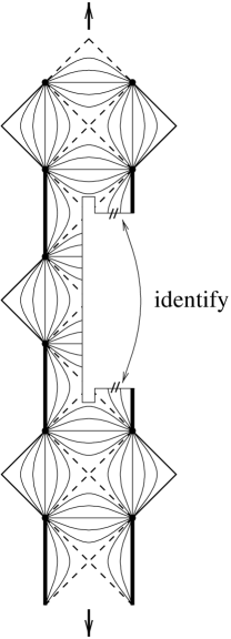
Figure 3.11: A possible RN-kink (cf. [267])

Such one, two or more dimensional lattices exhibit discrete symmetries, which, in turn, may be used to compactify manifolds by identifying certain curves. If this identification occurs in a nontrivial manner, “solitonic” manifolds are produced [267], as illustrated by the example Fig. 3.11.

3.3 Black hole in Minkowski, Rindler or de Sitter space

As a further illustration for the application of the methods described in this section a family of dilaton gravities [249] is considered which includes the physically most interesting models describing a single BH in Minkowski (cf. (2.33)), Rindler or de Sitter space. The potentials $U$ and $V$ are assumed to be of a simple monomial form,

$$U(X)=-\frac{a}{X}\,,\qquad V(X)=-\frac{B}{2}X^{a+b}.$$ (3.64)

Among the constants $a$, $b$ and $B$ only $a$ and $b$ distinguish between physically inequivalent models. $B$ plays the same role as $\lambda^{2}$ in (2.33), defining an overall scale factor.

In the line element (3.24) the functions $Q$ and $w$ read (cf. (3.12) and (3.15))

$$e^{Q(X)}=X^{-a}\,,\qquad w(X)=-\frac{B}{2(b+1)}X^{b+1}\,,$$ (3.65)

so that

$$(ds)^{2}=X^{-a}df\otimes\left[2dX+2\left(\mathcal{C}_{0}+\frac{B}{2(b+1)}X^{b+1}\right)\,df\right]\,.$$ (3.66)

The equation $w=\mathcal{C}_{0}$ has at most one solution on the positive semi-axis. Hence the metric (3.66) exhibits at most one horizon.

The most interesting models correspond to positive $a$ for which the function $X^{-a}$ diverges at $X=0$. For $X>0$ in terms of the alternative definition of the dilaton field $\Phi$ (2.11) the dilaton action (2.10) with the potentials (3.64) becomes

$$L^{\rm(dil)}=\frac{1}{2}\int d^{2}x\sqrt{-g}e^{-2\Phi}\left[R+4a(\nabla\Phi)^{2}-Be^{2(1-a-b)\Phi}\right]\,,$$ (3.67)

which may be more familiar to a string audience.

It is also instructive to calculate the scalar curvature:

$$R=2a\mathcal{C}_{0}X^{a-2}+\frac{Bb}{b+1}(b+1-a)X^{a+b-1}\,.$$ (3.68)

In what follows only models with $b\neq-1$ will be considered (although $b=-1$ can be analyzed too [249]). For the “ground state” solutions $\mathcal{C}_{0}=0$ only the second term in (3.68) survives. If $a=b+1$ or $b=0$ the scalar curvature of the ground state is zero. A more detailed analysis shows that the first case ($a=b+1$) corresponds to Minkowski space, and the second ($b=0$) to Rindler space. The condition $a=b+1$ for the Minkowski ground state models also follows from (3.40). If $a=1-b$ the ground state has constant curvature and corresponds to (anti-) de Sitter space.

For the general solutions (3.66) with $\mathcal{C}_{0}\neq 0$ it follows from (3.68) that, depending on the values of $a$ and $b$, they may show a curvature singularity at $X=0$, at $X=\infty$, or at both values. In the special cases considered above there could be only one singularity. Therefore, these models describe (in a somewhat generalized sense) a single BH immersed in Minkowski, or Rindler, or de Sitter space.

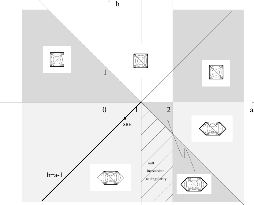
Figure 3.12: “Phase” diagram showing the CP diagrams related to the ($a$- and $b$-dependent) action (3.67). Bold lines in those diagrams denote geodesically incomplete boundaries. Spherically reduced models lie on the half-line $b=a-1$, $b\leq 0$, the endpoint of which corresponds to CGHS. The special case of SRG from $D=4$ is depicted by the point labelled by SBH.

Many interesting and important models belong to the two-parameter family of this section. The SRG models (2.2) for general dimension $D$ lie on the line $a=b+1$ between $a=1/2$ (this point corresponds to $D=4$) and $a=1$. As $D$ grows, these models approach the point $a=1$, corresponding to the CGHS model [71]. The point $a=0$, $b=1$ describes the Jackiw-Teitelboim model [22, 405, 238]. Lemos and Sa [298] gave the global solutions for $b=1-a$, Mignemi [323] considered $a=1$ and all values of $b$. The models of [148] correspond to $b=0$ and $a\leq 1$. The general solution for the whole plane was obtained in ref. [249] and is summarized in Fig. 3.12.

In order to calculate quantities like the ADM mass and the Hawking flux it is essential to re-write the line element (3.66) for asymptotically Minkowski, de Sitter and Rindler models in such a form that it becomes the standard one in the asymptotic region. Here we give an explicit expression for the asymptotically Minkowski solutions only (other cases can be found in ref. [299]) where such a representation is possible for $a\in(0,2)$. We repeat the steps which led before from the metric (3.24) to the Schwarzschild black hole (3.37). Namely, we first introduce the coordinates $\widetilde{X}=r,f=u$ (cf. (3.26))

$$u=\sqrt{\frac{B}{a}}\,f\,{\textrm{sign}}(1-a)\,,\qquad r=\sqrt{\frac{a}{B}}\frac{1}{|1-a|}X^{1-a}$$ (3.69)

and write the metric in EF form (3.27) where $\xi$ now reads

$$\xi\left(r\right)=2\mathcal{C}_{0}\left|1-a\right|^{\frac{a}{a-1}}r^{\frac{a}{a-1}}\left(\frac{B}{a}\right)^{\frac{2-a}{2\left(a-1\right)}}+1$$ (3.70)

Following the steps after (3.28) one arrives at the generalized Schwarzschild metric (3.34) with $\xi$ as in (3.70).

For $a\in(0,1)$ the asymptotic region corresponds to $r\rightarrow\infty$, while for $a\in(1,2)$ it is reached with the limit $r\rightarrow 0$. In both cases $\xi(r)\rightarrow 1$, and the metric assumes the standard Minkowski form $g_{\mu\nu}\rightarrow{\textrm{diag}}(1,-1)$.

For the asymptotically Rindler and de Sitter solution with $a$ belonging to the same interval, $a\in(0,2)$, the quantity $\xi$ becomes

$$\xi(r)=rB_{2}^{\frac{1}{2}}-Mr^{\frac{a}{a-1}}$$ (3.71)

for the Rindler solutions, and

$$\xi(r)=r^{2}B_{2}-Mr^{\frac{a}{a-1}}$$ (3.72)

for the de Sitter solutions. Explicit expressions for the constants $M$ and $B_{2}$ and for the variables $t$ and $r$ can be found in ref. [299]. The presence of typical linear (Rindler) and quadratic (de Sitter) terms in (3.71) and (3.72) should be noted.

Although the CGHS model $a=1$, $b=0$ belongs to the family of the asymptotically Minkowski models considered above, the equations (3.69) are singular at $a=1$. Appropriate coordinates for this case are

$$u=-\sqrt{B}f\,,\qquad r=-\frac{1}{\sqrt{B}}\ln{X}\,.$$ (3.73)

The line element (3.27) now contains

$$\xi(r)=1+\frac{2\mathcal{C}_{0}e^{\sqrt{B}r}}{B}\,.$$ (3.74)

A somewhat non-standard feature of (3.74) is that the asymptotic region is situated at $r\rightarrow-\infty$.

4 Additional fields

In $2D$ there are neither gravitons nor photons, i.e. no propagating physical modes exist [42]. This feature makes the inclusion of Yang-Mills fields in $2D$ dilaton gravity or an extension to supergravity straightforward. Indeed, both generalizations can be treated again as a PSM (2.34) with generalized $A_{I}$ and $X^{I}$. More locally conserved quantities (Casimir functions) may emerge and the integrability concept is extended.

Beside gauge fields also scalar and spinor fields may be added. If the latter are derived from higher dimensions through spherical reduction they are non-minimally coupled to the dilaton. The introduction of those fields in general destroys the integrability. Only in special cases exact solutions still can be obtained. An example are chiral fermions [278] or (anti-)selfdual scalars [356].

4.1 Dilaton-Yang-Mills Theory

The interaction with additional one-form Yang-Mills fields $A^{\underline{a}}$ related to local gauge transformations belonging to a compact Lie group $\mathcal{G}$ is simply included in (2.17) by introducing further auxiliary variables $Z^{\underline{a}}$ (additional target space coordinates in the PSM language) in the dilaton-Yang-Mills (DYM) action

$$L^{\rm(DYM)}=\int\limits_{\mathcal{M}_{2}}\,[\,X_{a}De^{a}+Xd\omega+Z^{\underline{a}}(\mathcal{D}A)^{\underline{a}}\\ +\epsilon\,\mathcal{V}(X^{a}X_{a},X,c_{1}(Z),c_{2}(Z),\;\ldots\;c_{n-1}(Z))\,]\,.$$ (4.1)

The gauge covariant derivative

$$(\mathcal{D}A)^{\underline{a}}=dA^{\underline{a}}+gf^{\underline{a}\underline{b}\underline{c}}\,A^{\underline{b}}A^{\underline{c}}$$ (4.2)

contains the structure constants $f^{\underline{a}\underline{b}\underline{c}}$ and the gauge coupling $g$. The potential $\mathcal{V}$, invariant under local Lorentz transformations and transformations $\mathcal{G}$ now also may depend on the Casimir invariants $c_{i}$ of the group $\mathcal{G}$. For instance in $\mathcal{G}=SU(N)$ there are $N-1$ independent invariant polynomials of degree $2,3,\,\ldots\,,N-1$ in terms of the components $Z^{\underline{a}}$.

The abelian case ($f=0$ in (4.2)) is especially simple. There $\mathcal{V}$ only depends on the single variable $Z$. Variation of (4.1) with respect to $A$ directly yields $dZ=0$, i.e. $Z=Z_{0}=\mbox{const}$ is conserved, an additional Casimir function in the PSM-interpretation of (4.1). Because $Z=Z_{0}$ is the result of solving a differential equation it cannot be simply reinserted into (4.1). Variation of $Z$ yields

$$dA=-\epsilon\left.\frac{\partial\mathcal{V}}{\partial Z}\;\right|_{Z=Z_{0}}\;.$$ (4.3)

The remaining e.o.m-s can be solved as for (2.17) by (3.20-3.23) with just an additional dependence on the constant $Z=Z_{0}$ in the potential $V$ in (3.22) and in $w(X,Z)$ of (3.23) [289, 305].

For a nonabelian gauge group $\mathcal{G}$ the coupling between the gauge fields $A^{\underline{a}}$ and the geometric variables is somewhat more complicated, but as a PSM it can be treated again along the lines of sect. 3.1. For a potential of the type $\mathcal{V}(X^{+}X^{-},X)+\alpha(X)Z^{\underline{a}}Z^{\underline{a}}$ the solution of the geometric sector can be obtained like the one from of an ordinary GDT, because $Z^{\underline{a}}Z^{\underline{a}}$ is constant on-shell [263, 264, 397]. Such a potential correctly reproduces the e.o.m.-s for ordinary D=2 dilaton-Yang-Mills theory:

$$(\mathcal{D}A)^{\underline{a}}=-\epsilon\alpha(X)Z^{\underline{a}}\,,\hskip 14.22636ptd(Z^{\underline{a}}Z^{\underline{a}})=0\,$$ (4.4)

Some explicit solutions for the dilaton-Maxwell-Scalar system can be found in ref. [353].

The action (4.1) does not contain the special case which emerges from spherical reduction of Einstein-Yang-Mills (EYM) in $D=4$. The reason for this is obvious: While the Killing vectors $\xi_{s}$ associated with spherical symmetry act trivially on the metric, $\delta_{\xi_{s}}g_{\mu\nu}=0$ with $\delta_{\xi_{s}}$ being the Lie-derivative with respect to $\xi_{s}$, a corresponding transformation of the gauge field $A_{\mu}\to A_{\mu}-\varepsilon^{s}\delta_{\xi_{s}}A_{\mu}$ can be compensated by a suitable gauge transformation, $A_{\mu}\to A_{\mu}+\varepsilon^{s}\mathcal{D}_{\mu}W_{s}$, such that $\delta_{\xi_{s}}A_{\mu}=\mathcal{D}_{\mu}W_{s}$ [162]. Already for $SU(2)$ the most general solution compatible with spherical symmetry, sometimes called “Witten’s ansatz” [438], yields terms which are not described by (4.1), namely an additional (minimally coupled) charged scalar field with dilaton-dependent mass term and quartic self-interaction.

4.2 Dilaton Supergravity

Already a long time ago the superfield approach has been applied in supersymmetric extensions of GDTs [223]. Superfields are expressed in terms of supercoordinates $z^{M}=(x^{m},\theta^{\mu})$, where the bosonic coordinates $x^{m}$ are supplemented by anticommuting (Grassmann) coordinates $\theta^{\mu}$.

We assume the latter to be Majorana spinors, i.e. we restrict ourselves to $N=1$ superspace in $D=2$. Beside the $\mathbb{Z}_{2}$-grading property for coordinates,

$$z^{M}z^{N}=(-1)^{MN}z^{N}z^{M}\,,$$ (4.5)

the derivatives with respect to $z$ are defined to act to the right $\overset{\,\raisebox{-2.15277pt}{$\scriptscriptstyle\rightarrow$}}{\partial}{}_{M}=\overset{\,\raisebox{-2.15277pt}{$\scriptscriptstyle\rightarrow$}}{\partial}{}/\partial z^{M}$. Only those derivatives will appear in the following, so the arrow will be dropped.

Any vector-field in superspace $V=V^{M}\partial_{M}$ is invariant under non-degenerate coordinate changes $z^{M}\to\bar{z}^{M}(z)$

$$V^{M}\partial_{M}=\bar{V}^{M}\;\frac{\partial z^{L}}{\partial\bar{z}^{M}}\;\frac{\partial\bar{z}^{N}}{\partial z^{L}}\;\frac{\partial}{\partial\bar{z}^{N}}\,,$$ (4.6)

which shows the advantage of the conventional summation of indices “ten to four” in supersymmetry, already introduced in the section on PSM-s (sect. 2.3).

Now any formula of differential geometry in ordinary space of the PSM can be copied to superspace notation. The p-forms eq. (1.14), of sect. 1.2.1 turn into the same expressions written in terms of $dz^{M}$ instead of $dx^{\mu}$, adhering strictly to the summation of supersymmetry:

$$\Phi=\frac{1}{p!}dz^{M_{p}}\wedge\cdots\wedge dz^{M_{1}}\Phi_{M_{1}\cdots M_{p}}$$ (4.7)

Also the external differential is defined in agreement with sect. 2.3 as

$$d\Phi=\frac{1}{p!}dz^{M_{p}}\wedge\cdots\wedge dz^{M_{1}}\wedge dz^{N}\partial_{N}\Phi_{M_{1}\cdots M_{p}}$$ (4.8)

which implies the Leibniz rule (2.37) for superforms, already introduced in that section in anticipation of the graded PSM (gPSM) approach below. Clearly the (anti-)symmetry properties of the tensor $\Omega_{M_{1}\,\ldots\,M_{p}}$ now depend on the graded commutation properties (4.5) of the indices. Instead of (1.13), (1.14) the one-forms of superzweibein and superconnection are $E_{M}{}^{A}$ and

$$\Omega_{MA}{}^{B}=\Omega_{M}L_{A}{}^{B}\,,$$ (4.9)

where in (4.9) the simplification for two dimensions with

$$L_{A}{}^{B}=\left(\begin{array}[]{cc}\epsilon_{a}{}^{b}&0\\ 0&-\frac{1}{2}(\gamma_{\ast})\!{}_{\alpha}{}^{\beta}\end{array}\right)$$ (4.10)

already has been taken into account. The fermionic part in (4.10), the generator of Lorentz transformations in spinor space, agrees with (1.61). Covariant derivatives, defined by analogy to (1.23)

$$\begin{split}\nabla_{M}V^{A}&=\partial_{M}V^{A}+\Omega_{M}V^{B}L_{B}{}^{A}\,,\\ \nabla_{M}V_{A}&=\partial_{M}V_{A}-\Omega_{M}L_{A}{}^{B}V_{B}\;.\end{split}$$ (4.11)

lead to the expressions for the components of supercurvature and supertorsion

$$R_{MNA}{}^{B}=\left(\partial_{M}\Omega_{N}-\partial_{N}\Omega_{M}(-1)^{MN}\right)L_{A}{}^{B}=:F_{MN}L_{A}{}^{B},$$ (4.12)

$$T_{MN}{}^{A}=\partial_{M}E_{N}{}^{A}+\Omega_{M}E_{N}{}^{B}\Omega_{M}L_{B}{}^{B}-(M\leftrightarrow N)(-1)^{MN}$$ (4.13)

Again Bianchi identities, direct generalizations of (1.26) and (1.28), must hold (cf. [142], eqs. (1.58), (2.20)). They restrict the component fields, contained in $E_{M}{}^{A},\Omega_{M}$ when these expressions are expanded in terms of (a finite number of) ordinary fields, appearing as coefficients of powers $\Theta^{\mu}$ and $\Theta^{2}=\Theta^{\mu}\Theta_{\mu}$. It turns out that to deal with supertorsion it is more convenient to use its anholonomic components:

$$T_{AB}{}^{C}=(-1)^{A(B+N)}\,E_{B}{}^{N}E_{A}{}^{M}T_{MN}{}^{C}$$ (4.14)

The literature on $2D$ supergravity (cf. e.g. [223, 60, 315, 370, 368, 297]) is strongly influenced by its close relation to string theory, where the bosonic torsion vanishes, $T_{ab}{}^{c}=0$. It uses the further constraints on $T_{AB}{}^{C}$

$$T_{\alpha\beta}{}^{c}=2i\,(\gamma^{c})_{\alpha\beta},\qquad T_{\alpha\beta}{}^{\gamma}=0\,,$$ (4.15)

the first of which is dictated by the requirement that in the limit of global transformations ordinary supersymmetry should be restored. The second one turns out to be a convenient choice, because then the Bianchi identities in a Wess-Zumino type gauge are fulfilled identically [141].

In the application to $2D$ gravity including bosonic torsion it seems natural to retain (4.15), but to simply drop the zero bosonic torsion condition. However, as a consequence of the Bianchi identities it turned out [141] that the superfield components, obtained in this manner, did not permit the construction of $2D$ supergravity Lagrangians with nonvanishing bosonic torsion, after all. Only after replacing (4.15) by the weaker set ($F_{\alpha\beta}=E_{\alpha}{}^{M}\,E_{\beta}{}^{N}\,F_{NM}(-1)^{M}$, cf. (4.12))

$$(\gamma_{a})^{\beta\alpha}\,T_{\alpha\beta}{}^{c}=-4i\delta_{a}{}^{c},\quad T_{\alpha\beta}{}^{\gamma}=0,\quad(\gamma_{a})^{\beta\alpha}F_{\alpha\beta}=0$$ (4.16)

a solution can be found [142]. However, the mathematical complexity of this approach becomes considerable.

Instead, we turn to the generalization of the PSM, adding fermionic target space coordinates $\chi^{\alpha}$ and corresponding Rarita-Schwinger 1-form fields $\psi_{\alpha}$ to the degrees of freedom in (2.34), (2.38) as

$$\begin{split}X^{I}&=(X,X^{a},\chi^{\alpha})\,,\\ A_{I}&=(\omega,e_{a},\psi_{\alpha})\;.\end{split}$$ (4.17)

Apart from that, the PSM action retains the form (eq. (2.34)).

Both $\chi^{\alpha}$ and $\psi_{\alpha}$ denote Majorana fields, when, as in what follows, $N=1$ supergravity is considered. The graded Poisson tensor $\mathcal{P}^{IJ}=(-1)^{IJ+1}\mathcal{P}^{JI}$ instead of (eq. (2.36)) is now assumed to fulfill a graded Jacobi identity

$$\mathcal{P}^{IL}\overset{\,\raisebox{-2.15277pt}{$\scriptscriptstyle\rightarrow$}}{\partial}{}_{L}\mathcal{P}^{JK}+\operatorname{gcycl}(IJK)=0\,.$$ (4.18)

Except for the range of fields to be summed over, the e.o.m-s are again (2.41), (2.42). The symmetries (2.43), (2.44) depend on infinitesimal local parameters $\epsilon_{I}=(\epsilon_{\phi},\epsilon_{a},\epsilon_{\alpha})$.

The mixed components $\mathcal{P}^{\alpha X}$ are constructed by analogy to $\mathcal{P}^{aX}$ in (2.39) with the appropriate generator $(-\gamma_{\ast}/2)$ of Lorentz transformations in $2D$ spinor space (cf. eq. (4.10)). Then $d\epsilon_{\alpha}$ in the second set of eq. (2.44) acquires an additional term casting it into the covariant combination $(D\epsilon)_{\alpha}$, with covariant derivative (1.63). This is precisely the form required for the (dilaton deformed) supergravity transformation of the “gravitino” $\psi_{\alpha}$. As the Poisson tensor $\mathcal{P}^{IJ}$ also here is not of full rank, Casimir functions $\mathcal{C}(Y,\phi,\chi^{2})$ exist which, following the same line of argument as in sect. 2.3 obey $d\mathcal{C}=0$. From Lorentz invariance a bosonic $\mathcal{C}$ in supergravity is of the form

$$\mathcal{C}=c+{\textstyle\frac{1}{2}}\chi^{2}c_{2}\,,$$ (4.19)

where $c$ coincides with the quantity denoted by $\mathcal{C}$ in the pure bosonic case (2.46,3.23). However, also fermionic Casimir functions may appear (see below).

The determination of all possible minimally extended supergravities reduces to the solution of the Jacobi identities (4.18). In the general ansatz for $\mathcal{P}^{IJ}$

$$\mathcal{P}^{ab} =V\,\epsilon^{ab}\,,$$ (4.20)

$$\mathcal{P}^{b\phi} =X^{a}\,\epsilon_{a}{}^{b}\,,$$ (4.21)

$$\mathcal{P}^{\alpha\phi} =-\frac{1}{2}\chi^{\beta}(\gamma_{\ast})_{\beta}{}^{\alpha}\,,$$ (4.22)

$$\mathcal{P}^{\alpha b} =\chi^{\beta}(F^{b})_{\beta}{}^{\alpha}\,,$$ (4.23)

$$\mathcal{P}^{\alpha\beta} =v^{\alpha\beta}+\frac{\chi^{2}}{2}\,v_{2}^{\alpha\beta}\,,$$ (4.24)

the function

$$V=\mathcal{V}(X,Y)+\frac{\chi^{2}}{2}\,v_{2}(X,Y)$$ (4.25)

contains the original bosonic potential $\mathcal{V}$. As explained above, eqs. (4.21) and (4.22) are fixed completely by Lorentz invariance. This invariance also implies that the (symmetric) spinor-tensor $V^{\alpha\beta}$ in (4.24) can be expanded further into three scalar functions of $X$ and $Y$, multiplying the symmetric matrices $(\gamma_{\ast})^{\alpha\beta},\gamma_{a}^{\alpha\beta},X^{a}(\gamma_{\ast}\gamma_{a})^{\alpha\beta}$:

$$\begin{split}V^{\alpha\beta}&=\mathcal{U}\gamma_{\ast}{}^{\alpha\beta}+i\,\widetilde{\mathcal{U}}X^{a}\gamma_{a}{}^{\alpha\beta}+i\,\widehat{\mathcal{U}}X^{a}\epsilon_{a}{}^{b}\gamma_{b}{}^{\alpha\beta}=\\ &=v^{\alpha\beta}+\frac{\chi^{2}}{2}v_{2}^{\alpha\beta}\;.\end{split}$$ (4.26)

Each function $\mathcal{U}$ again has a pure bosonic part and, as indicated in the second line of (4.26), a term proportional to $\chi^{2}$. In a similar manner the spinor $F^{b}$ in (4.23) can be expressed in terms proportional to $\delta_{\beta}{}^{\alpha},(\gamma^{a})_{\beta}{}^{\alpha}(\gamma_{\ast})_{\beta}{}^{\alpha}$ which finally requires eight scalar functions of $X$ and $Y$, multiplied by appropriate factors constructed with the help of $X^{a}$ and $\epsilon^{ab}$ [140]. In (4.23) the multiplying factor $\chi$ precludes terms with factor $\chi^{2}$ in $F$. Thanks to (4.21) and (4.22) the Jacobi identities with one index referring to $X$ are fulfilled automatically. The remaining ones can be solved algebraically, provided a quite specific sequence of steps is followed (for details see [140]). Three main cases are determined by the rank of the $2\times 2$ spinor matrix $v^{\alpha\beta}$ in (4.26).

For full rank ($\det\,v^{\alpha\beta}\neq 0$) the solution is found to depend on five scalar functions of $X,Y$ and the derivatives thereof, if the bosonic potential $\mathcal{V}$ in (4.25) is assumed to be given.

If the fermionic rank is reduced, beside the bosonic Casimir function (4.19) one or two fermionic ones exists. They are of the generic form

$$\mathcal{C}^{(\pm)}=\chi^{\pm}\;\left|\,\frac{X^{--}}{X^{++}}\,\right|^{\pm 1/4}\;c_{(\pm)}\,(X,Y)$$ (4.27)

and owe their Lorentz invariance to the interplay of the abelian boost transformations $\exp(\pm\beta)$ of the light cone coordinates $X^{\pm\pm}$ related to $X^{a}$, and $\exp(\pm\beta/2)$ of the chiral spinor components $\chi^{\pm}$ of $\chi^{\alpha}$. For fermionic rank 1 the general solution contains four arbitrary functions beside $\mathcal{V}$ and one additional Casimir function of type (4.27). For rank zero of the fermionic extension in $\mathcal{P}^{IJ}$ beside (4.19) both fermionic Casimir functions (4.27) are conserved and three functions remain arbitrary for a given bosonic potential.

In order to avoid solving differential equations by imposing the Jacobi identities (4.18) also for reduced fermionic rank, it is important to make intensive use of the information on the Casimir functions.

The arbitrariness of the solution of the Jacobi identities can be understood as well by studying reparametrizations of the target space, spanned by the $X^{I}$ in the gPSM. Those reparametrizations may generate new models. Therefore, they can be useful to create a more general gPSM from a simpler one, although this approach is difficult to handle if $\mathcal{V}$ in (4.25) is assumed to be the given starting point. However, the subset of those reparametrizations may be analyzed which leaves a given bosonic theory unchanged. Again the same number of arbitrary functions emerges for the different cases described in the paragraphs above.

As an illustration we quote eq. (4.252) from [140] which represents one (of many) supergravity actions which possess a bosonic potential (2.31) quadratic in torsion:

$$\begin{split}L^{\rm(QBT)}&=\int_{\mathcal{M}}Xd\omega+X^{a}De_{a}+\chi^{\alpha}D\psi_{\alpha}+\epsilon\left(V+{\textstyle\frac{1}{2}}X^{a}X_{a}U+{\textstyle\frac{1}{2}}\chi^{2}v_{2}\right)\\ &+\frac{U}{4}X^{a}(\chi\gamma^{3}\gamma_{a}\gamma^{b}e_{b}\psi)-\frac{i\,V}{2u}(\chi\gamma^{a}e_{a}\psi)\\ &-\frac{i}{2}X^{a}(\psi\gamma_{a}\psi)-\frac{1}{2}\left(u+\frac{U}{8}\chi^{2}\right)(\psi\gamma^{3}\psi),\\ v_{2}&=-\frac{1}{2u}\left(VU+V^{\prime}+\frac{V^{2}}{u^{2}}\right).\end{split}$$ (4.28)

In this formula $U(X)$ is the quantity defined in (2.31). The prepotential $u$ is related to $U(X)$ and $V(X)$ by

$$u^{2}(X)=-2\,e^{-Q(X)}\,w(X)\,,$$ (4.29)

where $Q$ and $w$ have been defined in (3.12) and (3.15).

The supergravity transformations of $e_{a}$ and $\psi_{\alpha}$ with small fermionic parameter $\epsilon$ for this action (4.28)(cf. eqs. (4.255) - (4.259) of [140] and footnote 38) are of the form

$$\delta\,e_{a}=i\,(\epsilon\gamma_{a}\psi)+\cdots,\hskip 14.22636pt\delta\,\psi_{\alpha}=-(D\,\epsilon)_{\alpha}+\cdots\;.$$ (4.30)

Thus, they contain the essential terms, but, not shown here, also others, because of the deformation by the dilaton field. SRG is the special case (2.33) for $U$ and $V$, but as a supergravity extension (4.28) is not unique.

A generic property of the fermionic extensions obtained in this analysis is the appearance of obstructions, which is a typical feature of supersymmetric theories (cf. e.g. [133]). The first type of those consists in singular functions of the bosonic variables $X$ and $Y$, multiplying the fermionic parts of a supergravity action, when no such singularities are present in the bosonic part. But even in the absence of such additional singularities, a relation like (4.29) between the original potential and some prepotential $u$, dictated by the corresponding supergravity theory, either leads to a restriction of the range of $X$ and/or $Y$ as given by the original bosonic one, or even altogether prevents any extension of the latter. Remarkably, a known $2D$ supergravity model like the one of Howe [223] which originally had been constructed with the full machinery of the superfield technique, is one example which escapes such obstructions. There, in our language, the PSM potential $\mathcal{V}=-2\lambda^{2}X^{3}$ permits an expansion in terms of the prepotential $u(X)$ through $\mathcal{V}=-du^{2}/dX$ because $Q=0$. An example where obstructions seem to be inevitable is the KV-model [250] with quadratic bosonic torsion.

On the other hand, the supergravity extension of SRG following from the action (4.28) is free from such problems. However, it is not the only possible extension of the bosonic theory. Indeed, the hope that a link could be found between the possibility of reducing the arbitrariness of extensions referred to above, and of the absence of such obstructions, did not materialize. Several counter examples could be given including different singular and nonsingular extensions of SRG.

Another very important point concerns the “triviality” of supergravity extensions, proved earlier by Strobl [398]. It was based upon the observation that locally a formulation of the dynamics in terms of Darboux coordinates allows to elevate the infinitesimal transformations (2.43,2.44) (on-shell) to finite ones. Then the latter may be used to gauge the fermionic fields in $2D$ supergravity to zero. Providing now the explicit form of those Darboux coordinates in the explicit solution of a generic model, additional support has been given to the original argument of ref. [398]. However, the appearance of the obstructions and the ensuing singular factors in the transition to the Darboux coordinates may introduce a new aspect. When those new singularities appear at isolated points without restriction of the range for the original bosonic field variable, they may be interpreted and discarded much like coordinate singularities. Another way to circumvent this problem in the presence of restrictions to the range and thus to retain triviality is to allow a continuation of our (real) theory to complex variables. This triviality disappears anyhow, when interactions with additional matter fields are introduced, obeying the same symmetry as given by the gPSM-theory. A proposal in this direction can be found in ref. [237].

In order to eliminate the arbitrariness of superdilaton extensions the only viable argument seems to start from a supergravity theory in higher dimensions (e.g. $D=4$) and to reduce it (spherically or toroidally) to a $D=2$ effective theory. It turns out that the Killing spinors needed in that case must be Dirac spinors, requiring the generalization of the work of ref. [140] to (at least) $N=2$, where, however, the same technique of gPSM-s can be applied.

As in the bosonic case an action like (4.28) or, better, directly its gPSM form (2.34) can be converted into a dilaton theory by elimination of the torsion dependent part of the spin connection and of $X^{a}$. Also for supergravity the equation for $X^{a}$ is independent of the potential $\mathcal{V}$, eq. (2.29) being replaced by

$$X^{a}=-e^{a}_{m}\epsilon^{mn}[(\partial_{n}X)+\frac{1}{2}(\chi\gamma_{\ast}\psi_{n})]\;.$$ (4.31)

The corresponding dilaton action in the gPSM notation becomes

$$L=\int\limits_{\mathcal{M}}[Xd\tilde{\omega}+\chi^{\alpha}(D\psi)_{\alpha}+\frac{1}{2}\mathcal{P}^{AB}\,|_{X^{a}}\,e_{B}\,e_{A}\,]\,,$$ (4.32)

where $\tilde{\omega}$ is the torsionless part of the curvature as in (2.27) and $|_{X^{a}}$ means that the components of the Poisson tensor (in the anholonomic basis) are to be taken with $X^{a}$ given by (4.31). When (4.32) is written in components (cf. eq. (4.246) of [140]) with the bosonic potential (2.31) for the Howe model ($V=-\frac{1}{2}X^{3},U=0$), it can be checked that the superdilaton theory, obtained in this way differs from the direct superextension of the bosonic theory [354]. The reason is that in our approach $X$ is directly promoted to be the bosonic component of the superfield, whereas in ref. [354] the dilaton represents the bosonic part of yet another scalar superfield.

4.3 Dilaton gravity with matter

4.3.1 Scalar and fermionic matter, quintessence

For the inclusion of scalar matter as in sect. 2.1 we start with the example of spherical reduction of Einstein theory. When massless scalar fields are coupled minimally in $D$ dimensions ($(\nabla_{(D)}\Phi)^{2}=g^{MN}\partial_{M}\Phi\,\partial_{N}\Phi$ ; $M,N=0,1,\ldots\,D-1$)

$$L^{(m,D)}_{(\phi)}=\frac{1}{2}\,\int d^{D}x\,\sqrt{-g_{(D)}}\;(\nabla_{(D)}\Phi)^{2}\,,$$ (4.33)

for scalar fields $\phi=\phi(x^{0},x^{1})$ the $2D$ reduced action in terms of the components of $g^{MN}$ as derived from the line-element (2.1), becomes

$$L^{(m)}_{(\phi)} =\frac{\mathcal{O}_{D-2}}{\,\lambda^{D-2}}\;\int d^{2}x\sqrt{-g}\,F(X)\,(\nabla\phi)^{2}\,,$$ (4.34)

$$F_{SRG}(X) =\frac{X}{2}\;.$$ (4.35)

Such an interaction is an example of nonminimal coupling ($F(X)\neq\rm const$.) in the reduced case. Admitting a general function $F(X)$, a dilaton field dependence different from SRG (eq. (4.35)) can be covered as well. An especially simple theory follows for $F={\rm const.}$, minimal coupling at the $D=2$ level. Below we shall absorb the relative factor $1/2$ between the dilaton action (2.2) and the first order action (2.17) – which of course must also be adjusted properly in the matter action – into the coupling function $F(X)$.

Dropping as in our convention for the geometrical part of the FOG action in (2.17) the prefactor $2\mathcal{O}_{D-2}/\lambda^{D-2}$, the action (4.34) can be written also as

$$L^{(m)}_{(\phi)}=\frac{1}{2}\;\int\limits_{\mathcal{M}_{2}}\;F\,d\phi\ast d\phi=\frac{1}{2}\;\int F\,(d\phi e^{a})\ast(d\phi e^{b})\,\eta_{ab}\;.$$ (4.36)

In order to avoid the delicate subject of Killing spinors, necessary for the (spherical) reduction of fermions (cf. e.g. [358] for $D=4$) we shall only deal with fermions introduced directly in $D=2$. The diffeomorphism covariant generalization (cf. (1.63)) of the Dirac action

$$L^{(m)}_{(\psi)}=\frac{i}{4}\;\int d^{2}x\,\sqrt{-g}\;e^{\mu}_{a}\,(\bar{\psi}\gamma^{a}\overset{\leftrightarrow}{D}_{\mu}^{(\psi)}\,\psi)$$ (4.37)

as in Minkowski space must contain a two-sided derivative $a\overset{\leftrightarrow}{D}b=a(Db)-(Da)b$ in order to yield a real action. The cancellation of $\omega$ in that derivative is a peculiar feature of $D=2$, i.e. the simplification $\overset{\leftrightarrow}{D}_{\mu}=\overset{\leftrightarrow}{\partial}_{\mu}$ is possible there. Thus both interactions (4.36) and (4.37) do not depend on the spin connection, as anticipated already in deriving the (classical) e.o.m.-s with matter, eqs. (3.6)-(3.10).

An additional geometrical degree of freedom may also appear already at the $D=4$ level. Recently in connection with the observation of supernovae at high values of the redshift [367, 365, 366, 359] the validity of the Hilbert-Einstein theory has been put into doubt [12]. The simplest theoretical description requires the introduction of a (still very small) cosmological constant $\Lambda$ (de Sitter theory). Therefore, extensions of the Einstein theory towards the old Jordan-Brans-Dicke (JBD) theory [153, 241, 51], have been revived, where already at $D=4$ an additional scalar field $\Phi$ (Jordan field, “quintessence”) is assumed to exist [433, 431, 80, 447, 363]. Then, already in $D=4$ an action like (2.9) is postulated with $X\to\Phi$ and appropriate assumptions for functions $U_{(4)}(\Phi),V_{(4)}(\Phi)$ so that the “effective cosmological constant” is driven to its present (small) value

$$L^{\rm(Q)}=\int d^{4}x\,\sqrt{-g_{(4)}}\;\left[R_{(4)}\,\Phi+U_{(4)}(\Phi)\,(\nabla_{(4)}\Phi)^{2}\,+V_{(4)}(\Phi)\;\right]\;.$$ (4.38)

After spherical reduction of (4.38), even without including a genuine matter interaction a $2D$ theory emerges where the (in $D=4$ geometric) variable $\Phi$ turns into something like an additional scalar field (beside the genuine $D=2$ dilaton field $X$). These “two-dilaton theories” have been studied in more detail in [194]. The most interesting feature of such theories is that one dilaton field plays the role of a “geometric” dilaton field in $D=2$ and the other one behaves like matter, providing continuous physical degrees of freedom. We shall discuss the classical and quantum properties of dilaton gravity with (4.34), (4.35) in sect. 7.

4.3.2 Exact solutions – conservation law for geometry and matter

In the presence of interactions with additional fields which – in contrast to gauge fields (cf. subsection 4.1) or supergravity (subsection 4.2) – cannot be incorporated into the PSM approach, the possibility to find analytic solutions is restricted. Nevertheless, the interest in such solutions had been raised, especially by the work on the CGHS model (cf. sect. 2.1.2). It possesses a global structure very much like the one of the genuine Schwarzschild BH (Fig. 3.8). Also application of the (singular) dilaton field dependent conformal transformation (1.56) with dilaton dependent conformal factor

$$\rho_{CGHS}=-\frac{1}{2}\int^{X}U_{CGHS}(X^{\prime})dX^{\prime}=\frac{1}{2}\ln{X}$$ (4.39)

is found to cancel the torsion term (cf. sect. 2.1.4). The transformed potentials read

$$\tilde{U}(X)=0,\hskip 14.22636pt\tilde{V}(X)=V_{CGHS}(X)e^{Q_{CGHS}(X)}=\rm const.$$ (4.40)

Then also the action for the scalar field (4.36) becomes the one in a flat background ($g_{\mu\nu}\to\eta_{\mu\nu}$). In this model $F$ is taken to be constant (minimal coupling). After (trivially) solving for the (free) scalar or fermionic fields, the inverse conformal transformation is applied. This method has also been extended to include one-loop quantum effects in the semi-classical approach, by describing that lowest order quantum effect through the Polyakov effective action [361]. Adding to this action another piece, adapted suitably so that the exact solubility is maintained, more semi-classical solutions have been studied [374, 44, 115, 147, 256, 446, 445]. An approximate analysis of the solutions is possible, of course, for a larger class of models. For instance, it has been demonstrated [252] that adding the Polyakov term to SRG shifts and attenuates the BH singularity.

In the exact solution without matter, the important step has been to use one of the eqs. (3.8) to express $\omega$ as in (3.16). If the theory only depends on one type of chiral fields either $W^{-}$ or $W^{+}$ in (3.8) vanishes. Then the same elimination of $\omega$ can be used. Separating e.g. Dirac fermions into chiral components as

$$\Psi=\sqrt[4]{2}\,\left(\begin{array}[]{c}\chi_{R}\\ \chi_{L}\end{array}\right)\,,\quad\bar{\Psi}=\sqrt[4]{2}\;\left(\chi_{R}^{\dagger},\chi_{L}^{\dagger}\right)\,,$$ (4.41)

the interaction (4.37) may be written as

$$L^{(m)}_{(\Psi)} =-\int\limits_{\mathcal{M}_{2}}\,(e^{+}J^{-}+e^{-}J^{+})\,,$$ (4.42)

$$J^{-,+}=J^{R,L} =i\,\left[\chi^{\dagger}_{R,L}\,(d\chi_{R,L})-(d\chi^{\dagger}_{R,L})\,\chi_{R,L}\;\right]\;.$$ (4.43)

Also “amplitudes” $k$ and “phases” $\varphi$ can be introduced,

$$\chi_{R,L}=\frac{1}{\sqrt{2}}\,k_{R,L}\,e^{i\varphi_{R,L}}\,,$$ (4.44)

in terms of which the chiral currents (4.43) become

$$J^{+,-}=-k^{2}_{L,R}\,d\varphi_{L,R}\;.$$ (4.45)

Since the theory only depends upon one type of chiral fields, either $J^{+}$ or $J^{-}$ in (4.42) is zero [278, 356]. Still an equation like (3.16) without matter contribution holds, and the further steps of the solution for the geometric variables are exactly as in the matterless situation, except for the matter contribution in the conservation law. The general case from (3.8) and (3.7) may be derived from

$$d(X^{+}X^{-})+\mathcal{V}(X,Y)\,dX+X^{-}W^{+}+X^{+}W^{-}=0\;.$$ (4.46)

For chiral fermions only one of the two last terms remains. As the consequences of (4.46) are of more general importance we will come back to that relation when the situation without restrictions on matter will be discussed below.

The matter equation for chiral fermions $k_{L}=0$ in (4.44) by variation of $\varphi_{R}$ and $k^{2}_{R}$

$$e^{+}d\,\varphi_{R}=0\,,$$ (4.47)

$$d\,(k^{2}_{R}\,e^{+})=0$$ (4.48)

are solved easily, because $e^{+}$ is the previous solution (3.20). Eq. (4.47) implies that $\varphi_{R}=\varphi_{R}\,(f)$ where $f$ is the arbitrary function introduced in (3.20). Inserting the latter into (4.48) determines the amplitude:

$$k_{R}^{2}=\frac{e^{-Q(X)}}{X^{+}}\;g(f)$$ (4.49)

An analogous procedure works for chiral scalars. Variation with respect to $e^{\mp}$ of the action (4.36) for $F=\mbox{const.}$ in light-like coordinates ($\phi^{\pm}=\ast(d\phi e^{\pm})$) yields

$$W^{\pm}=-F\left[\phi^{\pm}\,d\phi\mp e^{\pm}\phi^{+}\phi^{-}\right]\,,$$ (4.50)

so that for (anti-)selfdual scalars with either $\phi^{+}=0$ (selfdual: $\ast d\phi=d\phi$) or $\phi^{-}=0$ (anti-selfdual: $\ast d\phi=-d\phi$) again one of the eqs. (3.8) is independent of the matter contribution. The subsequent steps to obtain the exact solution proceed as for chiral fermions.

The e.o.m. for minimally coupled scalars can be written as

$$d\ast d\phi=d(\phi^{-}e^{+})=d(\phi^{+}e^{-})=0$$ (4.51)

where the last two forms are to be used, respectively, in the (anti-)selfdual cases. Thus (anti-)selfdual matter identically solves (4.51). Furthermore, e.g. for selfdual $\phi$ the condition $e^{+}d\phi=0$ makes the lines of $\phi=\mbox{const.}$ light-like. With the same solution (3.20) for $e^{+}$ as without matter, the latter relation leads to $d\phi df=0$, i.e. $\phi=\phi(f)$, or vice versa. As $f$ represented a null coordinate in the EF line element, the peculiar light-like nature of $\phi$ is confirmed. The similarity between (anti-)selfdual scalars and chiral fermions is not surprising in view of the well-known close relation between scalars and fermions in $D=2$ [439].

Other nontrivial examples of exactly soluble systems are static solutions [159] or continuously self-similar solutions [369] of SRG with a massless (non-minimally coupled) scalar field.

Minimally coupled scalars with SRG for the geometric sector can be solved in a perturbative manner [329] or in the static limit [177, 176].

With the exception of aforementioned special cases, the CGHS model, the models of refs. [154, 155] or some other simple potentials like e.g. constant $V$ (i.e. Rindler metric) and of teleparallelism (pure torsion, $V=0$) [410] no exact solution with general (scalar or fermionic) matter seems to be known. Indeed, one of the main open problems in classical dilaton theory with matter is an analytic (as opposed to numerical) description of non-trivial systems showing the feature of critical collapse.

5 Energy considerations

It is important to clarify the relation of certain quantities appearing in generic $D=2$ gravity theories (like the absolutely conserved quantity $\mathcal{C}^{\left(g\right)}$) with respect to corresponding concepts well-known from $D=4$ Einstein gravity.

5.1 ADM mass and quasilocal energy

Because of diffeomorphism invariance the Hamiltonian density vanishes on the surface of the constraints in all gravity theories including all $2D$ dilaton models. However, a boundary term must be included in the Hamiltonian which can be used to define a global or “quasilocal” energy. This is the essence of the Arnowitt–Deser–Misner procedure [7]. As discussed in detail by Faddeev [149] in the context of $4D$ Einstein gravity, this boundary is the one at (spatial) infinity, and the value of the gravitational energy is very sensitive to the choice of asymptotic conditions and it is not invariant under the change of coordinates at infinity. This reflects the fact that the energy is related to an observer connected with the asymptotic coordinate system who measures this energy. In generic $2D$ dilaton gravity the situation becomes even more complicated since a natural asymptotic coordinate system does not exist for some of the models. This lack of asymptotic diffeomorphism invariance (and of conformal invariance) has led to much confusion in the literature.

To facilitate comparison with other works on the ADM approach we consider here the second order dilaton action (3.67) with the exponential parameterization $X=e^{-2\Phi}$ for the dilaton field. Since only the first term $e^{-2\Phi}R$ is essential for the calculation of the ADM mass, this does not imply any restrictions on the potentials $U$ and $V$.

The diagonal gauge for the metric ($N=\sqrt{\xi}\dot{f},\Lambda=\sqrt{\xi}f^{\prime}$ in (3.33))

$$(ds)^{2}=N^{2}(dt)^{2}-\Lambda^{2}(dr)^{2}\,.$$ (5.1)

is sufficient for our purposes since the lapse $N$ is a Lagrange multiplier for the Hamiltonian constraint in generally covariant theories. A more complete canonical analysis can be found in refs. [276, 307, 295, 280, 299].

The next step is to supplement the volume action (3.67) by a suitable boundary term. The role of the latter is to convert second order derivatives to first order ones. More exactly, such a term must provide standard variation equations for the boundary data, the induced metric on the boundary. In particular, this means that the first variation of the total action must not contain boundary contributions with normal derivative for the variation of the lapse $N$. Since only the curvature term contains second derivatives, it also must not depend on the potentials $U$ and $V$ in (2.9). Therefore, we may adopt for all models the expression for the SRG model. It can be obtained by spherical reduction of the standard extrinsic curvature term in four dimensions. This yields

$$L^{b}=\int\limits_{\partial\mathcal{M}}Ndt\,e^{-2\Phi}K\,,$$ (5.2)

where we assume that $\partial\mathcal{M}$ corresponds to a constant value of $r$. $N\,dt$ is the surface element on the boundary, $e^{-2\Phi}$ is produced by the spherical reduction. $K$ is the extrinsic curvature,

$$K=-\frac{1}{N}\partial_{n}N=\mp\frac{1}{\Lambda}\partial_{r}(\log N)\,,$$ (5.3)

where $\partial_{n}$ denotes the derivative with respect to an outward pointing unit normal. The upper (lower) sign in (5.3) should be taken on the “right” (“left”) component of the boundary.

For linear variations around a static background in the diagonal gauge (3.33) the curvature follows from the simplified formula

$$\sqrt{-g}R=2\partial_{r}\frac{1}{\Lambda}\partial_{r}N\,.$$ (5.4)

Now the lapse $N$ is varied in the total action

$$\delta(L^{dil}+L^{b})=\int\limits_{\mathcal{M}}(\delta N)[{\textrm{e}.\textrm{o}.\textrm{m}}]d^{2}x+\int\limits_{\partial\mathcal{M}}dt(\delta N)2e^{-2\Phi}\partial_{n}\Phi\,.$$ (5.5)

The second integral generates the so-called quasilocal energy associated with the observer at the boundary:

$$E_{ql}=2e^{-2\Phi}\partial_{n}\Phi=-\partial_{n}X\,$$ (5.6)

To obtain the Hamiltonian (or the ADM mass) (5.6) must be multiplied by $N$:

$$H=E_{ADM}=-N\partial_{n}X\,$$ (5.7)

Evidently, solutions with constant dilaton (see, e.g., [259]) will lead to zero ADM mass.

If one moves the boundary to the asymptotic region for a generic $D=2$ dilaton theory, the right hand side of (5.7) diverges. In order to arrive at a finite value of a “generalized” ADM mass a procedure like the Gibbons-Hawking subtraction [179, 58] is needed. A rather natural idea [1, 215] is to subtract from the total action an action functional calculated for some reference space-time with the same induced metric on the spatial boundary ($\Phi$ or $X$ for SRG). Note that normal derivatives of the boundary data and the normal metric ($\Lambda$) may be different for the reference space-time. Effectively, this means to subtract from the quasi-local “physical” energy the one of some reference (“empty space”) configuration, denoted by a subscript $0$:

$$E_{ql}^{reg}=-\partial_{n}X+[\partial_{n}X]_{0}\,.$$ (5.8)

To obtain the ADM mass measured in a physical space-time (5.8) should be multiplied by the lapse function $N$ corresponding also to the physical space-time:

$$M_{ADM}^{reg}=N\left(-\partial_{n}X+[\partial_{n}X]_{0}\right)\,.$$ (5.9)

Eq. (5.9) may be evaluated directly for dilaton theories admitting solutions which are flat everywhere, i.e. where $U$ and $V$ are related by (3.40). SRG is a special case of this class, where it is natural to take the reference frame to be the Minkowski space solution with $\mathcal{C}_{0}=0$. Instead of studying the most general situation we concentrate on the subclass of models (3.67). Identifying values of the dilaton field on the boundary for physical and reference space-times is equivalent to identifying the coordinate $r$ of the boundary. This yields the total ADM mass

$$M_{ADM}^{reg}=\pm\lim_{r\rightarrow{\mathcal{I}}}\sqrt{\xi(r)}\left(-\sqrt{\xi(r)}+\sqrt{\xi_{0}(r)}\right)\partial_{r}X\,,$$ (5.10)

where the upper sign ($+$) should be taken if the asymptotic region $\mathcal{I}$ corresponds to $r\rightarrow\infty$, and the lower one ($-$) if $\mathcal{I}$ corresponds to $r\rightarrow 0$. By substituting e.g. the expressions (3.70) and (3.69) for $\xi(r)$ and $r(X)$ and taking into account the position of the asymptotic region one obtains

$$M_{ADM}^{reg}=-\mathcal{C}_{0}\sqrt{\frac{a}{B}}\,.$$ (5.11)

It is instructive to check whether the mass of the Schwarzschild black hole fits correctly into this procedure. For $D=4$ the values $a=\frac{1}{2}$ and $B=2\lambda^{2}$ follow from (2.33) and (3.64). Multiplying (5.11) by the coefficient which has been omitted while passing from (2.2) to (2.9) indeed yields

$$M_{ADM}^{reg}=-\frac{\mathcal{C}_{0}}{4G_{N}\lambda^{3}}\,.$$ (5.12)

This value exactly coincides with (3.38) where units with $G_{N}=1$ have been used.

For the CGHS model ($a=1$ in (5.11)) the different coordinate system (3.73) has to be used. Substituting also (3.74) in (5.10) and taking the lower sign there - since the asymptotic region corresponds to the lower limit of $r$ - the ADM mass becomes

$$M_{ADM}^{reg}=-\mathcal{C}_{0}B^{-\frac{1}{2}}\,,$$ (5.13)

which somewhat surprisingly coincides with the naive limit $a\rightarrow 1$ in (5.11). This value is also consistent with the calculations existing in the literature. For example, Witten’s result [443] is recovered if we take $B=8/k^{\prime}$, replace $\mathcal{C}_{0}$ by a constant shift of the dilaton $\Phi$ and take into account the overall factor of $1/2$ assumed in our action.

It should be noted that in all examples considered above positive mass BHs correspond to negative values of $\mathcal{C}_{0}$ whereas positive values of the latter describe naked singularities.

For Minkowski ground state theories (cf. (3.40)) of which SRG is a special case, that subtraction procedure appears very natural. For more complicated models it might be preferable to subtract the total energy of a reference space from the total energy of the physical space [299]:

$$\tilde{M}_{ADM}^{reg}=-[N\partial_{n}X]+[N\partial_{n}X]_{0}\,.$$ (5.14)

This formula, of course, cannot reproduce the correct mass e.g. in the case of the Schwarzschild BH, but may be useful is a different context. There are considerable variations in the details of such a subtraction being used by different authors and in different models. Sometimes, it appeared more appropriate to subtract an extremal BH solution instead of the Minkowski space [37]. As noted in [253] the subtraction procedures of [443, 182, 335, 311, 299], applied to the so-called exact string BH [127], lead to different results. Treating this model is especially tricky since the corresponding action is not known.

It should always be kept in mind that a strong dependence on the asymptotic conditions and on the subtraction procedure has a clear physical origin: energy depends on the observer who measures it. This is true for both reference and physical space-times.

Definitions of the ADM mass for higher dimensional dilaton gravities have been considered in refs. [101, 231]. For asymptotically Rindler and de Sitter models the ADM mass has been calculated in ref. [299] (see also [258]). This concept can be also introduced in the presence of radiation [257] and of a shock wave of matter fields [113]. An extension of the Hamiltonian analysis to the case of charged BH-s is possible too[319].

Obviously according to this procedure the ADM mass is not conformally invariant. This means that it will change, in general, if a conformal transformation, for example, removes the kinetic term for the dilaton. The reason was clearly stated in ref. [101, 100]. Even though it is possible to make the unregularized energy conformally invariant for a selected class of models, the subtraction term will inevitably destroy that invariance since an “empty” reference space is mapped into a non-trivial configuration. In other words, physical and reference observers are being transformed differently.

A final remark concerns approaches where instead of the ADM mass the conserved quantity $\mathcal{C}^{(g)}$ has been related directly to a quasilocal energy expression. The notion of quasilocal energy has been investigated thoroughly in the context of General Relativity by Brown and York [58, 57] and in the context of $2D$ dilaton gravity by Kummer and Lau [280]. As shown in ref. [290] a relation to $\mathcal{C}^{(g)}$ is possible following the arguments leading to Wald’s energy density [429, 236]. Approaches which require no explicit subtraction have been suggested as well [290, 311].

5.2 Conservation laws

Even in the most general dilaton theory including matter interactions, when no exact solution is known, the conservation law which may be derived from (4.46) contains important information. Again potentials with quadratic torsion (2.31) only are considered because there the integrating factor $\exp{Q}$ can be determined easily. Attaching that factor as in (3.14), (3.15) yields

$$d\mathcal{C}^{(g)}+W^{(m)}=0\,,$$ (5.15)

where $\mathcal{C}^{(g)}$ is the quantity defined in (3.14) for the geometric variable and (cf. (3.8), (3.6))

$$W^{(m)}=e^{Q}\,(X^{+}W^{-}+X^{-}W^{+})\;.$$ (5.16)

Clearly $W^{(m)}$ from (5.15) must obey the integrability condition $dW^{(m)}=0$, a relation which in turn must be expressible in terms of the e.o.m.-s. With $W^{(m)}=d\mathcal{C}^{(m)}$ eq. (5.15) simply becomes

$$d\mathcal{C}^{(tot)}=d(\mathcal{C}^{(g)}+\mathcal{C}^{(m)})=0$$ (5.17)

and $\mathcal{C}^{(tot)}=\mathcal{C}_{0}=\mbox{const.}$ is an absolutely (i.e. in both coordinates) conserved quantity [290]. Obviously in the presence of further gauge fields the present argument can be generalized easily following the steps of sect. 4.1.

Using the integrability condition for the components $W_{\mu}$ in $W^{(m)}=W_{\mu}\,dx^{\mu}$, eq. (5.15) can be integrated in two equivalent ways ($x^{0}=t,x^{1}=r$, $\mathcal{C}_{0}$ is an integration constant).

$$\mathcal{C}^{(g)}(t,r;t_{0},r_{0}) =-\int\limits_{t_{0}}^{t}\,dt^{\prime}\;W_{0}(t^{\prime},r)-\int\limits_{r_{0}}^{r}\,dr^{\prime}\,W_{1}(t_{0},r^{\prime})+\mathcal{C}_{0}=$$

$$=-\int\limits_{r_{0}}^{r}\;dr^{\prime}\,W_{1}(t,r^{\prime})-\int\limits_{t_{0}}^{t}\,dt^{\prime}\,W_{0}(t^{\prime},r_{0})+\mathcal{C}_{0}$$ (5.18)

for any first order gravity action (2.17) or its equivalent dilaton form (2.9).

SRG may serve as a concrete example [195]. In the “diagonal” gauge widely used in spherical BH simulations [103, 201, 202] with $g_{00}=\alpha^{2}(t,r)$, $g_{11}=-a^{2}=-(1-2m/r)^{-1}$, $g_{01}=g_{10}=0$, the zweibein must be fixed as $e_{0}^{+}=e_{0}^{-}=\alpha/\sqrt{2},\;e_{1}^{+}=-e_{1}^{-}=a/\sqrt{2}$ and the dilaton field by $X=\lambda^{2}r^{2}/4$. Then the quantity $m(t,r)$ (sometimes called mass aspect function) is proportional to $\mathcal{C}^{(g)}$ with the proportionality factor for SRG given by (3.38). As shown in [195] e.g. the first version of (5.18) turns into

$$m(t,r;t_{0},r_{0})=\int\limits_{t_{0}}^{t}\,dt^{\prime}\;\frac{4\pi r^{2}}{a^{2}}\;(\partial^{\prime}_{0}\phi)(\partial_{1}\phi)+\\ +\int\limits_{r_{0}}^{r}\;dr^{\prime}\;2\pi{r^{\prime}}^{2}\,\left(\;\frac{(\partial_{0}\phi)^{2}}{\alpha^{2}}+\frac{(\partial^{\prime}_{1}\phi)}{a^{2}}\;\right)_{t=t_{0}}+m_{0}\;.$$ (5.19)

Defining the ADM-mass as $m_{ADM}=m(t_{0},\infty,t_{0},r_{0})$ in the limit $r\to\infty$ in (5.19) and using asymptotically free ingoing and outgoing spherical scalar waves $\phi\sim[f_{+}(t-r)+f_{-}(t+r)]/r\sqrt{4\pi}$ yields the effective time-dependent mass of the (eventual) BH

$$m^{\rm(eff)}_{BH}(t)=m(t,\infty;t_{0},0)=m_{ADM}+\int\limits_{t_{0}}^{t}\;dt^{\prime}\;[(f^{\prime}_{-})^{2}-(f^{\prime}_{+})^{2}]\;.$$ (5.20)

The matter contribution has the intuitive interpretation as the total incoming, resp. outgoing flux to infinity of matter at a certain time $t$, starting from $t=t_{0}$. In fact, when such fluxes exist, it is necessary to use $m_{BH}^{\rm(eff)}$ as a measure of BH formation rather than $m_{ADM}$ alone [201]. It is remarkable that, in contrast to the situation in $D=4$, in $D=2$ something like a standard energy conservation law can be formulated in this manner.

Clearly, the importance of that conservation (5.17) and (5.18) is not restricted to SRG where the ADM-mass can be defined from an asymptotically flat region. For generic $2D$ dilaton theories (2.9) or (2.17) there is a close relation of $\mathcal{C}^{(tot)}$ to the concept of “quasilocal energy” [58, 290, 299, 280] which has been dealt with also in the previous subsection.

5.3 Symmetries

The final topic of this subsection is the question of symmetries, to be attached to (5.17). It should be emphasized that these symmetries are quite different from the (gauge-like) ones incorporated automatically in the PSM approach, because the latter is valid for the geometric part of the action alone. When matter is absent the Nöther symmetry of $\mathcal{C}^{(tot)}=\mathcal{C}^{(g)}$ is realized by a translation in the Killing direction [289]. In the presence of matter the integrability condition $dW^{(m)}=0$ for (5.15) can be interpreted as a conservation law of another one form current $W^{(m)}$ which is related to a symmetry transformation with another type of parameters. Both ingredients are necessary for the peculiar “two-stage” Nöther symmetry which has been encountered here [286]. It seems to be yet another special feature of a generic $D=2$ theory.

In order to simplify the discussion of this unusual symmetry, the mechanism is explained in the frame of a toy-model [289] which, nevertheless, contains all essential features:

$$\hat{L}=\int_{\mathcal{M}_{2}}(Xdw+Kwd\phi)\;.$$ (5.21)

The first (“geometric”) term in (5.21) can be considered as a simplification of the Lagrangian (2.17) whereas the second (“matter”) term resembles the fermion interaction, as written in (4.42) with (4.43), and a current expressed in terms of amplitude (1-form $w$), phase (0-form $\phi$), and Lagrange multipliers (0-forms $X,K$). In the e.o.m-s to be derived from (5.21)

$$dX+Kd\phi=0\,,$$ (5.22)

$$dw=0\,,$$ (5.23)

$$wd\phi=0\,,$$ (5.24)

$$d(Kw)=0\,,$$ (5.25)

eq. (5.22) represents the analogue of the conservation law in the form (4.46) with $W^{(m)}=Kd\phi$. The integrability condition $dW^{(m)}=0$ becomes $dKd\phi=0$. This implies $K=K(\phi)$ so that $Kd\phi=d\,(\int_{y_{0}}^{\phi}\,K(y)\,dy)$, and

$$d\mathcal{C}=d\left(X+\int\limits_{y_{0}}^{\phi}\,K(y)\,dy\right)=0$$ (5.26)

is the counterpart of (5.17). Thus $\mathcal{C}=\mathcal{C}_{0}=\mbox{const.}$ characterizes the solutions of this theory. From (5.23) and (5.24) similarly $w=w(\phi)$ can be concluded, so that (5.25) is fulfilled identically.

In the “matterless” case ($K=0$) the “geometric” symmetry transformations are constant translations $\delta w=\delta\gamma=\mbox{const.}$ The integrability condition $d(Kd\phi)=0$ allows an expansion in terms of e.o.m.-s (5.23)-(5.25) which correspond, respectively, to the variations $\delta\hat{L}/\delta X,\delta\hat{L}/\delta K,\delta\hat{L}/\delta\phi$:

$$d\left(Kd\phi\right)=\left(\frac{\delta\hat{L}}{\delta\phi}-K\,\frac{\delta\hat{L}}{\delta X}\,\right)\;\frac{\partial_{0}\phi}{w_{0}}+\frac{\delta\hat{L}}{\delta K}\,\frac{\partial_{0}K}{w_{0}}$$ (5.27)

The apparent dependence on the specific coordinate $x^{0}$ is spurious (e.g. $\partial_{0}\phi/w_{0}=\partial_{1}\phi/w_{1}$ from (5.24)). Thus (5.27) permits the introduction of a “matter” symmetry with global parameter $\delta\rho$

$$\delta\phi=\frac{\partial_{0}\phi}{w_{0}}\,\delta\rho,\quad\delta X=-K\frac{\partial_{0}\phi}{w_{0}}\,\delta\rho,\quad\delta K=\frac{\partial_{0}K}{w_{0}}\,\delta\rho$$ (5.28)

or an equivalent one with $\partial_{0}\to\partial_{1},\;w_{0}\to w_{1}$. It can be checked that the Lagrangian $\hat{\mathcal{L}}$ in $\hat{L}=\int\hat{\mathcal{L}}$ of (5.21) indeed transforms as a total divergence:

$$\delta\hat{\mathcal{L}}=d\left(Kd\phi-K\,\frac{\partial_{0}\phi}{w_{0}}\,w\,\right)\,\delta\rho$$ (5.29)

The related conserved Nöther one form current becomes $J=Kd\phi$, or $\ast J^{\mu}=\epsilon^{\mu\nu}K\partial_{\nu}\phi$ in components for the Hodge dual of $J$. Hence the conservation law for the complete expression (5.26) is related to a simultaneous transformation of the action $\hat{L}$ with respect to both the symmetry parameters $\delta\gamma$ and $\delta\rho$ the second of whom belongs to a different (one-form) current $W^{(m)}=Kd\phi$.

It is straightforward to apply the procedure, as outlined in this simple example, to a general theory with matter interactions in $D=2$. The resulting formulas are quite lengthy (cf. [286]) and, therefore, will not be reproduced here.

6 Hawking radiation

One of the main motivations for studying low dimensional gravity theories is the hope to get insight into the dynamics of a BH, its quantum radiation and eventual evaporation [211]. Therefore, it is important to make sure that especially the effect of Hawking radiation still exists in two-dimensional theories and to study its basic properties like the temperature-mass relation.

It should be kept in mind, though, that this effect, discovered more than a quarter of a century ago, is a fixed background phenomenon. No quantum gravity is involved; only the matter field action is taken into account in the one-loop approximation. The vacuum polarization is described by the energy momentum tensor, induced by this quantum effect,

$$T_{\mu\nu}=\frac{2}{\sqrt{-g}}\frac{\delta W}{\delta g^{\mu\nu}}\,,$$ (6.1)

where $W$ is the one-loop effective action for the matter fields on a classical background manifold with metric $g^{\mu\nu}$. For minimal coupling of scalars in $2D$ $W$ in (6.1) is the famous Polyakov action [361]. In a suitable coordinate system the Hawking flux is given by the light-cone component $T_{--}$ calculated in the asymptotic region.

To this end various methods have been developed [170]. Most of them can be applied in $2D$. Variation of $W$ as in (6.1) allows the direct determination of $T_{\mu\nu}$. Alternatively, the thermal particle distribution may be reproduced by comparing different vacuum states from the Bogoliubov coefficients [105, 413].

In this review we follow the approach of Christensen and Fulling [104] based upon the conformal anomaly. Like the comparison of thermal distributions it should not be sensitive to the dimensionality of space-time. Here the computation for minimally coupled scalars is very simple, and a closed expression for the energy momentum tensor may be given for any dilaton gravity model. For non-minimal coupling, the situation is much more complicated. Several problems still remain unsolved, although the result for the flux from $D=4$ can be reproduced correctly. A detailed and elementary discussion of the non-minimal case can be found in ref. [288], where it was shown that the use of the fully integrated effective action could be avoided altogether.

6.1 Minimally coupled scalars

The simplest example is a minimally coupled scalar field with action (4.34) and $F\mathcal{O}_{D-2}/\lambda^{D-2}=1/2$:

$$L_{(\phi)}^{min}=\frac{1}{2}\int d^{2}x\sqrt{-g}g^{\mu\nu}(\partial_{\mu}\phi)(\partial_{\nu}\phi)\,.$$ (6.2)

If $\phi$ is taken to be an on-shell classical field the energy-momentum tensor satisfies the usual conservation equation

$$\nabla^{\mu}T_{\mu\nu}=0\,.$$ (6.3)

The same relation holds for 1-loop quantum corrections with a trivial background field $\phi=0$ where in (6.3) the effective action $W$ by (6.1) appears. Eq. (6.3) is most conveniently analyzed in the conformal gauge (3.1). We change variables $dz=dr/\xi(r)$ in the generalized Schwarzschild gauge (3.34) to obtain (3.33) in the form

$$(ds)^{2}=\xi(r)((dt)^{2}-(dz)^{2})\,.$$ (6.4)

In light cone coordinates $x^{\pm}=(t\pm z)/\sqrt{2}$ the line element (6.4) will be expressed as

$$(ds)^{2}=2e^{2\rho}dx^{+}dx^{-}\,,\qquad\rho=\frac{1}{2}\log(\xi)\,.$$ (6.5)

For the asymptotically Minkowski models $0<a<1$ considered in (3.70) it is convenient to write $\xi$ as

$$\xi(r)=1-\left(\frac{r_{h}}{r}\right)^{\frac{a}{1-a}}\,,$$ (6.6)

where

$$r_{h}=(-2\mathcal{C}_{0})^{\frac{1-a}{a}}\frac{1}{|1-a|}\left(\frac{B}{a}\right)^{\frac{a-2}{2a}}$$ (6.7)

is the value of $r$ at the horizon. The explicit form (6.7) will not be needed until the very end of this calculation.

There are only two non-zero components of the Levi-Civitá connection: $\Gamma_{++}{}^{+}=2\partial_{+}\rho$ and $\Gamma_{--}{}^{-}=2\partial_{-}\rho$. The minus component of $\nu$ in (6.3) yields

$$\partial_{+}T_{--}+\partial_{-}T_{+-}-2(\partial_{-}\rho)T_{+-}=0\,.$$ (6.8)

On static backgrounds, which depend on the variable $r$ alone, the relations

$$\partial_{+}=-\partial_{-}=\frac{1}{\sqrt{2}}\partial_{z}=\frac{1}{\sqrt{2}}\xi(r)\partial_{r}\,,$$ (6.9)

between partial derivatives hold. Therefore, (6.8) becomes a simple first order ordinary differential equation

$$(\partial_{z}-2(\partial_{z}\rho))T_{+-}=\partial_{z}T_{--}\,.$$ (6.10)

The flux component $T_{--}$ can be found easily from the trace [104]

$$T^{\mu}_{\mu}=2e^{-2\rho}T_{+-}\,.$$ (6.11)

As the classical trace of $T_{\mu\nu}$ for a massless field is zero in $D=2$, the whole contribution to $T_{\mu}^{\mu}$ arises from the conformal (or Weyl) anomaly (cf. [132] for a historical review). With minimally coupled scalars in $2D$ the calculations are especially simple, but they permit to illustrate several important points. As a first step, in the action (6.2) an integration by parts is performed and it is continued to the Euclidean domain,

$$L_{E}=\frac{1}{2}\int d^{2}x\sqrt{g}\phi A\phi\,,$$ (6.12)

where $A=-\Delta=-g^{\mu\nu}\nabla_{\mu}\nabla_{\nu}$ is the Laplace operator on the curved background.

The path integral measure is defined by the relation

$$1=\int(D\phi)\exp\left(-\int d^{2}x\sqrt{g}\phi^{2}\right)\,,$$ (6.13)

so that the procedure maintains diffeomorphism invariance and thus preserves the conservation equation (6.3). It is also possible to trade part of the diffeomorphism invariance for Weyl invariance [243, 239, 6, 294, 115], but this option will not be considered here.

The partition function for the field $\phi$ reads

$$Z=\int(D\phi)\exp\left(-\int d^{2}x\sqrt{g}\phi A\phi\right)=(\det A)^{-\frac{1}{2}}\,.$$ (6.14)

where the determinant is divergent. The zeta function regularization [131, 212]

$$W=-\ln Z=-\frac{1}{2}\zeta^{\prime}_{A}(0),\qquad\zeta_{A}(s)={\textrm{Tr}}(A^{-s})\,,$$ (6.15)

is very convenient in the present context. Prime denotes differentiation with respect to $s$. Strictly speaking, to keep the argument of the zeta function in (6.15) dimensionless, one has to multiply it by $\mu^{2s}$ where $\mu$ is a parameter with mass dimension one. Then the effective action $W$ will be shifted by $-\frac{1}{2}\zeta_{A}(0)\ln{\mu^{2}}$ which represents the usual renormalization ambiguity. This term, however, does not contribute to the anomaly.

The following analysis will be valid for an arbitrary conformally covariant operator which means that under an infinitesimal conformal transformation $\delta g_{\mu\nu}=2g_{\mu\nu}\delta\rho(x)$ of the metric (6.5) the operator $A$ changes as

$$\delta A=-2(\delta\rho(x))A\,.$$ (6.16)

Because of this property, the variation of the zeta function is simply

$$\delta\zeta_{A}(s)=-s{\textrm{Tr}}((\delta A)A^{-1-s})=2s{\textrm{Tr}}((\delta\rho)A^{-s})\,,$$ (6.17)

i.e. the operator $A^{-s}$ is restored with its original power. The corresponding change of the effective action is expressed in terms of a generalized (“smeared”) zeta function:

$$\delta W=-\zeta(0|\delta\rho,A)\,,\qquad\zeta(s|\delta\rho,A):={\textrm{Tr}}((\delta\rho)A^{-s})\,.$$ (6.18)

At vanishing argument $s\rightarrow 0$ eq. (6.18) can be evaluated easily by heat kernel methods. For the operator $A=-\Delta$ the result is

$$\zeta(0|\delta\rho,-\Delta)=\frac{1}{24\pi}\int d^{2}x\sqrt{g}R\delta\rho\,.$$ (6.19)

On the other hand, the definition of the energy-momentum tensor (6.1) yields

$$\delta W=\frac{1}{2}\int d^{2}x\sqrt{g}T_{\mu\nu}\delta g^{\mu\nu}=-\int d^{2}x\sqrt{g}T_{\mu}^{\mu}\delta\rho\,.$$ (6.20)

Comparing (6.18) with (6.20) and (6.19) the well-known expression for the trace anomaly

$$T_{\mu}^{\mu}=\frac{1}{24\pi}R$$ (6.21)

follows, which remains unchanged after continuation back to Minkowski signature.

In conformal gauge the Ricci scalar becomes

$$R=2e^{-2\rho}\partial_{z}^{2}\rho\,.$$ (6.22)

In light cone coordinates (6.11) yields

$$T_{+-}=\frac{1}{24\pi}\partial_{z}^{2}\rho\,.$$ (6.23)

With this input, the conservation equation (6.10) is solved easily,

$$T_{--}=\frac{1}{24\pi}\left[\partial_{z}^{2}\rho-(\partial_{z}\rho)^{2}\right]+t_{-}\,,$$ (6.24)

where $t_{-}$ is the integration constant.

Different choices of $t_{-}$ correspond to different “quantum vacua” [45, 412, 235, 181]. There is nothing specific for $2D$ models in this respect. We assume that the Killing horizon is non-degenerate, i.e. $\xi(r)$ has a simple zero at $r=r_{h}$ as for $\xi(r)$ in (6.6). To ensure regularity of the energy-momentum tensor at the horizon in global (Kruskal) coordinates one has to require that $T_{--}$ exhibits a second order zero at $r=r_{h}$. There is only one integration constant $t_{-}$ available. Therefore, fixing it by the requirement

$$\left.T_{--}\right|_{h}=0\,,$$ (6.25)

it must be checked later on whether (6.25) indeed produces a second order zero.

In terms of the function $\xi$ the energy momentum tensor (6.24) can be expressed as (cf. (6.5) and (6.9))

$$T_{--}=\frac{1}{96\pi}\left[2\xi\xi^{\prime\prime}-(\xi^{\prime})^{2}\right]+t_{-}\,.$$ (6.26)

With $t_{-}$ determined from (6.25) it is an easy exercise to show that for the asymptotically Minkowski models (6.6) the Hawking flux in the asymptotic region becomes

$$\left.T_{--}\right|_{as}=\frac{a^{2}}{96\pi\,(a-1)^{2}r_{h}^{2}}\,.$$ (6.27)

This flux defines the Hawking temperature $T_{H}$ of the BH. In $2D$ the Stefan-Boltzmann law contains $T_{H}^{2}$:

$$\left.T_{--}\right|_{as}=\frac{\pi}{6}T_{H}^{2}\,.$$ (6.28)

Comparing (6.27) and (6.28) the value of $T_{H}$ agrees with the one derived from surface gravity $T_{H}=\frac{1}{4\pi}\left.\xi^{\prime}\right|_{r_{h}}$. These equations together with (6.7) and (5.11) fix the dependence of the Hawking temperature on the ADM mass for this class of models:

$$T_{H}\propto(M_{ADM})^{\frac{a-1}{a}}\,.$$ (6.29)

The well known inverse mass law for the Schwarzschild BH ($a=1/2$) is reproduced. Eq. (6.29) reveals an intriguing property [299] of the class of $2D$ models discussed in sect. 3.3: depending on the parameter $a$ the Hawking temperature may be proportional to a negative, but also a positive power of the BH mass.

It is easy to check that near the horizon indeed

$$\left.T_{--}\right|_{r\rightarrow r_{h}}\sim(r-r_{h})^{2}$$ (6.30)

for all values of $a$, i.e. the requirement of a continuous flux in Kruskal coordinates is fulfilled.

Again, the CGHS model must be considered separately. By substituting (3.74) in (6.26) the Hawking flux

$$\left.T_{--}\right|_{as}=\frac{B}{96\pi}$$ (6.31)

is obtained, consistent with the earlier calculation [71]. It is important to note that in the CGHS model Hawking radiation does not depend on the ADM mass.

Hawking radiation can be studied as well for asymptotically Rindler and de Sitter models. Explicit expressions can be found in ref. [299]. $T_{--}$ for “exotic” configurations with constant dilaton has been calculated in refs. [259, 258]. It is very sensitive with respect to asymptotic conditions on the metric. Physically this means that one has to fix length and time scales used in its measurement. Clearly, different scales yield different results, as may be seen by comparing refs. [148] and [299] where asymptotically Rindler spaces were studied. By choosing an accelerated reference system Hawking radiation may be converted into Unruh radiation [67].

It should be stressed that Hawking radiation behaves quite differently in conformally related models as witnessed by the results of ref. [69] vs. ref. [299]. Conformal transformations change, in general, also the asymptotic behavior of the metric and of the path integral measure. Indeed the very existence of the conformal anomaly means conformal non-invariance of the theory.

The case of minimally coupled spinor fields interacting (again minimally) with an abelian gauge field can be also analyzed along the same lines. One has to add a contribution of the chiral anomaly to the Polyakov action [341, 351]. Another generalization [106] consists in considering the Casimir force due to a minimally coupled scalar field between two surfaces on a CGHS background.

6.2 Non-minimally coupled scalars

The scalar field action (4.34),(4.35) contains a non-minimal coupling to the dilaton from spherical reduction. On dimensional and symmetry grounds for a GDT in the path integral measure also a general function $\Psi$ of the dilaton $\Phi$ may be introduced,

$$1=\int(D\phi)\exp\left(-\int d^{2}x\sqrt{g}e^{-2\Psi}\phi^{2}\right)\,,$$ (6.32)

instead of the standard mode normalization condition following from $D$ dimensional spherical reduction $(\Psi=\Phi)$, using the exponential parameterization of the dilaton (2.11). Then the rescaled field $\varphi=e^{-\Psi}\phi$ still possesses the standard dilaton independent path integral measure in $2D$ (6.13). In terms of this new field the action (4.34) reads

$$L^{(nm)}=\frac{1}{2}\int d^{2}x\sqrt{g}\varphi A^{(nm)}\varphi\,,$$ (6.33)

$$A^{(nm)}=-e^{2(\Psi-\Phi)}g^{\mu\nu}(\nabla_{\mu}\nabla_{\nu}+2(\Psi_{,\mu}-\Phi_{,\mu})\partial_{\nu}$$

$$\qquad\qquad\qquad\qquad+\Psi_{,\mu\nu}+\Psi_{,\mu}\Psi_{,\nu}-2\Psi_{,\mu}\Phi_{,\nu}),$$ (6.34)

where an integration by parts has been performed and an irrelevant overall factor in the action has been dropped $(\Psi_{,\mu}=\nabla_{\mu}\Psi)$.

The first calculation of the conformal anomaly for non-minimally coupled scalar fields with the spherically reduced path integral measure ($\Psi=\Phi$) has been presented by Mukhanov, Wipf and Zelnikov [333] who were also the first to address the problem of Hawking radiation for spherically reduced matter. Their result was confirmed later [102, 226] and extended to arbitrary measure [282].

As in the minimally coupled case the zeta function regularization (6.15) may be employed. The operator $A^{(nm)}$ being conformally covariant, the equations (6.16) – (6.18) and (6.20) (after the replacement $A\rightarrow A^{(nm)}$) are still valid. The conformal anomaly is derived from $\zeta(0|\delta\rho,A^{(nm)})$. Again the general formulae from Appendix B can be used, because $A^{(nm)}$ may be expressed in the standard form (B.1)

$$A^{(nm)}=-(\hat{g}^{\mu\nu}\hat{\nabla}_{\mu}\hat{\nabla}_{\nu}+\hat{E})\,,$$ (6.35)

with the “effective” metric $\hat{g}^{\mu\nu}=e^{2(\Psi-\Phi)}g^{\mu\nu}$ and the covariant derivative

$$\hat{\nabla}_{\mu}=\partial_{\mu}+\hat{\Gamma}_{\mu}+\hat{\omega}_{\mu}\,,\qquad\hat{\omega}_{\mu}=\Psi_{,\mu}-\Phi_{,\mu}\,,$$ (6.36)

where $\hat{\Gamma}$ is the Christoffel connection for the metric $\hat{g}$. Here the potential $\hat{E}$ reads

$$\hat{E}=\hat{g}^{\mu\nu}(-\Phi_{,\mu}\Phi_{,\nu}+\Phi_{,\mu\nu})\,.$$ (6.37)

According to Appendix B, (eq. (B.5) with (B.9) and (B.13)), after returning to Minkowski space one obtains for the smeared $\zeta$-function (6.18)

$$\zeta(0|\delta\rho,A^{(nm)})=\frac{1}{24\pi}\int d^{2}x\sqrt{-\hat{g}}(\hat{R}+6\hat{E})\delta\rho\,,$$ (6.38)

where $\hat{R}$ is the scalar curvature determined from $\hat{g}$, so that (6.37) and (6.38) yield the trace anomaly [282]

$$T_{\mu}^{\mu}=\frac{1}{24\pi}(R-6(\nabla\Phi)^{2}+4\nabla^{2}\Phi+2\nabla^{2}\Psi)\,.$$ (6.39)

For the spherically reduced measure $\Psi=\Phi$ this expression agrees with refs. [333, 102, 226]. Different expressions for the conformal anomaly with various choices of the measure were reported too [48, 342, 325, 343]. It is often important to keep track of total derivatives (or zero modes in the compact case) in computations of $T^{\mu}_{\mu}$. A careful analysis of this type has been performed by Dowker [130] (cf. also [283, 288]) who confirmed the result (6.39) for SRG.

When scalars are coupled nonminimally to a dilaton field the conservation law for the one-loop energy-momentum tensor has to be modified,

$$\nabla^{\mu}T_{\mu\nu}=-(\partial_{\nu}\Phi)\frac{1}{\sqrt{-g}}\frac{\delta W}{\delta\Phi}\,,$$ (6.40)

as can be seen by applying the usual assumption of diffeomorphism invariance to a $\phi$ dependent matter action. In the absence of classical matter fluxes the matter action can be replaced again by the one-loop effective action of non-minimally coupled scalars [222].

In contrast to conformal transformations, a shift of the dilaton field $\Phi\rightarrow\Phi+\delta\Phi$ does not act on the operator $A^{(nm)}$ in a covariant way. Therefore, the variation of $\left({A^{(nm)}}\right)^{-s}$ in the zeta function does not yield a power of $A^{(nm)}$ anymore. As a consequence the variation of the effective action cannot be expressed in terms of known heat kernel coefficients.

A way to overcome this difficulty has been suggested in [287]. By keeping the same classical action, but by changing the hermiticity requirements of relevant operators, $A^{(nm)}$ has been transformed into a product of two operators of Dirac type each of which transforms homogeneously under the shifts of the dilaton field. This allowed us to calculate the energy-momentum tensor and the effective action in a closed analytical form. Although this procedure changes the original spectral problem, the results exhibit several attractive features which have to be present in spherically reduced theories. For example, the Hawking temperature coincides with its geometrical expression through surface gravity. Thus, in hindsight one may conjecture [288] that this procedure somehow takes into account the “dimensional reduction anomaly” (see below). Another model where the energy-momentum tensor can be calculated exactly has been proposed recently [167].

In this connection it should be remarked that in $2D$ a generic differential operator can be represented in “dilaton” form

$$\bar{A}=-\left(e^{\Psi}\nabla^{\mu}e^{-\Phi}\right)\left(e^{-\Phi}\nabla_{\mu}e^{\Psi}\right):=L^{\mu}L_{\mu}^{{\dagger}}\,.$$ (6.41)

This parameterization proved very convenient in resumming the perturbative expansion of the effective action [203]. It also allows to prove some symmetry relations between functional determinants even in higher dimensions or if $\Psi$ and $\Phi$ are matrix-valued fields [421]. Roughly speaking, these symmetry relations allow to interchange $L_{\mu}$ and $L_{\mu}^{{\dagger}}$ inside the determinant which is a rather non-trivial operation because of the summation over $\mu$ in (6.41).

In order to study the quantum back reaction upon the classical BH, solutions of the field equations obtained from an action containing both classical and one-loop parts are needed. It is not possible to solve such equations in general, even if the quantum effects are represented by the simplest Polyakov action. However, for particular dilaton theories exact solutions can be obtained [374, 372, 44, 115, 147, 256, 446, 445], although in some of these papers the “quantum” part was rather introduced by hand than derived.

An effective action for non-minimally coupled fields was presented in [287]. Admittedly, its derivation lacked complete rigor. Many authors [49, 50, 47, 65, 62, 61, 63, 320, 321, 317, 318, 21] employ the “conformal” action

$$W^{({\textrm{conf}})}=\frac{1}{96\pi}\int d^{2}x\sqrt{-g}\left[R\frac{1}{\Box}R-12(\nabla\Phi)^{2}\frac{1}{\Box}R+12R\Phi\right]$$ (6.42)

which correctly reproduces the conformal anomaly (6.39) for $\Psi=\Phi$ but neglects (an undetermined) conformally invariant part. The first term under the integral in (6.42) yields the Polyakov action. It is interesting to note that although (6.42) differs from the full effective action obtained in [287], many physical predictions are identical.

Even if it is assumed that $W^{({\textrm{conf}})}$ provides a correct description of one-loop effects for non-minimally coupled matter, many problems remain open. The first one is how to deal with the non-local terms in (6.42). Direct variation of this equation with respect to the metric leads to very complicated expressions [302]. It was proposed in ref. [64] to convert (6.42) into a local action by introducing two auxiliary fields, $f_{1}=(1/\Box)R$ and $f_{2}=(1/\Box)(\nabla\Phi)^{2}$. Various versions of this method were frequently used since (e.g. [65, 62, 61, 63, 14, 15]). As the new action in terms of $f_{1}$ and $f_{2}$ is local it is quite straightforward to vary it with respect to the metric in order to arrive at the energy momentum tensor. However, since $f_{1}$ and $f_{2}$ are to be found from $R$ and $(\nabla\Phi)^{2}$ by solving second order differential equations, the energy momentum tensor obtained in this way will in general depend on four integration constants. This is an indication that such an extended action does not necessarily yield the same physics as the original one. For the latter a single first order equation (6.40) must be solved in the conformal gauge. Indeed, many physical predictions, as, e.g., the BH “anti-evaporation” [49] may depend on the way the action (6.42) is treated.

It has been noted [13, 14, 15] that $T_{--}$ for non-minimal coupling at the horizon behaves as $(r-r_{h})^{2}\ln(r-r_{h})$ instead of (6.30) for the minimal coupling. This means that in Kruskal coordinates the energy momentum tensor exhibits a singularity, although a rather weak (logarithmic, integrable) one [288]. In ref. [16] this singularity has been attributed to a breakdown of the WKB approximation.

In the case of non-minimally coupled scalars derived from SRG, action and path integral measure (the mode normalization condition) coincide with the ones for the $s$-wave parts of the corresponding quantities in four dimensions. Does this guarantee that the $2D$ Hawking flux will be just the $s$-wave part of the Hawking flux in four dimensions? The answer is negative, because renormalization and dimensional reduction do not commute. Indeed, even if each individual angular momentum contribution to the energy-momentum tensor or to the effective action were finite, the sum over the angular momenta will, in general, diverge. In fact, the effective action $W$ can be written in the zeta function regularization as

$$W^{\textrm{reg}}=-\frac{1}{2}\Gamma(s)\sum_{l}\sum_{n_{l}}\lambda_{l,n_{l}}^{-s}=\sum_{l}W^{\textrm{reg}}_{l}\,,$$ (6.43)

where the “partial wave” effective action is

$$W^{\textrm{reg}}_{l}=-\frac{1}{2}\Gamma(s)\sum_{n_{l}}\lambda_{l,n_{l}}^{-s}\,.$$ (6.44)

Here $\lambda_{l,n_{l}}$ are eigenvalues of the kinetic operator in four dimensions corresponding to the angular momentum $l$. To remove divergences in $W^{\textrm{reg}}_{l}$ as $s\rightarrow 0$ one must subtract the pole terms:

$$\delta W_{l}=\frac{1}{2s}\zeta_{l}(0)+\dots\,,\qquad\zeta_{l}(s)=\sum_{n_{l}}\lambda_{l,n_{l}}^{-s}\,.$$ (6.45)

Here dots denote finite renormalization terms. After that one obtains the familiar expression (6.15) for each $l$ with an appropriate operator $A$. However, the sum

$$W=\sum_{l}\left(W^{\textrm{reg}}_{l}+\delta W_{l}\right)$$ (6.46)

will diverge. Thus, a subtraction term which is needed to make (6.43) finite has nothing to do with the sum over $l$ of the individual pole terms (6.45). This latter sum simply does not exist! This means that the four-dimensional theory requires more counterterms and counter terms of a different type than the spherically reduced one. This problem was noted long ago [437] in calculations of tunnel determinants. In the context of SRG the non-commutativity of renormalization and dimensional reduction has been called “dimensional reduction anomaly” [166]; it has been the subject of extensive studies over recent years [401, 16, 111].

We conclude this section by noting that for massive matter fields the situation is simpler than for massless ones. One can apply e.g. the high frequency approximation [17] to estimate the energy-momentum tensor. The zero mass limit in such calculations is, of course, singular. The massive case is also less interesting because the Hawking flux is suppressed by the mass.

7 Nonperturbative path integral quantization

As pointed out in the previous section, dilaton gravity is a convenient laboratory for studying semi-classical effects like Hawking radiation. For quantum effects the simplicity of $2D$ theories becomes even more important, since quantum gravity is beset with well-known conceptual problems, which are essentially independent of the considered dimension (cf. e.g. [79]). Thus, a study in a framework were the purely technical challenges are not as demanding as in higher-dimensional theories is desirable.

GDT in $2D$ with matter as a theoretical laboratory for quantum gravity has several advantages as compared to other models:

• As outlined in the introduction, it encompasses many different theories proposed in the literature, including models with strong physical motivation, like SRG.

• It exhibits continuous physical degrees of freedom and thus provides physical scattering processes with a non-trivial $S$-matrix, as opposed to pure SRG or GDT without matter.

• It is still simple enough to allow a non-perturbative treatment in the geometric sector.

The main advantage of the first point is that the same techniques can be used uniformly for a large class of theories. The second point will be elaborated in detail in the next section, where the $S$-matrix for $s$-wave gravitational scattering will be calculated. The third point is conceptually and technically very important: the split of geometric variables into background plus fluctuations in perturbation theory is something which can be avoided here. From the viewpoint of GR this is very attractive.

After integrating out geometry exactly a non-local and non-polynomial action is obtained, depending solely on the matter fields and external sources. When perturbation theory is introduced at this point geometry can be reconstructed self-consistently to each given order. In particular, the proper back-reaction from matter is included automatically.

From a technical point of view the use of Cartan variables in a first order formulation has been crucial. The ensuing constraint algebra also with matter shares the essential features with the one in the PSM model (cf. sect. 2.3) which governs the matterless case: It becomes a finite W-algebra for minimally coupled matter and a Lie-algebra for the JT model [22, 123, 405, 122, 124, 238]. Moreover it still closes with $\delta$-functions rather than derivatives of them. Within the BRST quantization procedure the “temporal” gauge has turned out to be extremely useful. It will lead to an effective metric in Sachs-Bondi form. As seen above (cf. sect. 3.1) that gauge appeared to be already the most natural one in the absence of matter interactions. Even when the latter are present the classical action in that gauge remains linear in the canonical coordinates of the geometrical sector. Consequently, by integration three functional delta functions are generated which are used to perform an exact path integration over the corresponding canonical momenta. If no matter fields are present in this way an exact generating functional for Green functions is obtained. The effective field theory with non-local interactions for the case with matter fields will be considered in detail in sect. 8.

7.1 Constraint algebra

A prerequisite for the proper formulation of a path integral is the Hamiltonian analysis. The key advantage of the formulation (2.17) for the geometric part of the action is its “Hamiltonian” form. The component version (2.20), together with the one for scalar fields, nonminimally coupled by $F(X)\neq const$. to the dilaton field (cf. (4.36)),

$${\mathcal{L}}^{(m)}=(e)F(X)\left[\frac{1}{2}\eta_{ab}\left(\tilde{\epsilon}^{\mu\nu}e_{\nu}^{a}\partial_{\mu}\phi\right)\left(\tilde{\epsilon}^{\kappa\lambda}e_{\kappa}^{b}\partial_{\lambda}\phi\right)-f(\phi)\right]$$ (7.1)

in terms of the canonical coordinates $\phi$ and

$$q_{i}=(\omega_{1},e_{1}^{-},e_{1}^{+}),\hskip 14.22636pt\bar{q}_{i}=(\omega_{0},e_{0}^{-},e_{0}^{+})$$ (7.2)

allow the identification of the respective canonical momenta from the total Lagrangian $\mathcal{L}=\mathcal{L}^{(g)}+\mathcal{L}^{(m)}$ ($L=\int d^{2}x\mathcal{L},\partial_{0}q_{i}=\dot{q}_{i}\;$ etc.)

$$p_{i} =\frac{\partial\mathcal{L}}{\partial\dot{q_{i}}}=(X,X^{+},X^{-})\,,$$ (7.3)

$$\pi =\frac{\partial\mathcal{L}}{\partial\dot{\phi}}\,,$$ (7.4)

$$\bar{p}_{i} =\frac{\partial\mathcal{L}}{\partial\dot{\bar{q}_{i}}}=0\,.$$ (7.5)

Eqs. (7.5) are three primary constraints. The canonical Hamiltonian density

$${\mathcal{H}}_{c}=p_{i}\dot{q}_{i}+\pi\dot{\phi}-{\mathcal{L}},$$ (7.6)

after elimination of $\dot{\phi}$ and $\dot{q}_{i}$ becomes

$${\mathcal{H}}_{c}=-\bar{q}_{i}G_{i},$$ (7.7)

with the secondary first class constraints

$$G_{i}(q,p,\phi,\pi):=G_{i}^{(g)}(q,p)+G_{i}^{(m)}(q,p,\phi,\pi),$$ (7.8)

the geometric part of which is given by ($\mathcal{V}=\mathcal{V}(p_{2}p_{3},p_{1})$ as defined in (2.31))

$$G_{1}^{(g)} =\partial_{1}p_{1}+p_{3}q_{3}-p_{2}q_{2},$$ (7.9)

$$G_{2}^{(g)} =\partial_{1}p_{2}+q_{1}p_{2}-q_{3}\mathcal{V},$$ (7.10)

$$G_{3}^{(g)} =\partial_{1}p_{3}-q_{1}p_{3}+q_{2}\mathcal{V},$$ (7.11)

and its matter part reads

$$G_{1}^{(m)} =0,$$ (7.12)

$$G_{2}^{(m)} =\frac{F(p_{1})}{4q_{2}}\left[\left(\partial_{1}\phi\right)-\frac{\pi}{F(p_{1})}\right]^{2}-F(p_{1})q_{3}f(\phi),$$ (7.13)

$$G_{3}^{(m)} =-\frac{F(p_{1})}{4q_{3}}\left[\left(\partial_{1}\phi\right)+\frac{\pi}{F(p_{1})}\right]^{2}+F(p_{1})q_{2}f(\phi).$$ (7.14)

By means of the Poisson bracket (${p_{i}\,}^{\prime}=p_{i}(x^{\prime})$ etc.)

$$\left\{q_{i},p_{j}^{\prime}\right\}=\delta_{ij}\delta(x^{1}-{x^{1}}^{\prime})$$ (7.15)

the stability of the first class primary constraints (7.5) identifies the $G_{i}$ of (7.8) as first class secondary constraints. There are no ternary constraints as can be seen from the Poisson algebra of the $G_{i}$

$$\left\{G_{i},G_{j}^{\prime}\right\}=C_{ijk}G_{k}\delta(x-x^{\prime})\,,$$ (7.16)

with ($C_{ijk}=-C_{jik}$; all non-listed $C_{ijk}$-components vanish)
$\displaystyle C_{122}=-1,$ $\displaystyle C_{133}=1,$ $\displaystyle C_{231}=-\frac{\partial{\mathcal{V}}}{\partial p_{1}}+\frac{F^{\prime}(p_{1})}{(e)F(p_{1})}{\mathcal{L}}^{(m)},$ $\displaystyle C_{232}=-\frac{\partial{\mathcal{V}}}{\partial p_{2}},$ $\displaystyle C_{233}=-\frac{\partial{\mathcal{V}}}{\partial p_{3}}.$ (7.17)
In the matterless case and for minimal coupling ($F^{\prime}=0$ in (7.17)) the structure functions $C_{ijk}$ depend on the momenta only. For the JT model (2.12) with $\mathcal{V}=\Lambda p_{1}$ again the Lie-algebra of $SO(1,2)$ is reproduced (cf. the observation after eq. (2.36)). Already without matter the symmetry generated by the $G_{i}=G_{i}^{(g)}$ corresponds to a nonlinear (finite $W$-) algebra $\mathcal{A}^{(g)}$. Including also the (mutually commuting) momenta $p_{i}$ in $\bar{\mathcal{A}}^{(g)}=\{\mathcal{A}^{(g)},p_{i}\}$ that algebra closes and the Casimir invariant $\mathcal{C}^{(g)}$ of the PSM appears as one of the two elements of the center [192], the second of which can be expressed as $\partial_{1}\mathcal{C}^{(g)}$.

It is remarkable that the commutators (7.16) resemble, though, the ones of an ordinary gauge theory or the Ashtekar approach to gravity [8, 9] in the sense that no space-derivatives of the delta functions appear. The usual Hamiltonian constraints $H$ and the diffeomorphism constraints $H_{1}$ in an analysis of the ADM-type [7] always lead to such derivatives (cf. e.g. [408]). Indeed, $H$ and $H_{1}$ can be reproduced by suitable linear combination of the $G_{i}$ [246, 289].

We emphasize that upon quantization we have no ordering problems in the present formalism. Due to the linear appearance of coordinates in the geometric parts $G_{i}^{(g)}$ of the constraints any hermitian version of them is automatically Weyl ordered. Moreover, the Hamiltonian is hermitian if the constraints exhibit that property (since the Hamiltonian essentially is just a sum over them). This property carries over to $G_{i}$ since $C_{ijk}$ for minimal coupling depend only on the momenta and for non-minimal coupling the only addition consists of the matter Lagrangian. The commutator between structure functions and constraints vanishes: for minimal coupling this is a trivial consequence of the PSM structure of the Hamiltonian and for non-minimal coupling the only non-trivial term (present in $C_{231}$) vanishes as well since it commutes with $G_{1}$. Moreover, the commutator of two (Weyl ordered) constraints again yields the classical expressions (7.17) in Weyl ordered form. Therefore, the Poisson algebra (7.16) can be elevated without problems to a commutator algebra for quantum operators.

As no ternary constraints exist and as all constraints are first class the extended phase space with (anticommuting) ghost fields can be constructed easily, following the approach of Batalin, Vilkovisky and Fradkin [164, 27, 163]. One first determines the BRST charge $\Omega$ which fulfills $\Omega^{2}=\frac{1}{2}\{\Omega,\Omega\}=0$. Treating $\bar{q}_{i}$ as canonical variable one obtains two quadruplets of constraint/canonical coordinate/ghost/ghost momentum

$$(\bar{p}_{i},\bar{q}_{i},b_{i},p_{i}^{b}),\hskip 14.22636pt(G_{i},-,c_{i},p_{i}^{c})\,,$$ (7.18)

with canonical (graded) brackets

$$\left\{c_{i},{p_{i}^{c}}^{\prime}\right\}=-\delta_{ij}\delta(x^{1}-{x^{1}}^{\prime})=\left\{b_{i},{p_{i}^{b}}^{\prime}\right\}\,.$$ (7.19)

In (7.18) no “coordinate” conjugate to the secondary constraints $G_{i}$ appears, although one could try to construct some quantities which fulfill canonical Poisson bracket relations with them. These quantities are not needed for the BRST procedure which according to [197] yields

$$\Omega=\int\left(c_{i}G_{i}+\frac{1}{2}c_{i}c_{j}C_{ijk}p^{c}_{k}+b_{i}\bar{p}_{i}\right)d^{2}x\,.$$ (7.20)

Since the structure functions (7.17) are field dependent it is non-trivial that the homological perturbation series stops at $\mbox{rank}=1$. In general one would expect the presence of higher order ghost terms (“ghost self interactions”). However, it can be verified easily that $\Omega$ as defined in (7.20) is nilpotent by itself. For the matterless case this is a simple consequence of the Poisson structure: The Jacobi identity (2.36) for the Poisson tensor implies that the homological perturbation series already stops at the Yang-Mills level [379]. It turns out that the inclusion of (dynamical) scalars does not change this feature.

The quantity (7.20) generates BRST transformations with anticommuting constant parameter $\delta\lambda$ by $\delta\mathcal{H}_{c}=\{\delta\lambda\Omega,\mathcal{H}_{c}\}=0$. It not only leaves the canonical Hamiltonian density $\mathcal{H}_{c}$ invariant, but also the extended Hamiltonian density

$$\mathcal{H}_{ext}=\mathcal{H}_{c}+\{\psi,\Omega\}$$ (7.21)

in which $\mathcal{H}_{c}$ has been supplemented by a (BRST exact) term with the gauge-fixing fermion $\psi$. In our case also $\mathcal{H}_{c}=\left\{p^{c}_{i}\bar{q}_{i},\Omega\right\}$ is exact, a well-known feature of reparametrization invariant theories. A useful class of gauge fixing fermions is given by [204]

$$\psi=p_{i}^{b}\chi_{i}$$ (7.22)

where $\chi_{i}$ are some gauge fixing functions. The class of temporal gauges (3.3)

$$\bar{q}_{i}=a_{i},\quad a_{i}=(0,1,0)$$ (7.23)

has turned out to be very convenient for the exact path integration of the geometric part of the action [292, 204, 281, 285]. It can be incorporated in (7.22) by the choice

$$\chi_{i}=\frac{1}{\epsilon}(\bar{q}_{i}-a_{i})$$ (7.24)

with $\epsilon$ being a positive constant. Then (7.21) reduces to

$$\mathcal{H}_{ext}=\frac{1}{\epsilon}p_{i}^{b}b_{i}-\frac{1}{\epsilon}(\bar{q}_{i}-a_{i})\bar{p}_{i}-\bar{q}_{i}G_{i}-\bar{q}_{i}c_{j}\mathcal{C}_{ijk}p_{k}^{c}+p_{i}^{c}b_{i}\;.$$ (7.25)

It is necessary to perform the limit $\epsilon\to 0$ to impose (7.23) in the path integral. This can be achieved by a redefinition of the canonical momenta

$$\bar{p}_{i}\to\hat{\bar{p}}_{i}=\epsilon\bar{p}_{i},\quad p_{i}^{b}\to\hat{p}_{i}^{b}=\epsilon p_{i}^{b}\,,$$ (7.26)

which has unit super-Jacobian in the path integral measure. Taking $\epsilon\to 0$ afterwards, in terms of the new momenta yields a well-defined extended Hamiltonian.

7.2 Path integral quantization

After that step the path integral in extended phase space becomes

$$W =\int\,(\mathcal{D}q_{i})\,(\mathcal{D}p_{i})\,(\mathcal{D}\bar{q}_{i})\,(\mathcal{D}\hat{\bar{p}}_{i})\,(\mathcal{D}\phi)\,(\mathcal{D}\pi)\,(\mathcal{D}c_{i})\,(\mathcal{D}p_{i}^{c})\,(\mathcal{D}b_{i})\,(\mathcal{D}\hat{p}_{i}^{b})$$

$$\quad\times\exp\;\left[i\int(\mathcal{L}^{(0)}+J_{i}p_{i}+j_{i}q_{i}+\sigma\phi)\,d^{2}x\,\right]\,,$$ (7.27)

with

$$\mathcal{L}^{(0)}=p_{i}\dot{q}_{i}+\epsilon\hat{\bar{p}}_{i}\dot{\bar{q}\,}_{i}+\pi\dot{\phi}+\epsilon\hat{p}_{i}^{b}\dot{b}_{i}+p_{i}^{c}\dot{c}_{i}-\mathcal{H}_{ext}\,.$$ (7.28)

It turns out to be very useful to introduce sources $j_{i}$ and $\sigma$ not only for the geometric variables $q_{i}$ and for the scalar field $\phi$, but also for the momenta $p_{i}$, denoted by $J_{i}$. Integrating out $\hat{\bar{p}}_{i}$ and $\bar{q}_{i}$ yields an effective Lagrangian with $\bar{q}_{i}=a_{i}$ as required by (7.23). After further trivial integrations with respect to $b_{i}$ and $\hat{p}_{i}^{b}$, and finally $c_{i}$ and $p_{i}^{c}$, (7.27) simplifies to

$$W=\int\,(\mathcal{D}q_{i})\,(\mathcal{D}p_{i})\,(\mathcal{D}\phi)\,(\mathcal{D}\pi)\,\det M\,\exp iL^{(1)}$$ (7.29)

with

$$L^{(1)}=\int\,d^{2}x\;(p_{i}\dot{q}_{i}+\pi\dot{\phi}+a_{i}G_{i}+J_{i}p_{i}+j_{i}q_{i}+\sigma\phi)\;.$$ (7.30)

In the functional matrix

$$M=\left(\begin{array}[]{ccc}\partial_{0}&-1&0\\ 0&\partial_{0}&0\\ K&\quad p_{3}U(p_{1})&\quad\partial_{0}+p_{2}U(p_{1})\end{array}\right)$$ (7.31)

the (complicated) contribution $K$ is irrelevant for its determinant:

$$\det M=\left(\det\partial_{0}\right)^{2}\det\,(\partial_{0}+p_{2}U(p_{1}))$$ (7.32)

Indeed, apart from that important contribution to the measure the generating functional of Green functions $W$ with the effective Lagrangian eq. (7.30) is nothing but the “naive” result, obtained by gauge fixing the Hamiltonian $\mathcal{H}_{c}$.

The present approach to quantization may be questioned because it is not based directly upon the classical physical theory like the dilaton action appearing naturally in SRG. However, the classical equivalence argument of sect. 2.2 in the quantum language simply means to integrate out the torsion-independent part of the spin connection and of the $X^{a}$ in (2.17). The only delicate point is the transformation in the measure of the path integral. As shown in ref. [281] there exists a gauge ($e_{0}^{-}=1,\;e_{1}^{+}=1,\;e_{0}^{+}=0$) which does not produce a Faddeev-Popov-type determinant in the transition to the equivalent dilaton theory (of the form (2.9)). Thus for all physical observables, defined as to be independent of the gauge, that equivalence should also hold at the quantum level.

The (Gaussian) path integral of momenta $\pi$ in (7.29) is done in the next step:

$$W=\int\,(\mathcal{D}q_{i})(\mathcal{D}p_{i})(\mathcal{D}\phi)(\det q_{2})^{1/2}\,\det M\,\exp\,iL^{(2)}$$ (7.33)

$$L^{(2)}=\int d^{2}x\Big{[}p_{i}\dot{q}_{i}+q_{1}p_{2}-q_{3}(V(p_{1})+U(p_{1})p_{2}p_{3})\\ +F(p_{1})\left((\partial_{1}\phi)(\partial_{0}\phi)-q_{2}(\partial_{0}\phi)^{2}-q_{3}f(\phi)\right)+j_{i}q_{i}+J_{i}p_{i}+\sigma\phi\Big{]}$$ (7.34)

In the only contributing constraint $G_{2}$, which is now written explicitly, the total derivative $\partial_{1}p_{2}$ has been dropped.

As it stands (7.33) lacks a covariant measure for the final matter integration. If this is not corrected properly, counterterms emerging from a noncovariant measure may obscure the quantization procedure. The accepted remedy [411] (cf. also [172, 26]) is to insert the appropriate factor by hand. It arises from the requirement that the inner product

$$\int d^{2}x\sqrt{-g}\phi\psi=\int d^{2}x\left(\phi\sqrt[4]{-g}\right)\left(\psi\sqrt[4]{-g}\right)$$

be invariant under diffeomorphisms. As a consequence, the Gaussian integral with the invariant measure yields

$$\int(\mathcal{D}\phi\sqrt[4]{-g})\exp{\left[i\int\sqrt{-g}\phi\Gamma\phi\right]}=\left(\det{\Gamma}\right)^{-1/2}\,.$$ (7.35)

In the present gauge (3.3) with $\sqrt{-g}=(e)=e_{1}^{+}=q_{3}$ this means that $(\det q_{2})^{1/2}$ in (7.33) should be replaced by $(\det q_{3})^{1/2}$.

In the customary approach the next step would be the integral of the momenta $p_{i}$. However, in a generic $2D$ gravity model, including the physically relevant SRG, the $p$-integrals are not Gaussian. On the other hand, the action (7.34) is linear in the geometric coordinates $q_{i}$. Even the new determinant in the measure by the identity ($u$ and $\bar{u}$ are anticommuting scalars and $v$ a commuting one)

$$\left(q_{3}\right)^{1/2}=\int\left(\mathcal{D}v\right)\left(\mathcal{D}\bar{u}\right)\left(\mathcal{D}u\right)\exp{i(v^{2}+\bar{u}u)q_{3}}$$ (7.36)

may be reexpressed formally as yet another linear contribution (in $q_{3}$) to the action. This suggests to perform the $q_{i}$-integrals first, yielding (functional) $\delta$-functions which, in turn, may be used to get rid of the $p_{i}$-integrals afterwards.

The vanishing arguments of the three $\delta$-functions for the respective $(q_{1},q_{2},q_{3})$-integrals yield three differential equations ($h=\bar{u}u+v^{2}$ from (7.36))

$$\partial_{0}p_{1}-p_{2}-j_{1}=0\,,$$ (7.37)

$$\partial_{0}p_{2}-j_{2}+F(p_{1})(\partial_{0}\phi)^{2}=0\,,$$ (7.38)

$$(\partial_{0}+p_{2}U(p_{1}))p_{3}+V(p_{1})+F(p_{1})f(\phi)-h-j_{3}=0\;.$$ (7.39)

The differential operators acting on $p_{i}$ precisely combine to the ones in the determinant $\det M$ of the measure in (7.29) with (7.32). Therefore, $\det M$ will be cancelled exactly in the subsequent integration of $p_{i}$. Eqs. (7.37)-(7.39) are the classical (Hamiltonian) differential equations for the momenta (with sources $j_{i}$). Matter is represented in (7.38), (7.39) by the terms proportional to Newton’s constant ($F\propto\kappa$).

7.3 Path integral without matter

It is not possible to obtain an exact solution for $p_{i}$ for general matter interactions. Therefore, the latter can be treated only perturbatively, and in the first step $F\to 0$ should be considered. Then the solutions of (7.29)-(7.37) can be written as

$$p_{1} =B_{1}=\bar{p}_{1}+\partial_{0}^{-1}(p_{2}+j_{1})\,,$$ (7.40)

$$p_{2} =B_{2}=\bar{p}_{2}+\partial_{0}^{-1}j_{2}\,,$$ (7.41)

$$p_{3} =B_{3}=e^{-Q}\left[\partial_{0}^{-1}e^{Q}\left(j_{3}-V(p_{1})\right)+\bar{p}_{3}\right]$$ (7.42)

where $\partial_{0}\bar{p}_{i}=0$ and $\partial_{0}^{-1},\partial_{0}^{-2}$ have to be properly defined one-dimensional Green-functions in the genuine realm of quantum theory (see below). In the integration of (7.39) the differential operator $H=(\partial_{0}+p_{2}U(p_{1}))$ has been reexpressed in terms of

$$Q=\partial_{0}^{-1}\,\left(U(B_{1})\,B_{2}\right)$$ (7.43)

as $H^{-1}=e^{-Q}\,\partial_{0}^{-1}\,e^{Q}$. Proceeding as announced above, after $\int(\mathcal{D}q)\,(\mathcal{D}p)$ we arrive at the exact expression for the generating functional for Green functions

$$W_{0}(j,J)=\exp\,iL_{\rm eff}^{(0)}\,,$$ (7.44)

$$L^{(0)}_{\rm eff}=\int d^{2}x\left[J_{i}B_{i}+\tilde{\mathcal{L}}_{0}(j,B)\,\right]\,,$$ (7.45)

where $B_{i}=B_{i}(j,\bar{p}_{i})$ . Here $L^{(0)}_{\rm eff}$ trivially coincides with the generating functional of connected Green’s function. In (7.45) a new contribution $\tilde{\mathcal{L}}_{0}(j,B)$ has been added. It originates from an ambiguity in the first term of the square bracket. In an expression $\int dx^{0}\,\int dy^{0}\,J_{x^{0}}(\partial_{0}^{-1})A$ the symbol $\partial_{0}^{-1}$ means an integral which when acting upon $J$ contains an undetermined integration constant $\bar{g}(x^{1})$. This generates a new term $\bar{g}\,\int A$. Applying this to $J_{1}B_{1}+J_{2}B_{2}$ yields uninteresting couplings. But from $B_{3}$ with $A=e^{Q}(j_{3}-V)$ together with $J_{3}$ an important contribution to the action follows:

$$\tilde{\mathcal{L}}_{(0)}=\bar{g}\,e^{Q}\,(j_{3}-V)\,$$ (7.46)

Indeed that term is the only one to survive in the matterless case at $J_{i}=0$, i.e. for vanishing sources of the momenta. On the other hand, precisely that action $\tilde{\mathcal{L}}_{(0)}$ had been derived in the first exact path integral [204] computed for the KV-model [250, 251]. There $J_{i}\equiv 0$ had been taken from the beginning. It also plays a crucial role for the derivation of the solutions for the (classical) e.o.m.-s for the geometric variables which simply follow from the “expectation values” in the matterless case

$$\langle q_{i}\rangle=\left.\frac{1}{i\,W_{0}(0)}\;\frac{\delta\,W_{0}}{\delta j_{i}}\;\right|_{j=J=0}\;.$$ (7.47)

These $\langle q_{i}\rangle$ indeed coincide with the classical solutions (3.20)-(3.22) when constants of integration are adjusted and the gauge (3.3) is assumed. The usefulness of the sources $J_{i}$ for the momenta is evident when the Casimir function $\mathcal{C}^{(g)}$ of (3.14) is determined from its expectation value:

$$\left\langle\;\mathcal{C}^{(g)}(p)\;\right\rangle=\left.\frac{\mathcal{C}^{(g)}\;\left(\frac{1}{i}\,\frac{\delta}{\delta J}\right)\;W_{0}(J)}{W_{0}(0)}\;\right|_{J=0}=\;\bar{p}_{3}$$ (7.48)

The last equality in (7.48) follows from introducing the solutions (7.40)-(7.42) into $\left\langle\;\mathcal{C}^{(g)}(p)\;\right\rangle=\mathcal{C}^{(g)}(B_{i}^{0})$, where in $B^{0}_{i}=B_{i}(j=0)$ the residual gauge is fixed so that $B^{0}_{2}=\bar{p}_{2}=1,B_{1}^{0}=x^{0}$. Here, as well as in the solutions $q_{i}$ of (7.47) it is evident that $\bar{p}_{3}$ describes the (classical) background.

It should be emphasized that one encounters the unusual situation that in the matterless case the classical theory is expressed by $W_{0}$ in a quantum field theoretical formalism. Therefore, the question arises for the whereabouts of the e.o.m-s which are the counterparts of (7.37)-(7.39), but which depend on derivatives $\partial_{1}p_{i}$ instead of $\partial_{0}p_{i}$. These relations disappeared because of the gauge fixing, much like the Gauss law disappears in the temporal gauge $A_{0}=0$ for the $U(1)$ gauge field $A_{\mu}$. Actually, in the “quantum” formalism of the classical result they reappear as “Ward-identities” by gauge variations (diffeomorphisms, local Lorentz transformations) of $W_{0}(j,J)$. For details refs. [285, 197] can be consulted.

There is one most important lesson to be drawn retrospectively for the matterless case which may have consequences in a more general context than the present one of $2D$ theories of gravity: The exact quantum integral of the geometry leading here to the classical theory uses, among others, a path integral over all values of $q_{3}$ in order to arrive at the classical equation for the momenta through the $\delta$-function. However, $q_{3}$ in the gauge (3.3) is identical to the determinant $(e)=\sqrt{-g}$. Therefore, a summation including negative and vanishing volumes has to be made to arrive at the correct (classical) result.

It is instructive to derive the effective action corresponding to the generating functional (7.45). In terms of the mean fields $\langle q_{i}\rangle$, $\langle p_{i}\rangle$

$$\langle q_{i}\rangle=\frac{\delta L^{(0)}_{\rm eff}}{\delta j_{i}}\,,\qquad\langle p_{i}\rangle=\frac{\delta L^{(0)}_{\rm eff}}{\delta J_{i}}\,,$$ (7.49)

the effective action $\Gamma(\langle q_{i}\rangle,\langle p_{i}\rangle)$ results from the Legendre transform of $L^{(0)}_{\rm eff}$,

$$\Gamma(\langle q_{i}\rangle,\langle p_{i}\rangle)=L^{(0)}_{\rm eff}(j,J)-\int d^{2}x\left(j_{i}\langle q_{i}\rangle+J_{i}\langle p_{i}\rangle\right)\,,$$ (7.50)

where the sources must be expressed through the mean fields. To economize writing the brackets the notations

$$\langle q_{i}\rangle=(\omega_{1},e_{1}^{-},e_{1}^{+})\,,\qquad\langle p_{i}\rangle=(X,X^{+},X^{-})\,,$$ (7.51)

imply a simple return to the original geometric variables (cf. (7.2) and (7.3)).

A peculiar feature of the first order formalism is that only the last three of the equations (7.49) are needed:

$$j_{1}=\partial_{0}X-X^{+}\,,$$ (7.52)

$$j_{2}=\partial_{0}X^{+}\,,$$ (7.53)

$$j_{3}-V(X)=e^{-Q}\partial_{0}\left(e^{Q}X^{-}\right)=\left(\partial_{0}+X^{+}U(X)\right)X^{-}\,.$$ (7.54)

The exact effective action (7.50) for the dilaton gravity models without matter immediately follows from (7.52)-(7.54):

$$\Gamma=\int_{\mathcal{M}}d^{2}x\left[\omega_{1}X^{+}-\omega_{1}(\partial_{0}X)-e_{1}^{-}(\partial_{0}X^{+})-e_{1}^{+}(\partial_{0}X^{-})\right.$$

$$\qquad\left.-e_{1}^{+}(V(X)+X^{+}X^{-}U(X))\right]\pm\bar{g}\int_{\partial\mathcal{M}}dx^{1}e^{Q}X^{-}\,,$$ (7.55)

It has been assumed that the manifold $\mathcal{M}$ has the form of a strip $\mathcal{M}=[r_{1},r_{2}]\times\mathbb{R}$. The upper ($+$) sign in front of the surface term corresponds to the “right” boundary $x^{0}=r_{2}$, and the lower ($-$) sign to $x^{0}=r_{1}$.

The volume term in (7.55) is just the classical action in the temporal gauge (cf. first line in (7.34)). Thus all dilaton gravities without matter are locally quantum trivial [281]. Therefore, all eventual quantum effects are encoded in the boundary part and are global.

Except in subsection 5.1 and in eq. (7.55) so far complications from boundary effects were entirely ignored. Their inclusion in the path integral approach is a highly nontrivial problem and, in general, requires the introduction of non-local operators at the boundary (cf. e.g. [25, 313, 418, 332, 144]). Matterless $2D$ quantum gravity being a special case of PSM-s, the discussion can be incorporated into the one of these more general models, if the bulk action (2.34) is supplemented by

$$\int_{\partial M_{2}}f(\mathcal{C})X^{I}A_{I}\,,$$ (7.56)

where $\mathcal{C}$ is the Casimir function (2.45-2.47). A consistent way to implement boundary conditions is fixing $f(\mathcal{C})=0$ and $\delta X^{I}=0$ at time-like $\partial M_{2}$, which implies $X^{I}|_{\partial M_{2}}=X^{I}(r)$ with $r$ being the “radius”. In fact, this prescription we had imposed tacitly by dropping all boundary contributions in (7.44) and by choosing fixed functions of $x^{0}$ (which corresponds to a radial coordinate in our gauge) for the boundary values of $p_{i}$.

As pointed out in sect. 2.3, gravity theories in $D=2$ without matter are special examples of PSM-s. Not surprisingly, the exact path integral also is encountered there [220]. Recently also an “almost closed expression” for the partition function on an arbitrary oriented two-manifold has been presented as well [221].

It is interesting to compare this result with local perturbative calculations [373, 242, 139, 138]. Results obtained in different gauges must coincide on-shell only. The effective “quantum” actions obtained in these papers indeed vanish on-shell in full agreement with our non-perturbative calculations. Hence the non-trivial off-shell counterterms appearing in refs. [373, 242, 139, 138] are pure artifacts of the gauges employed. In ref. [66] local quantum triviality of some dilaton models has been verified with the conformal field theory technique. Some authors [87, 93] also rely on rather complicated field redefinitions which, however, as a rule produce Jacobian factors, making a comparison with the result [281] very difficult. Finally, ref. [301] should be mentioned where loop calculations in the presence of the Polyakov term have been performed, although only part of the degrees of freedom was quantized.

7.4 Path integral with matter

7.4.1 General formalism

When the geometry interacts with matter the computation must be resumed at the generating functional (7.33). After performing the integrations $(\mathcal{D}p)(\mathcal{D}q)$ as in the matterless case one arrives at

$$W=\int(\mathcal{D}\phi)\exp{iL^{(3)}},$$ (7.57)

$$L^{(3)}=\int d^{2}x\left[F(\hat{B}_{1})(\partial_{0}\phi)(\partial_{1}\phi)+J_{i}\hat{B}_{i}+\sigma\phi+\tilde{\mathcal{L}}(j_{i},\hat{B}_{i})\right],$$ (7.58)

$$\tilde{\mathcal{L}}(j_{i},\hat{B}_{i})=\tilde{g}e^{\hat{Q}}(h+j_{3}-V(\hat{B}_{1})-F(\hat{B}_{1})f(\phi)).$$ (7.59)

Here $\hat{B}_{i}$ are the solutions for $p_{i}$ from (7.37)-(7.39) and thus are functions of the scalar field $\phi$ as well. The notation $\hat{Q}$ and $\hat{V}$ also indicates the dependence of these quantities on $\hat{B}_{i}$ instead of $B_{i}$ (cf. (7.43)). Nevertheless, the action still is seen to be only linear in $h=\bar{u}u+v^{2}$ in $\tilde{\mathcal{L}}$ (7.59) and $\hat{B}_{3}$ of (7.39). Therefore the identity (7.36) may be used backwards with $q_{3}$ replaced by

$$E_{1}^{+}(J,j,\bar{p},f)=J_{3}\,e^{-\hat{Q}}\partial_{0}\,e^{\hat{Q}}\,\partial_{0}^{-1}\,e^{\hat{Q}}+\bar{g}\,e^{\hat{Q}}\,.$$ (7.60)

In the ensuing new version of (7.57)

$$W =\int(\mathcal{D}\,\phi)\,(\det E_{1}^{+})^{1/2}\,\exp\,iL_{\rm eff}\,,$$ (7.61)

$$L_{\rm eff} =\int d^{2}x\,\left[F(\hat{B}_{1})(\partial_{0}\phi)(\partial_{1}\phi)+J_{i}\hat{B}_{i}\,|_{h=0}+\tilde{\mathcal{L}}\,|_{h=0}+\sigma\phi\,\right]\,,$$ (7.62)

the measure allows an intuitive interpretation. For physically interesting Green functions with $J_{3}=0$ the penultimate term in (7.60) is nothing but $q_{3}$ again, however expressed in terms of the sources $j$ and containing the scalar field. Thus this determinant in the measure duely takes into account back reactions of scalar matter upon the geometry.

This is how far we can get using non-perturbative methods. The final matter integration cannot be performed exactly.

7.4.2 Perturbation theory

In the treatment of matter one now may follow the usual steps of perturbative quantum field theory. In order to avoid cumbersome formulas and, nevertheless, elucidate the basic principles we restrict the discussion to minimal coupling ($F(p_{1})=1$) and no local self-interaction ($f(\phi)=0$).

First the terms quadratic in $\phi$ of (7.58) are isolated by expanding $\hat{B}_{i}$ and $\tilde{\mathcal{L}}$ to this order. Then, they are considered together with the source term $\sigma\phi$ in a (Gaussian) path integral. The $\phi$-dependence in the measure contributes to higher loop order only. Higher order terms $\mathcal{O}(\phi^{2n})$ $(n\geq 2)$ in (7.62) are interpreted as vertices and taken outside the integral, with the replacement $\phi\to\frac{1}{i}\,\frac{\delta}{\delta\sigma}$. We denote them summarily as $Z(\phi)$:

$$W =\exp{\left[i\,\int Z\left(\frac{1}{i}\,\frac{\delta}{\delta\sigma}\right)\right]}\;\widetilde{W}$$ (7.63)

$$\widetilde{W}(j,J,\sigma) =\int(\mathcal{D}\phi)\;\sqrt{\det E_{1}^{+}}\;\exp{i\int[(\partial_{0}\phi)(\partial_{1}\phi)-E_{1}^{-}(\partial_{0}\phi)^{2}+\sigma\phi]}$$ (7.64)

In the coefficient $E_{1}^{-}$ the different (nonlocal) contributions from the quadratic terms in $(\partial_{0}\phi)^{2}$ of (7.63) are lumped together. Comparing (7.64) with the path integral

$$\widetilde{W}=\int(\mathcal{D}\phi\sqrt[4]{-g})\;\exp{i\int d^{2}x\sqrt{-g}\,[\frac{1}{2}g^{\mu\nu}(\partial_{\mu}\phi)(\partial_{\nu}\phi)+\sigma\phi]}$$ (7.65)

explains our choice of the symbol $E_{1}^{-}$, because it is a generalization of the zweibein component $e_{1}^{-}$ which for the EF gauge would appear in this place. Here, by construction, $E_{1}^{+}$ and $E_{1}^{-}$ depend on the external sources and not on the scalar field. A more general form (with $F^{\prime}(p_{1})\neq 0$) of the “effective zweibein” will be considered in sect. 8.

A Gaussian integral like (7.65) leads to the inverse square root of a functional determinant which in $D=2$ may be reexpressed as a Polyakov action [361] ($\square=g^{\mu\nu}\nabla_{\mu}\partial_{\nu}$)

$$[\,\det\,\square\,]^{-1/2}=\exp{iL^{\rm(Pol)}}\,,$$ (7.66)

$$L^{\rm(Pol)}=-\frac{1}{96\pi}\,\iint\,d^{2}xd^{2}y\sqrt{-g}R_{x}\square^{-1}_{xy}\,R_{y}\,.$$ (7.67)

Then the full expression $\widetilde{W}$ (7.65), written as (7.66), becomes

$$\widetilde{W}=\exp\left[iL^{\rm(Pol)}\right]\;\exp{\left[-\frac{i}{2}\,\int d^{2}x\int d^{2}y\,\sigma_{x}\Delta_{xy}\sigma_{y}\right]}\,,$$ (7.68)

where the propagator $\Delta=\Delta(j,J)=[\,\sqrt{-g}\,\square\,]^{-1}$ by its dependence on $j$ contains the eventual interaction with external zweibeine. For minimally coupled scalars $(F=1)$ it obeys

$$(\partial_{0}\partial_{1}-\partial_{0}E_{1}^{-}\,\partial_{0})\,\Delta_{xx^{\prime}}=\delta^{2}(x-x^{\prime})\,.$$ (7.69)

The ansatz

$$\Delta_{xx^{\prime}}=\int\limits_{x^{\prime\prime}}\theta_{xx^{\prime\prime}}(\partial_{0}^{-1}\,)_{x^{\prime\prime}x^{\prime}}d^{2}x^{\prime\prime}$$ (7.70)

allows the formal computation of $\theta_{xx^{\prime}}$ as ( $\mathcal{P}$ means path ordering)

$$\theta_{xx^{\prime}}=P^{-1}\,\partial^{-1}_{1}\,P\,,$$ (7.71)

$$P(x)=\mathcal{P}\,\exp\left[-\int_{x}dy^{1}E_{1}^{-}(x^{0},y^{1})\,\partial_{0}\right]\,.$$ (7.72)

For the classical expressions in the exact path integral the meaning of $\partial_{0}^{-1}$ as an integration (with undetermined integration constant) is evident. In the quantum case a more careful definition of the Green functions is required which implies a UV and IR regularization. A suitable definition is $(\partial_{0}\to\nabla_{0}=\partial_{0}-i\mu)$

$$\nabla_{0}^{-1}=-\Theta(y^{0}-x^{0})\,e^{i\mu(x^{0}-y^{0})}\;.$$ (7.73)

The regularization parameter $\mu=\mu_{0}-i\epsilon\quad(\mu_{0}\to+0,\epsilon\to+0)$ guarantees proper behavior at $x^{0}-y^{0}\to\pm\infty$. One easily verifies the same property in $\nabla_{0}^{-2}{}_{xy}=\int_{z}\nabla_{0}^{-1}{}_{xz}\nabla_{0}^{-1}{}_{zy}$ as well as in higher powers. Only in expressions involving the classical background like $\nabla_{0}^{-1}\,\bar{p}_{2}$ in (7.40) when (7.41) is inserted this rule must be adapted. With $\nabla_{0}\,\bar{p}_{2}=0$ and thus $\bar{p}_{2}=\bar{p}_{2}(x^{1})\,e^{i\mu x^{0}}$ the expression $\nabla_{0}^{-1}\,\bar{p}_{2}$ diverges. The solution consists in simply going back in these (classical) terms to the classical interpretation where $\nabla_{0}^{-1}=\partial_{0}^{-1}$ corresponds to integration.

The formulas for GDTs with nonminimally coupled self interacting scalars can be derived retaining $F\neq 1$ and $f\neq 0$ in (7.38), (7.39). Then the perturbation expansion in terms of Newton’s constant requires an expansion in terms of $F$ already in the solution of these equations. Together with the perturbation theory outlined in connection with a path integral (7.64) this yields rather complicated formulas which, therefore, will not be exhibited here. Only in connection with the “virtual BH” of sect. 8 this case will be dealt with.

At the moment there seems to exist only one computation of higher loop effects for the simpler case of minimally coupled scalars ($F=1$) and a corresponding dilaton theory without kinetic term ($U=0$), but the tools are available for arbitrary loop calculations. As noted in ref. [284] for that specific class of theories the whole two-loop effect is just a renormalization of the potential $V$.

7.4.3 Exact path integral with matter

The JT model (2.12) is an example of a situation where the path integral can be calculated exactly even in the presence of minimally coupled matter fields [281]. There the integration $(\mathcal{D}\phi)$ produces the Polyakov action. Thus the generating functional for the Green functions reads:

$$W_{\rm JT}=\int(\mathcal{D}q_{i})(\mathcal{D}p_{i})\exp iL_{\rm eff}^{\rm JT}\,,$$ (7.74)

$$L_{\rm eff}^{\rm JT}=\int d^{2}x\Big{[}p_{i}\dot{q}_{i}+q_{1}p_{2}+\Lambda q_{3}p_{1}\Big{]}+L^{\rm(Pol)}(q_{2},q_{3})\,,$$ (7.75)

where source terms $j,J,\sigma$ and the propagator for the scalar field have been dropped. The crucial observation is that (7.75) is now linear in $p_{i}$. Therefore, when integrating first over the momenta one obtains three functional delta functions which may be used to integrate over $q_{i}$. Up to this change, the whole procedure works as before. For details we refer to ref. [281]. Again, something like local quantum triviality occurs. The action (7.75) already incorporates all quantum effects, because in this case no higher loop corrections exist, a feature used in refs. [146, 145, 55] to extend the one-loop calculations to all orders of perturbation theory.

The method of exact functional integration described here seems to be a rather general one, although it does not seem possible to formulate general criteria of applicability. We just note that in a similar way an exact path integral has been calculated in a different context, namely the Bianchi IX reduction of Ashtekar gravity [4]. As a final remark of this section it should be stressed that in gravity theories – in contrast to quantum field theory in Minkowski space – there is no immediate relation between classical and quantum integrability.

8 Virtual black hole and S-Matrix

Only the interaction with matter in $D=2$ provides continuous physical degrees of freedom. Since the asymptotic states depend on the model under consideration we do not discuss the most general case, but for illustrating the main technical details we focus on an explicit example instead: SRG with a non-minimally coupled massless scalar field. We also select a situation in which the existence of an $S$-matrix in the usual quantum field theoretic sense should be unchallenged, namely gravitational scattering of scalars in asymptotically flat space, however, without fixing the background before quantization.

In sect. 7 we have demonstrated that all geometrical degrees of freedom can be integrated out exactly. This procedure yields effective non-local interactions of the remaining fields (scalars in our case). In this section we calculate explicitly some lowest order effective vertices and ensuing tree level $S$-matrix elements corresponding to gravitational scattering of $s$-wave scalars. The results can be interpreted as an exchange of virtual black holes.

The vertices are extracted from the action (7.62) after separation of the interaction part $Z$ (cf. (7.63)). They appear as complicated nonlocal expressions with multiple integrals in $x^{0}$ from repeated multiplications of the formal object $\partial_{0}^{-1}$ present in $\hat{B}_{i}$, the solutions for $p_{i}$ of eqs. (7.37)-(7.39). There exist two classes of vertices (we have attached all outer legs in the formulae below), symmetric ones

$$V^{(2n)}_{a}=\int dx^{2}_{1}\dots dx^{2}_{n}v^{(2n)}_{a}(x_{1},\dots,x_{n})\left(\partial_{0}\phi\right)^{2}_{x_{1}}\dots\left(\partial_{0}\phi\right)^{2}_{x_{n}},$$ (8.1)

and non-symmetric ones

$$V^{(2n)}_{b}=\int dx^{2}_{1}\dots dx^{2}_{n}v^{(2n)}_{b}(x_{1},\dots,x_{n})\left(\partial_{0}\phi\partial_{1}\phi\right)_{x_{1}}\left(\partial_{0}\phi\right)^{2}_{x_{2}}\dots\left(\partial_{0}\phi\right)^{2}_{x_{n}}.$$ (8.2)

They have the following properties:

• They contain an even number of outer legs. Thus, in addition to a propagator term (cf. e.g. (7.68) for the simpler case of minimally coupled scalars) there are $\phi^{4}$-vertices, $\phi^{6}$-vertices and so on.

• Each pair of outer legs is attached at one point $x_{i}$ to the non-local vertex.

• Each outer leg contains one derivative.

• Non-locality is inherited from the $\partial_{0}^{-1}$ operators in the $\hat{B}_{i}$.

• The symmetric vertices originate from the term $\tilde{\mathcal{L}}$ in (7.62).

• The non-symmetric vertices are produced on the one hand by $F(\hat{B}_{1})\partial_{0}\phi\partial_{1}\phi$ in (7.62), on the other hand also $\tilde{\mathcal{L}}$ yields such terms. For minimal coupling all non-symmetric vertices vanish.

• The information contained in the tree-graphs is classical. Thus, it must be possible to extract it by other means. Nevertheless, the path integral seems to be the most adequate language to derive scattering amplitudes.

The lowest order tree-graph and the ensuing $S$-matrix element has been evaluated in ref. [196] for $F(X)=\rm const.$ . The result was trivial, unless mass-terms $f(\phi)=m^{2}\phi^{2}$ had been added (cf. the discussion after eq. (8.23)). Therefore, we will focus in the rest of this section on the (also phenomenologically more relevant) case of non-minimal coupling [157].

8.1 Non-minimal coupling, spherically reduced gravity

In principle all effective interactions of the scalars can be extracted by expanding the non-local action (7.62) in a power series of $\phi$. At each order the number of integrations increases, and one has to fix the ranges appropriately. This becomes cumbersome already at the $\phi^{4}$ level. Fortunately, two observations [285] simplify the calculations considerably. First, instead of dealing with complicated non-local kernels one may solve corresponding differential equations. All ambiguities are then removed by imposing asymptotic conditions on the solutions. Second, instead of taking the $n$-th functional derivative of the action with respect to bilinear combinations of the scalar, the matter fields may be localized at $n$ different space-time points. This mimics the effect of functional differentiation.

To be more specific, the symmetric vertex (8.1) may serve as an example

$$v_{a}^{(2n)}(x_{1},\dots,x_{n})\propto\frac{\delta^{n}L_{\rm eff}}{\delta((\partial_{0}\phi(x_{1}))^{2})\dots\delta((\partial_{0}\phi(x_{n}))^{2})}\,.$$ (8.3)

By its definition, the functional derivative is a response to a small localized change of the functional argument ($(\partial_{0}\phi)^{2}$ in the present case). Therefore, let us choose a specific matter distribution such that $(\partial_{0}\phi)^{2}$ is localized at $n-1$ points:

$$(\partial_{0}\phi)^{2}(x)\propto\sum_{k=2}^{n}c^{[k]}\delta^{2}(x-x_{k})\,.$$ (8.4)

Now let $X(x_{1})$ and $E_{1}^{-}$ be solutions of the classical field equations in the presence of localized matter (8.4). In

$$v_{a}^{(2n)}(x_{1},\dots,x_{n})\propto F(X(x_{1}))E_{1}^{-}(x_{1})[x_{2},\dots x_{n}]|_{\pi_{c}}$$ (8.5)

we have indicated the dependence of $X$ and $E_{1}$ on the matter distribution. The notation $\pi_{c}$ after the vertical line means that one has to expand in $c^{[k]}$ and to select the coefficient in front of the product $\prod_{k=2}^{n}c^{[k]}$. The proof of this statement with explicit coefficients instead of the proportionality symbol as well as a corresponding argument for the nonsymmetric vertex (8.2) can be found in refs. [285, 196, 157].

Qualitatively, the result (8.5) is rather easy to understand. In the classical action $(\partial_{0}\phi)^{2}$ appears multiplied by $F(X)e_{1}^{-}$. Due to local quantum triviality in the absence of matter it is natural to expect “effective” quantities of the same nature in the vertices.

The most interesting case is SRG [157], where $V=-2,\;U=-(2p_{1})^{-1},\;$ $f(\phi)=0,\;F=\frac{p_{1}}{2},\;j_{i}=J_{i}=Q=0$. To extract the terms quartic in $\phi$ ($n=2$ in (8.1), (8.2)) one has to take a matter distribution localized at one space-time point (cf. (8.4))

$$\phi_{0} :=\frac{1}{2}\,(\partial_{0}\phi)^{2}\to c_{0}\,\delta^{2}(x-y)\,,$$ (8.6)

$$\phi_{1} :=\frac{1}{2}\,(\partial_{0}\phi)(\partial_{1}\phi)\to c_{1}\,\delta^{2}\,(x-y)\,,$$ (8.7)

and to solve the classical e.o.m.-s up to linear order in the constants $c_{0}$ and $c_{1}$ which just keep track of the number of sources. The differential equations (7.37)-(7.39), together with classical equations for $q_{i}$ become
$\displaystyle\partial_{0}p_{1}=p_{2},$ $\displaystyle\partial_{0}p_{2}=p_{1}\phi_{0},$ $\displaystyle\partial_{0}p_{3}=2+\frac{p_{2}p_{3}}{2p_{1}},$ $\displaystyle\partial_{0}q_{1}=\frac{q_{3}p_{2}p_{3}}{2p_{1}^{2}}+\phi_{1}-q_{2}\phi_{0},$ $\displaystyle\partial_{0}q_{2}=-q_{1}-\frac{q_{3}p_{3}}{2p_{1}},$ $\displaystyle\partial_{0}q_{3}=-\frac{q_{3}p_{2}}{2p_{1}}.$ (8.8)

Their solutions, to be substituted back into the action with the inverse replacement (8.6) and (8.7), are found easily:

$$p_{1}(x) =x^{0}-(x^{0}-y^{0})c_{0}y^{0}h(x,y),$$ (8.9)

$$p_{2}(x) =1-c_{0}y^{0}h(x,y),$$ (8.10)

$$q_{2}(x) =4\sqrt{p_{1}}+\left(8c_{0}y^{0}\sqrt{p_{1}}-2c_{0}{y^{0}}^{3/2}-c_{1}y^{0}+(c_{1}-6c_{0}{y^{0}}^{1/2})p_{1}\right)h(x,y)$$ (8.11)

$$q_{3}(x) =\frac{1}{\sqrt{p_{1}}}.$$ (8.12)

Here $h(x,y):=\theta(y^{0}-x^{0})\delta(x^{1}-y^{1})$ corresponds to one of the possible prescriptions introduced in ref. [196] for the boundary values at $x^{0}\to\infty$. It turns out that the vertices below are independent of any such choice. The matching conditions at $x^{0}=y^{0}$ follow from continuity properties: $p_{1},q_{2}$ and $q_{3}$ are $C^{0}$ and $\partial_{0}q_{2}(y^{0}+0)-\partial_{0}q_{2}(y^{0}-0)=-\left(c_{1}-q_{2}(y^{0})c_{0}\right)\delta(x^{1}-y^{1})$. The integration constant which would produce an asymptotic (i.e. for $x^{0}\to\infty$) Schwarzschild term has been fixed to zero. Consistency of integration constants with the set of e.o.m.-s containing $\partial_{1}$ automatically yields a vanishing Rindler term. Furthermore, it relates the asymptotic Schwarzschild term to the asymptotic value for the geometric part of the conserved quantity [285]. Thus, only four integration constants can be chosen independently. We fix those in $p_{i}$ and $q_{3}$. Because of our particular choice $p_{3}(x^{0}\to\infty)=0$ a BH may appear only at an intermediate stage (the “virtual black hole”, see below), but should not act asymptotically. Due to the infinite range of gravity this is necessary for a proper $S$-matrix element if spherical waves are used as asymptotic states for incoming and outgoing scalar particles.

8.2 Effective line element

The arguments of the previous section suggest that matter interacts with some effective geometry which solves the classical e.o.m.-s in the presence of external sources. Moreover, this geometry can be extracted directly from the vertices. A more formal (but essentially equivalent) way to see this is to calculate the vacuum expectation values of $q_{2}$ and $q_{3}$ by varying the exact path integral (7.61) with respect to $j_{2}$ and $j_{3}$ in lowest order of the matter loop expansion and in the presence of external matter field. The method described in the previous subsection appears to be more straightforward and considerably simpler.

The matter dependent solutions in the gauge (3.3) with (8.11) and (8.12) define an effective line element

$$(ds)^{2}=2q_{3}dx^{0}\left(dx^{1}+q_{2}dx^{0}\right)=2drdu+K(r,u)(du)^{2},$$ (8.13)

with the identifications

$$u=2\sqrt{2}x^{1}\,\hskip 14.22636ptr=\sqrt{p_{1}(x^{0})/2}\,.$$ (8.14)

In the asymptotic region by our previous residual gauge fixing the Killing norm $\left.K(r,u)\right|_{x^{0}>y^{0}}=1$ is constant. The line element (8.13) then appears in outgoing Sachs-Bondi form. In the VBH region the Killing norm

$$\left.K(r,u)\right|_{x^{0}<y^{0}}=\left(1-\frac{2m}{r}-ar+d\right)\left(1+{\mathcal{O}}(c_{0})\right),$$ (8.15)

with $m=\delta(x^{1}-y^{1})(c_{1}y^{0}+2c_{0}{y^{0}}^{3/2})/2^{7/2}$, $a=\delta(x^{1}-y^{1})(6c_{0}{y^{0}}^{1/2}-c_{1})/2^{3/2}$ and $d=\delta(x^{1}-y^{1})2c_{0}y^{0}$ has two zeros located approximately at $r=2m$ and $r=1/a$ corresponding for positive $m$ and $a$ to a Schwarzschild horizon and a Rindler type one.

8.3 Virtual black hole

The geometric part of the conserved quantity (3.14) in our present notation (3.35) reads

$${\mathcal{C}}^{(g)}=\frac{p_{2}p_{3}}{\sqrt{p_{1}}}-4\sqrt{p_{1}}.$$ (8.16)

As a consequence of the choice of integration constants $\mathcal{C}^{(g)}$ vanishes in the asymptotic region $x^{0}>y^{0}$. The functions $p_{1}$ and $p_{3}$ are continuous, but $p_{2}$ jumps at $x^{0}=y^{0}$. Thus, $\mathcal{C}^{(g)}$ is discontinuous. This phenomenon has been called “virtual black hole” (VBH) in [196]. It is generic rather than an artifact of our special choice of asymptotic conditions. The reason why we have chosen this name is simple: The geometric part of the conserved quantity (8.16) is essentially equivalent to the so-called mass aspect function, which is closely related to the BH mass (cf. sect. 5.2). Moreover, inspection of the Killing norm (8.15) reveals that for negligible Rindler acceleration $a$ the Schwarzschild horizon corresponds to a BH with precisely that mass. It disappears in the asymptotic states (by construction), but mediates an interaction between them.

The idea that BH-s must be considered in the $S$-matrix together with elementary matter fields has been put forward some time ago [402]. The approach [157] reviewed here, for the first time allowed to derive (rather than to conjecture) the appearance of the BH states in the quantum scattering matrix of gravity.

The solutions (8.9) and (8.10) establish

$$\left.{\mathcal{C}}^{(g)}\right|_{x^{0}<y^{0}}=4c_{0}{y^{0}}^{3/2}\propto-m_{VBH}.$$ (8.17)

Thus, $c_{1}$ only enters the Rindler term in the Killing norm, but not the VBH mass (8.17).

Figure 8.1: CP diagram of the VBH

The CP diagram corresponding to the line element (8.15) as presented in figure 8.1 needs some explanations: first of all, the effective line element is non-local in the sense that it depends not only on one set of coordinates (e.g. ${u,r}$) but on two ($x=(u,r),y=(u_{0},r_{0})$), where $r_{0}$ and $u_{0}$ are related to $y^{0}$ and $y^{1}$ like $r$ and $u$ to $x^{0}$ and $x^{1}$ in (8.14). As discussed previously, this non-locality was a consequence of integrating out geometry non-perturbatively. For each choice of $y$ it is possible to draw an ordinary CP-diagram treating $u_{0},r_{0}$ as external parameters. The light-like “cut” in figure 8.1 corresponds to $u=u_{0}$ and the endpoint labeled by $y$ to the point $x=y$. The non-trivial part of our effective geometry is concentrated on the cut.

We do not want to suggest to take the effective geometry (8.13) at face value – this would be like over-interpreting the role of virtual particles in a loop diagram. It is a nonlocal entity and we still have to “sum” (read: integrate) over all possible geometries of this type in order to obtain the nonlocal vertices and the scattering amplitude. Nonetheless, the simplicity of this geometry and the fact that all possible configurations are summed over, are nice qualitative features of this picture.

The localization of “mass” and “Rindler acceleration” on a light-like cut (see fig. 8.1) in (8.13) is not an artifact of an accidental gauge choice, but has a physical interpretation in terms of the Ricci-scalar [198], the explicit form of which is given by [199]

$$R^{(VBH)}(u,r;u_{0},r_{0})=\delta(u-u_{0})\Bigg{[}-\delta(r-r_{0})\left(\frac{4m_{0}}{r^{2}}-\frac{4d}{r}+6a_{0}\right)\\ +\Theta(r_{0}-r)\left(\frac{6a_{0}}{r}-\frac{2d}{r^{2}}\right)\Bigg{]}\,.$$ (8.18)

As discussed in ref. [199] certain parallels to Hawking’s Euclidean VBHs [214] can be observed, but also essential differences. The main one is our Minkowski signature which we deem to be a positive feature.

8.4 Non-local $\phi^{4}$ vertices

All integration constants have been fixed by the arguments in the preceding paragraphs. The fourth order vertex of quantum field theory is extracted from the second line of (7.34) by collecting the terms linear in $c_{0}$ and $c_{1}$ replacing each by $\phi_{0}$ and $\phi_{1}$, respectively.

Figure 8.2: Total $V^{(4)}$-vertex with outer legs

The tree graphs we obtain in that way (cf. fig. 8.2) contain the nonlocal vertices

$$V^{(4)}_{a} =\int_{x}\int_{y}\phi_{0}(x)\phi_{0}(y)\left.\left(\frac{dq_{2}}{dc_{0}}p_{1}+q_{2}\frac{dp_{1}}{dc_{0}}\right)\right|_{c_{i}=0}$$ (8.19)

$$=\int_{x}\int_{y}\phi_{0}(x)\phi_{0}(y)\left|\sqrt{y^{0}}-\sqrt{x^{0}}\right|\sqrt{x^{0}y^{0}}$$

$$\quad\left(3x^{0}+3y^{0}+2\sqrt{x^{0}y^{0}}\right)\delta(x^{1}-y^{1}),$$

and

$$V^{(4)}_{b} =-\int_{x}\int_{y}\left.\left(\phi_{0}(y)\phi_{1}(x)\frac{dp_{1}}{dc_{0}}-\phi_{0}(x)\phi_{1}(y)\frac{dq_{2}}{dc_{1}}p_{1}\right)\right|_{c_{i}=0}$$ (8.20)

$$=-\int_{x}\int_{y}\phi_{0}(x)\phi_{1}(y)\left|x^{0}-y^{0}\right|x^{0}\delta(x^{1}-y^{1}),$$

with $\int_{x}:=\int\limits_{0}^{\infty}dx^{0}\int\limits_{-\infty}^{\infty}dx^{1}$.

8.5 Scattering amplitude

In terms of the time variable $t:=r+u$ the scalar field asymptotically satisfies the spherical wave equation. For proper $s$-waves only the spherical Bessel function

$$R_{k0}(r)=\frac{\sin(kr)}{kr}$$ (8.21)

survives in the mode decomposition ($Dk:=4\pi k^{2}dk$):

$$\phi(r,t)=\frac{1}{(2\pi)^{3/2}}\int\limits_{0}^{\infty}\frac{Dk}{\sqrt{2k}}R_{k0}\left[a^{+}_{k}e^{ikt}+a^{-}_{k}e^{-ikt}\right].$$ (8.22)

With $a^{\pm}$ obeying the commutation relation $[a_{k}^{-},a_{k^{\prime}}^{+}]=\delta(k-k^{\prime})/(4\pi k^{2})$, they will be used to define asymptotic states and to construct the Fock space. The normalization factor is chosen such that the Hamiltonian of asymptotic scalars reads

$$H^{\rm(as)}=\frac{1}{2}\int\limits\limits_{0}^{\infty}Dr\left[(\partial_{t}\phi)^{2}+(\partial_{r}\phi)^{2}\right]=\int\limits_{0}^{\infty}Dka^{+}_{k}a^{-}_{k}k.$$ (8.23)

In ref. [196] we had observed a non-physical feature in the massless case for (in $D=2$) minimally coupled scalars: Either the $S$-matrix was divergent or – if the VBH was “plugged” by suitable boundary conditions on $\phi$ at $r=0$ – it vanished. This implied an effective decoupling of the plane waves from the geometry. For massive scalars a finite nonvanishing scattering amplitude has been found.

In the present more physical case of $s$-waves from $D=4$ GR at a first glance it may seem surprising that the simple additional factor $X$ in front of the matter Lagrangian induces fundamental changes in the qualitative behavior. In fact, it causes the partial differential equations (8.8) to become coupled, giving rise to an additional vertex ($V^{(4)}_{b}$).

After a long and tedious calculation (for details see refs. [197, 158]) for the $S$-matrix element with ingoing modes $q,q^{\prime}$ and outgoing ones $k,k^{\prime}$,

$$T(q,q^{\prime};k,k^{\prime})=\frac{1}{2}\left<0\left|a^{-}_{k}a^{-}_{k^{\prime}}\left(V^{(4)}_{a}+V^{(4)}_{b}\right)a^{+}_{q}a^{+}_{q^{\prime}}\right|0\right>\,,$$ (8.24)

having restored the full dependence on the gravitational constant $\kappa=8\pi G_{N}$, we arrive at

$$T(q,q^{\prime};k,k^{\prime})=-\frac{i\kappa\delta\left(k+k^{\prime}-q-q^{\prime}\right)}{2(4\pi)^{4}|kk^{\prime}qq^{\prime}|^{3/2}}E^{3}\tilde{T}$$ (8.25)

with the conserved total energy $E=q+q^{\prime}$,

$$\tilde{T}(q,q^{\prime};k,k^{\prime}):=\frac{1}{E^{3}}{\Bigg{[}}\Pi\ln{\frac{\Pi^{2}}{E^{6}}}+\frac{1}{\Pi}\sum_{p\in\left\{k,k^{\prime},q,q^{\prime}\right\}}p^{2}\ln{\frac{p^{2}}{E^{2}}}$$

$$\quad\quad\quad\quad\quad\quad\cdot{\Bigg{(}}3kk^{\prime}qq^{\prime}-\frac{1}{2}\sum_{r\neq p}\sum_{s\neq r,p}\left(r^{2}s^{2}\right){\Bigg{)}}{\Bigg{]}},$$ (8.26)

and the momentum transfer function $\Pi=(k+k^{\prime})(k-q)(k^{\prime}-q)$. The interesting part of the scattering amplitude is encoded in the scale independent factor $\tilde{T}$.

With the definitions $k=E\alpha$, $k^{\prime}=E(1-\alpha)$, $q=E\beta$, and $q^{\prime}=E(1-\beta)$ ($\alpha,\beta\in[0,1]$, $E\in\mathbb{R}^{+}$) a quantity to be interpreted as a cross-section for spherical waves can be defined [157]:

$$\frac{d\sigma}{d\alpha}=\frac{1}{4(4\pi)^{3}}\frac{\kappa^{2}E^{2}|\tilde{T}(\alpha,\beta)|^{2}}{(1-|2\beta-1|)(1-\alpha)(1-\beta)\alpha\beta}.$$ (8.27)

Figure 8.3: Kinematic plot of $s$-wave cross-section $d\sigma/d\alpha$

The kinematic plot fig. 8.3 contains the relevant physical information. The dependence of the cross-section on the total incoming energy is trivially given by the monomial prefactor $E^{2}$: it vanishes in the IR limit and diverges quadratically in the UV limit. At least the last fact is not surprising, considering our assumption of energies being small as compared to the Planck energy. It simply signals the breakdown of our perturbation theory.

The main results of the detailed discussion [157, 199] are:

• Poles exist in the case of vanishing momentum transfer (forward scattering).

• An ingoing $s$-wave can decay into three outgoing ones. Although this may be expected on general grounds, within the present formalism it is possible to provide explicit results for the decay rate.

• Despite the non-locality of the effective theory, the $S$-matrix is $CPT$ invariant at tree level.

• Fig. 8.3 appears to exhibit self-similarity. Indeed, by zooming into the center of that figure one obtains again an identically-looking plot. However, this self-similarity is only a leading (and next-to-leading) order effect and breakes down in the flat regions.

8.6 Implications for the information paradox

Very roughly, the information paradox [18] may be formulated in the following way. Imagine a pure quantum state in a non-singular asymptotically Minkowski space-time. Let this pure state collapse into a BH which evaporates due to the Hawking effect. This effect is only understood for a background which does not change appreciably due to radiation: if it does, it is, nevertheless, assumed that this evaporation proceeds through an (unknown!) final phase so that the BH disappears. The final state of this process will be Minkowski space filled with thermal radiation which is definitely a mixed quantum state. Therefore, a pure quantum state seems to evolve into a mixed one, contradicting basic laws of quantum mechanics. One reason already has been given why this picture is a rather approximate one. In addition the exact thermal Planck spectrum of the radiation requires infinite time for its formation, i.e. radiation can be strictly thermal only if the BH never disappears completely. However, the formation of even approximately thermal final states seems very difficult to master in quantum theory which has prompted several very interesting developments in quantum gravity, as e.g. models of stable BH remnants [2] and the $S$-matrix approach of ref. [394].

The understanding of the evolution of VBHs is crucial for quantum gravity [213]. Their evaporation – or, more exactly, their conversion to mixed states would inevitably violate either locality or energy-momentum conservation [20]. Since the non-perturbative approach to path integral quantization now also predicts VBHs in two dimensions, it is important to understand whether there is an “information loss” in these models. Of course, there is none at the tree level discussed above. However, we also have good grounds to believe that the situation will remain the same in higher loops.

Our first argument is somewhat formal. In the two-dimensional model we were able to extract the VBH from the degrees of freedom already present in the theory rather than to be forced to introduce it from the outside. The whole system has been quantized in full accord with the general principles of the quantization for systems with constraints. According to general theorems [219] the resulting quantum theory must be unitary, respect causality and energy conservation, and must forbid transitions of pure states to mixed ones, as long as we are able to refer to a Fock space of the asymptotic states.

Our next argument is more physical. BH evaporation is related to the condition (6.25) which fixes the energy-momentum tensor at the horizon and thus defines the Unruh vacuum state. This condition is clearly not applicable to VBHs. The relevant vacuum state for the scalar field is just the usual Minkowski space vacuum containing no information about VBH states which may be formed in quantum scattering. Kruskal coordinates for a VBH cannot be associated with any real observer. Therefore, the argument that the energy-momentum tensor must be finite at the horizon is not applicable to it. The only vacuum state which can be defined by a condition at infinity rather then on a horizon is the Boulware vacuum which does not contain Hawking radiation so that VBHs do not radiate anything to infinity.

It must be admitted that in order to put this argumentation upon a firm basis one should calculate the next (one-loop) order in the path integral. Since Hawking radiation is a one-loop effect, this order of the perturbation theory will be actually sufficient.

9 Canonical quantization

Canonical quantization methods dominated $2D$ dilaton gravity during its early years. They owe their success to the fact that the geometrical sector contains no propagating degrees of freedom, and, therefore, the problem reduces effectively to a quantum mechanical one.

After the extensive discussion of the path integral in the previous section we intend to be brief for this essentially equivalent approach. The prehistory of canonical quantization of gravity involves the seminal papers of Arnowitt, Deser and Misner [7], Wheeler [435] and DeWitt [121] which led to Misner’s “minisuperspace quantization” program [331], where almost all degrees of freedom were frozen by symmetry requirements. Kuchař extended these techniques to “midisuperspace quantization” for the explicit example of cylindrical gravitational waves [273], i.e. to a system with field degrees of freedom, albeit still using symmetry requirements in order to simplify the formalism. This seems to be the only midisuperspace model that could be treated exactly. The most notable example of a non-soluble model is the collapse of spherically symmetric matter [36] (cf. [412] for an essential correction to that paper). A canonical treatment of a complete Schwarzschild spacetime under somewhat too strong assumptions provided Lund’s proof [308] of the non-existence of an extrinsic time representation for vacuum Schwarzschild BHs [74].

Possibly due to the impact of Hawking’s work on semi-classical radiation of BHs [211] the discussion of genuine quantum gravity effects was postponed until the CGHS model [71] rekindled the interest in (exact) quantization of BH-s [173, 276, 277, 77, 174, 395, 24, 175, 303, 73, 75, 74, 76, 326, 327, 328, 415, 425]. In particular, in ref. [276] an extrinsic time representation for the quantized Schwarzschild BH allowed to circumvent Lund’s no-go theorem by relaxing its premises.

As an explicit example for demonstrating the main points we focus on the CGHS model, the Dirac quantization of which has been studied by Jackiw and collaborators [73, 75, 76, 77, 32], by Mikovic [326, 327, 328], and later also by other authors.

Our brief summary follows the work of Kuchař, Romano and Varadarajan [277]. The starting point is not really the CGHS action (2.8), but its conformally related one (4.40). In this way, one eliminates the kinetic term of the dilaton field in (2.9) at the cost of a singular conformal transformation (4.39). This action is then cast into canonical form by the standard ADM decomposition. It has to be supplemented by surface terms invoking the requirement of functional differentiability. However, the boundary action leads to an important caveat: At the left and right infinity corresponding to the asymptotic regions of patch $\mathcal{A}$ and patch $\mathcal{B}$ in the figures 3.5 and 3.6 arbitrary variations of the lapse are required. Otherwise unwanted “natural” boundary conditions for the BH mass emerge which imply vanishing of the BH mass. This problem has been resolved for the Schwarzschild BH [276], parameterizing the lapse function at the boundaries by a proper time function. It turns out that the total action

$$L=\int d^{2}x\left(\pi\dot{\phi}+\pi_{y}\dot{y}+p_{\sigma}\dot{\sigma}-NH-N^{1}H_{1}\right)+\int dt\left(\dot{\tau}_{L}m_{L}-\dot{\tau}_{R}m_{R}\right)\,,$$ (9.1)

depends on these two additional parameters $\tau_{L}$ and $\tau_{R}$ and on the standard canonical variables: $N$ is the lapse, $N^{1}$ the shift, $H$ the Hamiltonian constraint, $H_{1}$ the momentum constraint, $\pi,\phi$ denotes the matter degree of freedom (the presence of a single minimally coupled scalar field is assumed), and in the notation of ref. [277] $y,\pi_{y},\sigma,p_{\sigma}$ are geometric canonical field variables. In the boundary action the indices $L,R$ refer to “left infinity” and “right infinity”, $m_{L,R}$ are the – conveniently normalized – BH masses. The relative sign between the last two terms originates from the different time orientations one chooses for the two patches in order to match the behavior of the Killing time $T$ in the corresponding global diagram.

There exists a canonical transformation mapping the action (9.1) onto a simpler one (in terms of which the constraints become second order polynomials). One has to be particularly careful with the boundary part. In the new variables the constraints can be solved exactly, because they have the same form as those of a parametrized massless scalar field propagating on a flat $2D$ background. The main obstacle in replacing the canonical variables by corresponding operators is a Schwinger term encountered in the commutators of the energy-momentum tensor operators [46]. This anomaly converts the classical first class constraints into quantum second class ones and thus the imposition of the operator constraints on the states leads to inconsistencies. Kuchař proposed a trick to get rid of that anomaly in the Schrödinger picture [274, 275]: The momentum operators are supplemented by an additional term which does not change the canonical commutation relations but which cancels the anomaly.

To summarize: by performing first a conformal and then a canonical transformation the CGHS model was mapped onto a parametrized field theory on a flat background which could be quantized successfully. Clearly this quantum theory of the parametrized field is a standard unitary quantum field theory, i.e. no information loss is encountered. However, the interesting questions are precisely those related to the physical spacetime. Thus, one still has to show how to pose such questions in the framework based on the auxiliary flat background. As emphasized by the authors themselves [276, 277] it seems that difficult problems reemerge which were avoided so far:

• It is not clear how to make sense of the operator version of the physical line element $(ds)^{2}_{\rm physical}=(ds)^{2}_{\rm flat}\exp{(-2\rho)}$.

• The “correct” operator ordering of the conformal factor is an open question when $\rho$ is expressed in terms of the auxiliary canonical variables.

• The classical dilaton field should remain positive to ensure the correct signature of the physical metric. In a quantum theory it is highly nontrivial to maintain this positivity requirement. There have been attempts to clarify this issue with a $1+0$ dimensional model [432].

Besides, the presence of an anomaly may add difficulties in implementation of the Dirac quantization scheme [76].

If there is no matter field in the model the canonical quantization is especially simple. The reduced phase space quantization program can be carried through exactly to the very end, i.e. one can solve the constraints and fix the gauge freedom. However, the result is essentially trivial for spherically reduced gravity [407, 276, 90, 91], as well as for the other dilaton models [92]: the quantum functional only depends on the ADM mass.

Since the Maxwell field in two dimensions does not add new propagating degrees of freedom an extension of the canonical approach to charged BHs may be done in a rather straightforward manner (cf. [319, 23]).

Other instances where the programme of canonical quantization has been carried through in essentially quantum mechanical models like the collapse of spherically symmetric (null-)dust are refs. [40, 206, 207, 270, 424, 208]. An example for a semiclassical model of BH evolution with time variable is ref. [82].

10 Conclusions and discussion

The last decade has seen remarkable progress in the treatment of $2D$ dilaton gravity models. Having retraced the main historical lines of this development in the Introduction we now confront the main results of this field with a list of well-known problems which quantum gravity, in fact, shares with other quantum theories in which geometry plays a fundamental dynamical role.

First we summarize the main contributions which dilaton gravity has been able to provide with respect to these questions and which we have described in some detail in this report.

Dilaton models in $D=2$ possess the basic advantage that their geometric part, in a certain sense, is a “topological” theory, albeit one where the solutions are not related to a discrete winding number. An important special case is the theory which arises from spherical reduction of Einstein gravity in $D=4$, i.e. also the treatment of Schwarzschild black holes is covered by it. Other relevant members are the string-inspired dilaton theory and the Jackiw-Teitelboim model.

In the absence of matter the classical solution for all such theories can be given in closed analytic form, a result which appears more naturally in the Eddington-Finkelstein gauge for the metric. In that gauge also a very straightforward procedure allows the construction of the global solution without the necessity to introduce explicitly or implicitly global Kruskal-like coordinates. It is a peculiar feature of effective two dimensions of space-time that the ADM-mass, even in the presence of matter interactions, generalizes to an ”absolute” (in space and time!) conserved quantity. Technically many new results are related to the complete dynamical equivalence between the standard formulation of dilaton theories by an action expressed in terms of metric and dilaton field on the one hand, and a “first order” (“covariant Hamiltonian”) action on the other hand. The latter involves auxiliary fields and the geometry is expressed in Cartan variables (zweibeine and spin connection). This equivalent formulation also contains nontrivial torsion and turns out to represent a special case of the very general concept of Poisson-Sigma models, a new and rapidly developing field of research with important connections to strings and non-commutative geometry. Certain generalizations, as e.g. Yang-Mills fields or supergravity extensions are covered directly by this formalism.

Strictly speaking, the (semi-classical) treatment of Hawking radiation does not represent an application of quantum gravity but it is formulated with respect to a given classical (Black Hole) background. Nevertheless, in order to justify other $2D$ quantum gravity results derived from an effective $2D$ theory, it should emerge as well from a treatment of the spherically reduced case. As far as (in $D=2$) minimally coupled scalar fields are concerned all aspects are well understood. In spherically reduced matter (nonminimal coupling in $D=2$) a correct relation between Hawking temperature and Hawking flux has been proposed, however based upon mathematical steps whose justification as yet has not been proved conclusively. For a wide class of twodimensional gravity models relations between Hawking temperature and ADM mass can be obtained which differ from the one in Einstein gravity.

The full impact of the advantages from the first order formulation of dilaton models $D=2$ is revealed in the path integral quantization of such theories. In the temporal gauge for Cartan variables – corresponding to the Eddington-Finkelstein gauge of the metric – it proved possible to exactly integrate out all geometric degrees of freedom. This intrinsically nonperturbative result is closely related to the quantum field theoretical “triviality” of generic gravity theories without matter interactions in $D=2$. In this derivation the path integral over all positive and negative “volumes” is an essential ingredient, thus establishing an important confirmation of the conjecture that this should also be the correct procedure in $D=4$.

If matter fields are present, still an effective theory is obtained in which geometry is treated in a nonperturbative manner. A perturbation expansion in terms of the interactions with matter follows standard quantum field theoretical methods. It is valid as long as the energies are small as compared to Planck’s mass. The effective non-local vertices of scalar fields in this formulation can be interpreted as the appearance of an intermediate “virtual” Black Hole in certain scattering amplitudes of spherical waves. It should be stressed that this seems to be the first instance where such a virtual Black Hole reflects an intrinsic feature of the theory and is not introduced by any additional assumption.

As far as the problem of observables in quantum gravity is concerned, the computation of a special (gauge-independent) $S$-matrix element for spherically reduced Einstein gravity seems to be an interesting feature as well. Also some progress has been reported regarding the final stages of Black Hole evaporation and the intimately connected “quantum information paradoxon”. The very fact that now a formulation of that system exists in the form of a standard quantum field theory implies that – also at the very end of its existence — a Black Hole does not violate quantum mechanical concepts like unitarity. In that case as in others it has turned out that – at least in $D=2$ – the application of standard quantum field theoretic techniques can go very far, leading to interesting results without the necessity to infer additional concepts.

This suggests further studies in many directions which have not yet sufficiently been covered so far.

At the classical level a more systematic search for $2D$ gravity theories involving matter interactions, but still allowing exact solutions, seems desirable, e.g. for a – perhaps at first only qualitative, but nevertheless exact – description of critical behavior in spherical collapse. The same applies for models with additional abelian or nonabelian gauge fields from which the spherically symmetric Black Hole with (nonabelian) charges could be studied. Although the general principle to obtain supergravity extensions from $2D$ dilaton theories is now available, the new comprehensive approach based upon the Poisson-Sigma structure of such models has posed many new questions.

Recently a whole new field of scalar-tensor theories in $D=4$ (quintessence) has been developed. There a dilaton (“Jordan”-) field already appears in the higher dimension. Certain important aspects of these models should be accessible by $2D$-methods when the effective spherically reduced theory is considered.

Within the realm of semi-classical problems despite new insight for the treatment of Hawking radiation starting in the spherically reduced case, still several important questions are open.

Among the possible directions of research in full $2D$ quantum gravity higher loop corrections could be investigated. The issue of “quantum” observables is closely related to the treatment of systems with finite boundary and related boundary variables.

Possibly also new elements for the long discussion of quantum gravity at the Big Bang (quantum cosmology) could emerge. More immediate consequences of the present approach are a generalization of gravitational scattering of scalars described in this report, for scattering off a Black Hole. Another generalization in the quantum case would be the treatment of fermions, either directly introduced in $D=2$ or obtained from $D=4$ by reduction. Finally, the virtual black hole phenomenon exists for generic dilaton models. It could be interesting to study the $S$-matrix of gravitational scattering of matter in the extended context of generalized dilaton theories. The range of technically feasible investigations now certainly has been enlarged substantially.

Appendix A Spherical reduction of the curvature 2-form

In a $D$-dimensional Pseudo-Riemannian manifold ${\mathcal{M}}$ with Lorentzian signature $(+,-,-,...,-)$ and spherical symmetry the coordinates describing the manifold can be separated in a two-dimensional Lorentzian part spanning the manifold $L$ and a $(D-2)$-dimensional Riemannian angular part constituting an $S^{D-2}$. In adapted coordinates the line element reads

$$ds^{2}_{\mathcal{M}}=g_{\mu\nu}dx^{\mu}\otimes dx^{\nu}=g_{\alpha\beta}dx^{\alpha}\otimes dx^{\beta}-\Phi^{2}\left(x^{\alpha}\right)g_{\rho\sigma}dx^{\rho}\otimes dx^{\sigma},$$ (A.1)

using letters from the beginning of the alphabet ($\alpha,\beta,\dots$; $a,b,\dots$) for quantities connected with $L$, letters from the middle of the alphabet ($\mu,\nu,\dots$; $m,n,\dots$) for quantities connected with ${\mathcal{M}}$ and letters from the end of the alphabet for quantities connected with $S^{D-2}$ ($\rho,\sigma,\dots$; $r,s,\dots$). Indices will be lowered and raised with their corresponding metrics.

In the vielbein-formalism $ds^{2}_{L}=\eta_{ab}\bar{e}^{a}\otimes\bar{e}^{b}$, $ds^{2}_{S}=\delta_{rs}\bar{e}^{r}\otimes\bar{e}^{s}$ and comparing with $ds^{2}_{M}=\eta_{mn}e^{m}\otimes e^{n}=ds^{2}_{L}-\Phi^{2}ds^{2}_{S}$ yields
$\displaystyle e^{a}=\bar{e}^{a},$ $\displaystyle e^{r}=\Phi\bar{e}^{r},$ $\displaystyle e_{a}=\bar{e}_{a},$ $\displaystyle e_{r}=\Phi^{-1}\bar{e}_{r}.$ (A.2)
Metricity and torsionlessness for the connection 1-forms on $M,L$ and $S$ leads to

$$\omega^{a}{}_{b}=\bar{\omega}^{a}{}_{b},\hskip 14.22636pt\omega^{r}{}_{s}=\bar{\omega}^{r}{}_{s},\hskip 14.22636pt\omega^{r}{}_{a}=\left(\bar{e}_{a}\Phi\right)\bar{e}^{r},\hskip 14.22636pt\omega^{a}{}_{r}=\eta^{ab}\delta_{rs}\left(\bar{e}_{b}\Phi\right)\bar{e}^{s},$$ (A.3)

using the relations (A.2).

From Cartan’s structure equation (1.25) the curvature 2-form on $M$ follows:

$$R^{a}{}_{b}=\bar{R}^{a}{}_{b},$$ (A.4)

$$R^{r}{}_{s}=\bar{R}^{r}{}_{s}+\eta^{ab}\left(\bar{e}_{a}\Phi\right)\left(\bar{e}_{b}\Phi\right)\bar{e}^{r}\bar{e}_{s},$$ (A.5)

$$R^{a}{}_{r}=\eta^{ac}\left(\bar{e}_{b}\bar{e}_{c}\Phi\right)\bar{e}^{b}\bar{e}_{r}+\left(\bar{e}_{b}\Phi\right)\bar{\omega}^{ab}\bar{e}_{r},$$ (A.6)

$$R^{r}{}_{a}=\left(\bar{e}_{b}\bar{e}_{a}\Phi\right)\bar{e}^{b}\bar{e}^{r}-\left(\bar{e}_{b}\Phi\right)\bar{\omega}^{b}{}_{a}\bar{e}^{r},$$ (A.7)

where $\bar{R^{a}{}_{b}}$ and $\bar{R}^{r}{}_{s}$ are the curvature two forms on $L$ and $S$, respectively.

Contracting the vector indices with the form indices and using $\bar{R}^{r}{}_{s}=\bar{e}^{r}\bar{e}_{s}$ yields the curvature scalar

$$R=R^{L}-\frac{\left(D-2\right)\left(D-3\right)}{\Phi^{2}}\left[1+\left(\nabla_{\alpha}\Phi\right)\left(\nabla^{\alpha}\Phi\right)\right]-2\left(\frac{D-2}{\Phi}\right)\left(\square\Phi\right),$$ (A.8)

where $\nabla$ is the covariant derivative with respect to the metric on $L$ and $\square=\nabla_{\alpha}\nabla^{\alpha}$. This – together with $\sqrt{|g^{M}|}=\Phi^{(D-2)}\sqrt{-g^{L}}$ – is the starting point of spherically reduced gravity formulated by a $2D$ effective action. Note that the generalization to continuous and negative dimensions $D$ is possible in (A.8) which leads to the subclass $b=a-1$ of the models of (3.67).

Characteristic classes are independent of the metrical structure since they depend solely on the topology, but typically they can be expressed as integrals over local quantities using index theorems. As an example we treat Euler and Pontryagin class in $D=4$. The latter can be expressed as

$$P_{4}=\frac{1}{8\pi^{2}}\int_{M}R^{mn}R_{mn}=0,$$ (A.9)

and it vanishes because $R^{ab}R_{ab}=0=R^{st}R_{st}$ and with (A.6), (A.7) also $R^{as}R_{as}$ yields no contribution.

The Euler class

$$E_{4}=\frac{1}{2(4\pi)^{2}}\int_{M}R^{kl}R^{mn}\varepsilon_{klmn}$$ (A.10)

is non-trivial in general and can be expressed as a $2D$ integral over $L$:

$$E_{4}=\frac{1}{2\pi}\int_{L}\varepsilon_{a}{}^{b}\Big{[}R^{a}{}_{b}\left(1+\eta^{cd}(\bar{e}_{c}\Phi)(\bar{e}_{d}\Phi)\right)\\ +2\left(\eta^{ad}(\bar{e}_{c}\bar{e}_{d}\Phi)\bar{e}^{c}+(\bar{e}_{c}\Phi)\bar{\omega}^{ac}\right)\left(\eta^{be}(\bar{e}_{c}\bar{e}_{e}\Phi)\bar{e}^{c}+(\bar{e}_{c}\Phi)\bar{\omega}^{c}{}_{b}\right)\Big{]}.$$ (A.11)

Appendix B Heat kernel expansion

Some basic properties of the heat kernel expansion are collected here which are needed in the main text. More details can be found in the monographs [185, 143, 11, 260].

In most of the quantum field theory problems one deals with an operator of Laplace type. In a suitable basis such an operator can be represented as:

$$A=-(g^{\mu\nu}\nabla_{\mu}\nabla_{\nu}+E)\,,$$ (B.1)

where $\nabla_{\mu}$ is a covariant derivative, and $E$ is an endomorphism of a vector bundle (or, in simpler terms, a matrix valued function). The connection in the covariant derivative and the matrix $E$ may have gauge and spin indices. We consider the oparator $A$ in arbitrary dimension $D$.

The smeared heat kernel is defined by the equation

$$K(f,A,t)={\rm Tr}(f\exp(-tA))\,,$$ (B.2)

where $f$ is a function, but more complicated cases with $f$ being a differential operator may be considered as well [54]. If the underlying manifold ${\mathcal{M}}$ has no boundary, there exists an asymptotic series as $t\to+0$

$$K(f,A,t)\simeq\sum_{n=0}^{\infty}a_{n}(f,A)t^{-\frac{D}{2}+n}\,,$$ (B.3)

where the coefficients $a_{n}$ are locally computable. This means that they can be expressed as integrals of local polynomials constructed from the Riemannian curvature, $E$, gauge field strength, and covariant derivatives. On manifolds with boundaries half-integer $n$ are also admitted. A very important property is that numerical coefficients in front of a monomial depend on the dimension $D$ via an overall factor $(4\pi)^{-D/2}$ only [185]. This last statement follows immediately from writing the general form of such a coefficient on a product manifold ${\mathcal{M}}={\mathcal{M}}_{1}\otimes S^{1}$ and assuming complete triviality in the $S^{1}$ direction.

The heat kernel coefficients $a_{n}$ are known for $n\leq 5$ [414]. We find it instructive to present here the calculation of $a_{0}$ and $a_{1}$ in order to make our review self-contained, and to advertise a very powerful method of such calculations. The first step is to write down all possible invariants of an appropriate dimension. The mass dimension of the operator $A$ is given by ${\rm dim}\,A=+2$. Therefore, ${\rm dim}\,t=-2$. The volume element has the dimension $-D$. All geometric invariants (like e.g. curvature) have positive dimensions. The lowest dimension ($-D$) involves just the integral of the smearing function over the volume. This explains why the expansion (B.3) starts with $t^{-D/2}$. Thus, the first two terms in (B.3) must read

$$a_{0}(f,A)=(4\pi)^{-D/2}\int_{\mathcal{M}}d^{D}x\sqrt{g}{\rm tr}(\alpha_{0}f)\,,$$ (B.4)

$$a_{1}(f,A)=(4\pi)^{-D/2}\int_{\mathcal{M}}d^{D}x\sqrt{g}{\rm tr}\left(f(\alpha_{1}E+\alpha_{2}R)\right).$$ (B.5)

where ${\rm tr}$ denotes the finite-dimensional matrix trace. At this point $\alpha_{i}$ still are unknown constants which will be defined by particular case calculations or through functional relations between the heat kernels for different operators. The constant $\alpha_{0}$ follows from the well-know solution of the heat equation in flat space:

$$\alpha_{0}=1\,.$$ (B.6)

Let us consider now how the heat kernel changes under the conformal transformations of the operator $A$ and by the shift by a function.

$$\left.\frac{d}{d\epsilon}\right|_{\epsilon=0}a_{n}(1,e^{-2\epsilon f}A)=(D-2n)a_{n}(f,A)\,.$$ (B.7)

$$\left.\frac{d}{d\epsilon}\right|_{\epsilon=0}a_{n}(1,A-\epsilon F)=a_{n-1}(F,A)\,.$$ (B.8)

Here $f$ and $F$ are arbitrary functions. The proof of these two properties is purely combinatorial. It uses differentiation of an exponential (B.2) and commutativity under the trace. From the equations (B.6) and (B.8)

$$\alpha_{1}=1$$ (B.9)

follows. A combination of the two transformations, $A(\epsilon,\delta)=e^{-2\epsilon f}(A-\delta F)$, allows to prove that for $D=2(n+1)$

$$0=\left.\frac{d}{d\epsilon}\right|_{\epsilon=0}a_{n+1}(1,A(\epsilon,\delta))\,,$$

$$0=\left.\frac{d}{d\delta}\right|_{\delta=0}\left.\frac{d}{d\epsilon}\right|_{\epsilon=0}a_{n+1}(1,A(\epsilon,\delta))=\left.\frac{d}{d\epsilon}\right|_{\epsilon=0}\left.\frac{d}{d\delta}\right|_{\delta=0}a_{n+1}(1,A(\epsilon,\delta))$$

$$\qquad\qquad=\left.\frac{d}{d\epsilon}\right|_{\epsilon=0}a_{n}(e^{-2\epsilon f}F,e^{-2\epsilon f}A)\,.$$ (B.10)

The conformal transformations of the individual invariants which may enter (B.10) must be defined. They are perfectly standard in the “geometry” part:

$$\left.\frac{d}{d\epsilon}\right|_{\epsilon=0}\sqrt{g}=Df\sqrt{g}\,,$$

$$\left.\frac{d}{d\epsilon}\right|_{\epsilon=0}R=-2fR-2(D-1)\nabla^{2}f\,.$$ (B.11)

$E$ is transformed such that the operator $A$ is conformally covariant:

$$\left.\frac{d}{d\epsilon}\right|_{\epsilon=0}E=-2fE+\frac{1}{2}(D-2)\nabla^{2}f\,.$$ (B.12)

Note, that for the standard conformal (Weyl) transformations the “potential” term $E$ transforms homgeneously, i.e. the second term on r.h.s. of (B.12) is absent.

Finally, the general expression (B.5) is substituted in the variational equation (B.10) for $D=4$. The result

$$\alpha_{2}=\frac{1}{6}$$ (B.13)

completes the calculation of $a_{1}$.

Heat kernel methods became standard in quantum field theory after the famous works by DeWitt [120] where a different calculation scheme was used. The approach we have presented here goes back to the paper by Gilkey [184]. This approach appears somewhat simpler, although is less “algorithmic” since one has to invent new functional relations appropriate for a particular problem. The full power of this method has been demostrated on manifolds with boundaries [52] (cf. also [419] for minor corrections). With no other method a complicated calculation as the one for $a_{5/2}$ for mixed boundary conditions [53] is possible.

The last topic to be addressed is the relation between the heat kernel and the zeta function of the same operator. It is clear from the definitions (6.18) and (B.2) that

$$\zeta(s|f,A)=\frac{1}{\Gamma(s)}\int\limits_{0}^{\infty}dtt^{s-1}K(f,A,t)\,.$$ (B.14)

This relation can be inverted,

$$K(f,A,t)=\frac{1}{2\pi i}\oint ds\Gamma(s)\zeta(s|f,A)t^{-s}\,,$$ (B.15)

where the integration contour encircles all poles of the integrand. The coeffcient in front of $t^{p}$ in the asymptotic expansion (B.3) corresponds to the residue of $\Gamma(s)\zeta(s|f,A)$ at the point $s=-p$. In particular,

$$a_{D/2}(f,A)={\rm Res}_{s=0}(\Gamma(s)\zeta(s|f,A))=\zeta(0|f,A)\,.$$ (B.16)

For $D=2$, $A=-\Delta$, $E=0$ the equations (B.5), (B.13) and (B.16) provide the relation (6.19) of the main text.

References

- [1] L. F. Abbott and S. Deser, “Stability of gravity with a cosmological constant,” Nucl. Phys. B195 (1982) 76.
- [2] Y. Aharonov, A. Casher, and S. Nussinov, “The unitarity puzzle and Planck mass stable particles,” Phys. Lett. B191 (1987) 51.
- [3] A. Y. Alekseev, P. Schaller, and T. Strobl, “The Topological G/G WZW model in the generalized momentum representation,” Phys. Rev. D52 (1995) 7146–7160, hep-th/9505012.
- [4] S. Alexandrov, I. Grigentch, and D. Vassilevich, “SU(2)-invariant reduction of the 3+1 dimensional Ashtekar’s gravity,” Class. Quant. Grav. 15 (1998) 573–580, gr-qc/9705080.
- [5] E. Alvarez and J. Conde, “Are the string and Einstein frames equivalent?,” Mod. Phys. Lett. A17 (2002) 413–420, gr-qc/0111031.
- [6] G. Amelino-Camelia, D. Bak, and D. Seminara, “Area preserving structure and anomalies in (1+1)- dimensional quantum gravity,” Phys. Lett. B354 (1995) 213–219, hep-th/9505136.
- [7] R. Arnowitt, S. Deser, and C. W. Misner in Gravitation: An Introduction to Current Research, L. Witten, ed. Wiley, New York, 1962.
- [8] A. Ashtekar, “New variables for classical and quantum gravity,” Phys. Rev. Lett. 57 (1986) 2244–2247.
- [9] A. Ashtekar, “New Hamiltonian formulation of general relativity,” Phys. Rev. D36 (1987) 1587–1602.
- [10] A. Ashtekar and R. Geroch, “Quantum Theory of Gravitation,” Rept.Prog.Phys. 37 (1974) 1211–1256.
- [11] I. G. Avramidi, Heat kernel and quantum gravity. Springer, Berlin, 2000.
- [12] N. A. Bahcall, J. P. Ostriker, S. Perlmutter, and P. J. Steinhardt, “The Cosmic Triangle: Revealing the State of the Universe,” Science 284 (1999) 1481–1488, arXiv:astro-ph/9906463.
- [13] R. Balbinot and A. Fabbri, “4D quantum black hole physics from 2D models?,” Phys. Lett. B459 (1999) 112–118, gr-qc/9904034.
- [14] R. Balbinot and A. Fabbri, “Hawking radiation by effective two-dimensional theories,” Phys. Rev. D59 (1999) 044031, hep-th/9807123.
- [15] R. Balbinot and A. Fabbri, “2d black holes and effective actions,” hep-th/0012140.
- [16] R. Balbinot, A. Fabbri, V. Frolov, P. Nicolini, P. Sutton, and A. Zelnikov, “Vacuum polarization in the Schwarzschild spacetime and dimensional reduction,” Phys. Rev. D63 (2001) 084029, hep-th/0012048.
- [17] R. Balbinot, A. Fabbri, P. Nicolini, and P. J. Sutton, “Vacuum polarization in two-dimensional static spacetimes and dimensional reduction,” hep-th/0202036.
- [18] T. Banks, “Lectures on black holes and information loss,” Nucl. Phys. Proc. Suppl. 41 (1995) 21–65, hep-th/9412131.
- [19] T. Banks and M. O’Loughlin, “Two-dimensional quantum gravity in Minkowski space,” Nucl. Phys. B362 (1991) 649–664.
- [20] T. Banks, L. Susskind, and M. E. Peskin, “Difficulties for the evolution of pure states into mixed states,” Nucl. Phys. B244 (1984) 125.
- [21] C. Barbachoux and A. Fabbri, “Semiclassical zero temperature black holes in spherically reduced theories,” hep-th/0201133.
- [22] B. M. Barbashov, V. V. Nesterenko, and A. M. Chervyakov, “The solitons in some geometrical field theories,” Theor. Math. Phys. 40 (1979) 572–581.
- [23] A. Barvinsky, S. Das, and G. Kunstatter, “Quantum mechanics of charged black holes,” Phys. Lett. B517 (2001) 415–420, hep-th/0102061.
- [24] A. Barvinsky and G. Kunstatter, “Exact physical black hole states in generic 2-D dilaton gravity,” Phys. Lett. B389 (1996) 231–237, hep-th/9606134.
- [25] A. O. Barvinsky, “The wave function and the effective action in quantum cosmology: Covariant loop expansion,” Phys. Lett. B195 (1987) 344–348.
- [26] F. Bastianelli and O. Corradini, “On mode regularization of the configuration space path integral in curved space,” Phys. Rev. D60 (1999) 044014, hep-th/9810119.
- [27] I. A. Batalin and G. A. Vilkovisky, “Relativistic S matrix of dynamical systems with boson and fermion constraints,” Phys. Lett. B69 (1977) 309–312.
- [28] F. Bayen, M. Flato, C. Fronsdal, A. Lichnerowicz, and D. Sternheimer, “Deformation theory and quantization. 1. Deformations of symplectic structures,” Ann. Phys. 111 (1978) 61.
- [29] F. Bayen, M. Flato, C. Fronsdal, A. Lichnerowicz, and D. Sternheimer, “Deformation theory and quantization. 2. Physical applications,” Ann. Phys. 111 (1978) 111.
- [30] R. Beig and N. ó Murchadha Ann. Phys. (N.Y.) 174 (1987) 463.
- [31] J. Bekenstein, “The quantum mass spectrum of the Kerr black hole,” Lett.Nuovo Cim. 11 (1974) 467.
- [32] E. Benedict, R. Jackiw, and H. J. Lee, “Functional Schroedinger and BRST quantization of (1+1)- dimensional gravity,” Phys. Rev. D54 (1996) 6213–6225, hep-th/9607062.
- [33] R. Benguria, P. Cordero, and C. Teitelboim, “Aspects of the Hamiltonian dynamics of interacting gravitational gauge and Higgs fields with applications to spherical symmetry,” Nucl. Phys. B122 (1977) 61.
- [34] V. A. Berezin, A. M. Boyarsky, and A. Y. Neronov, “Quantum geometrodynamics for black holes and wormholes,” Phys. Rev. D57 (1998) 1118–1128, gr-qc/9708060.
- [35] V. A. Berezin, A. M. Boyarsky, and A. Y. Neronov, “Black hole mass spectrum vs spectrum of Hawking radiation,” Phys. Lett. B455 (1999) 109–114, gr-qc/9808027.
- [36] B. K. Berger, D. M. Chitre, V. E. Moncrief, and Y. Nutku, “Hamiltonian formulation of spherically symmetric gravitational fields,” Phys. Rev. D5 (1972) 2467–2470.
- [37] N. Berkovits, S. Gukov, and B. C. Vallilo, “Superstrings in 2D backgrounds with R-R flux and new extremal black holes,” Nucl. Phys. B614 (2001) 195–232, hep-th/0107140.
- [38] Z. Bern, L. J. Dixon, D. C. Dunbar, M. Perelstein, and J. S. Rozowsky, “On the relationship between Yang-Mills theory and gravity and its implication for ultraviolet divergences,” Nucl. Phys. B530 (1998) 401–456, hep-th/9802162.
- [39] D. Bernard and N. Regnault, “Vertex operator solutions of 2-d dimensionally reduced gravity,” Commun. Math. Phys. 210 (2000) 177–201, solv-int/9902017.
- [40] J. Bicak and K. V. Kuchař, “Null dust in canonical gravity,” Phys. Rev. D56 (1997) 4878–4895, gr-qc/9704053.
- [41] A. Bilal and C. G. Callan, “Liouville models of black hole evaporation,” Nucl. Phys. B394 (1993) 73–100, hep-th/9205089.
- [42] D. Birmingham, M. Blau, M. Rakowski, and G. Thompson, “Topological field theory,” Phys. Rept. 209 (1991) 129–340.
- [43] M. Bojowald, H. A. Kastrup, F. Schramm, and T. Strobl, “Group theoretical quantization of a phase space S(1) x R+ and the mass spectrum of Schwarzschild black holes in D space-time dimensions,” Phys. Rev. D62 (2000) 044026, gr-qc/9906105.
- [44] S. Bose, L. Parker, and Y. Peleg, “Semiinfinite throat as the end state geometry of two- dimensional black hole evaporation,” Phys. Rev. D52 (1995) 3512–3517, hep-th/9502098.
- [45] D. G. Boulware, “Quantum field theory in Schwarzschild and Rindler spaces,” Phys. Rev. D11 (1975) 1404.
- [46] D. Boulware and S. Deser, “Stress-tensor commutators and Schwinger terms,” J. Math. Phys. 8 (1967) 1468–1477.
- [47] R. Bousso, “Quantum global structure of de Sitter space,” Phys. Rev. D60 (1999) 063503, hep-th/9902183.
- [48] R. Bousso and S. W. Hawking, “Trace anomaly of dilaton coupled scalars in two dimensions,” Phys. Rev. D56 (1997) 7788–7791, hep-th/9705236.
- [49] R. Bousso and S. W. Hawking, “(Anti-)evaporation of Schwarzschild-de Sitter black holes,” Phys. Rev. D57 (1998) 2436–2442, hep-th/9709224.
- [50] R. Bousso, “Proliferation of de Sitter space,” Phys. Rev. D58 (1998) 083511, hep-th/9805081.
- [51] C. Brans and R. H. Dicke, “Mach’s principle and a relativistic theory of gravitation,” Phys. Rev. 124 (1961) 925–935.
- [52] T. P. Branson and P. B. Gilkey, “The asymptotics of the Laplacian on a manifold with boundary,” Commun. Part. Diff. Eqs. 15 (1990) 245.
- [53] T. P. Branson, P. B. Gilkey, K. Kirsten, and D. V. Vassilevich, “Heat kernel asymptotics with mixed boundary conditions,” Nucl. Phys. B563 (1999) 603, hep-th/9906144.
- [54] T. P. Branson, P. B. Gilkey, and D. V. Vassilevich, “Vacuum expectation value asymptotics for second order differential operators on manifolds with boundary,” J. Math. Phys. 39 (1998) 1040–1049, hep-th/9702178.
- [55] M. Brigante, S. Cacciatori, D. Klemm, and D. Zanon, “The asymptotic dynamics of two-dimensional (anti-)de Sitter gravity,” JHEP 03 (2002) 005, hep-th/0202073.
- [56] O. Brodbeck and M. Zagermann, “Dimensionally reduced gravity, Hermitian symmetric spaces and the Ashtekar variables,” Class. Quant. Grav. 17 (2000) 2749–2764, arXiv:gr-qc/9911118.
- [57] J. D. Brown, S. R. Lau, and J. W. York, “Action and energy of the gravitational field,” gr-qc/0010024.
- [58] J. D. Brown and J. York, James W., “Quasilocal energy and conserved charges derived from the gravitational action,” Phys. Rev. D47 (1993) 1407–1419.
- [59] J. Brown, Lower Dimensional Gravity. World Scientific, 1988.
- [60] M. Brown and J. Gates, S. James, “Superspace Bianchi identities and the supercovariant derivative,” Ann. Phys. 122 (1979) 443.
- [61] M. Buric and V. Radovanovic, “Quantum corrections for the Reissner-Nordström black hole,” Class. Quant. Grav. 16 (1999) 3937–3951, gr-qc/9907036.
- [62] M. Buric and V. Radovanovic, “ADM mass of the quantum corrected Schwarzschild black hole,” Class. Quant. Grav. 17 (2000) 33–42, gr-qc/9907106.
- [63] M. Buric and V. Radovanovic, “Quantum corrections for (anti)-evaporating black hole,” Phys. Rev. D63 (2001) 044020, hep-th/0007172.
- [64] M. Buric, V. Radovanovic, and A. Mikovic, “One-loop corrections for Schwarzschild black hole via 2D dilaton gravity,” Phys. Rev. D59 (1999) 084002, gr-qc/9804083.
- [65] M. Buric, M. Dimitrijevic, and V. Radovanovic, “Quantum corrections for BTZ black hole via 2D reduced model,” Phys. Rev. D65 (2002) 064022, hep-th/0108036.
- [66] M. Cadoni, P. Carta, and S. Mignemi, “Quantum dilaton gravity as a linear dilaton conformal field theory,” hep-th/0202010.
- [67] M. Cadoni and S. Mignemi, “On the conformal equivalence between 2-d black holes and Rindler space-time,” Phys. Lett. B358 (1995) 217–222, gr-qc/9505032.
- [68] M. Cadoni and S. Mignemi, “Cosmology of the Jackiw-Teitelboim model,” gr-qc/0202066.
- [69] M. Cadoni, “Trace anomaly and Hawking effect in generic 2D dilaton gravity theories,” Phys. Rev. D53 (1996) 4413–4420, gr-qc/9510012.
- [70] M. Cadoni, “2d extremal black holes as solitons,” Phys. Rev. D58 (1998) 104001, hep-th/9803257.
- [71] C. G. Callan, Jr., S. B. Giddings, J. A. Harvey, and A. Strominger, “Evanescent black holes,” Phys. Rev. D45 (1992) 1005–1009, hep-th/9111056.
- [72] C. G. Callan, Jr., E. J. Martinec, M. J. Perry, and D. Friedan, “Strings in background fields,” Nucl. Phys. B262 (1985) 593.
- [73] D. Cangemi and R. Jackiw, “Gauge invariant formulations of lineal gravity,” Phys. Rev. Lett. 69 (1992) 233–236, hep-th/9203056.
- [74] D. Cangemi and R. Jackiw, “Geometric gravitational forces on particles moving in a line,” Phys. Lett. B299 (1993) 24–29, hep-th/9210036.
- [75] D. Cangemi and R. Jackiw, “Poincaré gauge theory for gravitational forces in (1+1)- dimensions,” Ann. Phys. 225 (1993) 229–263, hep-th/9302026.
- [76] D. Cangemi and R. Jackiw, “Quantal analysis of string inspired lineal gravity with matter fields,” Phys. Lett. B337 (1994) 271–278, hep-th/9405119.
- [77] D. Cangemi, R. Jackiw, and B. Zwiebach, “Physical states in matter coupled dilaton gravity,” Ann. Phys. 245 (1996) 408–444, hep-th/9505161.
- [78] S. Capozziello, R. de Ritis, and A. A. Marino, “Some aspects of the cosmological conformal equivalence between *Jordan frame* and *Einstein frame*,” Class. Quant. Grav. 14 (1997) 3243–3258, gr-qc/9612053.
- [79] S. Carlip, “Quantum gravity: A progress report,” Rept. Prog. Phys. 64 (2001) 885, arXiv:gr-qc/0108040.
- [80] S. M. Carroll, “Quintessence and the rest of the world,” Phys. Rev. Lett. 81 (1998) 3067–3070, arXiv:astro-ph/9806099.
- [81] B. Carter, “Killing Horizons and Orthogonally Transitive Groups in Space-Time,” J. Math. Phys. 10 (1969) 70.
- [82] R. Casadio, “On time evolution of quantum black holes,” Phys. Lett. B511 (2001) 285–290, gr-qc/0102006.
- [83] R. Casadio and B. Harms, “Charged dilatonic black holes: String frame vs. Einstein frame,” Mod. Phys. Lett. A14 (1999) 1089–1104, gr-qc/9806032.
- [84] S. Cassemiro F. F. and V. O. Rivelles, “Canonical and functional Schroedinger quantization of two- dimensional dilaton gravity,” Phys. Lett. B452 (1999) 234–239, arXiv:hep-th/9812096.
- [85] A. S. Cattaneo and G. Felder, “A path integral approach to the Kontsevich quantization formula,” Commun. Math. Phys. 212 (2000) 591–611, math.qa/9902090.
- [86] A. S. Cattaneo and G. Felder, “Poisson sigma models and deformation quantization,” Mod. Phys. Lett. A16 (2001) 179–190, hep-th/0102208.
- [87] M. Cavaglia and C. Ungarelli, “Quantum gravity corrections to the Schwarzschild mass,” Phys. Rev. D61 (2000) 064019, hep-th/9912024.
- [88] M. Cavaglia, “Geometrodynamical formulation of two-dimensional dilaton gravity,” Phys. Rev. D59 (1999) 084011, arXiv:hep-th/9811059.
- [89] M. Cavaglia, “A note on Weyl transformations in two-dimensional dilaton gravity,” Mod. Phys. Lett. A15 (2000) 2113–2118, hep-th/0011136.
- [90] M. Cavaglia, V. de Alfaro, and A. T. Filippov, “Hamiltonian formalism for black holes and quantization,” Int. J. Mod. Phys. D4 (1995) 661–672, gr-qc/9411070.
- [91] M. Cavaglia, V. de Alfaro, and A. T. Filippov, “Quantization of the Schwarzschild Black Hole,” Int. J. Mod. Phys. D5 (1996) 227–250, gr-qc/9508062.
- [92] M. Cavaglia, V. de Alfaro, and A. T. Filippov, “Quantization of the string inspired dilaton gravity and the Birkhoff theorem,” Phys. Lett. B424 (1998) 265–270, hep-th/9802158.
- [93] M. Cavaglia and A. Fabbri, “Quantum gravitational corrections to black hole geometries,” Phys. Rev. D65 (2002) 044012, hep-th/0108050.
- [94] A. H. Chamseddine, “A solution to two-dimensional quantum gravity: Noncritical strings,” Phys. Lett. B256 (1991) 379–386.
- [95] A. H. Chamseddine, “Superstrings in arbitrary dimensions,” Phys. Lett. B258 (1991) 97–103.
- [96] A. H. Chamseddine, “A study of noncritical strings in arbitrary dimensions,” Nucl. Phys. B368 (1992) 98–120.
- [97] A. H. Chamseddine and M. Reuter, “Induced two-dimensional quantum gravity and SL(2,R) Kac-Moody current algebra,” Nucl. Phys. B317 (1989) 757–771.
- [98] A. H. Chamseddine and D. Wyler, “Gauge theory of topological gravity in (1+1)-dimensions,” Phys. Lett. B228 (1989) 75.
- [99] A. H. Chamseddine and D. Wyler, “Topological gravity in (1+1)-dimensions,” Nucl. Phys. B340 (1990) 595–616.
- [100] K. C. K. Chan, “Is mass conformally invariant?,” gr-qc/9701029.
- [101] K. C. K. Chan, J. D. E. Creighton, and R. B. Mann, “Conserved masses in GHS Einstein and string black holes,” Phys. Rev. D54 (1996) 3892–3899, gr-qc/9604055.
- [102] T. Chiba and M. Siino, “Disappearance of black hole criticality in semiclassical general relativity,” Mod. Phys. Lett. A12 (1997) 709–718.
- [103] M. W. Choptuik, “Universality and scaling in gravitational collapse of a massless scalar field,” Phys. Rev. Lett. 70 (1993) 9–12.
- [104] S. M. Christensen and S. A. Fulling, “Trace anomalies and the Hawking effect,” Phys. Rev. D15 (1977) 2088–2104.
- [105] T. Christodoulakis, G. A. Diamandis, B. C. Georgalas, and E. C. Vagenas, “Bogoliubov coefficients of 2d charged black holes,” Phys. Lett. B501 (2001) 269–276, hep-th/0010097.
- [106] T. Christodoulakis, G. A. Diamandis, B. C. Georgalas, and E. C. Vagenas, “Casimir effect in 2d stringy black hole backgrounds,” Phys. Rev. D64 (2001) 124022, hep-th/0107049.
- [107] D. Christodoulou, “Global existence of generalized solutions of the spherically symmetric Einstein scalar equations in the large,” Commun. Math. Phys. 106 (1986) 587–621.
- [108] D. Christodoulou, “The problem of a selfgravitating scalar field,” Commun. Math. Phys. 105 (1986) 337–361.
- [109] D. Christodoulou, “A mathematical theory of gravitational collapse,” Commun. Math. Phys. 109 (1987) 613–647.
- [110] D. Christodoulou, “The structure and uniqueness of generalized solutions of the spherically symmetric Einstein scalar equations,” Commun. Math. Phys. 109 (1987) 591–611.
- [111] G. Cognola and S. Zerbini, “On the dimensional reduction procedure,” Nucl. Phys. B602 (2001) 383–398, hep-th/0008061.
- [112] J. Cruz, A. Fabbri, and J. Navarro-Salas, “Can conformal transformations change the fate of 2D black holes?,” Phys. Lett. B449 (1999) 30–38, arXiv:hep-th/9811246.
- [113] J. Cruz, A. Fabbri, and J. Navarro-Salas, “On the normalization of Killing vectors and energy conservation in two-dimensional gravity,” Phys. Rev. D60 (1999) 107506, gr-qc/9902084.
- [114] J. Cruz, J. M. Izquierdo, D. J. Navarro, and J. Navarro-Salas, “Free fields via canonical transformations of matter-coupled 2D dilaton gravity models,” Phys. Rev. D58 (1998) 044010, arXiv:hep-th/9704168.
- [115] J. Cruz and J. Navarro-Salas, “Solvable models for radiating black holes and area- preserving diffeomorphisms,” Phys. Lett. B375 (1996) 47–53, hep-th/9512187.
- [116] S. P. de Alwis, “Black hole physics from Liouville theory,” Phys. Lett. B300 (1993) 330–335, hep-th/9206020.
- [117] S. P. de Alwis and J. Lykken, “2-d gravity and the black hole solution in 2-d critical string theory,” Phys. Lett. B269 (1991) 264–270.
- [118] J. de Boer, F. Harmsze, and T. Tjin, “Nonlinear finite W symmetries and applications in elementary systems,” Phys. Rept. 272 (1996) 139–214, hep-th/9503161.
- [119] S. Deser and D. Seminara, “Counterterms/M-theory corrections to D = 11 supergravity,” Phys. Rev. Lett. 82 (1999) 2435–2438, hep-th/9812136.
- [120] B. S. DeWitt, Dynamical theory of groups and fields. Gordon and Breach, New York, 1965.
- [121] B. S. DeWitt, “Quantum theory of gravity. 1. The canonical theory,” Phys. Rev. 160 (1967) 1113–1148.
- [122] E. D’Hoker, D. Freedman, and R. Jackiw, “SO(2,1) invariant quantization of the Liouville theory,” Phys. Rev. D28 (1983) 2583.
- [123] E. D’Hoker and R. Jackiw, “Liouville field theory,” Phys. Rev. D26 (1982) 3517.
- [124] E. D’Hoker and R. Jackiw, “Space translation breaking and compactification in the Liouville theory,” Phys. Rev. Lett. 50 (1983) 1719–1722.
- [125] K. Diba and D. A. Lowe, “Near-extremal black hole evaporation in asymptotically flat spacetime,” hep-th/0202005.
- [126] R. Dick, “Inequivalence of Jordan and Einstein frame: What is the low energy gravity in string theory?,” Gen. Rel. Grav. 30 (1998) 435–444.
- [127] R. Dijkgraaf, H. Verlinde, and E. Verlinde, “String propagation in a black hole geometry,” Nucl. Phys. B371 (1992) 269–314.
- [128] P. A. M. Dirac, Lectures on Quantum Mechanics. Belfer Graduate School of Science, Yeshiva University, New York, 1996.
- [129] J. F. Donoghue, “General relativity as an effective field theory: The leading quantum corrections,” Phys. Rev. D50 (1994) 3874–3888, gr-qc/9405057.
- [130] J. S. Dowker, “Conformal anomaly in 2d dilaton-scalar theory,” Class. Quant. Grav. 15 (1998) 1881–1884, hep-th/9802029.
- [131] J. S. Dowker and R. Critchley, “Effective Lagrangian and energy momentum tensor in de Sitter space,” Phys. Rev. D13 (1976) 3224.
- [132] M. J. Duff, “Twenty years of the Weyl anomaly,” Class. Quant. Grav. 11 (1994) 1387–1404, hep-th/9308075.
- [133] M. J. Duff, B. E. W. Nilsson, and C. N. Pope, “Kaluza-Klein supergravity,” Phys. Rept. 130 (1986) 1–142.
- [134] A. S. Eddington, “A comparison of Whitehead’s and Einstein’s formulas,” Nature 113 (1924) 192.
- [135] A. Einstein, “Die Feldgleichungen der Gravitation,” Sitzungsber. Preuss. Akad. Wiss. Berlin (Math. Phys.) 1915 (1915) 844–847.
- [136] A. Einstein, “Zur Allgemeinen Relativitätstheorie,” Sitzungsber. Preuss. Akad. Wiss. Berlin (Math. Phys.) 1915 (1915) 778–786.
- [137] S. Elitzur, A. Forge, and E. Rabinovici, “Some global aspects of string compactifications,” Nucl. Phys. B359 (1991) 581–610.
- [138] E. Elizalde, P. Fosalba-Vela, S. Naftulin, and S. D. Odintsov, “On black holes in the theory of dilatonic gravity coupled to a scalar field,” Phys. Lett. B352 (1995) 235–241, hep-th/9505030.
- [139] E. Elizalde, S. Naftulin, and S. D. Odintsov, “The renormalization structure and quantum equivalence of 2- d dilaton gravities,” Int. J. Mod. Phys. A9 (1994) 933–952, hep-th/9304091.
- [140] M. Ertl, W. Kummer, and T. Strobl, “General two-dimensional supergravity from Poisson superalgebras,” JHEP 01 (2001) 042, arXiv:hep-th/0012219.
- [141] M. F. Ertl, M. O. Katanaev, and W. Kummer, “Generalized supergravity in two dimensions,” Nucl. Phys. B530 (1998) 457–486, hep-th/9710051.
- [142] M. Ertl, Supergravity in two spacetime dimensions. PhD thesis, Technische Universität Wien, 2001. arXiv:hep-th/0102140.
- [143] G. Esposito, A. Kamenshchik, and G. Pollifrone, Euclidean quantum gravity on manifolds with boundary. Kluwer, Dordrecht, 1997.
- [144] G. Esposito, Quantum gravity in four-dimensions. Nova Science, New York, 2001.
- [145] A. Fabbri, D. J. Navarro, and J. Navarro-Salas, “Evaporation of near-extremal Reissner-Nordström black holes,” Phys. Rev. Lett. 85 (2000) 2434–2437, hep-th/0004027.
- [146] A. Fabbri, D. J. Navarro, and J. Navarro-Salas, “Quantum evolution of near-extremal Reissner-Nordström black holes,” Nucl. Phys. B595 (2001) 381–401, hep-th/0006035.
- [147] A. Fabbri and J. Navarro-Salas, “Critical energy flux and mass in solvable theories of 2d dilaton gravity,” Phys. Rev. D58 (1998) 084011, gr-qc/9805082.
- [148] A. Fabbri and J. G. Russo, “Soluble models in 2d dilaton gravity,” Phys. Rev. D53 (1996) 6995–7002, hep-th/9510109.
- [149] L. D. Faddeev, “The energy problem in Einstein’s theory of gravitation,” Sov. Phys. Usp. 25 (1982) 130–142.
- [150] L. D. Faddeev and R. Jackiw, “Hamiltonian reduction of unconstrained and constrained systems,” Phys. Rev. Lett. 60 (1988) 1692.
- [151] L. D. Faddeev, R. M. Kashaev, and A. Y. Volkov, “Strongly coupled quantum discrete Liouville theory. I: Algebraic approach and duality,” Commun. Math. Phys. 219 (2001) 199–219, hep-th/0006156.
- [152] V. Faraoni and E. Gunzig, “Einstein frame or Jordan frame?,” Int. J. Theor. Phys. 38 (1999) 217–225.
- [153] M. Fierz, “Über die physikalische Deutung der erweiterten Gravitationstheorie P. Jordans,” Helv. Phys. Acta 29 (1956) 128.
- [154] A. T. Filippov, “Exact solutions of 1+1 dimensional dilaton gravity coupled to matter,” Mod. Phys. Lett. A11 (1996) 1691–1704, hep-th/9605008.
- [155] A. T. Filippov, “Integrable 1+1 dimensional gravity models,” Int. J. Mod. Phys. A12 (1997) 13–22, gr-qc/9612058.
- [156] D. Finkelstein, “Past-Future Asymmetry of the Gravitational Field of a Point Particle,” Phys.Rev. 110 (1958) 965–967.
- [157] P. Fischer, D. Grumiller, W. Kummer, and D. V. Vassilevich, “S-matrix for s-wave gravitational scattering,” Phys. Lett. B521 (2001) 357–363, gr-qc/0105034. Erratum ibid. B532 (2002) 373.
- [158] P. Fischer, “Vertices in spherically reduced quantum gravity,” Master’s thesis, Vienna University of Technology, 2001.
- [159] I. Z. Fisher, “Scalar mesostatic field with regard for gravitational effects,” Zh. Eksp. Teor. Fiz. 18 (1948) 636–640, gr-qc/9911008.
- [160] P. Fiziev and H. Kleinert, “New action principle for classical particle trajectories in spaces with torsion,” Europhys. Lett. 35 (1996) 241–246, hep-th/9503074.
- [161] V. A. Fock, “The proper time in classical and quantum mechanics,” Izvestiya of USSR Academy of Science (Phys.) 4-5 (1937) 551.
- [162] P. Forgacs and N. S. Manton, “Space-time symmetries in gauge theories,” Commun. Math. Phys. 72 (1980) 15.
- [163] E. S. Fradkin and T. E. Fradkina, “Quantization of relativistic systems with boson and fermion first and second class constraints,” Phys. Lett. B72 (1978) 343.
- [164] E. S. Fradkin and G. A. Vilkovisky, “Quantization of relativistic systems with constraints,” Phys. Lett. B55 (1975) 224.
- [165] V. Frolov, D. Fursaev, J. Gegenberg, and G. Kunstatter, “Thermodynamics and statistical mechanics of induced Liouville gravity,” Phys. Rev. D60 (1999) 024016, hep-th/9901087.
- [166] V. Frolov, P. Sutton, and A. Zelnikov, “The dimensional-reduction anomaly,” Phys. Rev. D61 (2000) 024021, hep-th/9909086.
- [167] V. Frolov and A. Zelnikov, “Non-minimally coupled massive scalar field in a 2D black hole: Exactly solvable model,” Phys. Rev. D63 (2001) 125026, hep-th/0012252.
- [168] V. P. Frolov, “Two-dimensional black hole physics,” Phys. Rev. D46 (1992) 5383–5394.
- [169] V. P. Frolov and D. V. Fursaev, “Thermal fields, entropy, and black holes,” Class. Quant. Grav. 15 (1998) 2041–2074, hep-th/9802010.
- [170] V. P. Frolov and I. D. Novikov, Black hole physics: Basic concepts and new developments. Dordrecht, Netherlands: Kluwer Academic, 1998.
- [171] V. P. Frolov, W. Israel, and S. N. Solodukhin, “On one-loop quantum corrections to the thermodynamics of charged black holes,” Phys. Rev. D54 (1996) 2732–2745, hep-th/9602105.
- [172] K. Fujikawa, U. Lindstrom, N. K. Nielsen, M. Rocek, and P. van Nieuwenhuizen, “The regularized BRST coordinate invariant measure,” Phys. Rev. D37 (1988) 391.
- [173] J. Gegenberg and G. Kunstatter, “Quantum theory of black holes,” Phys. Rev. D47 (1993) 4192–4195, gr-qc/9302006.
- [174] J. Gegenberg, G. Kunstatter, and D. Louis-Martinez, “Observables for two-dimensional black holes,” Phys. Rev. D51 (1995) 1781–1786, gr-qc/9408015.
- [175] J. Gegenberg, G. Kunstatter, and T. Strobl, “Edge states and entropy of 2d black holes,” Phys. Rev. D55 (1997) 7651–7665, gr-qc/9612033.
- [176] L. A. Gergely, “A spherically symmetric closed universe as an example of a 2d dilatonic model,” Phys. Rev. D59 (1999) 104014, gr-qc/9902016.
- [177] L. A. Gergely, “Spherically symmetric static solution for colliding null dust,” Phys. Rev. D58 (1998) 084030, gr-qc/9809024.
- [178] R. Geroch, “A method for generating new solutions of Einstein’s equation. 2,” J. Math. Phys. 13 (1972) 394–404.
- [179] G. W. Gibbons and S. W. Hawking, “Action integrals and partition functions in quantum gravity,” Phys. Rev. D15 (1977) 2752–2756.
- [180] G. W. Gibbons and K. Maeda, “Black holes and membranes in higher dimensional theories with dilaton fields,” Nucl. Phys. B298 (1988) 741.
- [181] G. W. Gibbons and M. J. Perry, “Black holes in thermal equilibrium,” Phys. Rev. Lett. 36 (1976) 985.
- [182] G. W. Gibbons and M. J. Perry, “The Physics of 2-D stringy space-times,” Int. J. Mod. Phys. D1 (1992) 335–354, hep-th/9204090.
- [183] S. B. Giddings, “Quantum mechanics of black holes,” Trieste HEP Cosmology (1994) 0530–574, arXiv:hep-th/9412138.
- [184] P. B. Gilkey, “The spectral geometry of a Riemannian manifold,” J. Diff. Geom. 10 (1975) 601.
- [185] P. B. Gilkey, Invariance theory, the heat equation, and the Atiyah–Singer index theorem. CRC Press, Boca Raton, 1994.
- [186] P. Ginsparg and G. W. Moore, “Lectures on 2-d gravity and 2-d string theory,” hep-th/9304011.
- [187] D. M. Gitman and I. V. Tyutin, Quantization of fields with constraints. Springer, Berlin, 1990.
- [188] M. H. Goroff and A. Sagnotti, “The ultraviolet behavior of Einstein gravity,” Nucl. Phys. B266 (1986) 709.
- [189] R. H. Gowdy, “Gravitational waves in closed universes,” Phys. Rev. Lett. 27 (1971) 826–829.
- [190] W. Graf, “Geometric dilaton gravity and smooth charged wormholes,” Phys. Rev. D67 (2003) 024002, gr-qc/0209002.
- [191] M. B. Green, J. H. Schwarz, and E. Witten, SUPERSTRING THEORY. Cambridge University Press, 1987. Vol. 1: Introduction.
- [192] H. Grosse, W. Kummer, P. Presnajder, and D. J. Schwarz, “Novel symmetry of nonEinsteinian gravity in two- dimensions,” J. Math. Phys. 33 (1992) 3892–3900, hep-th/9205071.
- [193] D. Grumiller, D. Hofmann, and W. Kummer, “2D gravity without test particles is pointless (Comment on hep-th/0011136),” Mod. Phys. Lett. A16 (2001) 1597–1600, arXiv:gr-qc/0012026.
- [194] D. Grumiller, D. Hofmann, and W. Kummer, “Two-dilaton theories in two dimensions,” Annals Phys. 290 (2001) 69–82, arXiv:gr-qc/0005098.
- [195] D. Grumiller and W. Kummer, “Absolute conservation law for black holes,” Phys. Rev. D61 (2000) 064006, gr-qc/9902074.
- [196] D. Grumiller, W. Kummer, and D. V. Vassilevich, “The virtual black hole in 2d quantum gravity,” Nucl. Phys. B580 (2000) 438–456, gr-qc/0001038.
- [197] D. Grumiller, Quantum dilaton gravity in two dimensions with matter. PhD thesis, Technische Universität Wien, 2001. gr-qc/0105078.
- [198] D. Grumiller, “The virtual black hole in 2D quantum gravity and its relevance for the S-matrix,” Int. J. Mod. Phys. A 17 (2001) 989–992, hep-th/0111138.
- [199] D. Grumiller, “Virtual black hole phenomenology from 2d dilaton theories,” Class. Quant. Grav. 19 (2002) 997–1009, gr-qc/0111097.
- [200] S. S. Gubser, I. R. Klebanov, and A. M. Polyakov, “Gauge theory correlators from non-critical string theory,” Phys. Lett. B428 (1998) 105–114, hep-th/9802109.
- [201] C. Gundlach, “Critical phenomena in gravitational collapse,” Adv. Theor. Math. Phys. 2 (1998) 1–49, arXiv:gr-qc/9712084.
- [202] C. Gundlach, “Critical phenomena in gravitational collapse - Living Reviews,” Living Rev. Rel. 2 (1999) 4, arXiv:gr-qc/0001046.
- [203] Y. V. Gusev and A. I. Zelnikov, “Two-dimensional effective action for matter fields coupled to the dilaton,” Phys. Rev. D61 (2000) 084010, hep-th/9910198.
- [204] F. Haider and W. Kummer, “Quantum functional integration of nonEinsteinian gravity in d = 2,” Int. J. Mod. Phys. A9 (1994) 207–220.
- [205] P. Hájíček, “Spherically symmetric systems of fields and black holes. 2. Apparent horizon in canonical formalism,” Phys. Rev. D30 (1984) 1178.
- [206] P. Hajicek and I. Kouletsis, “Pair of null gravitating shells I. Space of solutions and its symmetries,” gr-qc/0112060.
- [207] P. Hajicek and I. Kouletsis, “Pair of null gravitating shells II. Canonical theory and embedding variables,” gr-qc/0112061.
- [208] P. Hajicek, “Quantum theory of gravitational collapse (lecture notes on quantum conchology),” gr-qc/0204049.
- [209] K.-J. Hamada, “Quantum theory of dilaton gravity in (1+1)-dimensions,” Phys. Lett. B300 (1993) 322–329, hep-th/9206071.
- [210] K.-J. Hamada and A. Tsuchiya, “Quantum gravity and black hole dynamics in (1+1)- dimensions,” Int. J. Mod. Phys. A8 (1993) 4897–4914, hep-th/9211135.
- [211] S. W. Hawking, “Particle creation by black holes,” Commun. Math. Phys. 43 (1975) 199–220.
- [212] S. W. Hawking, “Zeta function regularization of path integrals in curved space-time,” Commun. Math. Phys. 55 (1977) 133.
- [213] S. W. Hawking, “The unpredictability of quantum gravity,” Commun. Math. Phys. 87 (1982) 395.
- [214] S. W. Hawking, “Virtual black holes,” Phys. Rev. D53 (1996) 3099–3107, hep-th/9510029.
- [215] S. W. Hawking and G. T. Horowitz, “The gravitational Hamiltonian, action, entropy and surface terms,” Class. Quant. Grav. 13 (1996) 1487–1498, gr-qc/9501014.
- [216] S. Hawking and G. Ellis, The Large Scale Structure of Space-Time. Cambridge University Press, 1973.
- [217] F. W. Hehl, P. Von Der Heyde, G. D. Kerlick, and J. M. Nester, “General relativity with spin and torsion: Foundations and prospects,” Rev. Mod. Phys. 48 (1976) 393–416.
- [218] F. W. Hehl, J. D. McCrea, E. W. Mielke, and Y. Neeman, “Metric affine gauge theory of gravity: Field equations, Noether identities, world spinors, and breaking of dilation invariance,” Phys. Rept. 258 (1995) 1–171, arXiv:gr-qc/9402012.
- [219] M. Henneaux and C. Teitelboim, Quantization of Gauge Systems. Princeton University Press, 41 William Street, Princeton, New Jersey 08540, USA, 1992.
- [220] A. C. Hirshfeld and T. Schwarzweller, “Path integral quantization of the Poisson-sigma model,” Annalen Phys. 9 (2000) 83–101, hep-th/9910178.
- [221] A. C. Hirshfeld and T. Schwarzweller, “The partition function of the linear Poisson-sigma model on arbitrary surfaces,” hep-th/0112086.
- [222] D. Hofmann, Quantum Radiation from Black Holes. PhD thesis, Technische Universität Wien, 2002. gr-qc/0209007.
- [223] P. S. Howe, “Super Weyl transformations in two-dimensions,” J. Phys. A12 (1979) 393–402.
- [224] P. S. Howe, K. S. Stelle, and P. K. Townsend, “Miraculous ultraviolet cancellations in supersymmetry made manifest,” Nucl. Phys. B236 (1984) 125.
- [225] V. Husain and L. Smolin, “Exactly solvable quantum cosmologies from two Killing field reductions of general relativity,” Nucl. Phys. B327 (1989) 205.
- [226] S. Ichinose, “Weyl anomaly of 2D dilaton-scalar gravity and hermiticity of system operator,” Phys. Rev. D57 (1998) 6224–6229, hep-th/9707025.
- [227] S. Ichinose and S. D. Odintsov, “Conformal anomaly in 4d gravity-matter theories non- minimally coupled with dilaton,” Nucl. Phys. B539 (1999) 643–670, hep-th/9802043.
- [228] N. Ikeda, “Gauge theory based on nonlinear Lie superalgebras and structure of 2-d dilaton supergravity,” Int. J. Mod. Phys. A9 (1994) 1137–1152.
- [229] N. Ikeda, “Two-dimensional gravity and nonlinear gauge theory,” Ann. Phys. 235 (1994) 435–464, arXiv:hep-th/9312059.
- [230] N. Ikeda and K. I. Izawa, “General form of dilaton gravity and nonlinear gauge theory,” Prog. Theor. Phys. 90 (1993) 237–246, hep-th/9304012.
- [231] M. Z. Iofa, “Energy in dilaton gravity in canonical approach,” hep-th/9602023.
- [232] C. J. Isham, “Conceptual and geometrical problems in quantum gravity,”. Lectures given at 30th Int. Schladming Winter School, Schladming, Austria, Feb 27 - Mar 8, 1991.
- [233] N. Ishibashi, M. Li, and A. R. Steif, “Two-dimensional charged black holes in string theory,” Phys. Rev. Lett. 67 (1991) 3336–3338.
- [234] W. Israel, “New interpretation of the extended Schwarzschild manifold,” Phys.Rev. 143 (1966) 1016.
- [235] W. Israel, “Thermo field dynamics of black holes,” Phys. Lett. A57 (1976) 107–110.
- [236] V. Iyer and R. M. Wald, “Some properties of Nöther charge and a proposal for dynamical black hole entropy,” Phys. Rev. D50 (1994) 846–864, gr-qc/9403028.
- [237] J. M. Izquierdo, “Free differential algebras and generic 2d dilatonic (super)gravities,” Phys. Rev. D59 (1999) 084017, arXiv:hep-th/9807007.
- [238] R. Jackiw, “Lower dimensional gravity,” Nucl. Phys. B252 (1985) 343–356.
- [239] R. Jackiw, “Another view on massless matter - gravity fields in two- dimensions,” hep-th/9501016.
- [240] P. Jordan, Schwerkraft und Weltall : Grundlagen der theoretischen Kosmologie. Vieweg, second ed., 1955.
- [241] P. Jordan, “The present state of Dirac’s cosmological hypothesis,” Z. Phys. 157 (1959) 112–121.
- [242] R. Kantowski and C. Marzban, “One loop Vilkovisky-De Witt counter terms for 2-D gravity plus scalar field theory,” Phys. Rev. D46 (1992) 5449–5457, hep-th/9208015.
- [243] D. R. Karakhanian, R. P. Manvelian, and R. L. Mkrtchian, “Area preserving structure of 2-d gravity,” Phys. Lett. B329 (1994) 185–188, hep-th/9401031.
- [244] H. A. Kastrup and T. Thiemann, “Spherically symmetric gravity as a completely integrable system,” Nucl. Phys. B425 (1994) 665–686, arXiv:gr-qc/9401032.
- [245] M. O. Katanaev, “All universal coverings of two-dimensional gravity with torsion,” J. Math. Phys. 34 (1993) 700–736.
- [246] M. O. Katanaev, “Canonical quantization of the string with dynamical geometry and anomaly free nontrivial string in two- dimensions,” Nucl. Phys. B416 (1994) 563–605, hep-th/0101168.
- [247] M. O. Katanaev, “Effective action for scalar fields in two-dimensional gravity,” Annals Phys. 296 (2002) 1–50, gr-qc/0101033.
- [248] M. O. Katanaev, W. Kummer, and H. Liebl, “Geometric Interpretation and Classification of Global Solutions in Generalized Dilaton Gravity,” Phys. Rev. D53 (1996) 5609–5618, gr-qc/9511009.
- [249] M. O. Katanaev, W. Kummer, and H. Liebl, “On the completeness of the black hole singularity in 2d dilaton theories,” Nucl. Phys. B486 (1997) 353–370, gr-qc/9602040.
- [250] M. O. Katanaev and I. V. Volovich, “String model with dynamical geometry and torsion,” Phys. Lett. B175 (1986) 413–416.
- [251] M. O. Katanaev and I. V. Volovich, “Two-dimensional gravity with dynamical torsion and strings,” Ann. Phys. 197 (1990) 1.
- [252] D. I. Kazakov and S. N. Solodukhin, “On Quantum deformation of the Schwarzschild solution,” Nucl. Phys. B429 (1994) 153–176, hep-th/9310150.
- [253] V. A. Kazakov and A. A. Tseytlin, “On free energy of 2-d black hole in bosonic string theory,” JHEP 06 (2001) 021, hep-th/0104138.
- [254] S. P. Khastgir and A. Kumar, “String effective action and two-dimensional charged black hole,” Mod. Phys. Lett. A6 (1991) 3365–3372, hep-th/9109026.
- [255] Y. Kiem, C.-Y. Lee, and D. Park, “Exactly solvable charged dilaton gravity theories in two dimensions,” Class. Quant. Grav. 15 (1998) 2973–2979, arXiv:hep-th/9703044.
- [256] S. Kim and H. Lee, “Wormhole as the end state of two-dimensional black hole evaporation,” Phys. Lett. B458 (1999) 245–251, gr-qc/9907013.
- [257] W. T. Kim and J. Lee, “ADM, Bondi mass, and energy conservation in two-dimensional dilaton gravities,” Int. J. Mod. Phys. A11 (1996) 553–562, hep-th/9502078.
- [258] W. T. Kim and J. J. Oh, “Dilaton driven Hawking radiation in AdS(2) black hole,” Phys. Lett. B461 (1999) 189–195, hep-th/9905007.
- [259] W. T. Kim, “AdS(2) and quantum stability in the CGHS model,” Phys. Rev. D60 (1999) 024011, hep-th/9810055.
- [260] K. Kirsten, Spectral functions in mathematics and physics. Chapman & Hall/CRC Press, Boca Raton, 2001.
- [261] O. Klein and Y. Nishina Z.Physik 52 (1929) 853.
- [262] H. Kleinert and A. Pelster, “Autoparallels from a new action principle,” Gen. Rel. Grav. 31 (1999) 1439, gr-qc/9605028.
- [263] T. Klösch and T. Strobl, “Classical and quantum gravity in (1+1)-dimensions. Part I: A unifying approach,” Class. Quant. Grav. 13 (1996) 965–984, arXiv:gr-qc/9508020.
- [264] T. Klösch and T. Strobl, “Classical and quantum gravity in 1+1 dimensions. Part II: The universal coverings,” Class. Quant. Grav. 13 (1996) 2395–2422, arXiv:gr-qc/9511081.
- [265] T. Klösch and T. Strobl, “Explicit global coordinates for Schwarzschild and Reissner-Nordström solutions,” Class. Quant. Grav. 13 (1996) 1191–1200, arXiv:gr-qc/9507011.
- [266] T. Klösch and T. Strobl, “Classical and quantum gravity in 1+1 dimensions. Part III: Solutions of arbitrary topology and kinks in 1+1 gravity,” Class. Quant. Grav. 14 (1997) 1689–1723, hep-th/9607226.
- [267] T. Klösch and T. Strobl, “A global view of kinks in 1+1 gravity,” Phys. Rev. D57 (1998) 1034–1044, arXiv:gr-qc/9707053.
- [268] D. Korotkin and H. Samtleben, “Canonical quantization of cylindrical gravitational waves with two polarizations,” Phys. Rev. Lett. 80 (1998) 14–17, gr-qc/9705013.
- [269] D. Korotkin and H. Samtleben, “Yangian symmetry in integrable quantum gravity,” Nucl. Phys. B527 (1998) 657–689, hep-th/9710210.
- [270] I. Kouletsis and P. Hajicek, “Pair of null gravitating shells III. Algebra of Dirac’s observables,” gr-qc/0112062.
- [271] G. M. Kremer and F. P. Devecchi, “Thermodynamics and kinetic theory of relativistic gases in 2-d cosmological models,” Phys. Rev. D65 (2002) 083515, gr-qc/0202025.
- [272] K. Kuchař, “Canonical methods of quantization,”. In *Oxford 1980, Proceedings, Quantum Gravity 2*, 329-376.
- [273] K. Kuchař, “Canonical quantization of cylindrical gravitational waves,” Phys. Rev. D4 (1971) 955–986.
- [274] K. Kuchař, “Dirac constraint quantization of a parametrized field theory by anomaly - Free operator representations of space- time diffeomorphisms,” Phys. Rev. D39 (1989) 2263–2280.
- [275] K. Kuchař, “Parametrized scalar field on R X S(1): Dynamical pictures, space-time diffeomorphisms, and conformal isometries,” Phys. Rev. D39 (1989) 1579–1593.
- [276] K. V. Kuchař, “Geometrodynamics of Schwarzschild black holes,” Phys. Rev. D50 (1994) 3961–3981, arXiv:gr-qc/9403003.
- [277] K. V. Kuchař, J. D. Romano, and M. Varadarajan, “Dirac constraint quantization of a dilatonic model of gravitational collapse,” Phys. Rev. D55 (1997) 795–808, gr-qc/9608011.
- [278] W. Kummer, “Deformed ISO(2,1) symmetry and non-Einsteinian 2d-gravity with matter,” in HADRON STRUCTURE ’92, D. Bruncko and J. Urban, eds. September, 1992. Stara Lesna, Czechoslovakia.
- [279] W. Kummer, “On the gauge-independence of the S-matrix,” Eur. Phys. J. C21 (2001) 175–179, hep-th/0104123.
- [280] W. Kummer and S. R. Lau, “Boundary conditions and quasilocal energy in the canonical formulation of all 1 + 1 models of gravity,” Annals Phys. 258 (1997) 37–80, arXiv:gr-qc/9612021.
- [281] W. Kummer, H. Liebl, and D. V. Vassilevich, “Exact path integral quantization of generic 2-d dilaton gravity,” Nucl. Phys. B493 (1997) 491–502, gr-qc/9612012.
- [282] W. Kummer, H. Liebl, and D. V. Vassilevich, “Hawking radiation for non-minimally coupled matter from generalized 2d black hole models,” Mod. Phys. Lett. A12 (1997) 2683–2690, hep-th/9707041.
- [283] W. Kummer, H. Liebl, and D. V. Vassilevich, “Comment on: *Trace anomaly of dilaton coupled scalars in two dimensions*,” Phys. Rev. D58 (1998) 108501, hep-th/9801122.
- [284] W. Kummer, H. Liebl, and D. V. Vassilevich, “Non-perturbative path integral of 2d dilaton gravity and two-loop effects from scalar matter,” Nucl. Phys. B513 (1998) 723–734, hep-th/9707115.
- [285] W. Kummer, H. Liebl, and D. V. Vassilevich, “Integrating geometry in general 2d dilaton gravity with matter,” Nucl. Phys. B544 (1999) 403–431, hep-th/9809168.
- [286] W. Kummer and G. Tieber, “Universal conservation law and modified Nöther symmetry in 2d models of gravity with matter,” Phys. Rev. D59 (1999) 044001, arXiv:hep-th/9807122.
- [287] W. Kummer and D. V. Vassilevich, “Effective action and Hawking radiation for dilaton coupled scalars in two dimensions,” Phys. Rev. D60 (1999) 084021, hep-th/9811092.
- [288] W. Kummer and D. V. Vassilevich, “Hawking radiation from dilaton gravity in (1+1) dimensions: A pedagogical review,” Annalen Phys. 8 (1999) 801–827, gr-qc/9907041.
- [289] W. Kummer and P. Widerin, “NonEinsteinian gravity in d=2: Symmetry and current algebra,” Mod. Phys. Lett. A9 (1994) 1407–1414.
- [290] W. Kummer and P. Widerin, “Conserved quasilocal quantities and general covariant theories in two-dimensions,” Phys. Rev. D52 (1995) 6965–6975, arXiv:gr-qc/9502031.
- [291] W. Kummer and D. J. Schwarz, “General analytic solution of R**2 gravity with dynamical torsion in two-dimensions,” Phys. Rev. D45 (1992) 3628–3635.
- [292] W. Kummer and D. J. Schwarz, “Renormalization of R**2 gravity with dynamical torsion in d = 2,” Nucl. Phys. B382 (1992) 171–186.
- [293] G. Kunstatter, R. Petryk, and S. Shelemy, “Hamiltonian thermodynamics of black holes in generic 2-d dilaton gravity,” Phys. Rev. D57 (1998) 3537–3547, arXiv:gr-qc/9709043.
- [294] H. La, “Area preserving diffeomorphisms and 2-d gravity,” hep-th/9510147.
- [295] S. R. Lau, “On the canonical reduction of spherically symmetric gravity,” Class. Quant. Grav. 13 (1996) 1541–1570, arXiv:gr-qc/9508028.
- [296] O. Lauscher and M. Reuter, “Is quantum Einstein gravity nonperturbatively renormalizable?,” Class. Quant. Grav. 19 (2002) 483–492, hep-th/0110021.
- [297] M. M. Leite and V. O. Rivelles, “Topological dilatonic supergravity theories,” Class. Quant. Grav. 12 (1995) 627–636, hep-th/9410003.
- [298] J. P. S. Lemos and P. M. Sa, “The black holes of a general two-dimensional dilaton gravity theory,” Phys. Rev. D49 (1994) 2897–2908, arXiv:gr-qc/9311008.
- [299] H. Liebl, D. V. Vassilevich, and S. Alexandrov, “Hawking radiation and masses in generalized dilaton theories,” Class. Quant. Grav. 14 (1997) 889–904, arXiv:gr-qc/9605044.
- [300] U. Lindström, M. Roček, and P. van Nieuwenhuizen, “Open String Boundary Conditions and Bulk Tachyons.” in preparation.
- [301] F. C. Lombardo and F. D. Mazzitelli, “Influence functional in two dimensional dilaton gravity,” Phys. Rev. D58 (1998) 024009, gr-qc/9712091.
- [302] F. C. Lombardo, F. D. Mazzitelli, and J. G. Russo, “Energy-momentum tensor for scalar fields coupled to the dilaton in two dimensions,” Phys. Rev. D59 (1999) 064007, gr-qc/9808048.
- [303] D. Louis-Martinez, J. Gegenberg, and G. Kunstatter, “Exact Dirac quantization of all 2-d dilaton gravity theories,” Phys. Lett. B321 (1994) 193–198, gr-qc/9309018.
- [304] D. Louis-Martinez and G. Kunstatter, “On Birckhoff’s theorem in 2-d dilaton gravity,” Phys. Rev. D49 (1994) 5227–5230.
- [305] D. Louis-Martinez and G. Kunstatter, “Two-dimensional dilaton gravity coupled to an Abelian gauged field,” Phys. Rev. D52 (1995) 3494–3505, gr-qc/9503016.
- [306] D. Louis-Martinez, “Dirac quantization of two-dimensional dilaton gravity minimally coupled to N massless scalar fields,” Phys. Rev. D55 (1997) 7982–7984, hep-th/9611031.
- [307] J. Louko and B. F. Whiting, “Hamiltonian thermodynamics of the Schwarzschild black hole,” Phys. Rev. D51 (1995) 5583–5599, gr-qc/9411017.
- [308] F. Lund Phys.Rev. D8 (1973) 3247.
- [309] J. Maldacena, “The large limit of superconformal field theories and supergravity,” Adv. Theor. Math. Phys. 2 (1998) 231–252, hep-th/9711200.
- [310] G. Mandal, A. M. Sengupta, and S. R. Wadia, “Classical solutions of two-dimensional string theory,” Mod. Phys. Lett. A6 (1991) 1685–1692.
- [311] R. B. Mann, “Conservation laws and 2-d black holes in dilaton gravity,” Phys. Rev. D47 (1993) 4438–4442, hep-th/9206044.
- [312] R. B. Mann, A. Shiekh, and L. Tarasov, “Classical and quantum properties of two-dimensional black holes,” Nucl. Phys. B341 (1990) 134–154.
- [313] V. N. Marachevsky and D. Vassilevich, “Diffeomorphism invariant eigenvalue problem for metric perturbations in a bounded region,” Class. Quant. Grav. 13 (1996) 645–652, gr-qc/9509051.
- [314] R. L. Marsa and M. W. Choptuik, “Black hole scalar field interactions in spherical symmetry,” Phys. Rev. D54 (1996) 4929–4943, arXiv:gr-qc/9607034.
- [315] E. J. Martinec, “Superspace geometry of fermionic strings,” Phys. Rev. D28 (1983) 2604.
- [316] M. D. McGuigan, C. R. Nappi, and S. A. Yost, “Charged black holes in two-dimensional string theory,” Nucl. Phys. B375 (1992) 421–452, hep-th/9111038.
- [317] A. J. M. Medved, “Near-extremal spherically symmetric black holes in arbitrary-dimensional spacetimes,” hep-th/0112056.
- [318] A. J. M. Medved, “Reissner-Nordström near extremality from a Jackiw- Teitelboim perspective,” hep-th/0111091.
- [319] A. J. M. Medved and G. Kunstatter, “Hamiltonian thermodynamics of charged black holes,” Phys. Rev. D59 (1999) 104005, hep-th/9811052.
- [320] A. J. M. Medved and G. Kunstatter, “Quantum corrections to the thermodynamics of charged 2-d black holes,” Phys. Rev. D60 (1999) 104029, hep-th/9904070.
- [321] A. J. M. Medved and G. Kunstatter, “One-loop corrected thermodynamics of the extremal and non- extremal spinning BTZ black hole,” Phys. Rev. D63 (2001) 104005, hep-th/0009050.
- [322] E. W. Mielke, F. Gronwald, Y. N. Obukhov, R. Tresguerres, and F. W. Hehl, “Towards complete integrability of two-dimensional Poincaré gauge gravity,” Phys. Rev. D48 (1993) 3648–3662, hep-th/9304043.
- [323] S. Mignemi, “Black hole solutions in generalized two-dimensional dilation gravity theories,” Phys. Rev. D50 (1994) 4733–4736.
- [324] S. Mignemi and D. L. Wiltshire, “Spherically symmetric solutions in dimensionally reduced space-times,” Class. Quant. Grav. 6 (1989) 987.
- [325] A. Mikovic and V. Radovanovic, “One-loop effective action for spherical scalar field collapse,” Class. Quant. Grav. 15 (1998) 827–838, hep-th/9706066.
- [326] A. Mikovic, “Exactly solvable models of 2-d dilaton quantum gravity,” Phys. Lett. B291 (1992) 19–25, hep-th/9207006.
- [327] A. Mikovic, “Two-dimensional dilaton gravity in a unitary gauge,” Phys. Lett. B304 (1993) 70–76, hep-th/9211082.
- [328] A. Mikovic, “Hawking radiation and back reaction in a unitary theory of 2-D quantum gravity,” Phys. Lett. B355 (1995) 85–91, hep-th/9407104.
- [329] A. Mikovic, “General solution for self-gravitating spherical null dust,” Phys. Rev. D56 (1997) 6067–6070, gr-qc/9705030.
- [330] A. Mikovic and V. Radovanovic, “Loop corrections in the spectrum of 2d Hawking radiation,” Class. Quant. Grav. 14 (1997) 2647–2661, gr-qc/9703035.
- [331] C. Misner in Magic without Magic: John Archibald Wheeler, A Collection of Essays in Honor of his 60th Birthday, J. Klauder, ed. Freeman, San Francisco, 1972.
- [332] I. G. Moss and P. J. Silva, “BRST invariant boundary conditions for gauge theories,” Phys. Rev. D55 (1997) 1072–1078, gr-qc/9610023.
- [333] V. Mukhanov, A. Wipf, and A. Zelnikov, “On 4-D Hawking radiation from effective action,” Phys. Lett. B332 (1994) 283–291, hep-th/9403018.
- [334] M. Nakahara, Geometry, Topology and Physics. IOP Publishing, Bristol, 1990.
- [335] C. R. Nappi and A. Pasquinucci, “Thermodynamics of two-dimensional black holes,” Mod. Phys. Lett. A7 (1992) 3337–3346, gr-qc/9208002.
- [336] D. J. Navarro and J. Navarro-Salas, “Baecklund transformations in 2d dilaton gravity,” Mod. Phys. Lett. A13 (1998) 2049–2056, hep-th/9807003.
- [337] M. Navarro, “Generalized symmetries and invariant matter couplings in two-dimensional dilaton gravity,” Phys. Rev. D56 (1997) 2384–2389, arXiv:gr-qc/9702040.
- [338] H. Nicolai, D. Korotkin, and H. Samtleben, “Integrable classical and quantum gravity,” hep-th/9612065.
- [339] H. Nicolai and H. Samtleben, “Integrability and canonical structure of d = 2, N = 16 supergravity,” Nucl. Phys. B533 (1998) 210–242, hep-th/9804152.
- [340] A. Nijenhuis, “Jacobi-type identities for bilinear differential concomitants of certain tensor fields,” Proc. Kon. Ned. Akad. Wet. Amsterdam A58 (1955) 390.
- [341] S. Nojiri and I. Oda, “Charged dilatonic black hole and Hawking radiation in two- dimensions,” Phys. Lett. B294 (1992) 317–324, hep-th/9206087.
- [342] S. Nojiri and S. D. Odintsov, “Trace anomaly and non-local effective action for 2d conformally invariant scalar interacting with dilaton,” Mod. Phys. Lett. A12 (1997) 2083–2088, hep-th/9706009.
- [343] S. Nojiri and S. D. Odintsov, “Trace anomaly induced effective action for 2D and 4D dilaton coupled scalars,” Phys. Rev. D57 (1998) 2363–2371, hep-th/9706143.
- [344] S. Nojiri and S. D. Odintsov, “Quantum (in)stability of 2d charged dilaton black holes due to back-reaction of dilaton coupled scalars,” Phys. Rev. D59 (1999) 044003, hep-th/9806055.
- [345] S. Nojiri and S. D. Odintsov, “Quantum dilatonic gravity in d = 2, 4 and 5 dimensions,” Int. J. Mod. Phys. A16 (2001) 1015–1108, hep-th/0009202.
- [346] G. Nordström, “On the energy of the gravitation field in Einstein’s theory,” Proc. Kon. Ned. Akad. Wet. 20 (1916) 1238.
- [347] Y. V. Novozhilov and D. V. Vassilevich, “Induced quantum conformal gravity,” Phys. Lett. B220 (1989) 36.
- [348] Y. N. Obukhov and F. W. Hehl, “Black holes in two dimensions,” hep-th/9807101.
- [349] S. D. Odintsov and I. L. Shapiro, “One loop renormalization of two-dimensional induced quantum gravity,” Phys. Lett. B263 (1991) 183–189.
- [350] S. D. Odintsov and I. L. Shapiro, “Perturbative finiteness of 2-d induced quantum gravity,” Mod. Phys. Lett. A7 (1992) 437–440.
- [351] A. Ori, “Evaporation of a two-dimensional charged black hole,” Phys. Rev. D63 (2001) 104016, gr-qc/0102067.
- [352] A. Palatini Rend. Circ. Mat. Palermo 43 (1919) 203.
- [353] D. Park and Y. Kiem, “General Static Solutions of 2-dimensional Einstein-Dilaton- Maxwell-Scalar Theories,” Phys. Rev. D53 (1996) 5513–5520, hep-th/9601166.
- [354] Y.-C. Park and A. Strominger, “Supersymmetry and positive energy in classical and quantum two-dimensional dilaton gravity,” Phys. Rev. D47 (1993) 1569–1575, arXiv:hep-th/9210017.
- [355] A. W. Peet, “The Bekenstein formula and string theory (N-brane theory),” Class. Quant. Grav. 15 (1998) 3291–3338, hep-th/9712253.
- [356] H. Pelzer and T. Strobl, “Generalized 2d dilaton gravity with matter fields,” Class. Quant. Grav. 15 (1998) 3803–3825, arXiv:gr-qc/9805059.
- [357] R. Penrose, “Gravitational collapse: The role of general relativity,” Riv. Nuovo Cim. 1 (1969) 252–276.
- [358] R. Penrose and W. Rindler, Spinors and Space-Time I. Cambridge University Press, 1984.
- [359] Supernova Cosmology Project Collaboration, S. Perlmutter et al., “Measurements of Omega and Lambda from 42 High-Redshift Supernovae,” Astrophys. J. 517 (1999) 565–586, arXiv:astro-ph/9812133.
- [360] J. Polchinski, String theory. Cambridge University Press, 1998. Vol. 1: An Introduction to the Bosonic String.
- [361] A. M. Polyakov, “Quantum geometry of bosonic strings,” Phys. Lett. B103 (1981) 207–210.
- [362] A. M. Polyakov, “Quantum gravity in two-dimensions,” Mod. Phys. Lett. A2 (1987) 893.
- [363] B. Ratra and P. J. E. Peebles, “Cosmological consequences of a rolling homogeneous scalar field,” Phys. Rev. D37 (1988) 3406.
- [364] H. Reissner, “Über die Eigengravitation des elektrischen Feldes nach der Einsteinschen Theorie,” Ann. Phys. 50 (1916) 106.
- [365] A. G. Riess, “The Case for an Accelerating Universe from Supernovae,” The Publications of the Astronomical Society of the Pacific 112 (Oct., 2000) 1284–1299.
- [366] Supernova Search Team Collaboration, A. G. Riess et al., “Observational Evidence from Supernovae for an Accelerating Universe and a Cosmological Constant,” Astron. J. 116 (1998) 1009–1038, astro-ph/9805201.
- [367] A. G. Riess et al., “The Farthest Known Supernova: Support for an Accelerating Universe and a Glimpse of the Epoch of Deceleration,” Astrophys. J. 560 (2001) 49–71, astro-ph/0104455.
- [368] V. O. Rivelles, “Topological two-dimensional dilaton supergravity,” Phys. Lett. B321 (1994) 189–192, hep-th/9301029.
- [369] M. D. Roberts, “Scalar field counterexamples to the cosmic censorship hypothesis,” Gen. Rel. Grav. 21 (1989) 907–939.
- [370] M. Rocek, P. van Nieuwenhuizen, and S. C. Zhang, “Superspace path integral measure of the n=1 spinning string,” Ann. Phys. 172 (1986) 348.
- [371] C. Rovelli, “Loop quantum gravity,” Living Rev. Rel. 1 (1998) 1, gr-qc/9710008.
- [372] J. G. Russo, L. Susskind, and L. Thorlacius, “The Endpoint of Hawking radiation,” Phys. Rev. D46 (1992) 3444–3449, hep-th/9206070.
- [373] J. G. Russo and A. A. Tseytlin, “Scalar tensor quantum gravity in two-dimensions,” Nucl. Phys. B382 (1992) 259–275, arXiv:hep-th/9201021.
- [374] J. G. Russo, L. Susskind, and L. Thorlacius, “Black hole evaporation in dimensions,” Phys. Lett. B292 (1992) 13–18, hep-th/9201074.
- [375] I. Sachs and S. N. Solodukhin, “Horizon holography,” Phys. Rev. D64 (2001) 124023, hep-th/0107173.
- [376] P. Schaller and T. Strobl, “Quantization of field theories generalizing gravity Yang- Mills systems on the cylinder,” in Integrable models and strings, pp. 98–122. 1994. gr-qc/9406027. Helsinki 1993.
- [377] P. Schaller and T. Strobl, “Canonical quantization of nonEinsteinian gravity and the problem of time,” Class. Quant. Grav. 11 (1994) 331–346, arXiv:hep-th/9211054.
- [378] P. Schaller and T. Strobl, “Poisson sigma models: A generalization of 2-d gravity Yang- Mills systems,” in Finite dimensional integrable systems, pp. 181–190. 1994. hep-th/9411163. Dubna.
- [379] P. Schaller and T. Strobl, “Poisson structure induced (topological) field theories,” Mod. Phys. Lett. A9 (1994) 3129–3136, hep-th/9405110.
- [380] H.-J. Schmidt, “Scale invariant gravity in two-dimensions,” J. Math. Phys. 32 (1991) 1562–1566.
- [381] H.-J. Schmidt, “The classical solutions of two-dimensional gravity,” Gen. Rel. Grav. 31 (1999) 1187–1210, gr-qc/9905051.
- [382] V. Schomerus, “D-branes and deformation quantization,” JHEP 06 (1999) 030, hep-th/9903205.
- [383] J. Schouten, “On the differential operators of first order in tensor calculus,” Convegno di Geom. Diff. 1 (1954) 7.
- [384] A. S. Schwarz, “The partition function of degenerate quadratic functional and Ray-Singer invariants,” Lett. Math. Phys. 2 (1978) 247–252.
- [385] A. S. Schwarz, “The partition function of a degenerate functional,” Commun. Math. Phys. 67 (1979) 1–16.
- [386] K. Schwarzschild, “On the gravitational field of a mass point according to Einstein’s theory,” Sitzungsber. Preuss. Akad. Wiss. Berlin (Math. Phys. ) 1916 (1916) 189–196, arXiv:physics/9905030.
- [387] N. Seiberg and E. Witten, “String theory and noncommutative geometry,” JHEP 09 (1999) 032, hep-th/9908142.
- [388] A. E. Sikkema and R. B. Mann, “Gravitation and cosmology in two-dimensions,” Class. Quant. Grav. 8 (1991) 219–236.
- [389] S. N. Solodukhin, “Black hole solution in 2-D gravity with torsion,” JETP Lett. 57 (1993) 329–334.
- [390] S. N. Solodukhin, “Topological 2-D Riemann-Cartan-Weyl gravity,” Class. Quant. Grav. 10 (1993) 1011–1021.
- [391] S. N. Solodukhin, “Two-dimensional black hole with torsion,” Phys. Lett. B319 (1993) 87–95, hep-th/9302040.
- [392] S. Solodukhin, “On exact integrability of 2-D Poincaré gravity,” Mod. Phys. Lett. A9 (1994) 2817–2824, hep-th/9404034.
- [393] S. Solodukhin, “Exact solution of 2-D Poincaré gravity coupled to fermion matter,” Phys. Rev. D51 (1995) 603–608, hep-th/9404045.
- [394] C. R. Stephens, G. ’t Hooft, and B. F. Whiting, “Black hole evaporation without information loss,” Class. Quant. Grav. 11 (1994) 621–648, gr-qc/9310006.
- [395] T. Strobl, “Dirac quantization of gravity Yang-Mills systems in (1+1)- dimensions,” Phys. Rev. D50 (1994) 7346–7350, hep-th/9403121.
- [396] T. Strobl, Poisson structure induced field theories and models of 1+1 dimensional gravity. PhD thesis, Technische Universität Wien, 1994. hep-th/0011248.
- [397] T. Strobl, “Gravity in two spacetime dimensions,” hep-th/0011240. Habilitation thesis.
- [398] T. Strobl, “Target-superspace in 2d dilatonic supergravity,” Phys. Lett. B460 (1999) 87–93, arXiv:hep-th/9906230.
- [399] A. Strominger, “Les Houches lectures on black holes,” arXiv:hep-th/9501071. Talk given at NATO Advanced Study Institute.
- [400] L. Susskind, “The World as a hologram,” J. Math. Phys. 36 (1995) 6377–6396, hep-th/9409089.
- [401] P. Sutton, “The dimensional-reduction anomaly in spherically symmetric spacetimes,” Phys. Rev. D62 (2000) 044033, hep-th/0003290.
- [402] G. ’t Hooft, “The scattering matrix approach for the quantum black hole: An overview,” Int. J. Mod. Phys. A11 (1996) 4623–4688, gr-qc/9607022.
- [403] G. ’t Hooft, “Dimensional reduction in quantum gravity,” in Salamfestschrift. World Scientific, 1993. gr-qc/9310026.
- [404] G. ’t Hooft and M. J. G. Veltman, “One loop divergencies in the theory of gravitation,” Annales Poincare Phys. Theor. A20 (1974) 69–94.
- [405] C. Teitelboim, “Gravitation and Hamiltonian structure in two space-time dimensions,” Phys. Lett. B126 (1983) 41.
- [406] J. Teschner, “Liouville theory revisited,” Class. Quant. Grav. 18 (2001) R153–R222, hep-th/0104158.
- [407] T. Thiemann and H. A. Kastrup, “Canonical quantization of spherically symmetric gravity in Ashtekar’s selfdual representation,” Nucl. Phys. B399 (1993) 211–258, arXiv:gr-qc/9310012.
- [408] T. Thiemann, “Introduction to modern canonical quantum general relativity,” gr-qc/0110034.
- [409] P. Thomi, B. Isaak, and P. Hájíček, “Spherically symmetric systems of fields and black holes. 1. Definition and properties of apparent horizon,” Phys. Rev. D30 (1984) 1168.
- [410] G. Tieber, Gravitationsmodelle mit Materie in zwei Dimensionen und ihre Symmetrien. PhD thesis, Technische Universität Wien, 1997. in german.
- [411] D. J. Toms, “The functional measure for quantum field theory in curved space-time,” Phys. Rev. D35 (1987) 3796.
- [412] W. G. Unruh, “Notes on black hole evaporation,” Phys. Rev. D14 (1976) 870.
- [413] E. C. Vagenas, “Are extremal 2-d black holes really frozen?,” Phys. Lett. B503 (2001) 399–403, hep-th/0012134.
- [414] A. E. M. van de Ven, “Index-free heat kernel coefficients,” Class. Quant. Grav. 15 (1998) 2311, hep-th/9708152.
- [415] M. Varadarajan, “Classical and quantum geometrodynamics of 2-d vacuum dilatonic black holes,” Phys. Rev. D52 (1995) 7080–7088, gr-qc/9508039.
- [416] M. Varadarajan, “Quantum gravity effects in the CGHS model of collapse to a black hole,” Phys. Rev. D57 (1998) 3463–3473, gr-qc/9801058.
- [417] G. G. Varzugin, “The inverse scattering method for cylindrical gravitational waves,” gr-qc/0001024.
- [418] D. V. Vassilevich, “On gauge invariant boundary conditions for 2-d gravity with dynamical torsion,” Mod. Phys. Lett. A10 (1995) 2239–2244, hep-th/9504011.
- [419] D. V. Vassilevich, “Vector fields on a disk with mixed boundary conditions,” J. Math. Phys. 36 (1995) 3174–3182, gr-qc/9404052.
- [420] D. V. Vassilevich, “Spectral branes,” JHEP 03 (2001) 023, hep-th/0102091.
- [421] D. V. Vassilevich and A. Zelnikov, “Discrete symmetries of functional determinants,” Nucl. Phys. B594 (2001) 501–517, hep-th/0009084.
- [422] D. V. Vassilevich, “QED on curved background and on manifolds with boundaries: Unitarity versus covariance,” Phys. Rev. D52 (1995) 999–1010, gr-qc/9411036.
- [423] C. Vaz and L. Witten, “Quantum naked singularities in 2d dilaton gravity,” Nucl. Phys. B487 (1997) 409–441, hep-th/9604064.
- [424] C. Vaz, L. Witten, and T. P. Singh, “Toward a quantization of null dust collapse,” gr-qc/0112024.
- [425] S. N. Vergeles, “Canonical quantization of two-dimensional gravity,” Sov. Phys. JETP Lett. 117 (2000) 3, gr-qc/0102001.
- [426] H. Verlinde, “Black holes and strings in two dimensions,” in Trieste Spring School on Strings and Quantum Gravity, pp. 178–207. April, 1991.
- [427] M. S. Volkov and D. V. Gal’tsov, “Gravitating non-Abelian solitons and black holes with Yang-Mills fields,” Phys. Rept. 319 (1999) 1–83, hep-th/9810070.
- [428] R. M. Wald, General Relativity. The University of Chicago Press, 1984.
- [429] R. M. Wald, “Black hole entropy in Nöther charge,” Phys. Rev. D48 (1993) 3427–3431, gr-qc/9307038.
- [430] M. Walker, “Block diagrams and the extension of timelike two-surfaces,” J. Math. Phys. 11 (1970) 2280.
- [431] L.-M. Wang and P. J. Steinhardt, “Cluster abundance constraints on quintessence models,” Astrophys. J. 508 (1998) 483–490, arXiv:astro-ph/9804015.
- [432] G. Watson and J. R. Klauder, “Generalized affine coherent states: A natural framework for quantization of metric-like variables,” J. Math. Phys. 41 (2000) 8072–8082, quant-ph/0001026.
- [433] C. Wetterich, “Cosmology and the fate of dilatation symmetry,” Nucl. Phys. B302 (1988) 668.
- [434] J. Wheeler, “Geometrodynamics and the issue of the final state,” in Relativity, Groups and Topology, C. DeWitt and B. DeWitt, eds., p. 316. Gordon and Breach, 1964.
- [435] J. Wheeler in Batelle Recontres: 1967 Lectures in Mathematics and Physics, C. DeWitt and J. Wheeler, eds. Benjamin, 1968.
- [436] C. M. Will, “The confrontation between general relativity and experiment,” Living Rev. Rel. 4 (2001) 4, gr-qc/0103036.
- [437] A. W. Wipf, “Tunnel determinants,” Nucl. Phys. B269 (1986) 24.
- [438] E. Witten, “Some exact multipseudoparticle solutions of classical Yang- Mills theory,” Phys. Rev. Lett. 38 (1977) 121.
- [439] E. Witten, “Nonabelian bosonization in two dimensions,” Commun. Math. Phys. 92 (1984) 455–472.
- [440] E. Witten, “Topological quantum field theory,” Commun. Math. Phys. 117 (1988) 353.
- [441] E. Witten, “Topological sigma models,” Commun. Math. Phys. 118 (1988) 411.
- [442] E. Witten, “Quantum field theory and the Jones polynomial,” Commun. Math. Phys. 121 (1989) 351.
- [443] E. Witten, “On string theory and black holes,” Phys. Rev. D44 (1991) 314–324.
- [444] E. Witten, “Anti-de Sitter space and holography,” Adv. Theor. Math. Phys. 2 (1998) 253–291, hep-th/9802150.
- [445] O. B. Zaslavsky, “Exactly solvable models of two-dimensional dilaton gravity and quantum eternal black holes,” Phys. Rev. D59 (1999) 084013, hep-th/9804089.
- [446] O. B. Zaslavsky, “Semi-infinite throats at finite temperature and static solutions in exactly solvable models of 2d dilaton gravity,” Phys. Lett. B459 (1999) 105–111, hep-th/9904184.
- [447] I. Zlatev, L.-M. Wang, and P. J. Steinhardt, “Quintessence, cosmic coincidence, and the cosmological constant,” Phys. Rev. Lett. 82 (1999) 896–899, arXiv:astro-ph/9807002.
- [448] D. Grumiller and R. Meyer, “Ramifications of lineland,” Turk. J. Phys. 30 (2006) 349–378, hep-th/0604049.