UFR-HEP/0203

hep-th/0204248

A Matrix Model for $\normalsize{\nu_{k_{1}k_{2}}={k_{1}+k_{2}\over k_{1}k_{2}}}$ Fractional
Quantum Hall States

Ahmed Jellal^1,2,3 , El Hassan Saidi² and Hendrik B. Geyer³

¹Institut für Physik, Technische Universität Chemnitz
D-09107 Chemnitz, Germany
²Lab/UFR, High Energy Physics, Physics Department, Mohammed V University
Av. Ibn Battouta, P.O. Box. 1014, Rabat, Morocco
³Institute for Theoretical Physics, University of Stellenbosch
Private Bag X1, Matieland 7602, South Africa

We propose a matrix model to describe a class of fractional quantum Hall (FQH) states for a system of $(N_{1}+N_{2})$ electrons with filling factor more general than in the Laughlin case. Our model, which is developed for FQH states with filling factor of the form $\nu_{k_{1}k_{2}}=\frac{k_{1}+k_{2}}{k_{1}k_{2}}$ ($k_{1}$ and $k_{2}$ odd integers), has a $U(N_{1})\times U(N_{2})$ gauge invariance, assumes that FQH fluids are composed of coupled branches of the Laughlin type, and uses ideas borrowed from hierarchy scenarios. Interactions are carried, amongst others, by fields in the bi-fundamentals of the gauge group. They simultaneously play the role of a regulator, exactly as does the Polychronakos field. We build the vacuum configurations for FQH states with filling factors given by the series $\nu_{p_{1}p_{2}}=\frac{p_{2}}{p_{1}p_{2}-1}$, $p_{1}$ and $p_{2}$ integers. Electrons are interpreted as a condensate of fractional $D0$-branes and the usual degeneracy of the fundamental state is shown to be lifted by the non-commutative geometry behaviour of the plane. The formalism is illustrated for the state at $\nu=\frac{2}{5}$.

1 Introduction

Susskind’s original and suggestive idea that a non-commutative (NC) U(1) Chern-Simons theory is the natural effective theory to approach the fundamental state of fractional quantum Hall (FQH) systems [1], created an intensely revived interest in the exploration of new aspects of FQH fluids [2, 3, 4, 5, 6, 7]. Results on NC geometry methods and brane systems of $10D$ type-$II$ superstrings [8, 9] have primarily been used. Starting from a two-dimensional system with a large number $N$ of electrons in the presence of a perpendicular strong magnetic field $B$, and considering fluctuations

$$\theta\varepsilon^{ij}A_{j}(y)$$ (1)

around the time-independent background $X^{i}=y^{i}$, Susskind showed that the resulting effective field theory is a NC $U(1)$ Chern-Simons gauge theory with $\theta={1\over 2\pi\rho}$ and $\rho$ is the particle density.

The large $U(N)$ automorphism symmetry of the Susskind matrix model,

$$X^{\prime}=UXU^{+}$$ (2)

is mapped to an area-preserving diffeomorphism on the $y$ plane, $|\frac{\partial^{2}y^{\prime}}{\partial{y^{2}}}|=1$, which in turns is mapped to a NC $U(1)$ invariance in the space of gauge fluctuations,

$$A_{i}^{\prime}=U\star(A_{i}-\partial_{i})\star U$$ (3)

where $\star$ is the usual Moyal product.

Moreover, by exploring the possibility to develop a consistent finite matrix model for the description of FQH droplet systems, interesting developments have been made by appropriately treating the NC finite matrix model constraint equations. A first development in this direction was made in [2] where a new field, denoted $\Psi$ and transforming in the fundamental ${\bf N}$ of $SU(N)$ $({\bar{\Psi}}\sim{\bar{{\bf N}}})$, has been introduced to regularize the non-commutative plane constraint equation:

$$[X^{1},X^{2}]=i\theta$$ (4)

for the case of a finite number $N$ of electrons. This equation is consistent only for infinite matrices $(N=\infty)$, but with the help of the $\Psi$ field, it can be made consistent even for finite dimensions as shown below

$$\begin{array}[]{l}-iB[X^{1},X^{2}]_{nm}+\Psi_{n}^{-}\Psi_{m}^{+}=B\theta\delta_{nm}\\ \sum_{n}\Psi_{n}^{+}\Psi_{n}^{-}=NB\theta.\end{array}$$ (5)

With a non-zero $\Psi$ field, the trace on the states is now well-defined and the initial constraint equations are turned to conditions for classical $U(1)\times SU(N)$ invariance with fixed $U(1)$ charges as shown in the second of relations (5). There the $X^{i}$’s are the usual $(0+1)D$ Susskind matrix field variables transforming as the adjoint of $U(N)$; their $N$ real eigenvalues may be thought of as just the two space coordinates of the $N$ classical electrons. $\Psi$ is an auxiliary complex scalar field in the fundamental representation of $SU(N)$, ensuring consistency of the finite $N$ restriction. It can be viewed as the carrier of the boundary effects in the droplet approach and turns out to behave as the square root of the broken $U(1)$ abelian subsymmetry of the original $U(N)$ invariance of the Susskind matrix model. Together with the $X^{i}$, the fields $\Psi$ and ${\bar{\Psi}}$ may be viewed as following from a unique $(N+1)\times(N+1)$ matrix field ${Y^{i}}\sim{\rm{\bf Adj}}{(U(N+1))}={\rm{\bf Adj}}(U(N))\oplus{\bf N}\oplus{\bar{{\bf N}}}\oplus{\bf 1}$ where ${\rm{\bf Adj}}(U(N))$ describes the $X^{i}$ fields while ${\bf N}$ and ${\bar{{\bf N}}}$ describe respectively $\Psi$ and ${\bar{\Psi}}$. In the language of $D$-brane physics, where the particles are viewed as $D0$-branes dissolved in the $D2$ world volume brane, the above $\Psi$ field is represented by a $F1$ string with an end on a $D0$-brane of $D2$ and the other end on a $D4$-brane [10, 11, 5], see also [12, 13]. In section 4, we will explore other aspects of this field and introduce others in order to develop models for FQH states that are not of Laughlin type.

Quantum mechanically, the $X^{i}$ hermitian matrix variables and the $\Psi$ complex vector are moreover interpreted as creation and annihilation (matrix) operators acting on the Hilbert space ${\bf H}$ of states $\{|\Phi>\}$. In this case, (5) must be understood as constraint equations that should be imposed on ${\bf H}$. If one forgets for a while about the $\Psi$ vector field and focus on the $X^{i}$’s by setting $Z^{\pm}=(X^{1}\pm iX^{2})$; then associate with each matrix field variable $Z_{nm}^{\pm}$, the $2N^{2}$ harmonic operators

$$A_{nm}^{\pm}=\sqrt{B}Z_{nm}^{\pm}$$ (6)

obeying the usual Heisenberg algebra, except that now one has $2N^{2}$ operators

$$\begin{array}[]{l}\left[A_{nm}^{\mp},A_{kl}^{\pm}\right]=\pm\delta_{nk}\delta_{ml}\\ \left[A_{nm}^{\pm},A_{kl}^{\pm}\right]=0.\end{array}$$ (7)

Then the classical constraint equation (5) should be replaced by

$$\begin{array}[]{l}J_{nm}|\Phi>=0\\ J_{0}|\Phi>=Nk|\Phi>.\end{array}$$ (8)

In these quantum constraints, the $J_{nm}$ operators, which are expressed in terms of the $2N^{2}$ harmonic oscillators $A_{nm}^{\pm}$ and $2N$ harmonic $\Psi^{\pm}$ ones as

$$J_{nm}=A_{nk}^{-}A_{km}^{+}-A_{nk}^{+}A_{km}^{-}+\Psi_{n}^{-}\Psi_{m}^{+}$$ (9)

define just the usual $SU(N)$ generators while

$$J_{0}=\sum_{n}\Psi_{n}^{+}\Psi_{n}^{-}$$ (10)

is the charge operator realizing the abelian $U(1)$ subsymmetry factor of $U(N)$. As such the quantum constraint equations (8) require the wavefunctions $|\Phi>\ \in{\bf H}$  to be $SU(N)$ invariant and moreover carry $Nk$ charges of $U(1)$; that are having $Nk$ operators of type $\Psi^{+}$ or, equivalently, a monomial form $\left({\Psi^{+}}\right)^{kN}$. In [3], see also [5], the solution for the constraint equations (5) have been obtained by using special properties of antisymmetric and holomorphic polynomials and the vacuum configuration has been shown to be similar to that obtained years ago by Laughlin [14].

Despite the success of the Susskind NC model and its regularised version introduced by Polychronakos, in particular the theoretical prediction $\theta={1\over 2\pi\rho}$ and the recovering of the Laughlin wavefunctions, several open questions remain which are not addressed by the Susskind approach. One of these questions concerns FQH states that are not of the Laughlin type. In fact there are many FQH states, such as $\nu=\frac{2}{3},\frac{2}{5},\frac{3}{7},\dots$, that have been observed experimentally [15] but are not recovered by the Susskind model.

Another question, which has not been addressed even for the case of the Laughlin fluid, concerns the singularities of the Laughlin wavefunctions $\Phi_{L}(z_{1},\dots,z_{N})=<z_{1},\dots,z_{N}|\Phi_{L}\rangle$ with filling factor $\nu=\frac{1}{k}$. These wavefunctions

$$\Phi_{L}(z_{1},\dots,z_{N})=\prod_{\alpha<\beta=1}^{N}\left(z_{\alpha}-z_{\beta}\right)^{k}\exp\left(-\frac{B}{4}\sum_{\sigma}\left|z_{\sigma}\right|^{2}\right)$$ (11)

have a huge ${\hbox{\mybb Z}}_{k{N(N-1)\over 2}}$ discrete symmetry containing the special ${\hbox{\mybb Z}}_{k}^{N(N-1)\over 2}$ and ${\hbox{\mybb Z}}_{N(N-1)\over 2}^{k}$ subsymmetries and degenerate zeros of degree $k$. These zeros are expected to play a crucial role in the study of the quantum configuration of the NC system. Recall in passing that the degenerate zeros of $\Phi_{L}$ cover remarkable features which may be exploited in the analysis of the quantum spectrum of the FQH system with fractional values for the filling factor. Indeed, setting

$$\begin{array}[]{l}u=\Phi_{L}(z_{1},\dots,z_{N})\\ v_{\alpha\beta}=\prod_{\gamma<\delta\neq\left(\alpha,\beta\right)}^{N}\left(z_{\gamma}-z_{\delta}\right)^{-k}\exp\left(\frac{B}{4}\sum_{\sigma}\left|z_{\sigma}\right|^{2}\right)\end{array}$$ (12)

so their product can be written as

$$uv_{\alpha\beta}=\left(z_{\alpha}-z_{\beta}\right)^{k}$$ (13)

which is nothing but the usual $SU\left(k\right)$ singularity equation of the assymptotically locally Euclidean (ALE) space [16, 17]. As such one expects that many results obtained in the context of representation theory for NC manifolds with singularities [18, 19] can be applied as well to the FQH systems. From the NC geometry point of view, the above mentioned degeneracy of $\Phi_{L}(z_{1},\dots,z_{N})$ should be lifted and one expects to get richer solutions for vacuum configurations in the NC plane that should contain the one recently built in [3].

The aim of this paper is to develop a matrix model for the FQH states at filling factor given by the series

$$\nu_{k_{1}k_{2}}=\frac{k_{1}+k_{2}}{k_{1}k_{2}}$$ (14)

where $k_{1}$ and $k_{2}$ odd integers and work out the vacuum configurations by taking into account the singularities of the Laughlin wavefunctions and the NC geometry of the plane. To fix the ideas, we will mainly focus our attention on the FQH states at filling factor $\nu=\frac{2}{5}$. First, we reconsider the Laughlin states with $\nu=\frac{1}{k}$ and study the effective link between discrete symmetries and the NC geometry of the plane. We then look for the general solutions for vacuum wavefunctions by using techniques, borrowed from non-perturbative QCD concerning compositeness [20]. It is then possible to determine vacuum configurations for the wavefunctions as suggested by NC geometry of the plane. This also allows us to propose a way of thinking about the electrons of FQH states as condensate states, formally similar to baryons of hadronic models of strong interactions at low energies, and to the elementary excitations as the fundamental constituents analogously to quarks in QCD. In brane language electrons are represented by $D0$-branes, while the elementary excitations appear as fractional $D0$-branes. This quantum description recovers not only the Susskind construction, but also the Hellerman and Van Raamsdonk solution for the constraint equations (5), and of course the Laughlin wavefunctions with zeros of order $k$.

We then consider quantum configurations for states that are of non-Laughlin type by using, on one hand, the developments made in the framework of Susskind’s proposal and the subsequent results and, on the other hand, taking advantage from a special feature of the continuous fraction to interpret FQH states as a system of coupled Laughlin states. Recall that ideas utilizing coupled Laughlin states to describe states with general filling factors were successfully implemented in the past when studying abelian hierarchies and effective Chern-Simons (CS) gauge models [21]. Such analyses were based on the action

$$S[A^{1},\dots,A^{l}]=\frac{1}{4\pi}\int d^{3}y\;\varepsilon^{\mu\nu\rho}\ K_{IJ}\partial_{\mu}A_{\nu}^{I}A_{\rho}^{J}.$$ (15)

In the present description the world volume of the $D2$-brane, where the $A^{I}$ CS gauge fields propagate, have a fibration ${\bf B}\times{\bf F}$ of a base given by the world volume of the $D2$-brane and as a fiber the vector space ${\bf E}$ generated by the $\{{\bf r}_{I}\}$ vector basis system such that ${\bf r}_{I}\ {\bf r}_{J}=K_{IJ}$. In this basis the hierarchical gauge field components $A^{I}$ appear just as projections on the vector basis, $A_{j}^{I}={\bf r}_{I}\ {\bf A}_{j}$. The $K_{IJ}$ matrix appearing in the above action functional is the well-known matrix topological order describing hierarchies; for details on the possible classes of $K_{IJ}$, see [21].

The organization of this paper is as follows. In section 2, we develop a microscopic analysis of the Hamiltonian description of the Laughlin states with filling factor $\nu=\frac{1}{k}$. We study the resolution of the $SU\left(k\right)$ singularity by NC geometry and work out the resulting wavefunctions describing the vacuum configuration. In section 3, we study the FQH states that are not of Laughlin type and propose a way to approach such states by using the earlier Susskind results and ideas on fluid branches. In section 4, we consider a system of $\left(N_{1}+N_{2}\right)$ electrons and develop a matrix model for FQH states with filling factor given by the series $\nu_{k_{1}k_{2}}$. This system contains two branches; a basic one with $\nu_{k_{1}}=\frac{1}{k_{1}}$ and another one with $\nu_{k_{2}}=\frac{1}{k_{2}}$ built on the top of the $\nu_{k_{1}}$ state. The coupling of the two branches is ensured by the introduction of an effective $B^{\ast}$ field and moreover through the use of a bosonic field in the bi-fundamental of the $SU\left(N_{1}\right)\times SU\left(N_{2}\right)$ group. Such a field turns out not only to carry the interaction, but also to play the role of a regulator without even requiring Polychronakos type fields.

2 Microscopic description

To start recall that the Lagrangian $L$ describing the dynamics of an electron of mass $m$ and charge $(e=1)$ moving in two dimensional space ${\bf x}=(x^{1},x^{2})$ in the presence of a perpendicular external constant magnetic field $B$ and a potential $U(x)$, ($U(x)={\frac{\kappa}{2}}{\bf x^{2}}$,   with $\kappa$ is a coupling constant) is

$$L={\frac{{m}}{2}}\dot{{\bf x}}^{2}+{\frac{B}{2}}\dot{{\bf x}}\wedge{\bf x}-{\frac{\kappa}{2}}{\bf x}^{2}.$$ (16)

The Hamiltonian

$$H={\bf\pi}\dot{{\bf x}}-L$$ (17)

of this electron is obtained as usual by computing the conjugate momenta ${\bf\pi}=\frac{\partial L}{\partial\dot{{\bf x}}}$. In the presence of a strong enough magnetic field $B$, the quantum Hamiltonian $\mathcal{H}$ may be defined as

$$\mathcal{H}={\frac{\kappa}{4}}\left(\bar{Z}Z{+Z}\bar{Z}\right)$$ (18)

where now $Z\equiv Z^{-}$ and ${\bar{Z}\equiv Z}^{+}$ are the Heisenberg operators associated to $z$ and ${\bar{z}}$. This one particle energy operator may be viewed as describing the energy configurations of a harmonic oscillator with $a^{\pm}$ creation and annihilation operators:

$$\begin{array}[]{l}a^{+}=\sqrt{B}{\bar{Z}}\\ a=\sqrt{B}Z\end{array}$$ (19)

satisfying the usual commutation relations, namely

$$\begin{array}[]{l}\left[a^{-},a^{+}\right]=1\\ \left[a^{\pm},a^{\pm}\right]=0.\end{array}$$ (20)

In terms of these operators, (18) reads as

$$\mathcal{H}={\omega\over 2}\Big{(}2a^{+}a+1\Big{)}$$ (21)

where $\omega={\frac{\kappa}{B}}$ and with $\hbar=1=c$. For $\kappa$ large enough, say $\kappa=\frac{B^{2}}{4}+\kappa^{\prime}$, where $\kappa^{\prime}$ is some perturbation parameter, the gap energy is large ($E_{1}\sim\kappa\sim B$); and the dynamics of the quanta is mainly given by oscillations near the origin within the lowest Landau level (LLL).

Though standard, the analysis we presented above yields some valuable information about the discrete nature of the real plane, induced by the $B$ field at the quantum level. Perhaps the most important piece of information one obtains comes from the relation

$$\left[Z^{-},Z^{+}\right]=\frac{1}{B}$$ (22)

which tells us that, from the semi-classic point of view, everything appears as if the $(z,{\bar{z}})$ plane, $z=x_{1}+ix_{2}$, is quantized in fundamental $B$ dependent areas (say small squares or discs),

$$A_{0}=\frac{2\pi}{B}\equiv l_{0}^{2}$$ (23)

where the magnetic length $l_{0}$ appears in our notational convention as just the fundamental length of the edges of the small square.

2.1 $\nu=\frac{1}{k}$ FQH states and discrete symmetries

From the semi–classic point of view, and due to the presence of the magnetic field $B$, the space coordinate $z_{\alpha}$, parameterizing an electron in the plane, should be thought of as a $k\times k$ matrix of the $k$–dimensional representation $\mathcal{D}({\hbox{\mybb Z}}_{k})$ of the group ${\hbox{\mybb Z}}_{k}$. The full NC plane is indeed a kind of fibration $\mathbf{B}\times\mathbf{F}$ whose base $\mathbf{B}$ is a plane with $\mathbf{F}$ as a fiber $\mathcal{D}({\hbox{\mybb Z}}_{k})$. This property is a well-known feature in constructing a NC geometry extension of manifolds with $SU(k)$ singularities [16, 17, 18, 19]. A quasi-similar situation happens here in the study of the vacuum configurations of FQH fluids from a non-commutative point of view. We will first describe the discrete symmetries of the Laughlin wavefunctions and then develop the basis of a NC analysis for FQH fluids.

Symmetries:

To exhibit the discrete symmetries of (11) more clearly, recall first that the Laughlin wavefunctions of filling factor $\nu=\frac{1}{k}$ is completely antisymmetric under the changes of any pair of electrons of coordinates $z_{\alpha}$ and $z_{\beta}$, provided $k$ is an odd integer, that is

$$\Psi_{L}\left(z_{1,...,}z_{\alpha},...,z_{\beta},...z_{N}\right)=\left(-\right)^{k}\Psi_{L}\left(z_{1,...,}z_{\beta},...,z_{\alpha},...z_{N}\right).$$ (24)

These wavefunctions also have a ${\hbox{\mybb Z}}_{k\frac{N\left(N-1\right)}{2}}$ manifest discrete invariance containing ${\hbox{\mybb Z}}_{\frac{N\left(N-1\right)}{2}}^{k}$ and ${\hbox{\mybb Z}}_{k}^{\frac{N\left(N-1\right)}{2}}$ as two special subsymmetries with a remarkable interpretation. These symmetries are directly seen in $\Psi_{L}\left(z_{1}...z_{N}\right)$ by requiring invariance under the change of variables

$$\begin{array}[]{l}z_{\alpha}^{\prime}=\lambda z_{\alpha}\\ \Psi_{L}^{\prime}=\Psi_{L}\left(z_{1}^{\prime}...z_{N}^{\prime}\right)\end{array}$$ (25)

where $\lambda$ is a complex (group) parameter and $\alpha=1,...,N$. The condition we get from the identity $\Psi_{L}^{\prime}=\Psi_{L}$ is the constraint equation on $\lambda$:

$$\lambda^{k\frac{N\left(N-1\right)}{2}}=1.$$ (26)

This is a constraint relation which, in general, has several solutions describing different subgroups of the huge periodic symmetry ${\hbox{\mybb Z}}_{k\frac{N\left(N-1\right)}{2}}$, parameterized by the fundamental root parameter

$$\lambda_{0}=\exp\Big{[}i\frac{4\pi}{kN\left(N-1\right)}\Big{]}.$$ (27)

The two particular solutions of (26) we here refer to above are those associated with the two special subsymmetries ${\hbox{\mybb Z}}_{\frac{N\left(N-1\right)}{2}}$ and ${\hbox{\mybb Z}}_{k}$, respectively, generated by

$$\xi=\lambda_{0}^{k}=\exp i\frac{4\pi}{N\left(N-1\right)}$$ (28)

and

$$\eta=\lambda_{0}^{\frac{N\left(N-1\right)}{2}}=\exp(i\frac{2\pi}{k}).$$ (29)

Before proceeding we want to make two comments regarding these invariances. (i) First, the integer $\frac{kN\left(N-1\right)}{2}$ appearing in  (26) is just the total angular momentum of the Laughlin states; it is a positive integer multiple of $k$. From the expression of the Laughlin wavefunctions, which for $k=1$ reduces essentially to the Slater determinant ${\rm det}_{\rm Slater}\equiv\Psi_{L}^{\left(k=1\right)}$, one recognizes the ${\hbox{\mybb Z}}_{\frac{N\left(N-1\right)}{2}}$ invariance as just the symmetry of the integer quantum Hall (IQH) state. (ii) Concerning the ${\hbox{\mybb Z}}_{k}$ subsymmetry of the Laughlin ground states, it is interesting to note that it has no analogue for IQH states, as the latter are essentially described by the Slater determinant and reflects the degeneracy property of the zeros of $\Psi_{L}$. This subsymmetry is then ineherent to the fractional feature of the filling factor of ground states of the Hall system; it is expected to encode valuable information on Laughlin states with $\nu=\frac{1}{k}$. It is this aspect that we now continue to explore.

Degenerate zeros:

A glance at the structure of the Laughlin wavefunctions lets one discover that fractionality of the electric charge and the spin of the quasiparticles which one encounters in the framework of the Chern-Simons effective field model, is associated with the degenerate zeros of $\Psi_{L}$; i.e.

$$\Psi_{L}\sim\prod_{\alpha<\beta}^{N}\left(z_{\alpha}-z_{\beta}\right)^{k}.$$ (30)

This behaviour of $\Psi_{L}$, which is very familiar in the physics of quantum systems living on orbifolds, resembles a similar situation that one has in singularity theory, especially the $SU\left(k\right)$ singularity of the ALE space. To explore the idea, let us, for simplicity of the analysis, set for a moment $N=2$ so that $\Psi_{L}\equiv\Psi$ reduces to the monomial

$$\Psi\sim\left(z_{1}-z_{2}\right)^{k}.$$ (31)

Under the special ${\hbox{\mybb Z}}_{k}$ symmetry, with $\eta=\exp(i\frac{2\pi}{k})$ and $\eta^{k}=1$, as described above, we have

$$\begin{array}[]{l}\left(z_{1}^{\prime}-z_{2}^{\prime}\right)=\eta\left(z_{1}-z_{2}\right)\\ \Psi^{\prime}=\Psi.\end{array}$$ (32)

Now, expressing $\Psi$ as

$$\Psi=\frac{u}{y}\;$$ (33)

with the following properties under ${\hbox{\mybb Z}}_{k}$ symmetry

$$\begin{array}[]{l}u^{\prime}=\lambda u\\ y^{\prime}=\lambda y\\ \frac{u^{\prime}}{y^{\prime}}=\frac{u}{y}\end{array}$$ (34)

and substituting in (31), we get, by renaming $v=y^{-1}$, the well-known equation of the ALE space with an ordinary $SU\left(k\right)$ singularity, namely

$$uv=\left(z_{1}-z_{2}\right)^{k}.$$ (35)

Of course this relation can be obtained from (13) by fixing $y=1$ and $N=2$. Therefore for generic values of $N$, it extends straightforwardly and is basically as in (13). ${\hbox{\mybb Z}}_{k}$ invariance reflects then the fact that the Laughlin wavefunctions have zeros with order of degeneracy $k$. This is the algebraic way in which the information about the fractionality of the filling factor $\nu=\frac{1}{k}$ is encoded. Since we are interested precisely in this behaviour of the quantum Hall system, let us extend this treatment by looking for solutions of the transformations

$$z_{\alpha}^{\prime}=\mathbf{P}_{\eta}\ z_{\alpha}\ \mathbf{P}_{\eta}^{-1}$$ (36)

and

$$\mathbf{P}_{\eta}\Psi_{L}=\Psi_{L}\mathbf{P}_{\eta}\;$$ (37)

or simply

$$z_{\alpha}^{\prime}=\eta_{\alpha}z_{\alpha}\;$$ (38)

which can also be written as

$$\mathbf{P}\ z_{\alpha}=\eta_{\alpha}\ z_{\alpha}\ \mathbf{P}\;$$ (39)

where we have denoted the ${\hbox{\mybb Z}}_{k}$ generator $\mathbf{P}_{\eta}$ simply as $\mathbf{P}$. Our idea of considering the above relation as an additional constraint equation is borrowed from the analysis developed in the context of a resolution of stringy singularities through non-commutative geometry and discrete torsion. In this approach, originally due to Berenstein and Leigh, $\mathbf{P}$ is no longer seen as the generator of an external automorphism ${\hbox{\mybb Z}}_{k}$ symmetry, as we have been doing until now, but as generating inner automorphisms. For more details on this issue see [17, 18, 19]. For present purposes we only need to note that the $\ z_{\alpha}$ variables of (39) may be solved using fiber bundle techniques with the plane as base and the $k$-dimensional representation of ${\hbox{\mybb Z}}_{k}$ as the fiber. The trivial realization of $z_{\alpha}$ is given by the tensor product $z_{\alpha}=w_{\alpha}\otimes\mathbf{Q}$, where the $w_{\alpha}$’s are the effective complex plane coordinates of the electrons and where $\mathbf{Q}$ is the generator of the internal structure which, together with $\mathbf{P}$, are realized as

$$\begin{array}[]{l}{\bf P}=\sum_{j=1}^{k}\ \eta^{j-1}{\bf\Pi}_{j}\\ {\bf P}^{k}={\bf I}_{k}\\ {\bf Q}=\sum_{j=1}^{k}{\bf f}_{j}\\ {\bf Q}^{k}={\bf I}_{k}.\end{array}$$ (40)

In these relations

$${\bf\Pi}_{j}=|j><j|$$ (41)

is the projector on the $j$-th state of the vector basis ${\cal B}\equiv\{|j>;\ 1\leq j\leq k\}$ of the ${{\cal D}({\hbox{\mybb Z}}_{k})}$ representation,

$${{\bf f}_{j}}=|j+1><j|$$ (42)

is a translation operator and ${\bf I}_{k}$ is the usual identity matrix. The $k\times k$ matrix ${\bf Q}$ is then a translation operator rotating the elements of the ${\cal B}$ basis and acting as ${{\bf f}_{j}}$. The matrix ${\bf P}$, which is diagonal, may also be written as

$${\bf P}=\exp(i\frac{2\pi L_{0}}{k})$$ (43)

where $L_{0}$ is the hermitian operator counting the ${\hbox{\mybb Z}}_{k}$ charges, that is, acting as

$$L_{0}|j\rangle=j|j\rangle$$ (44)

so that

$${\bf P}|j\rangle=\eta^{j}|j\rangle.$$ (45)

Straightforward calculations show moreover that ${\bf P}$ and ${\bf Q}$ satisfy

$${\bf P}{\bf Q}=\eta\ {\bf Q}{\bf P}.$$ (46)

At the quantum level, the solution $z_{\alpha}^{\pm}=w_{\alpha}^{\pm}\otimes{\bf Q_{\alpha}^{\pm}}$ for the non-commutative point should be naturally replaced by

$$Z_{\alpha}^{\pm}=W_{\alpha}^{\pm}\otimes{\bf Q}_{\alpha}^{\pm}.$$ (47)

For the special case $k=1$, there is no singularity and the $Z_{\alpha}^{\pm}$ position operators reduce to the complex plane operators; i.e. $Z_{\alpha}^{\pm}=W_{\alpha}^{\pm}$, and so one is left with a system of IQH states at filling factor $\nu=1$. In this case the creation and annihilation operators $a_{\alpha}^{\pm}=\sqrt{B}$ $Z_{\alpha}^{\pm}$ may be thought of as the operators associated with IQH states. For later use we shall refer to the $a_{\alpha}^{\pm}$ with $k=1$ as $c_{\alpha}^{\pm}$; i.e. $\left(a_{\alpha}^{\pm}\right)_{k=1}=c_{\alpha}^{\pm}$ and keep the notation $a_{\alpha}^{\pm}$ for creation and annihilation operators in the NC plane. For the generic case $k\geq 2$, the filling factor is no longer integer and the creation and annihilation operators carry an internal structure induced by the ${\hbox{\mybb Z}}_{k}$ symmetry as shown on $a_{\alpha i_{\alpha}}^{\pm}$. The extra index $i_{\alpha}$ refers effectively to this internal feature and its realization may be made more explicit in the trivial representation with the aid of the ${{\bf f}_{j}}$ step operators on the internal space, introduced earlier as

$$a_{\alpha i_{\alpha}}^{\pm}=c_{\alpha}^{\pm}\otimes{{\bf f}_{i_{\alpha}}}.$$ (48)

Taking the sum over all states of the internal space, namely

$$\sum_{i_{\alpha}=1}^{k}a_{\alpha i_{\alpha}}^{\pm}=c_{\alpha}^{\pm}\otimes{\bf Q}^{\pm}\;$$ (49)

which we set as $a_{\alpha}^{\pm}$ for simplicity, one sees that the above operators exhibit a set of special features, the main ones being: (i) (48) reflects a well-known property in brane physics in the presence of a $B$ field, namely the fractionating of $D$-branes at singularities. As such creation and annihilation operators $a_{\alpha}^{\pm}$ of the electron ( $D0$-brane) fractionate in terms of more fundamental operators $a_{\alpha i_{\alpha}}^{\pm}=\rm{Tr}({{\bf f}_{i_{\alpha}+1}}a_{\alpha}^{\pm})$ (fractional $D0$-branes). This means that in the same manner that the electrons are described by $D0$-branes in the brane picture, the $a_{\alpha i_{\alpha}}^{\pm}$ are associated with fractional $D0$-branes (fractional electrons or, again, quasi-electrons). (ii) The $a_{\alpha}^{\pm}$ operators carry a ${\hbox{\mybb Z}}_{k}$ charge equal to $\left(\pm 1\right)$ as shown below:

$$\begin{array}[]{l}{\bf P}\ a_{\alpha}^{\pm}{\bf P}^{-1}=\eta^{\pm}a_{\alpha}^{\pm}\\ {\bf P}\ A_{\alpha}^{\pm}{\bf P}^{-1}=A_{\alpha}^{\pm}\end{array}$$ (50)

while the ${\hbox{\mybb Z}}_{k}$  scalars are mainly given by composite operators of the form

$$A_{\alpha}^{\pm}\sim{(a_{\alpha}^{\pm})^{k}}={(c_{\alpha}^{\pm})^{k}}\otimes{\bf I}_{k}\equiv C_{\alpha}^{\pm}\otimes{\bf I}_{k}.$$ (51)

To get the right expressions of the invariant $A_{\alpha}^{\pm}$ bounds in terms of the $a_{\alpha i_{\alpha}}^{\pm}$’s, recall that the commutation relations describing the quantum behaviour of the FQH states at filling factor $\nu=\frac{1}{k}$ read as

$$\begin{array}[]{l}\left[{\bf a}_{\alpha i_{\alpha}}^{-},{\bf a}_{\beta j_{\beta}}^{+}\right]=\delta_{\alpha\beta}\delta_{i_{\alpha}j_{\beta}}\\ \left[{\bf a}_{\alpha i_{\alpha}}^{\pm},{\bf a}_{\beta j_{\beta}}^{\pm}\right]=0.\end{array}$$ (52)

The total Hamiltonian

$${\cal H}=\sum_{\alpha=1}^{N}{\cal H}_{\alpha}$$ (53)

of the system is given by the following $k\times k$ diagonal matrix operator

$${\cal H}={\omega\over 2}\left(\sum_{\alpha=1}^{N}\sum_{i_{\alpha}=1}^{k}2{\bf a}_{\alpha i_{\alpha}}^{+}{\bf a}_{\alpha i_{\alpha}}^{-}+N\right).$$ (54)

${\cal H}$ is proportional to the ${\bf I}_{k}$ identity and has a manifest ${\hbox{\mybb Z}}_{k}\subset SU(k)$ invariance. Since

$$\left[{\bf L}_{0},{\bf a}_{\alpha i_{\alpha}}^{\pm}\right]=\pm{\bf a}_{\alpha i_{\alpha}}^{\pm}\;$$ (55)

the ${\bf L}_{0}$ charge commutes with ${\cal H}$ and so the vacuum state $|v>$ is degenerate; it is an eigenstate of both ${\cal H}$ and ${\bf L}_{0}$; that is

$${\cal H}|v>=E_{0}|v>$$ (56)

and

$${\bf L}_{0}|v>=j|v>\;$$ (57)

where $1\leq j\leq k$. In other words, the vacuum $|v>$ is a vector $|0,j>$ of the $k$-dimensional representation ${\cal D}\left({\hbox{\mybb Z}}_{k}\right)$ of the group ${\hbox{\mybb Z}}_{k}$. However as ${\cal D}\left({\hbox{\mybb Z}}_{k}\right)$ is completely reducible into one-dimensional spaces, one can choose only one vacuum, say the ${\hbox{\mybb Z}}_{k}$ invariant one, namely $|0>\equiv|0,1>$, and carry out the usual procedure to build excited states of (54), but keeping in mind that the same analysis may be done for the $\left(k-1\right)$ others. The rotation between the different spectra is ensured by the outer-automorphism ${\bf Q}$

$$\begin{array}[]{l}{\bf Q}|0,j>=|0,j+1>\ \ \rm{\it modulo}\;k\\ {\bf Q}{\cal H}={\cal H}{\bf Q}.\end{array}$$ (58)

Another remarkable property concerning the $\hbox{\mybb Z}_{k}$ symmetry follows from the obvious identity

$${\bf f}_{i}|j>=|i+1>\ \ {\it if}\;i=j$$ (59)

and zero otherwise. This implies in turn that

$${\bf a}_{\alpha i_{\alpha}}^{\pm}|n_{\alpha},j_{\alpha}>\;\sim\;\delta_{i_{\alpha}j_{\alpha}}|n_{\alpha}\pm 1,i_{\alpha}+1>.$$ (60)

An equivalent statement is that for $k\geq 2$, and due to the property ${\bf f}_{i}^{2}=0$ and ${\bf f}_{i+s}{\bf f}_{i}=0$ for all values of $s\neq 1$ modulo $k$, the creation and annihilation operators ${\bf a}_{\alpha i_{\alpha}}^{\pm}$ fulfil very special features, mainly inherited from those of the ${\bf f}_{i}$’s as can be seen from (60):

$$\begin{array}[]{l}\left({\bf a}_{\alpha i_{\alpha}}^{\pm}\right)^{2}=0\\ {\bf a}_{\alpha,\left(i_{\alpha}+s\right)}^{\pm}\cdot{\bf a}_{\alpha i_{\alpha}}^{\pm}=0\ \ \rm{\it unless}\,\;s=1.\end{array}$$ (61)

Due to these identities, one can show that one can build out of the ${\bf a}_{\alpha i_{\alpha}}^{\pm}$’s a few ${\hbox{\mybb Z}}_{k}$ invariant composite operators; $k$ condensates $(A_{\alpha}^{+})_{(j)}$, $1\leq j\leq k$, given by the following ordered product with a non-zero action on the $|j>$ state only

$$\begin{array}[]{l}\Big{(}A_{\alpha}^{+}\Big{)}_{(j)}=a_{\alpha,k+j-1}^{+}a_{\alpha,k+j-2}^{+}\dots a_{\alpha,j+1}^{+}a_{\alpha,j}^{+}\\ {\bf P}\cdot\Big{(}A_{\alpha}^{+}\Big{)}_{(j)}=\Big{(}A_{\alpha}^{+}\Big{)}_{(j)}\cdot{\bf P}.\end{array}$$ (62)

Under ${\bf Q}$ action these operators $(A_{\alpha}^{+})_{(j)}$ are rotated among themselves and under ${\bf Q}^{m}$ they are mapped to $(A_{\alpha}^{+})_{(j+m)}$. Another ${\hbox{\mybb Z}}_{k}$ invariant composite operator is given by the trace $\rm{Tr}(A_{\alpha}^{+})_{(j)}$; this operator does not depend on the $\left\{|j>\right\}$ basis vectors and as we show later, this is the operator that has been used in [3] to construct the wavefunction. To build the generic eigenstates $|\Phi\rangle=|\{n_{\alpha,i_{\alpha}}\}\rangle$ of the Hamiltonian ${\cal H}$, one proceeds as usual by acting by monomials in the creation operators on the vacuum. This is a standard analysis which we will skip and come directly to the study of the case of a FQH system of $N$ particles with filling factor $\nu=\frac{1}{k}$. To get the fundamental state of this system of $N$ particles, one should solve the following constraint equations

$$\begin{array}[]{l}{\cal H}|n_{\alpha,i_{\alpha}}\rangle_{(1\leq\alpha\leq N)}=E\ |n_{\alpha,i_{\alpha}}\rangle_{(1\leq\alpha\leq N)}\\ {\bf P}|n_{\alpha,i_{\alpha}}\rangle_{(1\leq\alpha\leq N)}={\Pi_{\alpha=1}^{N}}\ \left({\Pi_{i_{\alpha}=1}^{k}}\ \ \eta_{\alpha}^{i_{\alpha}-1}\right)|n_{\alpha,i_{\alpha}}\rangle_{(1\leq\alpha\leq N)}\end{array}$$ (63)

where $E$ is the energy spectrum and ${\Pi_{\alpha=1}^{N}}\left({\Pi_{i_{\alpha}=1}^{k}}\ \ \eta_{\alpha}^{i_{\alpha}-1}\right)$ should be equal to the unity in order to ensure ${\hbox{\mybb Z}}_{k}$ invariance. To do so, let us first recall some useful features for our computation. Since for a fixed particle $\alpha$, the ${\hbox{\mybb Z}}_{k}$ symmetry still commutes with the one electron Hamiltonian ${\cal H}_{\alpha}$; i.e.

$${\cal H}_{\alpha}\ {\bf P}={\bf P}\ {\cal H}_{\alpha}$$ (64)

the one particle vacuum state is also degenerate $|{\bf v_{\alpha}}>\equiv\{|\alpha,i_{\alpha}>,\;i_{\alpha}=1,\cdots,k\}$. It is a $k$-dimensional vector with the following properties:

$$\begin{array}[]{l}{\bf Q}|\alpha,i_{\alpha}>=|\alpha,i_{\alpha}+1>\\ {\bf P}|\alpha,i_{\alpha}>=\eta_{\alpha}^{i_{\alpha}}|\alpha,i_{\alpha}>\end{array}$$ (65)

with $\eta_{\alpha}^{k}=1$, and

$$\begin{array}[]{l}a_{\alpha i_{\alpha}}^{\pm}|\alpha,i_{\alpha}>=c_{\alpha}^{\pm}|\alpha,i_{\alpha}+1>\\ c_{\alpha}^{+}\ |\alpha,i_{\alpha}>=0\\ H_{\alpha}\ |\alpha,i_{\alpha}>=\frac{\omega}{2}\ |\alpha,i_{\alpha}>.\end{array}$$ (66)

Moreover it is completely reducible, that is $|{\bf v_{\alpha}}>\ =\oplus_{i_{\alpha}=1}^{k}\ |\alpha,i_{\alpha}>$, and so one has $k$ identical copies rotated among each others by the ${\bf Q}$ operator. Furthermore as the energy spectrum of the ${\cal H}_{\alpha}$ operator is

$$E_{n_{\alpha,i_{\alpha}}}={\omega\over 2}\Big{(}2n_{\alpha,i_{\alpha}}+1\Big{)}\;$$ (67)

the excited states $|n_{\alpha,i_{\alpha}}\rangle$ of ${\cal H}_{\alpha}$ satisfying

$${\cal H}_{\alpha}|n_{\alpha,i_{\alpha}}\rangle={\omega\over 2}\Big{(}2n_{\alpha,i_{\alpha}}+1\Big{)}|n_{\alpha,i_{\alpha}}\rangle$$ (68)

are given by

$$|n_{\alpha,i_{\alpha}}\rangle=\sqrt{\frac{1}{{(n_{\alpha,i_{\alpha}})!}}}\Big{(}{a_{\alpha i_{\alpha}}^{+}}\Big{)}^{{n_{\alpha,i_{\alpha}}}}|\alpha,i_{\alpha}\rangle.$$ (69)

On the other hand, since

$$L_{0}|\alpha,i_{\alpha}>=i_{\alpha}|\alpha,i_{\alpha}>\;$$ (70)

it follows from covariance under the ${\hbox{\mybb Z}}_{k}$ symmetry that the $n_{\alpha,i_{\alpha}}$ integers should be such that

$${n_{\alpha,i_{\alpha}}}=k\ p_{\alpha}+\ i_{\alpha}$$ (71)

where $p_{\alpha}$ is a positive integer. As a first result, if one considers the particular case where $i_{\alpha}=1$ for all $\alpha$, that is, for the ${\hbox{\mybb Z}}_{k}$ invariant vacuum $|v\rangle=|0,1>$, then the composite following from (62) is

$$\Big{(}A_{\alpha}^{+}\Big{)}_{(1)}=a_{\alpha,k}^{+}a_{\alpha,k-1}^{+}\dots a_{\alpha,1}^{+}.$$ (72)

This is the creation operator of the one electron state

$$\Big{(}|e_{\alpha}^{-}\rangle\Big{)}_{(1)}=\Big{(}A_{\alpha}^{+}\Big{)}_{(1)}|0,1>$$ (73)

with energy

$${\omega\over 2}\Big{(}2k+1\Big{)}$$ (74)

and position $z_{\alpha}$. More generally using (61), one can build $k$ similar one electron states

$$\Big{(}|e_{\alpha}^{-}\rangle\Big{)}_{(j)}=\Big{(}A_{\alpha}^{+}\Big{)}_{(j)}|v\rangle=|0>\otimes|j>$$ (75)

with the same quantum numbers, by using the $|0>\otimes|j>\equiv|0,j>$ vacua.

A careful inspection of (62) reveals that because of the identities (61), the expression of $\Big{(}A_{\alpha}^{+}\Big{)}_{(j)}$ is in fact $SU(k)$ invariant. The point is that out of the $a_{\alpha i_{\alpha}}^{\pm}$ operators, one can construct the following $SU(k)$ invariant condensate

$$A_{\alpha}^{\pm}=\varepsilon^{i_{1}\dots i_{k}}\ a_{\alpha i_{1}}^{\pm}\dots a_{\alpha i_{k}}^{\pm}\;$$ (76)

where $\varepsilon^{i_{1}\dots i_{k}}$ is the usual completely antisymmetric $k$-dimensional invariant tensor. Due to the relations (61) only the cyclic $k$-terms of the expansion are non-zero. The terms that survive, after using  (61), depend on the basis vector on which $A_{\alpha}^{\pm}$ acts. Using the notation

$$A_{\alpha j}^{\pm}=<j|A_{\alpha}^{\pm}|j>$$ (77)

one can rewrite the above relation as

$$A_{\alpha}^{\pm}=\sum_{j=1}^{k}\ A_{\alpha j}^{+}\pi_{j}$$ (78)

where the $\pi_{j}$’s are the projectors on the states $|j\rangle$ introduced earlier. This decomposition in terms of projectors reflects the property of the resolution of the singularity by NC geometry. Each component may be used to a build solution of the constraint equations (8). But before presenting these solutions, let us make the contact with the result of [3]. Though the authors of that work have not addressed the question of the resolution of singularity by NC geometry, one can still recover their wavefunction by considering the special invariant operator

$${\rm{Tr}}A_{\alpha}^{+}=\sum_{j=1}^{k}<j|A_{\alpha}^{+}|j>.$$ (79)

With the aid of this operator and the realization (48), one can check that the following wavefunction coincides with that derived in [3]

$$|\Phi_{v}^{\nu=1/k}\rangle={\cal N}\varepsilon^{\alpha_{1}\dots\alpha_{N}}\Big{(}{\rm{Tr}}{A_{\alpha_{1}}^{+}}\Big{)}\Big{(}{\rm{Tr}}A_{\alpha_{2}}^{+}\Big{)}^{2}\dots\Big{(}{\rm{Tr}}A_{\alpha_{N}}^{+}\Big{)}^{N}\ |0\rangle.$$ (80)

This, however, is a special solution where the effects of NC geometry have been integrated out. To obtain the wavefunctions for the system of $N$ electrons with filling factor $\nu=\frac{1}{k}$, where NC geometry enters in the game, one should consider the $A_{\alpha j}^{\pm}$ operators and the $|0,j\rangle$ vacuum vector instead of scalars ${\rm{Tr}}{A_{\alpha}^{+}}$ and $|0\rangle$. Since there are $k$ operators $A_{\alpha j}^{\pm}$ and $k$ vacua $|0,j\rangle$, the wavefunctions $|\Phi_{v}^{\nu=1/k}\rangle$ of the system fractionate into $k$ irreducible components as

$$|\Phi_{v}^{\nu=1/k}\rangle=\sum_{j=1}^{k}\Big{(}|\Phi_{v}^{\nu=1/k}\rangle\Big{)}_{(j)}\pi_{j}$$ (81)

where each component $\Big{(}|\Phi_{v}^{\nu=1/k}\rangle\Big{)}_{(j)}$ describes a vacuum configuration given by

$$\Big{(}|\Phi_{v}^{\nu=1/k}\rangle\Big{)}_{(j)}={\cal N}\varepsilon^{\alpha_{1}\dots\alpha_{N}}\Big{(}{A_{\alpha_{1}}^{+}}\Big{)}_{(j)}\Big{(}A_{\alpha_{2}}^{+}\Big{)}_{(j)}^{2}\dots\Big{(}A_{\alpha_{N}}^{+}\Big{)}_{(j)}^{N}\ |0,j\rangle\;$$ (82)

with ${\cal N}$ a normalization factor and $\varepsilon^{\alpha_{1}\dots\alpha_{N}}$ is the usual completely $SU(N)$ invariant tensor. These degenerate solutions are rotated under ${\hbox{\mybb Z}}_{k}$ automorphisms and form all together a cycle of $k$ vertices in one-to-one correspondence with the $k$ one-dimensional irreducible representations of ${\hbox{\mybb Z}}_{k}$ (see Figure 1). This is a remarkable result which should be understood as a consequence of NC geometry which acts by lifting $SU(k)$ singularity of the Laughlin wavefunctions. In the above relation, the $\Big{(}A_{\alpha_{n}}^{+}\Big{)}^{n}$ operator may be interpreted as the operator of creation of an electron at the position $z_{\alpha_{n}}$ with an energy $kn$ in the units of the frequency. The energy of the above vacuum configuration (82) in units of the $\omega$ frequency is

$$E_{v}=\frac{N}{2}\Big{(}kN+k+1\Big{)}\;.$$ (83)

It behaves as

$$E_{v}\sim\frac{k}{2}N^{2}$$ (84)

for large $N$ and agrees with the expression given in [3]. We will turn to this behaviour in section 4 when we study FQH states that are not of the Laughlin type.

We end this subsection by noting that the wavefunctions associated with (80,81) may be derived from the “non-commutative” extension of the Laughlin wavefunctions (11). Replacing the lower case (commutative) $z_{\alpha}$ variables by their non-commutative analogues $Z_{\alpha}$, one gets the following generalized wavefunctions

$$\Psi_{L}^{NC}=\Pi_{{\alpha}<{\beta}=1}^{N}\Big{(}Z_{\alpha}-Z_{\beta}\Big{)}^{k}\exp\left(-\frac{B}{4}\sum_{{\rho=1}}^{N}Z{{}_{\rho}}Z{{}_{\rho}^{+}}\right).$$ (85)

Now using the realization $Z_{\alpha}=W_{\alpha}\otimes{\bf Q}$, as well as the algebraic relations ${\bf Q}^{k}={\bf I}$ and ${\bf Q}^{\dagger}={\bf Q}^{k-1}$, one sees that the monomials $\Big{(}Z_{\alpha}-Z_{\beta}\Big{)}^{k}$ and the quadratic objects $Z{{}_{\rho}}Z{{}_{\rho}^{+}}$ are in the centre of the $\mathcal{D}\left({\hbox{\mybb Z}}_{k}\right)$ representation; that is

$$\Big{(}Z_{\alpha}-Z_{\beta}\Big{)}^{k}=\Big{(}W_{\alpha}-W_{\beta}\Big{)}^{k}\otimes{\bf I}$$ (86)

and

$$Z_{\rho}Z_{\rho}^{+}=W_{\rho}{\bar{W}}_{\rho}\otimes{\bf I}$$ (87)

are proportional to the identity. As such the above matrix wavefunctions split, as a sum over the projectors on the $\mathcal{D}\left({\hbox{\mybb Z}}_{k}\right)$ representation states, as

$$\Psi_{L}^{NC}=\sum_{j=1}^{k}<j|\Psi_{L}|j>\pi_{j}.$$ (88)

This result coincides exactly with the expressions (80,81) derived by using the $a^{\pm}$ operator analysis.

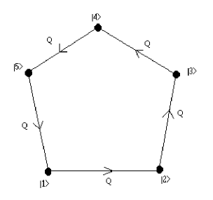
Figure 1: The vertices of this polygon represents the $k$ Laughlin wavefunctions (here we have taken a pentagon with $k=5$ vertices). The dots are associated with the $k$ characters of ${\hbox{\mybb Z}}_{k}$ and are rotated under ${\bf Q}$ automorphisms as shown on the figure. The factorisation of the ${\hbox{\mybb Z}}_{k}$ invariance implies the shrinking of the $k$ vertices down to $j=k$ and as a consequence one recovers the usual degenerate expression obtained in [3].

2.2 Non–commutative matrix model

In this section we want to extend the previous results, especially those in connection with discrete symmetries and NC geometry for the matrix model formulation [1, 2] of the Laughlin states $\nu={1\over k}$ . In this formulation, the $N$ classical particles are roughly speaking described by the $Z_{\alpha\alpha}$ diagonal entries of a $N\times N$ matrix $Z$ while their “mutual interactions” are carried by the non-diagonal terms $Z_{\alpha\beta},\alpha\neq\beta$. The corresponding creation and annihilation operators $a_{\alpha\beta}^{\pm}$ of the quantum system are valued in ${\rm{\bf Adj}}(U\left(N\right))$, contrary to the previous study where they were in the ${\bf N}$ and ${\bf{\bar{N}}}$ representations. We will give here below a correspondence rule allowing one to obtain the spectrum of the matrix model just from the results of the analysis of subsection (2.1). This derivation allows us to discover another remarkable property of the Polychronachos field operator and shows that this field operator is just the leading one of a more general situation to be considered in section 4.

For a system with a finite number $N$ of electrons, the action of the matrix model reads, in terms of the $Z$ and ${\bar{Z}}$ dynamical variables, as

$$S={\frac{k}{4\theta}}\int dt\;{\rm{Tr}}\left(i{\bar{Z}}DZ-\omega Z{\bar{Z}}\right)+\frac{i}{2}\int dt\;\Psi^{\dagger}D\Psi+\frac{k}{2}\int dt\;{\rm{Tr}}A+hc.$$ (89)

The matrix variables involved in this Lagrange description are: (i) A complex $(0+1)D$ field $Z(t)$ consisting of two hermitian $N\times N$ matrix fields: $X_{ij}^{1}$ and $X_{ij}^{2}$ transforming in the $U(N)$ adjoint representation ${\bf N}\otimes{\bf{\bar{N}}}$. (ii) The Polychronakos field $\Psi$ in the $U(N)$ fundamental representation ${\bf N}$ and (iii) the Lagrange matrix field $A_{0}$ transforming in ${\bf N}\otimes{\bf{\bar{N}}}$ and carrying the constraint of the system. In addition to the usual $\left(Z-Z\right)$, $\left(Z-A-Z\right)$, and $\left(\Psi-A\right)$ couplings, there is moreover a harmonic oscillator potential term $\left(\omega Z{\bar{Z}}\right)$ serving to glue together the electrons on a disc forming then a droplet system of radius $R\sim\sqrt{\frac{2\left(k+1\right)N}{B}}$ and an area [5]

$$2\pi R^{2}={2\pi\over N}{\rm{Tr}}Z{\bar{Z}}.$$ (90)

The above action has a one-dimensional $U(N)=U(1)\times SU(N)$ gauge invariance which can be used to fix the extra non-physical degrees of freedom involved in the above action. The presence of the term $\frac{k}{2}\int dt\;{\rm{Tr}}A$ shows that (89) is actually a constrained system. This constraint equation, which reads as

$$[Z,{\bar{Z}}]_{mn}+\frac{\theta}{2k}\Psi_{m}\Psi_{n}^{+}=\frac{1}{2}\theta\delta_{mn}\;$$ (91)

requires that the $\left(N^{2}-1\right)$ charge operators of the $SU\left(N\right)\subset U(N)$ gauge invariance are constrained to zero, while the $U(1)$ charge is fixed to the value $Nk$ as shown in (8).

Introducing the $N^{2}$ creation and $N^{2}$ annihilation operators

$$\begin{array}[]{l}b_{\alpha\beta}^{+}\equiv\sqrt{\frac{k}{2\theta}}(X_{\alpha\beta}+iY_{\alpha\beta})=\sqrt{\frac{k}{2\theta}}Z_{\alpha\beta},\ \ (N\;{\it operators}\;\Psi_{\alpha}^{+})\\ b_{\alpha\beta}^{-}\equiv\sqrt{\frac{k}{2\theta}}(X_{\alpha\beta}-iY_{\alpha\beta})=\sqrt{\frac{k}{2\theta}}{\bar{Z}}_{\alpha\beta},\ \ (N\;{\it{operators}}\;\Psi_{\alpha}^{-})\end{array}$$ (92)

one can derive the quantum spectrum of the action (89) by following the same lines of argument we have made earlier. The same results may be also derived directly by using the following correspondence rule: (i) Insert NC geometry effects by introducing the internal structure which allows the replacement of $b_{\alpha\beta}^{\pm}$ by the more general ones $\left({\bf b}^{\pm}\right)_{\alpha i_{\alpha}}^{\bar{\alpha}i_{\bar{\alpha}}}$ (ii) Associate with the operators $a_{\alpha i_{\alpha}}^{+}$ of subsection (2.1), transforming as $\left({\bf N},{\bf k}\right)$ under $SU(N)\otimes SU(k)$, the two following operators $\left({\bf b}^{+}\right)_{\alpha i_{\alpha}}^{\bar{\alpha}i_{\bar{\alpha}}}$ and ${\bf\psi}_{\alpha i_{\alpha}}^{+}$ transforming respectively as $\Big{(}{\bf adj}(U(N)),{\bf adj}(U(k))\Big{)}$ and $\left({\bf N},{\bf k}\right).$ Here the ${\bf\psi}_{\alpha i_{\alpha}}^{+}$’s are the creation operators associated with the $\Psi$ field and the annihilation operators are in the complex conjugate representations. The novelty here is that the creation and annihilation associated to the $Z$ and $\bar{Z}$ matrix variables carry $\left(2+2\right)$ indices. The $\Psi$ representation turns out to be the field one needs to reduce by contraction these indices down to a $\left({\bf N},{\bf k}\right)$ representation as shown on the following relation

$$a_{\alpha i_{\alpha}}^{+}\ \ \longrightarrow\ \ \ {\bf a}_{\alpha i_{\alpha}}^{+}=\left({\bf\psi}^{+}\cdot{\bf b}^{+}\right)_{\alpha i_{\alpha}}$$ (93)

where

$$\left({\bf\psi}^{+}\cdot{\bf b}^{+}\right)_{\alpha i_{\alpha}}=\sum_{\beta=\bar{\beta}=1}^{N}\sum_{j_{\beta}=1}^{k}{\bf\psi}_{\beta j_{\beta}}^{+}{\bf b}_{\alpha i_{\alpha}}^{+\bar{\beta}j_{\bar{\beta}}}.$$ (94)

This ${\bf a}_{\alpha i_{\alpha}}^{+}$ operator carries one energy excitation $\left({\bf b}^{+}\right)$ and one $U\left(1\right)$ charge since

$$\left[J_{0},{\bf a}_{\alpha i_{\alpha}}^{+}\right]=+{\bf a}_{\alpha i_{\alpha}}^{+}$$ (95)

where $J_{0}$ is the operator counting the number ${\bf\psi}^{+}$’s as shown in (8). A similar result is also valid for the $A_{\alpha j}^{\pm}\ \pi_{j}$ composite operators (76,78). In this case, the correspondence rule is

$$A_{\alpha}^{+}=\sum_{l=1}^{k}A_{\alpha l}^{+}\pi_{l}\ \ \ \rightarrow\ \ {\bf A}_{\alpha}^{+}=\sum_{l=1}^{k}{\bf A}_{\alpha l}^{+}\pi_{l}$$ (96)

and

$$\sum_{l=1}^{k}{\bf A}_{\alpha l}^{+}\pi_{l}=\sum_{l=1}^{k}<l|\varepsilon^{i_{1}\dots i_{k}}{\bf a}_{\alpha i_{1}}^{\pm}\dots{\bf a}_{\alpha i_{k}}^{\pm}|l>\pi_{l}$$ (97)

where the ${\bf a}_{\alpha i_{j}}^{\pm}$’s, are given in (93) and the $\pi_{j}$’s are the projectors on the states $|j\rangle$ introduced earlier. The ${\bf A}_{\alpha l}^{+}$ operators carry $k$ energy excitation units and $k$ charges of $U\left(1\right)$; i.e.

$$\left[J_{0},{\bf A}_{\alpha l}^{+}\right]=+k{\bf A}_{\alpha l}^{+}.$$ (98)

Note in passing that (93,96) are not the unique way to get condensate representation from the $\left({\bf b}^{+}\right)_{\alpha i_{\alpha}}^{\bar{\alpha}i_{\bar{\alpha}}}$’s and the ${\bf\psi}_{\alpha i_{\alpha}}^{+}$’s. One may also define other classes of $SU\left(k\right)$ invariants in an analogous way to what we have done for (93). For instance, one can define the two following condensates

$$\begin{array}[]{l}\Psi_{\alpha}^{\pm}=\sum_{l=1}^{k}<l|\Psi_{\alpha}^{\pm}|l>\pi_{l}\\ <l|\Psi_{\alpha}^{\pm}|l>=\varepsilon^{i_{1}\dots i_{l}}{\bf\psi}_{\alpha i_{1}}^{\pm}\dots{\bf\psi}_{\alpha i_{l}}^{\pm}\end{array}$$ (99)

and

$$\begin{array}[]{l}\left({\bf B}^{\pm}\right)_{\alpha}^{\bar{\alpha}}=\sum_{l_{1},l_{2}=1}^{k}<l_{1},l_{2}|\left({\bf B}^{\pm}\right)_{\alpha}^{\bar{\alpha}}|l_{1},l_{2}>\pi_{l_{1}l_{2}}\\ <l_{1},l_{2}|\left({\bf B}^{\pm}\right)_{\alpha}^{\bar{\alpha}}|l_{1},l_{2}>=\varepsilon^{i_{1}\dots i_{l_{1}}}\ \varepsilon_{j_{1}\dots j_{l_{2}}}\left({\bf b}^{\pm}\right)_{\alpha i_{1}}^{\bar{\alpha}j_{1}}\dots\left({\bf b}^{\pm}\right)_{\alpha i_{l_{1}}}^{\bar{\alpha}j_{l_{2}}}\end{array}$$ (100)

where $\pi_{ij}=\pi_{i}\otimes\pi_{j}$. The $\Psi_{\alpha}^{+}$ operators carry $k$ charges of $U\left(1\right)$ since

$$\left[J_{0},\Psi_{\alpha}^{+}\right]=+k\Psi_{\alpha}^{+}\;$$ (101)

while $\left({\bf B}^{\pm}\right)_{\alpha}^{\bar{\alpha}}$ carry $k$ units of the energy excitations. In terms of these operators and following the same philosophy as before, we can build an object

$${\bf E}_{\alpha}^{+}=\left(\Psi^{+}\cdot{\bf B}^{+}\right)_{\alpha}$$ (102)

where

$$\left(\Psi^{+}\cdot{\bf B}^{+}\right)_{\alpha}=\sum_{\beta=1}^{N}\Psi_{\beta}^{+}\left({\bf B}^{+}\right)_{\alpha}^{\bar{\beta}}\;$$ (103)

carrying $k$ charges of $U\left(1\right)$ and $k$ energy excitation units, exactly as for the composite ${\bf A}_{\alpha l}^{+}$ of (96). In fact due to the factorisation (48), the ${\bf A}_{\alpha}^{+}$ and ${\bf E}_{\alpha}^{+}$ are proportional and then we will use the ${\bf A}_{\alpha}^{+}$ objects.

One can also deduce the Hamiltonian ${\cal H}$ associated with the matrix model by using (60). It reads in terms of the $\left({\bf a}^{\pm}\right)_{\alpha i_{\alpha}}^{\beta j_{\beta}}$’s as

$${\cal H}={\omega\over 2}\Big{(}2{\cal N}_{b}+N^{2}\Big{)}$$ (104)

where ${\cal N}_{b}$ is the number operator counting $\left({\bf b}^{\pm}\right)_{\alpha}^{\bar{\alpha}}.\left({\bf Q}^{\pm 1}\otimes{\bf Q}^{\pm 1}\right)$. It is proportional to the sum over the $N^{2}$ number operator $\left({\bf b}^{+}\right)_{\alpha}^{\bar{\alpha}}\left({\bf b}^{-}\right)_{\alpha}^{\bar{\alpha}}$ times the $\left({\bf I}_{k}\otimes{\bf I}_{k}\right)$ identity operator. The wavefunctions can also be worked out immediately from (82); all one has to do is to replace the $A_{\alpha}^{+}$ operators of (82) by the expressions (93,96).

The above relations may also be derived by following the standard approach. The commutation relations for the matrix model are given by

$$\begin{array}[]{l}\left[\left({\bf b}^{-}\right)_{\alpha i_{\alpha}}^{\bar{\alpha}i_{\bar{\alpha}}},\left({\bf b}^{+}\right)_{\beta j_{\beta}}^{\bar{\beta}j_{\bar{\beta}}}\right]=\delta_{\alpha\beta}\delta^{\bar{\alpha}\bar{\beta}}\delta_{i_{\alpha}j_{\beta}}\delta^{{{i}}_{\bar{\alpha}}{{j}}_{\bar{\beta}}}\\ \left[{\bf\psi}_{\alpha i_{\alpha}}^{-},{\bf\psi}_{\beta j_{\beta}}^{+}\right]=\delta_{\alpha\beta}\delta_{i_{\alpha}j_{\beta}}\\ \left[\left({\bf b}^{\pm}\right)_{\alpha i_{\alpha}}^{\bar{\alpha}i_{\bar{\alpha}}},\left({\bf b}^{\pm}\right)_{\beta i_{\beta}}^{\bar{\beta}i_{\bar{\beta}}}\right]=0\\ \left[\left({\bf b}^{\pm}\right)_{\alpha i_{\alpha}}^{\bar{\alpha}i_{\bar{\alpha}}},{\bf\psi}_{\beta j_{\beta}}^{\pm}\right]=0\\ \left[{\bf\psi}_{\alpha i_{\alpha}}^{\pm},{\bf\psi}_{\beta j_{\beta}}^{\pm}\right]=0.\end{array}$$ (105)

Since $\left({\bf b}^{\pm}\right)_{\alpha i_{\alpha}}^{\bar{\alpha}i_{\bar{\alpha}}}$ and ${\bf\psi}_{\alpha i_{\alpha}}^{\pm}$ may also be expressed in a condensed form by using the realization (48) as follows

$$\sum_{i_{\alpha},i_{\bar{\alpha}}=1}^{N}\left({\bf b}^{\pm}\right)_{\alpha i_{\alpha}}^{\bar{\alpha}i_{\bar{\alpha}}}=\left({\bf b}^{\pm}\right)_{\alpha}^{\overline{\alpha}}.\left({\bf Q}^{\pm 1}\otimes{\bf Q}^{\pm 1}\right)\;$$ (106)

namely

$$\sum_{i_{\alpha},i_{\bar{\alpha}}=1}^{N}\left({\bf b}^{\pm}\right)_{\alpha i_{\alpha}}^{\bar{\alpha}i_{\bar{\alpha}}}=\left({\bf b}^{\pm}\right)_{\alpha}^{\bar{\alpha}}\sum_{i_{\alpha},i_{\bar{\alpha}}=1}^{N}{\bf f}_{i_{\alpha}}\ {\bf f}_{i_{\bar{\alpha}}}$$ (107)

and similarly

$$\sum_{i_{\alpha}=1}^{N}{\bf\psi}_{\alpha i_{\alpha}}^{\pm}={\bf\psi}_{\alpha}^{\pm}.{\bf Q}^{\pm 1}\;$$ (108)

the above commutation relations can be rewritten as

$$\begin{array}[]{l}\left[\left({\bf b}^{-}\right)_{\alpha}^{\bar{\alpha}},\left({\bf b}^{+}\right)_{\beta}^{\bar{\beta}}\right]=\delta_{\alpha\beta}\delta^{\bar{\alpha}\bar{\beta}}\\ \left[{\bf\psi}_{\alpha}^{-},{\bf\psi}_{\beta}^{+}\right]=\delta_{\alpha\beta}\\ \left[\left({\bf b}^{\pm}\right)_{\alpha}^{\bar{\alpha}},\left({\bf b}^{\pm}\right)_{\beta}^{\bar{\beta}}\right]=0\\ \left[\left({\bf b}^{\pm}\right)_{\alpha}^{\bar{\alpha}},{\bf\psi}_{\beta}^{\pm}\right]=0\\ \left[{\bf\psi}_{\alpha}^{\pm},{\bf\psi}_{\beta}^{\pm}\right]=0.\end{array}$$ (109)

Here also NC geometry lifts the degeneracy of the vacuum configurations with minimal energy $E_{v}={N\over 2}\Big{(}kN+k+1\Big{)}$ and $Nk$ charges of $U\left(1\right)$. The vacuum wavefunction of the FQH states at $\nu=\frac{1}{k}$ is in the centre of the ${\cal D}\left({\hbox{\mybb Z}}_{k}\right)$ representation and reads as

$$|\Phi_{v}^{\nu=1/k}\rangle={\cal N}\varepsilon^{\alpha_{1}\dots\alpha_{N}}({\bf A}{{}_{\alpha_{1}}^{+}})\Big{(}{\bf A}_{\alpha_{2}}^{+}\Big{)}^{2}\dots\Big{(}{\bf A}_{\alpha_{N}}^{+}\Big{)}^{N}\ {\bf I}\;|v\rangle$$ (110)

where ${\bf I}$ is the identity operator of ${\cal D}\left({\hbox{\mybb Z}}_{k}\right)$ and $|v\rangle$ the vacuum vector and the ${\bf A}{{}_{\alpha j}^{+}}$’s are as in (96). Viewed from the base of fibration ${\hbox{\mybb R}}_{\theta}^{2}\times{\cal D}\left({\hbox{\mybb Z}}_{k}\right)$, this relation reduces to the Hellermann and Van Raamsdonk (HR) wavefunction $|\Phi_{HR}>$ obtained in [3] and which reads, in terms of our notational convention, as

$$|\Phi_{HR}^{\nu=\frac{1}{k}}>={\cal N}\varepsilon^{\alpha_{1}\dots\alpha_{N}}\Big{(}\Psi^{+}.{C_{\alpha_{1}}^{+}}\Big{)}\Big{(}\Psi^{+}.\Big{(}C_{\alpha_{2}}^{+}\Big{)}^{2}\Big{)}\dots\Big{(}\Psi^{+}.\Big{(}C_{\alpha_{N}}^{+}\Big{)}^{N}\Big{)}|0\rangle.$$ (111)

Recall that in this representation, the vacuum $|0>$ ignores all aspects of the ${\hbox{\mybb Z}}_{k}$ symmetry of the Laughlin wavefunctions.

3 $\nu_{k_{1}k_{2}}$ Fractional quantum Hall states

Although the $\nu=\frac{2}{5}$ FQH state is not of the Laughlin type, it shares, however, some basic features of Laughlin fluids. The point is that from the standard definition of the filling factor $\nu=\frac{N}{N_{\phi}}$, the state $\nu=\frac{2}{5}$ can naively be thought of as corresponding to $\nu=\frac{N}{N_{\phi}}$ where the number $N_{\phi}$ of flux quanta is given by a fractional amount of the electron number; that is

$$N_{\phi}=(3-{\frac{1}{2}})N.$$ (112)

In fact this way of viewing things reflects just the original idea of the hierarchical construction of FQH states of general filling factor $\frac{p}{q}$, considered years ago by many FQH authors. In Haldane’s hierarchy [22] construction, for instance, the $K_{IJ}$ matrix of (15) is taken as

$$K_{IJ}=\left(\begin{array}[]{cccccc}p_{1}&-1&&&&\\ -1&p_{2}&-1&&&\\ &-1&.&.&&\\ &&.&.&.&\\ &&&.&.&-1\\ &&&&-1&p_{n}\end{array}\right)$$

with $p_{1}$ an odd integer and the others $p_{i}$’s even. The filling factor is given by the continuous fraction

$$\nu_{p_{1}...p_{n}}=\frac{1}{p_{1}-\frac{1}{p_{2-...}}}.$$ (113)

For the level two of the hierarchy $\left(n=2\right)$, the elements of the series

$$\nu_{p_{1}p_{2}}=\frac{p_{2}}{p_{1}p_{2}-1}$$ (114)

correspond to taking $N_{\phi}$ as given by a specific rational factor of the electron number; i.e.

$$N_{\phi}=(p_{1}-\frac{1}{p_{2}})N.$$ (115)

Upon setting

$$\begin{array}[]{l}k_{1}=p_{1}\\ k_{2}=k_{1}(k_{1}p_{2}-1)\end{array}$$ (116)

the rational factor $\frac{p_{1}p_{2}-1}{p_{2}}$ can be brought into the following suggestive form $\frac{k_{1}k_{2}}{k_{1}+k_{2}}$, and so the filling factor $\nu_{p_{1}p_{2}}\equiv\nu_{k_{1}k_{2}}$ splits as

$$\nu_{k_{1}k_{2}}=\frac{1}{k_{1}}+\frac{1}{k_{2}},\ \ \ \ \ k_{2}>k_{1}.$$ (117)

Therefore FQH states with $\nu_{k_{1}k_{2}}$ may, under some conditions, be thought of as consisting of two coupled Laughlin states of filling factors $\nu_{k_{1}}=\frac{1}{k_{1}}$ and $\nu_{k_{2}}=\frac{1}{k_{2}}$ respectively. The choice of $p_{1}$ an odd integer and $p_{2}$ even ensures automatically that both $k_{1}$ and $k_{2}$ are odd integers, and so both of the $\nu_{k_{i}}=\frac{1}{k_{i}}$ $(i=1,2)$ FQH branches describe fermions. This feature, which is valid for any level $n$ of the Haldane hierarchy, reads, for the special $\nu=\frac{2}{5}$ example we will be considering to illustrate our results, as

$$\nu=\frac{2}{5}\equiv\frac{1}{3}+\frac{1}{15}.$$ (118)

To study vacuum configurations of such FQH states, it is interesting to fix some terminology and specify the hypothesis we will be using. As far as terminology and notational convention are concerned, let $N_{1}$ (resp. $N_{\phi_{1}}$) be the number of electrons (resp. quantum flux) in the $\nu_{k_{1}}=\frac{1}{k_{1}}$ FQH fundamental state and $N_{2}$ (resp. $N_{\phi_{2}}$) be the number of electrons (resp. quantum flux) in $\nu_{2}=\frac{1}{k_{2}}$. From the relation $\nu_{k_{i}}=\frac{1}{k_{i}}$, we have the identities $N_{\phi_{i}}=k_{i}N_{i}$. Let also $B\equiv B_{1}$ be the external magnetic field viewed by the $N_{1}$ electrons of the $\nu_{k_{1}}$ FQH fundamental state and $B^{\ast}\equiv B_{2}$ be the effective magnetic field felt by the $N_{2}$ electrons of the $\nu_{k_{2}}$ hierarchical state. The relation between the $B$ and $B^{\ast}$ fields is

$$\frac{B_{2}}{B_{1}}=\frac{k_{2}}{k_{1}}\equiv\left(k_{1}p_{2}-1\right).$$ (119)

For the $\nu=\frac{2}{5}$ state, we have the relation $B_{2}=5B_{1}$. A way to derive this result is to use the following semi-classical analysis. First denote by $\left\{Z_{1,\alpha},{\bar{Z}}_{1,\alpha};1\leq\alpha\leq N_{1}\right\}$ the quantum coordinate operators associated with the $\nu_{k_{1}}=\frac{1}{k_{1}}$ state and by $\left\{Z_{2,a},{\bar{Z}}_{2,a};1\leq a\leq N_{2}\right\}$ those associated with the $\nu_{k_{2}}=\frac{1}{k_{2}}$ state. The dynamics of these two sets of matrix variables is given by actions of type (89). Then use the following quantum constraint equations by treating for the moment the two Laughlin states $\nu_{k_{1}}$ and $\nu_{k_{2}}$ as independent:

$$\begin{array}[]{l}\left[Z_{1,\alpha},{\bar{Z}}_{1,\beta}\right]=i\theta_{1}\delta_{\alpha\beta}\\ \left[Z_{2,a},{\bar{Z}}_{2,b}\right]=i\theta_{2}\delta_{ab}\end{array}$$ (120)

where, according to the result of Susskind, the $\theta_{j}$ parameters in the large $N$ limits are given by

$$\theta_{j}={\rm const}\;\frac{k_{j}}{B_{j}}.$$ (121)

Since $\theta_{j}$ is interpreted as the effective size occupied by an electron in the quantum space ${\hbox{\mybb R}}_{\theta}^{2}$, it follows from the indiscernability hypothesis that $\theta_{1}=\theta_{2}$ and consequently

$$\frac{k_{1}}{B_{1}}=\frac{k_{2}}{B_{2}}.$$ (122)

Setting $B_{i}=l_{i}^{-2}$ where $l_{1}$ and $l_{2}$ are the so-called magnetic lengths associated to $B_{1}$ and $B_{2}$ respectively, the previous relation then reads as

$$k_{i}l_{i}^{2}={\rm const}.$$ (123)

As we are dealing with $N=\left(N_{1}+N_{2}\right)$ electrons coming from two origins and since $k_{2}>k_{1}$, it is helpful to introduce the following useful terminology. Thus we will refer to the elementary flux $\phi_{1}$ occupying the area ${\cal A}_{1}\sim\frac{1}{B_{1}}=l_{1}^{2}$ in the $\nu_{k_{1}}$ state as quasi-electrons and to those elementary fluxes $\phi_{2}$, of size ${\cal A}_{2}\sim\frac{1}{B_{2}}=l_{2}^{2}$, in the $\nu_{k_{2}}$ state as quasi-muons. This terminology should not be confused with various ones used in condensed matter physics literature. In our case, all that this appellation means is that when $k_{1}$ quasi-electrons (resp. $k_{2}$ quasi-muons) condensate, they give rise to one real electron (resp. one muon by extension).

Using the results of section 2, one can first write down the fundamental wavefunctions $|\Phi_{1},v_{k_{1}}\rangle\otimes|\Phi_{2},v_{k_{2}}\rangle$ for the uncoupled system; that is for the situation where each of the filling factors $\nu_{k_{1}}$ and $\nu_{k_{2}}$ are treated separately. This is the case for instance of two FQH layers distant enough so that they cannot feel each other. However, this is not the case here. The system in the present study consists of one layer only and the $\nu_{k_{1}}$ and $\nu_{k_{2}}$ states should be coupled. If we denote by $a_{\alpha i_{\alpha}}^{+}$ the creation operators of quasi-electrons (resp. $d_{ai_{a}}^{+}$ the creation operators of quasi-muons) and by $A_{\alpha}^{+}$ the creation operators of one electron with energy $k_{1}$ in $\omega_{1}$ units and $k_{1}$ charges of $U\left(1\right)$ (76,78) (resp. $D_{a}^{+}$ the creation operator of muons with energy $k_{2}$ in $\omega_{2}$ units and $k_{2}$ charges of $U^{\prime}\left(1\right)$ (76,78)), then the wavefunction $|\Phi_{v_{12}}\rangle$ describing the vacuum configuration of $N=\left(N_{1}+N_{2}\right)$ particles is (with the hypothesis $N_{1}=rN_{2}$ , $r>1$, as is usually the case for the level two of the Haldane hierarchy)

$$|\Phi_{v_{12}}\rangle=\varepsilon^{I_{1}\dots I_{r}}[{\cal A}^{+}]_{I_{1}}[{{\cal A}^{+}(}D{{}^{+})^{1}]}_{I_{2}}\dots[{{\cal A}^{+}(}D{{}^{+})^{r-1}]}_{I_{r}}|0,(s_{1},s_{2})\rangle$$ (124)

where $I_{j}$ stands for a multi-index

$$I_{j}=(\beta_{jN_{2}},\beta_{jN_{2}+1},\dots,\beta_{jN_{2}+({N_{2}-1})})$$ (125)

indexing the $j$-th block; the tensor $\varepsilon^{I_{1}\dots I_{r}}$ is the usual $SU\left(N_{1}\right)$ invariant antisymmetric tensor expressed in terms of multi-indices; that is

$$\varepsilon^{I_{1}\dots I_{r}}=\varepsilon^{\beta_{1}\dots\beta_{N_{2}}\dots\beta_{rN_{2}}\ldots\beta_{(r+1)N_{2}-1}}$$ (126)

and where the $\left[{\cal A}^{+}{\left(D^{+}\right)^{j-1}}\right]_{I_{j}}$ building blocks are given by

$$\left[{\cal A}^{+}{\left(D^{+}\right)^{j-1}}\right]_{I_{j}}=\left(A^{+}{\left(D^{+}\right)^{j-1}}\right)_{\beta_{1}}\left(\left(A^{+}\right)^{2}\left(D^{+}\right)^{j-1}\right)_{\beta_{2}}\dots\left(\left(A^{+}\right)^{N_{2}}\left(D^{+}\right)^{j-1}\right)_{\beta_{N_{2}}}.$$ (127)

$|0,(s_{1},s_{2})\rangle$ is the vacuum state transforming as a $\left({\bf k}_{1}{\bf,k}_{2}\right)$ vector under ${\hbox{\mybb Z}}_{k_{1}}\otimes{\hbox{\mybb Z}}_{k_{2}}$ symmetry. The energy of the above vacuum configuration is directly obtained by computing the energy of the generic building blocs $\left[{\cal A}^{+}{\left(D^{+}\right)^{j-1}}\right]_{I_{j}}$. The latter have an energy contribution of the form $E_{A^{+}}+E_{D^{+}}$ associated with the $A^{+}$ and $D^{+}$ operators and respectively equal to

$$\begin{array}[]{l}E_{A^{+}}={1\over 2}k_{1}N_{2}\left(N_{2}+1\right)\\ E_{D^{+}}=(j-1)k_{2}N_{2}.\end{array}$$ (128)

Adding these two energies, one obtains

$$E_{A^{+}}+E_{D^{+}}={1\over 2}k_{1}N_{2}(N_{2}+1)+\left(j-1\right)k_{2}N_{2}.$$ (129)

Then summing over all allowed values of the index $j$; i.e. $1\leq j\leq r$, as required by the expression of the wavefunction $|\Phi_{v_{12}}\rangle$, by taking into account the relation $N_{1}=rN_{2}$, one gets

$$E_{A^{+}}+E_{D^{+}}=\frac{N_{1}}{2}\Big{[}k_{1}\left(N_{2}+1\right)+k_{2}\left(r-1\right)\Big{]}\;.$$ (130)

Taking into account the vacuum contribution of the oscillator which is equal to $\frac{N_{1}+N_{2}}{2}$, one ends up with the following relation for the vacuum energy of the interacting configuration

$$E_{v_{12}}^{\nu=1/k_{1}+1/k_{2}}=\frac{1}{2}\Big{\{}k_{1}N_{1}N_{2}+N_{1}\left[k_{2}\left(r-1\right)+k_{1}+1\right]+N_{2}\Big{\}}.$$ (131)

Note that for large values of $N_{1}$ and $N_{2}$, but $\frac{N_{1}}{N_{2}}=\frac{k_{2}}{k_{1}}$ finite, say

$$\begin{array}[]{l}N_{1}=rN_{2}\equiv rM\\ k_{2}=rk_{1}\end{array}$$ (132)

the vacuum energy of the configuration (124) behaves quadratically in $M$ with a coefficient $\frac{k_{2}}{2}$, namely

$$E_{v_{12}}^{\nu=\left(1/k_{1}+1/k_{2}\right)}\sim\frac{k_{2}}{2}M^{2}.$$ (133)

This energy relation is less than the total energy $\left(E_{v_{1}}^{\nu=1/k_{1}}+E_{v_{2}}^{\nu=1/k_{2}}\right)$ of the decoupled configuration $\left(|\Phi_{1},v_{k_{1}}\rangle\otimes|\Phi_{2},v_{k_{2}}\rangle\right)$ which also behaves quadratically in $M$ as shown here below; but with a coefficient $\frac{k_{2}\left(r+1\right)}{2}$ larger than that appearing in presence of interactions. Indeed, using (83,84), we obtain

$$E_{v_{1}}^{\nu=1/k_{1}}+E_{v_{2}}^{\nu=1/k_{2}}\sim\frac{k_{1}N_{1}^{2}}{2}+\frac{k_{2}N_{2}^{2}}{2}$$ (134)

leading to

$$E_{v_{1}}^{\nu=1/k_{1}}+E_{v_{2}}^{\nu=1/k_{2}}\sim\frac{k_{2}(r+1)}{2}\ M^{2}.$$ (135)

Therefore the difference between the energies $\left(E_{v_{1}}^{\nu=1/k_{1}}+E_{v_{2}}^{\nu=1/k_{2}}\right)$ and $E_{v_{12}}^{\nu=\left(1/k_{1}+1/k_{2}\right)}$ of the decoupled configuration and the interacting one is

$$\left(E_{v_{1}}^{\nu=1/k_{1}}+E_{v_{2}}^{\nu=1/k_{2}}\right)-E_{v_{12}}^{\nu=\left(1/k_{1}+1/k_{2}\right)}\sim\frac{k_{2}r}{2}\ M^{2}$$ (136)

showing that

$$\left(E_{v_{1}}^{\nu=1/k_{1}}+E_{v_{2}}^{\nu=1/k_{2}}\right)\sim\left(r+1\right)E_{v_{12}}^{\nu=\left(1/k_{1}+1/k_{2}\right)}.$$ (137)

For the example of the FQH state at filling factor $\nu=\frac{2}{5}$, the energy of the decoupled representation $\frac{2}{5}=\frac{1}{3}+\frac{1}{15}$ reads as

$$E_{v_{1}}^{\nu=1/3}+E_{v_{2}}^{\nu=1/15}\sim 45M^{2}$$ (138)

while that of the interacting one is

$$E_{v_{12}}^{\nu=\left(1/3+1/15\right)}\sim\frac{15}{2}M^{2}.$$ (139)

It is obvious to see that equations (138,139) verify the relation (137), such that

$$\left(E_{v_{1}}^{\nu=1/3}+E_{v_{2}}^{\nu=1/15}\right)\sim 6E_{v_{12}}^{\nu=\left(1/3+1/15\right)}.$$ (140)

In what follows, we propose a matrix model to describe such FQH states that are not of Laughlin type. We will focus our attention on the ${e}-{\mu}$ system we presented above although most of our results may be extended to more general FQH systems.

4 Matrix model for $({e}-{\mu})$ system

We start by presenting the variables of the matrix model for the case of a FQH droplet of $N=\left(N_{1}+N_{2}\right)$ electrons ($N_{1}$ electrons and $N_{2}$ muons) with filling factor $\nu_{k_{1}k_{2}}$. The integers $k_{1}$ and $k_{2}$ are some specific odd integers; they are essentially given by the family of integers, $k_{1}=p_{1}$ and $k_{2}=p_{1}(p_{1}p_{2}-1)$ with $p_{1}$ odd and $p_{2}$ even, appearing in the second level of the Haldane hierarchy. One of the key ideas of our description is to think about these states as consisting of two coupled branches of filling fractors $\nu_{k_{1}}=\frac{1}{k_{1}}$ and $\nu_{k_{2}}=\frac{1}{k_{2}}$. The second FQH state with $N_{2}$ muons is built on top of the $\nu_{k_{1}}$ state; that is it comes after the condensation of the $N_{1}$ electrons of the $\nu_{k_{1}}$ state, viewed, by the way, as the level one of the hierarchy. The matrix fields involved in our model are of three kinds: the first fields, which describe the set of $N_{1}$ electrons in the presence of the external magnetic field $B$, are associated with the $e$–sector, the second type of fields describe the $\mu$–sector and the third type of fields carry the $({e}-{\mu})$–couplings.

4.1 ${e}$–Sector

The matrix variables associated with the $e$–sector of the $({e}-{\mu})$ system are supposed to describe the $\nu_{k_{1}}=\frac{1}{k_{1}}$ branch of the fluid. They are given by the usual triplet $(Z_{1},\Psi_{1},A_{1})$ appearing in the Susskind-Polychronakos matrix model and have the following $U(N_{1})$ group structure

$$\begin{array}[]{l}Z_{1}=(Z_{1})_{\alpha}^{\bar{\alpha}}\sim{\bf N}_{1}\otimes{\bf{\bar{N}}}_{1}\\ {\bar{Z}}_{1}=({\bar{Z}}_{1})_{\bar{\alpha}}^{\alpha}\sim{{\bar{{\bf N}}}}_{1}\otimes{\bf N}_{1}\\ \Psi_{1}=(\Psi_{1})_{\alpha}\ \ \sim{\bf N}_{1}\\ {\bar{\Psi}}_{1}=({\bar{\Psi}_{1}})^{\bar{\alpha}}\ \ \sim{\bf{\bar{N}}}_{1}\\ A_{1}=(A_{1})_{\alpha}^{\bar{\alpha}}\sim{\bf N}_{1}\otimes{\bf{\bar{N}}}_{1}.\end{array}$$ (141)

The matrix model describing the dynamics of these fields is given by the following one-dimensional $U(N_{1})$ gauge invariant action

$${\cal S}_{1}={\frac{k_{1}}{4\theta_{1}}}\int dt\;{\rm{Tr}}\left(i{\bar{Z}_{1}}DZ_{1}-\omega_{1}{\bar{Z}_{1}}Z_{1}\right)+\frac{i}{2}\int dt\;{\bar{\Psi}}_{1}D\Psi_{1}+\frac{k_{1}}{2}\int dt\;{\rm{Tr}}A_{1}+hc$$ (142)

while the constraint equations, which are obtained as usual by computing the equation of motion of $A_{1}$, read as

$$[Z_{1},{\bar{Z}_{1}}]_{\alpha}^{\bar{\alpha}}+\frac{\theta_{1}}{2k_{1}}\Psi_{\alpha}{\bar{\Psi}}^{\bar{\alpha}}=\frac{1}{2}\theta_{1}\delta_{\alpha}^{\bar{\alpha}}.$$ (143)

Quantum mechanically, these constraint equations should be imposed on the Hilbert space ${\bf H}$ of the wavefunctions $|\Phi\rangle$ and so (143) should be thought of as

$$\begin{array}[]{l}J_{\alpha\bar{\alpha}}^{(1)}|\Phi\rangle=0\\ J_{0}^{(1)}|\Phi\rangle=\left(k_{1}N_{1}=\frac{N_{1}}{\nu_{1}}\right)|\Phi\rangle\end{array}$$ (144)

where $J_{0}^{(1)}$ and $J_{\alpha\bar{\alpha}}^{(1)}$ are the generators of the $U(N_{1})=U(1)\times SU(N_{1})$ gauge symmetry of the action ${\cal S}_{1}$. Later on we will give the field realization of these charge operators; but for the moment let us complete the presentation of the dynamical variables of the $(e-\mu)$ system.

4.2 ${\mu}$–Sector

The matrix field variables associated with the subsystem ${\bf\mu}$ containing $N_{2}$ electrons (muons) are quite similar to those appearing in the ${e}$–sector. These variables, which describe the $\nu_{k_{2}}$ branch of the $\nu_{k_{1}k_{2}}$ fluid, are given by the triplet $(Z_{2},\Psi_{2},A_{2})$ valued in $U(N_{2})$ group representations as shown below

$$\begin{array}[]{l}Z_{2}=(Z_{2})_{a}^{\bar{a}}\sim{\bf N}_{2}\otimes{\bf{\bar{N}}}_{2}\\ {\bar{Z}}_{2}=({\bar{Z}}_{2})_{\bar{a}}^{a}\sim{\bf\bar{N}}_{2}\otimes{\bf N}_{2}\\ \Psi_{2}=(\Psi_{2})_{a}\ \ \sim{\bf N}_{2}\\ {\bar{\Psi}}_{2}=({\bar{\Psi}_{2}})^{\bar{a}}\ \ \sim{\bf{\bar{N}}}_{2}\\ A_{2}=(A_{2})_{a}^{\bar{a}}\sim{\bf N}_{2}\otimes{\bf{\bar{N}}}_{2}.\end{array}$$ (145)

The action ${\cal S}_{2}$ of the matrix model for this sector reads as

$${\cal S}_{2}={\frac{k_{2}}{4\theta_{2}}}\int dt\;{\rm{Tr}}\left(i{\bar{Z}_{2}}DZ_{2}-\omega_{2}Z_{2}{\bar{Z}_{2}}\right)+\frac{i}{2}\int dt\;{\bar{\Psi}}_{2}D\Psi_{2}+\frac{k_{2}}{2}\int dt\;{\rm{Tr}}A_{2}+hc.$$ (146)

The constraint equations are naturally given by

$$[Z_{2},{\bar{Z}_{2}}]_{a}^{\bar{a}}+\frac{\theta_{2}}{2k_{2}}\Psi_{a}{\bar{\Psi}}^{\bar{a}}=\frac{1}{2}\theta_{2}\delta_{a}^{\bar{a}}.$$ (147)

At the quantum level, they should be thought of as

$$\begin{array}[]{l}J_{a\bar{a}}^{(2)}|\Phi\rangle=0\\ J_{0}^{(2)}|\Phi\rangle=\left(k_{2}N_{2}=\frac{N_{2}}{\nu_{2}}\right)|\Phi\rangle\end{array}$$ (148)

where now $J_{0}^{(2)}$ and $J_{a{\bar{a}}}^{(2)}$ are the generators of the $U(N_{2})=U(1)\times SU(N_{2})$ gauge symmetry of the action ${\cal S}_{2}$.

Note that as far as these two pieces of the total action ${\cal S=}\left({\cal S}_{1}+{\cal S}_{2}+{\cal S}_{int}\right)$ of the $(e-\mu)$ system are concerned, the full gauge symmetry is $U(N_{1})\times U(N_{2})$. The matrix model variables listed above transform under this invariance as

$$\begin{array}[]{l}Z_{i}\rightarrow U_{i}Z_{i}U_{i}^{\dagger}\\ \Psi_{i}\rightarrow U_{i}\Psi_{i}\\ A_{i}\rightarrow U_{i}(A_{i}-\partial_{t})U_{i}^{\dagger}\end{array}$$ (149)

where $i=1,2$ and the $U_{i}$ gauge transformations are given by

$$U_{i}=\exp\left(i\sum_{n=1}^{N_{i}}T_{n}\lambda_{i}^{n}(t)\right)$$ (150)

with $T_{n}$ being the group generators and $\lambda_{i}^{n}\left(t\right)$ the gauge parameters.

4.3 $(e-\mu)$–Couplings

Interactions between the ${e}-$sector and the ${\bf\mu}$ one consisting of the two branches of the $({e-\mu})$ fluid are introduced via three mechanisms: (i) Through the choice of the moduli parameters, (ii) the distribution of the fractional $D0$-branes on the droplet and (iii) via a gauge principle.

Concerning the first contribution to interactions, the point is that because of the presence of the ${e}$–sector, the particles of the ${\mu}$–sector (the muons) will feel not only the external magnetic field $B=B_{1}$ but also an induced term coming from the charged particles of the ${e}$–sector. As such electrons of the ${\bf\mu}$–sector view a total magnetic field

$$B^{\ast}=B_{2}=B_{1}+\Delta B.$$ (151)

From previous analysis, see (122,123), one learns that $B_{2}=\frac{k_{2}}{k_{1}}B_{1}$. The latter relation is based on the identity $\theta_{1}=\theta_{2}\equiv\theta$.

For the distribution of the $D0$-branes of the $\nu_{k_{1}k_{2}}$ FQH states, we suppose that the constraint equations $J_{0}^{(i)}|\Phi\rangle=N_{i}\nu_{k_{i}}^{-1}|\Phi\rangle$ established for the Laughlin states are general ones and so we demand that such a condition is also valid for FQH states that are not of the Laughlin type. Put differently, we will suppose that the total number of the fractional $D0$-branes in the vacuum configuration $|\Phi\rangle$ of the $\nu_{k_{1}k_{2}}$ FQH states is given by $J_{0}|\Phi\rangle=\frac{N}{\nu}|\Phi\rangle$; i.e

$$J_{0}|\Phi\rangle=\frac{k_{1}k_{2}}{k_{1}+k_{2}}N|\Phi\rangle$$ (152)

where the $J_{0}$ charge operator is the full charge operator to be given later.

The third contribution to interactions between the two branches of the $(e-\mu)$ fluid comes from the requirement that the ${e}$ and ${\bf\mu}$ couplings are $U(N_{1})\times U(N_{2})$ gauge invariant. From the $U(N_{1})\times U(N_{2})$ group representation analysis (141) and (145), one sees that the candidate fields to carry such interactions behave as

$$\begin{array}[]{l}\Psi_{\alpha a}\ \ \sim({\bf N}_{1},{\bf N}_{2})\\ {\bar{\Psi}}^{\bar{\alpha}\bar{a}}\ \ \sim({\bf{\bar{N}}}_{1},{\bf{\bar{N}}}_{2})\\ {\Psi}_{\alpha}^{\bar{a}}\ \ \sim({\bf N}_{1},{\bf{\bar{N}}}_{2})\\ {\bar{\Psi}}^{\bar{\alpha}}_{a}\ \ \sim({\bf{\bar{N}}}_{1},{\bf N}_{2}).\end{array}$$ (153)

Therefore, there are two kinds of rectangular complex matrices $\Psi_{\alpha a}$ and ${\Psi}_{\alpha}^{\bar{a}}$ together with their complex conjugates. They look like the Polychronakos field, but in fact they are more general objects with very remarkable features. To get more insight in the role played by these fields, let us focus our attention on one of these fields, say the $\Psi_{\alpha a}$ and its conjugate ${\bar{\Psi}}^{\bar{\alpha}\bar{a}}$. The results extend directly to the others.

4.4 Interactions

Now considering (141) and (145), and restricting to the $\Psi_{\alpha a}$ and ${\bar{\Psi}}^{\bar{\alpha}\bar{a}}$ fields, a possible $U(N_{1})\times U(N_{2})$ gauge invariant interacting action ${\cal S}_{int}$ one can write down, up to the fourth order in the fields, is

$$\begin{array}[]{l}{\cal S}_{int}=\frac{i}{2}\int dt\;\left({\bar{\Psi}}^{\bar{\alpha}\bar{a}}\partial_{t}\ \Psi_{\alpha a}+{\bar{\Psi}}^{\bar{\alpha}\bar{a}}{A_{1}}_{\alpha}^{\bar{\beta}}\Psi_{\beta a}+{\bar{\Psi}}^{\bar{\alpha}\bar{a}}{A_{2}}_{a}^{\bar{b}}\Psi_{\alpha b}+hc\right)\\ \qquad\;\;+\frac{i}{2}\int dt\left(g_{1}{\bar{\Psi}}^{\bar{\alpha}\bar{a}}{Z_{1}}_{\alpha}^{\bar{\beta}}\Psi_{\beta a}+g_{2}{\bar{\Psi}}^{\bar{\alpha}\bar{a}}Z_{2a}^{\bar{b}}\Psi_{\alpha b}+hc\right)\\ \qquad\;\;+\frac{i}{2}\int dt\;\left(g_{3}{\bar{\Psi}}^{\bar{\alpha}\bar{a}}{\Psi_{1}}_{\alpha}{\bar{\Psi}_{1}}^{\bar{\beta}}\Psi_{\beta a}+g_{4}{\bar{\Psi}}^{\bar{\alpha}\bar{a}}\Psi_{2a}{\bar{\Psi}_{2}}^{\bar{b}}\Psi_{\alpha b}+g_{5}{\bar{\Psi}}^{\bar{\alpha}\bar{a}}{Z_{1}}_{\alpha}^{\bar{\beta}}Z_{2a}^{\bar{b}}\Psi_{\beta b}+hc\right).\end{array}$$ (154)

In this relation the $SU\left(N_{1}\right)$ indices $\alpha$, $\bar{\alpha}$ $\left({\rm{resp.}}\;SU\left(N_{2}\right){\rm{indices}}\;a,\bar{a}\right)$ are contracted and the summation over the range $1\leq\alpha=\bar{\alpha}\leq N_{1}$ $\left({\rm{resp}}.\;1\leq a=\bar{a}\leq N_{2}\right)$ is understood. The five $g_{i}$ parameters are special coupling constants involving a product of the $\Psi_{\alpha a}$ field and its conjugate; there exist other coupling parameters which are not important for the forthcoming analysis and which we have set to zero for simplicity. Note in passing that due to the $\Psi_{\alpha a}$ field, the term $g_{5}{\bar{\Psi}}^{\bar{\alpha}\bar{a}}{Z_{1}}_{\alpha}^{\bar{\beta}}Z_{2a}^{\bar{b}}\Psi_{\beta b}$ involves couplings of the ${Z_{1}}$ and ${Z_{2}}$ matrix variables already at the fourth order in the fields, while one needs to go to the sixth power if one is using only the Polychronakos type fields as shown in the following interacting term, ${\bar{\Psi}}_{1}^{\bar{\alpha}}{\bar{\Psi}}_{2}^{\bar{a}}\ {Z_{1}}_{\alpha}^{\bar{\beta}}Z_{2a}^{\bar{b}}\Psi_{1\beta}\Psi_{2b}$.

The constraint equations one gets from the full action ${\cal S}$ of the $({e}-{\mu})$ system contain extra contributions coming from the interacting part (154). The new quantum constraint equations read therefore as

$$\begin{array}[]{l}J_{\alpha\bar{\alpha}}^{(1)}|\Phi\rangle=0\\ J_{0}^{(1)}|\Phi\rangle=k_{1}N_{1}|\Phi\rangle\\ J_{a\bar{a}}^{(2)}|\Phi\rangle=0\\ J_{0}^{(2)}|\Phi\rangle=k_{2}N_{2}|\Phi\rangle\end{array}$$ (155)

where now the $U(N_{1})\times U(N_{2})$ currents have a $\Psi_{\alpha a}$ and ${\bar{\Psi}}_{\bar{\alpha}{\bar{a}}}$ dependence as shown below

$$\begin{array}[]{l}J_{\alpha\bar{\alpha}}^{(1)}=[Z_{1},{\bar{Z}_{1}}]_{\alpha\bar{\alpha}}+\frac{\theta}{2k_{1}}\left(\Psi_{1\alpha}{\bar{\Psi}}_{1{\bar{\alpha}}}+\sum_{a=1}^{N_{2}}\Psi_{\alpha a}{\bar{\Psi}}_{{\bar{\alpha}}{\bar{a}}}-J_{0}^{(1)}\delta_{\alpha\bar{\alpha}}\right)\\ J_{0}^{(1)}=\sum_{\alpha=1}^{N_{1}}\left({\bar{\Psi}}_{1\bar{\alpha}}\Psi_{1\alpha}+\sum_{a=1}^{N_{2}}{\bar{\Psi}}_{{\bar{\alpha}}{\bar{a}}}\Psi_{\alpha a}\right)\end{array}$$ (156)

and similar relations for the $\mu$–sector

$$\begin{array}[]{l}J_{a\bar{a}}^{(2)}=[Z_{2},{\bar{Z}_{2}}]_{a\bar{a}}+\frac{\theta}{2k_{2}}\left(\Psi_{2a}{\bar{\Psi}}_{2\bar{a}}+\sum_{\alpha=1}^{N_{1}}\Psi_{\alpha a}{\bar{\Psi}}_{\bar{\alpha}{\bar{a}}}-J_{0}^{(2)}\delta_{a\bar{a}}\right)\\ J_{0}^{(2)}=\sum_{a=1}^{N_{2}}\left({\bar{\Psi}}_{2\bar{a}}\Psi_{2a}+\sum_{\alpha=1}^{N_{1}}{\bar{\Psi}}_{\bar{\alpha}{\bar{a}}}\Psi_{\alpha a}\right).\end{array}$$ (157)

It is interesting to note here that as far as consistency of the matrix model is concerned, one does not need to introduce all the different kinds of the $\Psi$’s we have considered above. It is possible to accomplish our objective with the $\Psi_{\alpha a}$ field in the bi-fundamental of the $U(N_{1})\times U(N_{2})$ gauge group.

4.5 $(e-\mu)$–Matrix model

In this special matrix model, the $\Psi_{1\alpha}$ and $\Psi_{2a}$ Polychronakos fields and the ${\Psi}_{\alpha}^{\bar{a}}$ field are ignored and  so the effective variables of the $(e-\mu)$ system are reduced to $\left\{Z_{1},Z_{2},A_{1},A_{2},\Psi_{\alpha a}\right\}$, while the total action ${\cal S}$, obtained from (154) by setting also $g_{1}=g_{2}=0$, reads as

$$\begin{array}[]{l}{\cal S}=\int dt\;\sum_{i=1}^{2}\Big{[}{\frac{k_{i}}{4\theta}}{\rm{Tr}}\left(i{\bar{Z}_{i}}DZ_{i}-\omega{\bar{Z}_{i}}Z_{i}+2\theta A_{i}\right)\Big{]}+hc\\ \;\;\;+\int dt\;\left[\frac{i}{2}{\bar{\Psi}}^{\bar{\alpha}\bar{a}}\left(\partial_{t}+{A_{1}}_{\alpha}^{\bar{\beta}}\delta_{a}^{\bar{b}}+{A_{2}}_{a}^{\bar{b}}\delta_{\alpha}^{\bar{\beta}}\right)\Psi_{\bar{\beta}\bar{b}}+\lambda{\bar{\Psi}}^{\bar{\alpha}\bar{a}}{Z_{1}}_{\alpha}^{\bar{\beta}}Z_{2a}^{\bar{b}}\Psi_{\beta b}\right]+hc\end{array}$$ (158)

where we have set $\omega_{1}=\omega_{2}=\omega$. The above realization of the $J_{\alpha\bar{\alpha}}^{(1)}$ and $J_{a\bar{a}}^{(2)}$ currents (156,157) simplifies to

$$\begin{array}[]{l}J_{\alpha\bar{\alpha}}^{(1)}=[Z_{1},{\bar{Z}_{1}}]_{\alpha\bar{\alpha}}+\frac{\theta}{2k_{1}}\left(\sum_{a=1}^{N_{2}}\Psi_{\alpha a}{\bar{\Psi}}_{\bar{\alpha}{\bar{a}}}-J_{0}^{(1)}\delta_{\alpha\bar{\alpha}}\right)\\ J_{a\bar{a}}^{(2)}=[Z_{2},{\bar{Z}_{2}}]_{a\bar{a}}+\frac{\theta}{2k_{2}}\left(\sum_{\alpha=1}^{N_{1}}\Psi_{\alpha a}{\bar{\Psi}}_{\bar{\alpha}{\bar{a}}}-J_{0}^{(2)}\delta_{a\bar{a}}\right)\end{array}$$ (159)

while the two $U(1)$ charge operators $J_{0}^{(1)}$ and $J_{0}^{(2)}$ reduce to

$$\begin{array}[]{l}J_{0}^{(1)}=\sum_{\alpha=1}^{N_{1}}\left(\sum_{a=1}^{N_{2}}\ \ {\bar{\Psi}}_{\bar{\alpha}{\bar{a}}}\Psi_{\alpha a}\right)\\ J_{0}^{(2)}=\sum_{a=1}^{N_{2}}\left(\sum_{\alpha=1}^{N_{1}}\ \ {\bar{\Psi}}_{\bar{\alpha}{\bar{a}}}\Psi_{\alpha a}\right).\end{array}$$ (160)

Comparing these two relations, one discovers, upon interverting the sums $\sum_{\alpha=1}^{N_{1}}$ and $\sum_{a=1}^{N_{2}}$, that the two $U(1)$ charge currents are equal, i.e $J_{0}^{(1)}=J_{0}^{(2)}$. So the number $k_{1}N_{1}$ of quasi-electrons and the number $k_{2}N_{2}$ of quasi-muons in the vacuum configuration of the $(e-\mu)$ droplet should be equal; that is we should have the equality

$$k_{1}N_{1}=k_{2}N_{2}.$$ (161)

This constraint equation is not a strange relation; it is in fact expected from group theoretical analysis of the vacuum wavefunction and a result of subsection (2.2). Indeed, due to non-commutative geometry, the $SU\left(k_{1}\right)$ and $SU\left(k_{2}\right)$ singularities of the Laughlin wavefunctions of the ${e}$ and $\mu$ sectors are removed and therefore the classical $\Psi$ field in the bi-fundamental (153) should be replaced, at the quantum level, by the $\Psi_{\alpha i_{\alpha},aj_{a}}^{\pm}$ operators transforming in the $\left({\bf N}_{1}{\bf,k}_{1}\right)\otimes\left({\bf N}_{2}{\bf,k}_{2}\right)$ representation of the $\Big{(}SU\left(N_{1}\right)\times SU\left(k_{1}\right)\Big{)}\otimes\Big{(}SU\left(N_{2}\right)\times SU\left(k_{2}\right)\Big{)}$ group. Since the indices $\alpha i_{\alpha}$ and $aj_{a}$ are paired, invariance under $\Big{(}SU\left(N_{1}\right)\times SU\left(k_{1}\right)\Big{)}\otimes\Big{(}SU\left(N_{2}\right)\times SU\left(k_{2}\right)\Big{)}$ requires that we should have the identity (161). Moreover using the constraint (152), one gets the following remarkable relation

$$\frac{N_{1}}{\nu_{1}}=\frac{N_{2}}{\nu_{2}}\equiv\frac{N_{1}+N_{2}}{\nu_{1}+\nu_{2}}=\frac{N}{\nu}$$ (162)

which is solved by

$$\begin{array}[]{l}N_{1}=\frac{k_{2}}{k_{1}+k_{2}}N\\ N_{2}=\frac{k_{1}}{k_{1}+k_{2}}N.\end{array}$$ (163)

For the example of the $\nu=\frac{2}{5}$ FQH state, consistency requires that the number $N_{1}$ of electrons should be such that $N_{1}=\frac{5}{6}N$ and the number $N_{2}$ of muons is given by $N_{2}=\frac{1}{6}N.$ Note that the number $N_{2}$ coming from the second condensation is smaller than the number $N_{1}$ of electrons coming from the first condensation. This property is suspected to be valid for higher orders of the hierarchy; i.e., $N_{1}>N_{2}>N_{3}>...$

The wavefunction $|\Phi\rangle$ describing the $(e-{\mu})$ system of $N$ electrons ($N_{1}$ electrons and $N_{2}$ muons) on the NC plane ${\hbox{\mybb R}}_{\theta}^{2}$ with filling factor $\nu_{k_{1}k_{2}}$ should obey the constraint equations (152,155) and (159,160). Once we know the fundamental state $|\Phi_{\nu_{k_{1}k_{2}}}^{(0)}\rangle$, excitations are immediately determined by applying the usual rules. Upon recalling the quantum coordinates as

$$\begin{array}[]{l}Z_{1\alpha{\bar{\alpha}}}=\sqrt{\frac{\theta}{2}}r_{\alpha{\bar{\alpha}}}^{+}\\ Z_{2a{\bar{a}}}=\sqrt{\frac{\theta}{2}}s_{a{\bar{a}}}^{+}\end{array}$$ (164)

the total Hamiltonian ${\cal H}$ of the $({e}-{\mu})$ system, which contain two parts ${\cal H}_{0}$ and ${\cal H}_{int}$, may be treated as the sum of a free part given by

$${\cal H}_{0}={\omega\over 2}\Big{(}2{\cal N}_{e}+2{\cal N}_{\mu}+N_{1}^{2}+N_{2}^{2}\Big{)}$$ (165)

where

$$\begin{array}[]{l}{\cal N}_{e}=\sum_{\alpha,\beta=1}^{N_{1}}r_{\alpha\beta}^{\dagger}r_{\beta\alpha}^{-}\\ {\cal N}_{\mu}=\sum_{a,b=1}^{N_{2}}s_{ab}^{\dagger}s_{ba}^{-}\end{array}$$ (166)

are the operator numbers counting the ${e}$ and ${\mu}$ particles respectively, and an interacting part

$${\cal H}_{int}\sim\left({\psi}_{\bar{a}\bar{\alpha}}^{+}r_{\alpha\bar{{\beta}}}^{+}\ s_{a\bar{{b}}}^{-}\psi_{\beta b}^{-}+hc\right)$$ (167)

describing couplings between the two sectors. This interaction is a perturbation around ${\cal H}_{0}$ and so the spectrum of the full Hamiltonian may be obtained by using standard techniques of perturbation theory. The determination of the vacuum configuration of ${\cal H}_{0}$ depends, however, on whether the NC geometry of the plane is taken into account or not. In the simplest case where the $SU\left(k_{1}\right)$ and $SU\left(k_{2}\right)$ symmetries of the singular points are ignored, the creation and annihilation operators $r_{\alpha{\bar{\alpha}}}^{\pm}$, $s_{a{\bar{a}}}^{\pm}$, and $\psi_{\alpha a}^{\pm}$ carry only the $SU\left(N_{1}\right)\times SU\left(N_{2}\right)$ group indices and so the Heisenberg algebra for these operators reads as

$$\begin{array}[]{l}\left[\left(r^{-}\right)_{\alpha}^{\bar{\alpha}},\left(r^{+}\right)_{\beta}^{\bar{\beta}}\right]=\delta_{\alpha\beta}\delta^{\bar{\alpha}\bar{\beta}}\\ \left[\left(s^{-}\right)_{a}^{\bar{a}},\left(s^{+}\right)_{b}^{\bar{b}}\right]=\delta_{ab}\delta^{\bar{a}\bar{a}}\\ \left[\left(\psi^{-}\right)^{\bar{\alpha}\bar{a}},\left(\psi^{+}\right)_{\alpha a}\right]=\delta_{\alpha}^{\bar{\alpha}}\delta_{a}^{\bar{a}}\end{array}$$ (168)

while all others are given by commuting relations. A way to build the spectrum of the Hamiltonian ${\cal H}_{0}$ with the constraint (155) is given with the aid of the special condensate operators

$$\left(A^{+}\right)_{a\alpha}^{\left(n,m\right)}=\left(\left(s^{+}\right)^{n-1}\psi^{+}\left(r^{+}\right)^{m-1}\right)_{a\alpha}.$$ (169)

The wavefunction for the vacuum reads , in terms of the $\left(A^{+}\right)_{a\alpha}^{\left(n,m\right)}$’s, as

$$\left[\varepsilon^{\alpha_{1}...\alpha_{N_{1}}}\prod_{j=1}^{p}O_{\alpha_{\left(jN_{2}+1\right)}...\alpha_{\left(j+1\right)N_{2}}}^{\left(j\right)}\right]^{k_{1}}|0>$$ (170)

where the $O^{\left(j\right)}$’s are building blocks invariant under $SU\left(N_{2}\right)$ but transforming as ${\bf N}_{1}^{\otimes N_{2}}$ under $SU\left(N_{2}\right)$ symmetry,

$$O_{\alpha_{\left(jN_{2}+1\right)}...\alpha_{\left(j+1\right)N_{2}}}^{\left(j\right)}=\varepsilon^{a_{\left(jN_{2}+1\right)}...a_{\left(j+1\right)N_{2}}}\left(A^{+}\right)_{a_{\left(jN_{2}+1\right)}\alpha_{\left(jN_{2}+1\right)}}^{\left(1,j\right)}...\left(A^{+}\right)_{a_{\left(j+1\right)N_{2}}\alpha_{\left(j+1\right)N_{2}}}^{\left(N_{2},j\right)}.$$ (171)

Invariance under $SU\left(N_{1}\right)\times SU\left(N_{2}\right)$ is ensured by considering $p$ building blocks and applying the $SU\left(N_{1}\right)$ antisymmetriser. In addition to the manifest $SU\left(N_{1}\right)\times SU\left(N_{2}\right)$ invariance, this configuration has clearly

$$k_{1}N_{1}=pk_{1}N_{2}=k_{2}N_{2}$$ (172)

charges $U\left(1\right)$ and an energy

$$E_{0}=k_{1}\left[p\frac{\left(N_{2}-1\right)\left(N_{2}-2\right)}{2}+\frac{\left(p-1\right)\left(p-2\right)}{2}N_{2}\right]+\frac{N_{1}+N_{2}}{2}.$$ (173)

Effects of NC geometry of the plane may be taken into account by considering the splitting of the known $SU\left(k_{1}\right)$ (resp. $SU\left(k_{2}\right)$) singularities of the Laughlin wavefunctions with filling factor $\nu_{k_{1}}=\frac{1}{k_{1}}$ (resp. $\nu_{k_{2}}=\frac{1}{k_{2}}$). The previous $r_{\alpha{\bar{\alpha}}}^{\pm}$ and $s_{a{\bar{a}}}^{\pm}$ operators are now given by the sum over $\left({\bf r}^{\pm}\right)_{\alpha i_{\alpha}}^{\bar{\alpha}i_{\bar{\alpha}}}$ and $\left({\bf s}^{\pm}\right)_{ai_{a}}^{\bar{a}i_{\bar{a}}}$ as we have already explained in section 2. The general canonical commutation relations for the ($e-\mu$) matrix model, read now as

$$\begin{array}[]{l}\left[\left({\bf r}^{-}\right)_{\alpha i_{\alpha}}^{\bar{\alpha}i_{\bar{\alpha}}},\left({\bf r}^{+}\right)_{\beta j_{\beta}}^{\bar{\beta}j_{\bar{\beta}}}\right]=\delta_{\alpha\beta}\delta^{\bar{\alpha}\bar{\beta}}\delta_{i_{\alpha}j_{\beta}}\delta^{{i}_{\bar{\alpha}}{j}_{\bar{\beta}}}\\ \left[\left({\bf s}^{-}\right)_{ai_{a}}^{\bar{a}i_{\bar{a}}},\left({\bf s}^{+}\right)_{bj_{b}}^{\bar{b}j_{\bar{b}}}\right]=\delta_{ab}\delta^{\bar{a}\bar{a}}\delta_{i_{\alpha}j_{\beta}}\delta^{{i}_{\bar{\alpha}}{j}_{\bar{\beta}}}\\ \left[\left({\bf\psi}^{-}\right)^{\bar{\alpha}i_{\bar{\alpha}}\bar{a}j_{\bar{a}}},{\bf\psi}_{\alpha i_{\alpha}aj_{a}}^{+}\right]=\delta_{\alpha}^{\bar{\alpha}}\delta_{a}^{\bar{a}}\delta_{i_{\alpha}}^{{i}_{\bar{\alpha}}}\delta_{j_{\beta}}^{{j}_{\bar{\beta}}}\end{array}$$ (174)

and all the remaining others are identically zero. In this case, one needs a building block structure using invariants of $SU\left(k_{1}\right)\times SU\left(k_{2}\right)\times SU\left(N_{1}\right)\times SU\left(N_{2}\right)$ symmetry. The building blocks  are constructed by using the following: (i) $SU\left(k_{2}\right)$ invariants involve $p$ factors of  $SU\left(k_{1}\right)$ invariants and (ii) $SU\left(N_{1}\right)$ scalars need $p$ factors of $SU\left(N_{2}\right)$ condensate. This property is based on the relations $k_{2}=pk_{1}$ and $N_{1}=pN_{2}$.

5 Conclusion

In this paper we have developed a matrix model for FQH states at filling factor $\nu_{k_{1}k_{2}}$ going beyond the Laughlin theory. To illustrate our idea, we have considered a FQH system of a finite number $N=\left(N_{1}+N_{2}\right)$ electrons with filling factor $\nu_{k_{1}k_{2}}\equiv\nu_{p_{1}p_{2}}=\frac{p_{2}}{p_{1}p_{2}-1}$; $\ p_{1}$ is an odd integer and $p_{2}$ is an even integer. The $\nu_{p_{1}p_{2}}$ series corresponds just to the level two of the Haldane hierarchy; it recovers the Laughlin series $\nu_{p_{1}}=\frac{1}{p_{1}}$ by going to the limit $\ p_{2}$ large and contains several observable FQH states of the series $\frac{m}{2mp\pm 1}$, such as those states with filling factor $\nu={2\over 3},{2\over 5},\cdots$ Our matrix model, which extends the regularized Susskind theory considered by Polychronakos for studying FQH droplets, has a $U\left(N_{1}\right)\times U\left(N_{2}\right)$ gauge invariance and assumes that the FQH fluid consists of two coupled branches with filling fractors $\nu_{k_{1}}=\frac{1}{k_{1}}$ and $\nu_{k_{2}}=\frac{1}{k_{2}}$ where the $k_{1}$ and $k_{2}$ integers are related to Haldane ones as $k_{1}=p_{1}$ and $k_{2}=k_{1}(p_{1}p_{2}-1)\equiv pk_{1}$. The branch with $\nu_{k_{1}}$ is the fundamental one and that with $\nu_{k_{2}}$ is built on it. Couplings are manifested through three different channels: (1) Through the effective external magnetic field $B^{\ast}=\frac{k_{2}}{k_{1}}B$ felt by the $N_{2}$ electrons of the branch with $\nu_{k_{1}}$; here $B$ is the external magnetic field seen by the $N_{1}$ electrons of the fundamental branch with $\nu_{k_{2}}$ and responsible for the NC geometry of the plane. (2) by using a natural hypothesis according to which the total $U\left(1\right)$ charge of the LLL is equal to the product of the inverse filling factor $\nu$ with the number $N$ of electrons. In other words, the LLL fundamental wavefunction $|\Phi>$ is subject to the constraint equation $J_{0}|\Phi>=\frac{N}{\nu}|\Phi>$, where $J_{0}$ is the $U\left(1\right)$ charge operator. Recall in passing that such a feature is required as well for the case of the Laughlin states with a finite number of electrons. (3) through the involvement of a new field $\Psi_{\alpha a}$ transforming in the bi-fundamental representation $\left({\bf N}_{1}{\bf,N}_{2}\right)$ of the $U\left(N_{1}\right)\times U\left(N_{2}\right)$ gauge group. Such a field connects the two branches of the fluid, a feature illustrated by naively consideing the field coupling ${\bar{\Psi}}^{\bar{\alpha}\bar{a}}{Z_{1}}_{\alpha}^{\bar{\beta}}Z_{2a}^{\bar{b}}\Psi_{\beta b}$ where ${Z_{1}}_{\alpha}^{\bar{\beta}}$ and $Z_{2a}^{\bar{b}}$ are the matrix field variables for the two branches, respectively. The field $\Psi_{\alpha a}$ can also accomplish the complete regularisation for a consistent matrix model with a finite number of particles, without the need to introduce the Polychronakos fields $\Psi_{\alpha}$ and $\Psi_{a}$. In this special case the $U\left(1\right)$ charge operator reduces to

$$J_{0}=\sum_{\alpha=1}^{N_{1}}\sum_{a=1}^{N_{2}}\ \ {\bar{\Psi}}_{\bar{\alpha}\bar{a}}\Psi_{\alpha a}$$

.
The $\Psi_{\alpha a}$ field may be also viewed as the first element of a series of fields in the fundamentals $\left({\bf N}_{1},...,{\bf N}_{n}\right)$ of the $\left(\otimes_{i=1}^{n}U\left(N_{i}\right)\right)$ gauge group of a multi-component fluid matrix model. Recall that the case we have studied here is in fact just a particular FQH states of a more general one where the fluid droplet is assumed to consist of several coupled branches, say $n$ branches, with a filling factor

$$\nu=\frac{\sum_{i=1}^{n}k_{i}}{\prod_{j=1}^{n}k_{j}}.$$

$n=1$ is the Laughlin model, $n=2$ is the model we have discussed here and $n\geq 3$ is the generic case.

In this paper we have also studied an interesting feature of singularities in spaces with a NC geometry. This special property has not been addressed before in the context of FQH systems. The point is that the Laughlin wavefunctions (11) with filling factor $\nu=\frac{1}{k}$ have degenerate zeros as sources of singularities of type $A_{r}$. A simple way to see it is to go to the limit

$$z_{\beta}=z_{\alpha}+\epsilon_{\alpha\beta}$$

and substitute in the above $\Phi_{L}$ (11). One obtains a product of monomials $\epsilon_{\alpha\beta}^{k}$ which behave as an $SU\left(k\right)$ singularity on the plane. However, due to the presence of the external magnetic field $B$, the two-space is no longer commutative and one expects this kind of singularity to be removed in agreement with the general property of the absence of singularities in NC spaces. On the basis of established results in a NC geometry context, especially varieties with discrete symmetries as it is the case for the Laughlin wavefunctions, we have completed previous partial results obtained recently by taking into account the effect of NC geometry. As a consequence, the spectrum involves now a larger symmetry group, namely the $U\left(N_{1}\right)\times U\left(N_{2}\right)$ gauge group of the matrix model, but also the $SU\left(k_{1}\right)\times SU\left(k_{2}\right)$ living at the singular points. One of the striking results we have obtained in this issue is that real electrons are $D0$-branes behaving as singlets of the $SU\left(k_{1}\right)\times SU\left(k_{2}\right)$ group. They are composite objects of elementary excitations transforming in fundamental representations of the above groups and behave exactly as the known fractional $D0$-branes at singularities one has in brane physics. We have presented the essentials about these fractional $D0$-branes versus FQH fluid droplets, but further insight is needed to obtain the general picture.

To end this conclusion, we would like to note that general solutions involving several Pohychronakos fields have been derived in [23]. There it was shown that starting from a matrix model of a FQH state with filling factor $\nu={1\over k}$, and replacing the usual Polychronakos action term $S_{\Psi}$ by one expressed in terms of a Wilson line gauge field, one gets interesting results with several applications, in particular for the study of multilayer quantum Hall fluids. This important development seems to have a close link with the approach we have developed in this paper, especially the part concerning the study of FQH states of rational filling factor that are not of Laughlin type. Despite this link, we think that the two methods differ in other aspects, in particular when one deals with layers with different filling factors. In addition to the fact that the Wilson line generalization of [23] involves only one integer $k$, contrary to our study, an extension of the analysis of [23] may also be worked out as a generalization of the model we have developed in this paper. Details of this direction will be reported elsewhere.

References

- [1] L. Susskind, The Quantum Hall Fluid and Non-Commutative Chern Simons Theory, hep-th/0101029.
- [2] A.P. Polychronakos, Quantum Hall states as matrix Chern-Simons theory, JHEP 0104 (2001) 011, hep-th/0103013.
- [3] Simeon Hellerman and Mark Van Raamsdonk, Quantum Hall Physics = Noncommutative Field Theory, JHEP 0110 (2001) 039, hep-th/0103179.
- [4] Dimitra Karabali and Bunji Sakita, Chern-Simons matrix model: coherent states and relation to Laughlin wavefunctions, Phys. Rev. B64 (2001) 245316, hep-th/0106016; Orthogonal basis for the energy eigenfunctions of the Chern-Simons matrix model, Phys. Rev. B65 (2002) 075304, hep-th/0107168.
- [5] Simeon Hellerman and Leonard Susskind, Realizing the Quantum Hall System in String Theory, hep-th/0107200.
- [6] A. El Rhalami, E.M. Sahraoui and E.H. Saidi, NC Branes and Hierarchies in Quantum Hall Fluids, JHEP 0205 (2002) 004, hep-th/0108096.
- [7] Yuko Kobashi, Bhabani Prasad Mandal and Akio Sugamoto, Exciton in Matrix Formulation of Quantum Hall Effect, hep-th/0202050 .
- [8] A. Connes, M.R. Douglas and A. Schwarz, Noncommutative Geometry and Matrix Theory: Compactification on Tori, JHEP 9802, 003 (1998) hep-th/9711162.
- [9] N. Seiberg and E. Witten, String theory and noncommutative geometry, JHEP 9909 032 (1999), hep-th/9908142.
- [10] B.A. Bernevig, J.H. Brodie, L. Susskind and N. Toumbas, How Bob Laughlin tamed the giant graviton from Taub-NUT space, JHEP 0102 003 (2001), hep-th/0010105.
- [11] O. Bergman, J. Brodie and Y. Okawa, The Stringy Quantum Hall Fluid, JHEP 0111 (2001) 019, hep-th/0107178.
- [12] A. Gorsky, I.I. Kogan and C. Korthels-Altes, Dualities in Quantum Hall System and Noncommutative Chern-Simons Theory, hep-th/0111013.
- [13] Michal Fabinger, Higher-Dimensional Quantum Hall Effect in String Theory, JHEP 0205 (2002) 037, hep-th/0201016.
- [14] R.B. Laughlin, Phys. Rev. Lett. 50 1395 (1983).
- [15] R.E. Prange and S.M Girvin (Editors), “The Quantum Hall Effect”, (Springer-Verlag 1990).
- [16] David Berenstein and Robert G. Leigh, Non-Commutative Calabi-Yau Manifolds, Phys.Lett. B499 (2001) 207, hep-th/0009209. David Berenstein, Vishnu Jejjala and Robert G. Leigh, Marginal and Relevant Deformations of N=4 Field Theories and Non-Commutative Moduli Spaces of Vacua, Nucl. Phys. B589 (2000) 196, hep-th/0005087.
- [17] A. Belhaj and E.H. Saidi, On Non Commutative Calabi-Yau Hypersurfaces, Phys. Lett. B523 (2001) 191, hep-th/0108143.
- [18] David Berenstein and Robert G. Leigh, Resolution of Stringy Singularities by Non-commutative Algebras, JHEP 0106 (2001) 030, hep-th/0105229.
- [19] E.H. Saidi, NC Geometry and Discrete Torsion Fractional Branes: I, hep-th/0202104.
- [20] P. Becher, M. Bohm and H. Joos, “Gauge Theories of Strong and Electroweak Interactions”, (Chichester, Uk: Wiley 1984).
- [21] X.G. Wen and A. Zee, Phys. Rev. B46 (1992) 2290. H.B. Geyer (Editor), “ Field Theory, Topology and Condensed Matter Physics Lecture Notes in Physics 456”, (Springer-Verlag, Berlin Heidelberg, 1995).
- [22] F.D.M Haldane, Phys. Rev. Lett. 51 (1983) 605. B.I. Halperin, Phys. Rev. Lett. 52 (1984) 1583.
- [23] Bogdan Morariu and Alexios P. Polychronakos, Finite Noncommutative Chern-Simons with a Wilson Line and the Quantum Hall Effect, JHEP 0107 (2001) 006, hep-th/0106072.