Monopoles from Instantons INLO-PUB-02/02

Abstract

The relation between defects of Abelian gauges and instantons is discussed for explicit examples in the Laplacian Abelian gauge. The defect coming from an instanton is pointlike and becomes a monopole loop with twist upon perturbation. The interplay between magnetic charge, twist and instanton number – encoded as a Hopf invariant – is investigated with the help of a new method, an auxiliary Abelian fibre bundle.

1 Introduction

In order to explain confinement in quantum chromodynamics, the dual superconductor scenario was proposed long ago. It states that the condensation of magnetic monopoles forces the chromoelectric flux into tubes. This results in a linear potential confining the quarks. Analogously, large Wilson loops in pure Yang-Mills theories fall off with an area law.

However, monopoles can be identified in such a theory only after special gauge fixings, named Abelian gauges [6]. They are best described by the diagonalisation of an auxiliary Higgs field $\phi$ in the adjoint representation. For gauge group $SU(2)$ – to which we will restrict ourselves in the following – this is tantamount to bringing $\phi$ into the third color direction. The residual gauge freedom then consists of rotations around this axis. It constitutes the Abelian gauge group $U(1)$ (of diagonal matrices in $SU(2)$). The Abelian gauge is ambiguous at points in space-time where the field $\phi$ vanishes. These so-called defects are generically (closed) lines in four dimensions. Around them one can smoothly define the normalised Higgs field $n=\phi/|\phi|$. The latter is a mapping from an $S^{2}$ in coordinate space to another $S^{2}$ in color space representing the coset $SU(2)/U(1)$. Generically, the field $n$ is a hedgehog around each defect with winding number $\pm 1$. Therefore, its diagonalisation leads to a Dirac monopole with appropriate magnetic charge.

The dual superconductor picture is supported by a number of lattice tests. On the other hand, it has to face the fundamental problem of gauge dependence. In this context, the relation of defects to instantons is of interest, because the notion of instantons (or, more generally, configurations with instanton number) is a gauge-independent one. A physical motivation is the fact that instantons are responsible for other effects like chiral symmetry breaking. More technically, both the magnetic charge and the instanton number are topological quantities.

In the course of the talk I will present explicit examples of defects/monopoles coming from instantons: the single instanton in the Laplacian Abelian gauge induces a pointlike defect, which becomes a monopole loop after a deformation. At the same time I will discuss the topological properties of these objects: the instanton number is translated into the Hopf invariant of $n$ via transition functions/boundary conditions. The monopole loop generates this Hopf invariant by virtue of magnetic charge plus twist. This known statement will be shown by a new method, an auxiliary Abelian fibre bundle. Being of topological origin, these considerations are then valid for any configuration in any Abelian gauge.

2 Point defect from instanton

The Higgs field of the Laplacian Abelian gauge is defined as the ground state of the gauge covariant Laplacian [9]. It is a popular Abelian gauge on the lattice. In order to obtain a discrete spectrum for the Laplacian in the continuum, one better works on a finite volume manifold like the four-sphere.

The ground state of the Laplacian in the background of a single instanton has been solved in [3]. The high symmetry of the background allows for an analytic solution, which however turns out to be non-generic: the Higgs field vanishes quadratically at the instanton position. Such a point defect has been observed for instantons on the lattice, too [4]. The field $n$ is now a mapping from an $S^{3}$ around the defect to $S^{2}$. These mappings are characterised by another integer, the Hopf invariant, $H(n)\in\pi_{3}(S^{2})\cong\mathbb{Z}$. It is briefly discussed in the appendix.

For the example at hand the $n$-field is the ‘standard Hopf map’ sketched in Figure 1. It has Hopf invariant 1, which is not a coincidence as becomes clear in the next section.

3 Hopf invariant and instanton number

The topology of the Higgs field is governed by the demand of gauge fixing that gauge equivalent configurations shall be gauged to the same configuration. Therefore, the Higgs field must have the same transition functions/boundary conditions as the gauge field. This means in particular, that $n$ has a Hopf invariant equal to the instanton number [5]. Both of these quantities are measured on a large three-sphere, the transition region/the boundary of space-time.

For the point defect the Hopf invariant appears already at the little sphere since there is no other defect present.

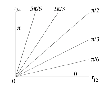
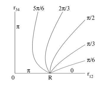
Figure 1: The normalised Higgs field $n$ of the point defect (left) and the monopole loop (right), i.e. before and after deformation. Shown are lines of constant azimuthal angle of $n$ with 0 and $\pi$ standing for the the north and south pole, respectively. Defects are singularities in $n$, where those lines meet. The four-dimensional space-time is visualised by radii $r_{12}^{2}=x_{1}^{2}+x_{2}^{2},\>r_{34}^{2}=x_{3}^{2}+x_{4}^{2}$.

4 Monopole loop as deformation

For configurations near the instanton in configuration space, $A=A_{\rm inst}+\delta A$, one can in principle perform a perturbation theory $\phi=\phi_{\rm inst}+\delta\phi$ à la Schrödinger. Due to lack of knowledge of the full spectrum of the Laplacian this has not been solved. Nevertheless, to investigate the behaviour of the defect, it is sufficient to Taylor expand the perturbation $\delta\phi$ at the defect [2]. For our purposes even the zeroth order will be enough. Without loss of generality we specialise to a perturbation in the third color direction. So finally $\delta\phi=R^{2}\tau_{3}$ since the Higgs field is of dimension (length$)^{2}$.

A straightforward calculation shows that upon this perturbation the defect becomes a monopole loop, namely a circle of radius $R$ in the $x_{1}x_{2}$-plane. This configuration is now generic, the perturbation has (partly) broken the symmetry. The field $n$ with its typical hedgehog behaviour is depicted in Figure 1. It also shows the local nature of the perturbation. The Higgs field is not changed at large distances and still has Hopf invariant 1. Actually the configuration is the one proposed in [1] for the Maximally Abelian gauge, but there it is suppressed by the gauge fixing functional.

What is the precise relation between the monopole loop in the bulk and the Hopf invariant = instanton number at the boundary? It has to do with the twist [7] meaning the rotation of the Higgs field around an axis in color space while moving along the loop. For our case, the polar angle of $n$ depends on the worldline coordinate $\varphi_{12}=\arctan(x_{2}/x_{1})$ and performs just one rotation. Beside the twist, there is the possibility that the instanton number gets contributions from a two-dimensional sheet spanned by the monopole loop [5]. This can be thought of as the set of Dirac strings. The latter will not show up when we discuss the interplay between magnetic charge, twist and instanton number with the help of an auxiliary Abelian fibre bundle in the next section.

5 Auxiliary Abelian fibre bundle

The idea of this section is to describe the properties of the Higgs field $n$ in terms of an auxiliary Abelian gauge field $a$ and its field strength $f={\rm d}a$. These will have immediate physical interpretations. Using the diagonalising gauge transformation of $n$ – the one which transforms the non-Abelian gauge field into the Abelian gauge – these fields have the following expressions,

$$a = (ig{\rm d}g^{\dagger},\tau_{3})\,,\qquad\quad gng^{\dagger}=\tau_{3}\,,$$

$$f = (g{\rm d}g^{\dagger},\tau_{1})\wedge(g{\rm d}g^{\dagger},\tau_{2})=(in,{\rm d}n\wedge{\rm d}n)\,.$$

$a$ is the Abelian projected inhomogeneous part of the gauge transformed non-Abelian field. $f$ is the topological density of $n$, its integral over a two-sphere gives the winding number = magnetic charge. Therefore, these objects carry information about the monopoles in the bulk. On the other hand, they are the ingredients of the Abelian Chern-Simons form $CS(a)=a\wedge f/16\pi^{2}$ which gives the Hopf invariant.

The only subtlety is that $g$ and thus $a$ may not be defined globally (due to topological obstructions) even if $n$ and thus $f$ are. Accordingly, one has to work with patches in the framework of a bundle.

For the base manifold $M$ of this bundle, i.e. the space-time, we have to cut out a tube surrounding the monopole loop, since $n$ is not continuous there. When working on $S^{4}$ one also has to cut out the pole which represents infinity on $\mathbb{R}^{4}$, the transition functions there are genuinely non-Abelian. So, Abelianisation has lead to a space-time $M$ with two boundaries (cf. Figure 2). The outer boundary $\Sigma_{\rm out}=S^{3}_{\infty}$ carries information about the Hopf invariant, the inner boundary $\Sigma_{\rm in}=S^{2}\times S^{1}$ contains the monopole loop.

$n$ is smooth over $M$ by definition. Its diagonalisation will be smooth only over patches $U_{i}$, $g_{i}ng^{\dagger}_{i}=\tau_{3}$. The local gauge field reads $a_{i}=(ig_{i}{\rm d}g^{\dagger}_{i},\tau_{3})$. Indeed, the residual gauge freedom $g\rightarrow\exp(i\lambda\tau_{3})g$ transforms it as $a\rightarrow a+{\rm d}\lambda$. In particular the transition on the overlap of two patches is $a_{i}=a_{j}+{\rm d}\lambda_{ij}$.

The key point in the construction is the vanishing of the topological density $f\wedge f$ due to its form content. As will be explained now, the zero instanton number of the auxiliary field interpolates between the boundaries. In a way, our method is similar to the residue calculus.

Figure 2: The construction of the base manifold $M$ by cutting out the monopole loop (and infinity) and its minimal patching with $U_{1}$ and $U_{2}$. The contribution of the monopole loop to the (vanishing) instanton number reduces finally to the shown two-torus.

It is well-known, that the instanton number can be expressed in terms of transition functions $\Omega_{ij}$ [8]. For the case of a non-Abelian theory without boundaries the formula reads,

$$\nu(A)=\frac{1}{48\pi^{2}}\sum_{i,j}\int_{U_{i}\cap U_{j}}\!\!\!\!\rm tr\>(\Omega_{ij}^{\dagger}{\rm d}\Omega_{ij})^{3}+\frac{1}{48\pi^{2}}\sum_{i,j,k}\int_{U_{i}\cap U_{j}\cap U_{k}}\!\!\!\!\rm tr\>(\Omega_{ij}{\rm d}\Omega_{ij}^{\dagger}\wedge{\rm d}\Omega_{jk}^{\dagger}\Omega_{jk})\,,$$

where we have suppressed orientations. Abelian transition functions can only contribute to the second term. We note in passing that for Abelian instantons on the four-torus these are integrals over two-tori.

For a manifold with boundaries one has to include two more terms,

$$0=\nu(a)= \!\!\!\!\!-\frac{1}{96\pi^{2}}\sum_{i,j,k}\int_{U_{i}\cap U_{j}\cap U_{k}}{\rm d}\lambda_{ij}\wedge{\rm d}\lambda_{jk}$$

$$\!\!\!\!\!+\frac{1}{16\pi^{2}}\sum_{i}\int_{U_{i}\cap\Sigma}a_{i}\wedge f+\frac{1}{32\pi^{2}}\sum_{i,j}\int_{U_{i}\cap U_{j}\cap\Sigma}a_{i}\wedge{\rm d}\lambda_{ij}\,.$$

The new terms are boundary contributions with a similar structure, but not entirely given in terms of transition functions. They will be interpreted in terms of the Hopf invariant and monopole properties. The old term is not of this form but only occurs for more than two patches. Therefore we continue with the search for a minimal patching of $M$.

How big are the subspaces $U_{i}$ of $M$ on which on can define a smooth diagonalisation $g_{i}$? In other words, given a smooth field strength $f$ fulfilling the Bianchi identity $df=0$, on which $U_{i}$ can one define smooth $a_{i}$ with $f={\rm d}a_{i}$? The answer is the second cohomology $H^{2}(U_{i})$. Loosely speaking, the patches $U_{i}$ need not be contractable but are not allowed to have two-dimensional holes.

For a strip near the inner boundary we have $H^{2}(S^{2}\times S^{1}\times\mbox{interval})\neq 0$. The $S^{2}$-factor gives the magnetic charge. This $S^{2}$ needs to be divided into two patches for every point on the worldline $S^{1}$. This fact is well-known from the Wu-Yang construction of the Dirac monopole avoiding Dirac strings. One of the patches should contain the points where $n$ points say southwards.

For a strip near the outer boundary we have $H^{2}(S^{3}\times\mbox{interval})=0$. Therefore this volume can be covered with just one patch, a fact that plays a role in the definition of the Hopf invariant.

One can match the patches discussed so far in such a manner, that the minimal atlas of $M$ consists of two patches, see Figure 2. Firstly, extend the south patch of the monopole to a thick sheet $U_{1}$ spanned by the loop. Secondly, glue the other patch $U_{2}$ of the monopole with the patch at the outer boundary. In this way the instanton number will not pick up the mentioned bulk contributions and the instanton topology is ‘localised’ on the boundary of the monopole tube.

The final step will be the interpretation of the boundary contributions. This is very easy at the outer boundary. Since it is covered by one patch, only the second term in the above formula will contribute. Moreover, it perfectly coincides with the Hopf invariant. At the inner boundary the second term can be further reduced due to the third cohomology. The whole contribution of this boundary reduces to a two-torus $U_{1}\cap U_{2}\cap\Sigma_{\rm in}$ like for the Abelian instantons. Moreover, the integral factorises into two integrals over circles. The first one is the integral of ${\rm d}\lambda_{12}$ over an $S^{1}$ around the loop which is nothing but the magnetic charge. The second one is an integral of the gradient of the polar angle of $n$ over an $S^{1}$ along the loop. In Section 4 we have identified this as the twist. Thus we arrive at the simple formula

instanton number = Hopf invariant = magnetic charge $$\times$$ twist

which is a special case of the complicated one discussed in [5]. For the case at hand we have $1=1=1\times 1$.

6 Summary and Outlook

We have discussed the defects induced by instantons in the Laplacian Abelian gauge. The single instanton leads to a non-generic point defect. The latter is a seed for a monopole loop (or a monopole loop ‘shrunken to zero radius’). A perturbation of the background makes this monopole visible. In addition, the monopole loop comes with a twist. It can be viewed as generating the electric field needed for the instanton number. We emphasize that details of the monopole loop like its position depend on the chosen Abelian gauge.

The topological considerations, however, are gauge-independent. The instanton number is converted into the Hopf invariant of the normalised Higgs field $n$. Measured on the boundary, it can be related to the properties of the monopole in the bulk. For this purpose we have introduced an auxiliary Abelian fibre bundle. It avoids singularities like Dirac strings. The task in this approach is to find a (minimal) patching and to compute and interpret the remaining boundary terms. In a very transparent way this leads to the instanton number being the product of magnetic charge and twist. This method is valid for any configuration in any Abelian gauge. In principle it can also be applied to other space-times like tori, where however the patching will be different. The twist has also been found for the constituent monopoles of calorons.

Topology can only describe the kinematics of monopoles. One might still speculate, that the shown correlation between instantons and monopoles may have implications for the dynamics. This will certainly be the case when modelling the QCD vacuum as an instanton ensemble. The instanton liquid has been successful for chiral symmetry breaking. However, confinement could not be explained by a reasonable instanton ensemble so far. It has been observed that the individual monopole loops of two and more instantons are able to fuse to one larger one. This suggests that under certain circumstances a percolating monopole loop can be generated in this way.

7 Acknowledgements

The author thanks the organisers for a stimulating workshop in a nice surrounding. Furthermore he is grateful to Alexander Bais, Philippe de Forcrand, Michael Engelhardt, Chris Ford, Oliver Jahn and Pierre van Baal for helpful discussions. This work was supported by FOM.

We use half the Pauli matrices $\tau_{a}=\sigma_{a}/2$ as the basis in color space, i.e. as the generators of the Lie algebra $su(2)$. The scalar product of vectors is $(x,y)=2\,\rm tr\>xy=x_{a}y_{a}$, where $x=x_{a}\tau_{a}$. The wedge product of ‘colored differential forms’ is defined accordingly $x\wedge y=i/2\,\epsilon_{abc}\,x_{a}\wedge y_{b}\,\tau_{c}$.

The Hopf invariant can be defined as a linking number. An algebraic definition starts with a two-form $f=(in,{\rm d}n\wedge{\rm d}n)$. Because $f$ is closed and the second cohomology of $S^{3}$ vanishes, there exists a one-form $a$ with ${\rm d}a=f$. Together, these forms built a three-form to integrate over, and $H(n)=\int_{S^{3}}a\wedge f/16\pi^{2}$.

This construction can be rewritten in terms of the diagonalising gauge transformation, cf. Section 5. The Hopf invariant $H(n)=\int_{S^{3}}\rm tr\>(g{\rm d}g^{\dagger})^{3}/24\pi^{2}$ becomes the winding number of $g$, in the usual sense of a mapping from $S^{3}$ to $SU(2)\cong S^{3}$.

References

- [1] Brower, R. C., Orginos, K. N. and Tan, C.-I. (1997) Magnetic monopole loop for the Yang-Mills instanton, Phys. Rev., D55, pp. 6313–6326
- [2] Bruckmann, F. (2001) Hopf defects as seeds for monopole loops, J. High Energy Phys., 0108, p. 30
- [3] Bruckmann, F., Heinzl, T., Vekua, T. and Wipf, A. (2001) Magnetic Monopoles vs. Hopf Defects in the Laplacian (Abelian) Gauge, Nucl. Phys., B593, pp. 545–561
- [4] de Forcrand, P., private communication.
- [5] Jahn, O. (2000) Instantons and monopoles in general Abelian gauges, J. Phys., A33, pp. 2997–3019
- [6] ’t Hooft, G. (1981) Topology of the Gauge Condition and New Confinement Phases in Non-Abelian Gauge Theories, Nucl. Phys., B190, pp. 455
- [7] Taubes, C. H. (1984) Morse theory and monopoles: Topology in long-ranged forces, in G. ’t Hooft (ed.) Progress in gauge field theory, Plenum Press, New York
- [8] van Baal, P. (1982) Some Results for SU(N) Gauge Fields on the Hypertorus, Commun. Math. Phys., 85, pp. 529
- [9] van der Sijs, A. J. (1997) Laplacian Abelian projection, Nucl. Phys. B (Proc. Suppl.), 53, pp. 535–537