QMUL-PH-02-08

hep-th/0204228

F-theory duals of M-theory on $S^{1}/\mathbb{Z}_{2}\times T^{4}/\mathbb{Z}_{N}$

Monika Marquart^1,2 and Daniel Waldram^2,3

¹Fachbereich Physik, Martin-Luther-Universität Halle-Wittenberg
Friedemann-Bach-Platz 6,
D-06099 Halle, Germany

²Department of Physics
Queen Mary, University of London
Mile End Rd, London E1 4NS, UK

³Isaac Newton Institute for Mathematical Sciences
University of Cambridge
20 Clarkson Road, Cambridge, CB3 0EH, U.K.

Abstract

In this note, we use results of Aspinwall and Morrison to discuss the F-theory duals of certain $T^{4}/\mathbb{Z}_{N}$ orbifold compactifications of Hořava–Witten theory. In the M-theory limit an interesting set of rules, based on anomaly cancellation, has been developed for what gauge and matter multiplets must be present on the various orbifold fixed planes. Here we show how several aspects of these rules can be understood directly from F-theory.

1 Introduction

The description of orbifold compactifications of M-theory began with the seminal paper of Hořava and Witten [1] which realised the strongly coupled $E_{8}\times E_{8}$ heterotic string as eleven-dimensional M-theory compactified on $S^{1}/\mathbb{Z}_{2}$. Subsequently, a number of authors have considered other orbifold compactifications. Models based on orbifolds of $T^{5}$ were considered in [2] and [3, 4] (see also [5]). More recently, two groups [6, 7] have made a general analysis of Hořava–Witten type compactifications on spaces of the form $S^{1}/\mathbb{Z}_{2}\times Y$, where $Y=T^{4}/\mathbb{Z}_{N}$ is an orbifold limit of K3. These models preserve $\mathcal{N}=1$ supersymmetry in six dimensions, and have a weak-coupling limit given by the heterotic string compactified on $Y$.

Since there is no fundamental formulation of M-theory, in each case, following [1], it has been necessary to use consistency arguments, in particular the requirements of anomaly cancellation, to deduce what twisted matter and interactions reside on the orbifold fixed planes. This has led particularly the authors of [6] and also of [7] to derive a very interesting and complete set of rules for constucting such models. These are, in general, far from intuitive from a geometrical perspective. One way to understand this is that there are necessarily large M-theory corrections to the geometry near the orbifold fixed planes. The rules are of particular interest because they can be generalised to describe supersymmetric orbifold compactifications to four-dimensions [8] which may provide interesting new avenues for model-building.

Recently, it has been possible to justify the rules developed in [6, 7] by considering duality to type I’ superstring compactifications [9]. Here, we take an alternative approach, using results of Aspinwall and Morrison [10, 11] to describe the compactifications by their F-theory duals. These results are not new, but by taking the M-theory limit with $Y$ large [12, 10] one gets a simple understanding of several of the rules developed in [6, 7]. (An obvious complementary approach would be to use the toric description of the F-theory models as for instance in [13].) We concentrate on the example where $Y=T^{4}/\mathbb{Z}_{2}$ and the $E_{8}$ gauge bundles are such that a perturbative $\operatorname{\mathit{SO}}(16)\times[\operatorname{\mathit{SU}}(2)\times E_{7}]$ subgroup is preserved. This model has the interesting property of matter charged under groups from both $E_{8}$ ten-planes. In the final section, we discuss generalisations to F-theory limits of compactifications with various other bundles and orbifolds.

2 Hořava–Witten theory on $Y=T^{4}/\mathbb{Z}_{N}$

We start by reviewing the description of orbifold compactifications of Hořava–Witten theory on $Y$ following the work of [6] and [7]. For definiteness, we will concentrate on the duals of perturbative heterotic models on $Y=T^{4}/\mathbb{Z}_{2}$, though at the end of the paper we will briefly consider other orbifold limits of K3 and gauge groups.

2.1 Heterotic string limit, orbifolds and fractional instantons

First, consider the $E_{8}\times E_{8}$ heterotic string compactified on $Y$. If $Y=T^{4}/\mathbb{Z}_{2}$, the orbifold has sixteen fixed points, each giving an $A_{1}$ singularity where the geometry is locally $\mathbb{C}^{2}/\mathbb{Z}_{2}$. For the gauge fields in perturbative backgrounds, one typically assumes that the gauge bundle on the unquotiented space $T^{4}$ is flat and then makes some identification of the gauge bundle fibres under the $\mathbb{Z}_{2}$ orbifold action. The bundle on $Y$ then has, at most, $\mathbb{Z}_{2}$ holonomy around the $A_{1}$ singularities. Any field strength is localized at the singularity and if the holonomy is non-trivial, this gives a “fractional instanton” [14], with possibly non-integral instanton charge.

There are basically three possibilities for embedding the $\mathbb{Z}_{2}$ holonomy in $E_{8}$: it can be trivial, in which case the unbroken gauge symmetry remains $E_{8}$, it can break $E_{8}$ to $\operatorname{\mathit{Spin}}(16)/\mathbb{Z}_{2}$, or it can break $E_{8}$ to $[\operatorname{\mathit{SU}}(2)\times E_{7}]/\mathbb{Z}_{2}$. (These latter two we will refer to loosely as $\operatorname{\mathit{SO}}(16)$ and as $\operatorname{\mathit{SU}}(2)\times E_{7}$.)

For perturbative backgrounds two possibilities arise [15, 16]. Either one $E_{8}$ is trivial while the other is broken so the final symmetry is $E_{8}\times[\operatorname{\mathit{SU}}(2)\times E_{7}]$, or both are broken giving $\operatorname{\mathit{SO}}(16)\times[\operatorname{\mathit{SU}}(2)\times E_{7}]$. The former case is the so called “standard embedding”. In this note, we will concentrate on the latter case. One can calculate the fractional instanton charge at each $A_{1}$ singularity associated with the given $\mathbb{Z}_{2}$-bundle. One finds that for the latter case, each fractional instanton giving the $\operatorname{\mathit{SO}}(16)$ factor has charge one. For the $\operatorname{\mathit{SU}}(2)\times E_{7}$ factor, on the other hand, each fractional instanton has charge $1/2$. For the standard embedding the corresponding instantons also have charge $3/2$. Thus in both cases the net charge per singularity is $3/2$.

An important requirement of heterotic compactifications is that, as a result of anomaly cancellation, the net “magnetic charge”, as given by $\operatorname{c}_{2}(V_{1})+\operatorname{c}_{2}(V_{2})-\operatorname{c}_{2}(TY)$, must vanish. Here $\operatorname{c}_{2}(V_{1})+\operatorname{c}_{2}(V_{2})$ is the total gauge instanton charge given by the sum of the second Chern classes of the two $E_{8}$ gauge bundles $V_{1}$ and $V_{2}$. The last term is the second Chern class of the tangent bundle of the compact manifold $Y$, with $\operatorname{c}_{2}(TY)=24$ for a K3 surface. Thus if $Y$ is a $T^{4}/\mathbb{Z}_{2}$ orbifold, the last term gives a contribution of $-24/16=-3/2$ for each $A_{1}$ singularity. Consequently the net gauge instanton number per singularity must be $3/2$ as is indeed the case for the two perturbative examples discussed above.

The full spectrum of the theory is given in [15, 16]. For our main example the unbroken gauge group is $\operatorname{\mathit{SO}}(16)\times[\operatorname{\mathit{SU}}(2)\times E_{7}]$. Given $\mathcal{N}=1$ supersymmetry in six dimensions, we can expect matter in hypermultiplets or tensor multiplets as well as the gauge vector multiplets. The breaking $E_{8}\to\operatorname{\mathit{SO}}(16)$ leads to a decomposition $\mathbf{248}\to(\mathbf{120}+\mathbf{128})$. This gives the $120$ vector multiplets transforming in the adjoint representation and $128$ hypermultiplets transforming in the spinor representation of $SO(16)$. Meanwhile the breaking $E_{8}\to\operatorname{\mathit{SU}}(2)\times E_{7}$ leads to a decomposition $(\bf{248})\to(\mathbf{1},\mathbf{133})+(\mathbf{3},\mathbf{1})+(\mathbf{2},\mathbf{56})$. The first two factors give the $133$ vector multiplets in the adjoint representation of $E_{7}$ and three vector multiplets in the adjoint representation of $SU(2)$. The third factor gives $112$ hypermultiplets in the bifundamental representation. In addition the compactification leads to four moduli which are hypermultiplets and gauge singlets and there is one universal tensor multiplet which includes the dilaton. Thus far this is just the untwisted massless spectrum of the weakly coupled heterotic theory. In addition there are twisted string states on the $T^{4}/\mathbb{Z}_{2}$ orbifold. These give sixteen half hypermultiplets transforming as $\frac{1}{2}(\mathbf{16},\mathbf{2},\mathbf{1})$ and so are charged under both factors in the perturbative gauge group $E_{8}\times[\operatorname{\mathit{SU}}(2)\times E_{7}]$.

2.2 Hořava–Witten geometry

Hořava–Witten theory gives the strong coupling limit of the $E_{8}\times E_{8}$ heterotic string as M-theory compactified on $S^{1}/\mathbb{Z}_{2}$. Thus here our starting point is M-theory compactified on the product of two $\mathbb{Z}_{2}$ orbifolds $T^{4}/\mathbb{Z}_{2}\times S^{1}/\mathbb{Z}_{2}$. The orbifold projection acting on $S^{1}$ leaves two fixed ten-planes. Following Hořava and Witten, there are $E_{8}$ vector multiplets localized on each fixed ten plane. The action of the $\mathbb{Z}_{2}$ on $T^{4}$ leaves sixteen fixed seven-planes. The combined action of both orbifolds results in sixteen pairs of fixed six-planes, which are the intersections of the two fixed ten-planes and the sixteen fixed seven-planes.

In general, one expects additional gauge and matter degrees of freedom on the fixed seven- and six-planes. The compactification of M-theory on $T^{4}/\mathbb{Z}_{2}$ gives a theory with sixteen supercharges so that the only possible multiplets on the fixed seven-planes are seven-dimensional vectors. Compactifying further on $S^{1}/\mathbb{Z}_{2}$ breaks half of the supersymmetry to eight supercharges. Thus we can have six-dimensional hypermultiplets or vector multiplets on the fixed six-planes.

A priori, since there is no fundamental formulation of M-theory it is unclear what new multiplets appear. However, following Hořava and Witten, the new degrees of freedom can be deduced from the requirement of anomaly cancellation [6, 7]. On the six-dimensional planes this is a particularly powerful tool as there are gauge, gravitational and mixed anomalies. Since there are no chiral anomalies in odd dimensions, it would appear to be impossible to determine the matter content on the seven-planes. However, by considering those parts of the seven-dimensional multiplets which survive the $\mathbb{Z}_{2}$ projection onto the six-planes, in turns out that the six-dimensional anomalies are basically sufficient to determine the seven-dimensional content.

These kinds of arguments have led to a set of local rules for what matter and gauge groups are present on each fixed plane for different $T^{4}/\mathbb{Z}_{N}$ orbifolds [6, 7]. In particular, one finds the following for the perturbative $\operatorname{\mathit{SO}}(16)\times[\operatorname{\mathit{SU}}(2)\times E_{7}]$ model. First, one assumes the $E_{8}$ bundles on the two fixed ten-planes have the same $\mathbb{Z}_{2}$ holonomies as in the weakly coupled string limit, so again there are fractional instantons localised on the six-planes, giving an unbroken perturbative $\operatorname{\mathit{SO}}(16)\times[\operatorname{\mathit{SU}}(2)\times E_{7}]$ gauge group. The familiar untwisted states of the string theory limit then appear as zero-modes of the $E_{8}$ vector multiplets in this background. Anomaly cancellation implies that there must be $\operatorname{\mathit{SU}}(2)$ vector multiplets on each of the fixed seven-planes. This is as expected given that these give planes of $A_{1}$ singularities, so the geometrical blow-up modes together with wrapped M2-brane states should form an $\operatorname{\mathit{SU}}(2)$ gauge multiplet. Naively one would expect these to be new non-perturbative degrees of freedom so the full low-energy gauge symmetry becomes

$$\operatorname{\mathit{SO}}(16)\times[\operatorname{\mathit{SU}}(2)\times E_{7}]\times\operatorname{\mathit{SU}}(2)_{\text{non-pert}}^{16}.$$ (2.1)

An important issue is how to identify the twisted string states which are charged under both the perturbative $\operatorname{\mathit{SO}}(16)$ and $\operatorname{\mathit{SU}}(2)$ groups. The problem is that in Hořava–Witten theory these live on different separated fixed ten-planes, and so it appears no localised state could be charged under both factors.

The minimal solution to this problem, consistent with anomaly cancellation, was given in [6] and [7]. The point is that, on each of the six-planes where the sixteen seven-planes intersect $\operatorname{\mathit{SU}}(2)\times E_{7}$ ten-plane, one must identity the non-perturbative seven-dimensional $\operatorname{\mathit{SU}}(2)$ gauge fields with the perturbative $\operatorname{\mathit{SU}}(2)$ fields. This correlates gauge transformations on the two factors so in the language of [6] there is simply a single $\operatorname{\mathit{SU}}(2)$ gauge group extending over one ten-plane and the sixteen seven-planes. In [7], this “locking” of the gauge groups is characterised by saying that the gauge factor visible in the heterotic string description is the diagonal $\operatorname{\mathit{SU}}(2)^{*}=\operatorname{diag}(\operatorname{\mathit{SU}}(2)\times\operatorname{\mathit{SU}}(2)^{16}_{\text{non-pert}})$ of the product of the non-perturbative and perturbative groups. Both papers [6] and [7] identify the low-energy six-dimensional gauge group as having a single $\operatorname{\mathit{SU}}(2)$ factor

$$\operatorname{\mathit{SO}}(16)\times[\operatorname{\mathit{SU}}(2)^{*}\times E_{7}].$$ (2.2)

Here we will interpret this as implying that the zero modes for the gauge fields of this single $\operatorname{\mathit{SU}}(2)^{*}$ factor extend over both one fixed ten-plane and the sixteen fixed seven-planes. It is then argued that the twisted matter lives on the other set of six-planes where the seven-planes intersect the $\operatorname{\mathit{SO}}(16)$ ten-plane. The matter is charged under the non-perturbative $\operatorname{\mathit{SU}}(2)$ factor, but because of the locking this means it is, in fact, also charged under the single perturbative $\operatorname{\mathit{SU}}(2)$ on the other ten-plane (essentially because the zero mode extends over both the ten- and seven-planes). This explains how the twisted matter can be both local and carry the correct charge.

One other, counter-intuitive related rule is required in order to cancel all the anomalies. Naively one expects the fields $\Phi_{i}$ of the seven-dimensional vector multiplets to have definite transformation properties under the $S^{1}/\mathbb{Z}_{2}$ orbifold projection: so that $\Phi_{i}(x^{11})=\Phi_{i}(-x^{11})$ or $\Phi_{i}(x^{11})=-\Phi_{i}(-x^{11})$. In general, the seven-dimensional vector multiplet splits into a vector multiplet and a hypermultiplet in six-dimensions. Under the projection one expects one or other of these multiplets to remain massless. Remarkably the anomaly rules require that, in general, one must allow for different parts of the seven-dimensional vector multiplet to survive the projection to each of the two six-planes at the intersections of the fixed seven- and ten-planes.

This is very unexpected, since, if the compact space is really $T^{4}/\mathbb{Z}_{2}\times S^{1}/\mathbb{Z}_{2}$, then we would expect the seven-dimensional fields to have definite transformation properties and the same part of the multiplet would survive on each six-plane. Similarly, it is hard to understand, purely geometrically, why one should identify the perturbative and apparently non-perturbative gauge groups as a single $\operatorname{\mathit{SU}}(2)^{*}$ factor.

The solution is that the compact space cannot in fact be a product. The presence of magnetic charges at each $A_{1}$ singularity acts as a source which necessarily distorts the space. The point is that in Hořava–Witten theory the gauge fields and Riemann curvature on each ten-plane $M_{1}$ and $M_{2}$ couple magnetically to the four-form $G$ of the bulk eleven-dimensional supergravity [1] (as well as providing a source of stress-energy in Einstein’s equations [17]). One has

$$\mathrm{d}G\sim m_{P}^{-3}\left[\operatorname{tr}(F_{1}\wedge F_{1})-\frac{1}{2}\operatorname{tr}(R\wedge R)\right]\wedge\delta(M_{1})\\ +m_{P}^{-3}\left[\operatorname{tr}(F_{2}\wedge F_{2})-\frac{1}{2}\operatorname{tr}(R\wedge R)\right]\wedge\delta(M_{2}),$$ (2.3)

where $F_{1}$ and $F_{2}$ are the two $E_{8}$ gauge field strengths and $m_{P}$ is the eleven-dimensional Planck mass. Note that the integral of the right-hand side of the equation over $S^{1}/\mathbb{Z}_{2}\times Y$ gives the net magnetic charge $\operatorname{c}_{2}(V_{1})+\operatorname{c}_{2}(V_{1})-\operatorname{c}_{2}(TY)$ which we know from above vanishes, as it must since $\mathrm{d}G$ is exact. However, the sources in general do not cancel at every point. For instance, in the orbifold compactifications all the $\operatorname{tr}(F_{i}\wedge F_{i})$ and $\operatorname{tr}(R\wedge R)$ charge is localised at the orbifold singularities, and is proportional to the corresponding contributions to the second Chern classes. These need not cancel at each $A_{1}$ singularity on each ten-plane separately. In particular, we see that there is a net charge on the $\operatorname{\mathit{SO}}(16)$ ten-plane of $-1/4$ per $A_{1}$ singularity, and a net charge on the $\operatorname{\mathit{SU}}(2)\times E_{7}$ ten-plane of $+1/4$ per $A_{1}$ singularity. As a result $G\neq 0$ in the eleven-dimensional bulk and, as in [18], the manifold deforms from a simple product. For smooth compactifications one can suppress this effect by choosing $Y$ to be very large and the gauge fields slowly varying so that the sources are small with respect to $m_{P}$. However, in the orbifold limit, there is no scale to the curvature of $Y$ or the gauge field strength since both are singular and there is no analogous suppression.

In summary, aside from [9], there has been no derivation of the M-theory rules [6, 7] from first principles. It is only possible to show that the anomalies cancel using this recipe. It may be possible to gain additional insight by considering the full deformed M-theory geometry, in particular, how this could lead to the identification of $\operatorname{\mathit{SU}}(2)$ factors and the projections on the seven-dimensional multiplets. Here, instead, we will consider the F-theory duals to justify the rules, though note this will also provide additional evidence that the M-theory background is deformed.

3 F-theory description

In this section we consider the F-theory formulation of the $SO(16)\times[E_{7}\times SU(2)]$ model. We will see that the matter content and gauge groups can be derived directly. In particular, we justify the identification of a heterotic $SU(2)^{*}$ gauge group and the appearance of twisted matter states discussed at the end of the last section. We should point out that these F-theory models are not new but are a simple case of a class of models considered in [11]. The results are briefly generalized to other models in the next section.

3.1 F-theory and the stable degeneration limit

Let us first summarize the duality in six dimensions between F-theory compactified on a Calabi-Yau threefold $X$ and the heterotic string compactified on an elliptically fibred K3 surface $Y$ [19]. To keep the problem as simple as possible we restrict ourselves to describing the classical geometry of $Y$, which means that both the base $\mathbb{P}^{1}_{B}$ and the elliptic fibre of $Y$ are large. This corresponds on the F-theory side to taking a particular limit of the threefold known as a stable degeneration, first discussed in [20] and explained in detail in [10].

Recall that under the duality, the elliptic fibers of the heterotic K3 manifold $Y$ are replaced by K3 fibers in the F-theory threefold $X$. These fibers are themselves elliptically fibred so that $X$ can be viewed as an elliptic fibration over a Hirzebruch surface $\pi:X\to\mathbb{F}_{n}$. The Hirzebruch surface itself is a $\mathbb{P}^{1}$ fibration over the common base $\mathbb{P}^{1}_{B}$, giving a projection $\mathbb{F}_{n}\to\mathbb{P}^{1}_{B}$.

The elliptic fibration $\pi:X\to\mathbb{F}_{n}$, which, by definition, also has a section $\sigma:\mathbb{F}_{n}\to X$, can be described via a Weierstrass model

$$y^{2}=x^{3}+a(s,t)x+b(s,t),$$ (3.1)

where $s$ and $t$ parametrise the base $\mathbb{P}^{1}_{B}$ and the fibre $\mathbb{P}^{1}$ of $\mathbb{F}_{n}$. The affine coordinates $x$ and $y$ are sections of $\mathcal{L}^{2}$ and $\mathcal{L}^{3}$ respectively where $\mathcal{L}$ is the co-normal bundle to the $\mathbb{F}_{n}$ section in $X$. Similarly $a$ and $b$ are sections of $\mathcal{L}^{4}$ and $\mathcal{L}^{6}$. Since $X$ is Calabi–Yau, the canonical bundle $K_{X}$ is trivial, so that, by adjunction, $\mathcal{L}=K_{\mathbb{F}_{n}}^{-1}$. The torus degenerates whenever the discriminant $\delta=24b^{2}+4a^{3}$, which is a section of $\mathcal{L}^{12}$, vanishes. These degenerations characterise the enhanced gauge symmetries of the theory, following the classical Kodaira classification. The gauge group at a given point in the base is determined by the order of vanishing of the sections $\delta$, $a$ and $b$ as summarized the familiar list given in Table 1 taken from [10].

$o(a)$	$o(b)$	$o(\delta)$	Kodaira fibre	singularity	gauge algebra
$\geq 0$	$\geq 0$	0	$\operatorname{\mathit{I}}_{0}$	-	-
0	0	1	$\operatorname{\mathit{I}}_{1}$	-	-
0	0	$2n\geq 2$	$\operatorname{\mathit{I}}_{2n}$	$A_{2n-1}$	$\operatorname{\mathit{su}}(2n)$ or $\operatorname{\mathit{sp}}(2n)$
0	0	$2n+1\geq 3$	$\operatorname{\mathit{I}}_{2n+1}$	$A_{2n}$	$\operatorname{\mathit{su}}(2n+1)$ or $\operatorname{\mathit{so}}(2n+1)$
$\geq 1$	1	2	$\operatorname{\mathit{II}}$	-	-
1	$\geq 2$	3	$\operatorname{\mathit{III}}$	$A_{1}$	$\operatorname{\mathit{su}}(2)$
$\geq 2$	2	4	$\operatorname{\mathit{IV}}$	$A_{2}$	$\operatorname{\mathit{su}}(3)$ or $\operatorname{\mathit{su}}(2)$
$\geq 2$	$\geq 3$	6	$\operatorname{\mathit{I}}_{0}^{*}$	$D_{4}$	$\operatorname{\mathit{so}}(8)$ or $\operatorname{\mathit{so}}(7)$ or $g_{2}$
2	3	$n+6\geq 7$	$\operatorname{\mathit{I}}_{n}^{*}$	$D_{n+4}$	$\operatorname{\mathit{so}}(2n+8)$ or $\operatorname{\mathit{so}}(2n+7)$
$\geq 3$	1	8	$\operatorname{\mathit{IV}}^{*}$	$E_{6}$	$e_{6}$ or $f_{4}$
3	$\geq 5$	9	$\operatorname{\mathit{III}}^{*}$	$E_{7}$	$e_{7}$
$\geq 4$	5	10	$\operatorname{\mathit{II}}^{*}$	$E_{8}$	$e_{8}$
$\geq 4$	$\geq 6$	$\geq 12$	non-minimal

Table 1: Orders of vanishing, fibres, singularities and gauge algebra

If we write $L$ for the class of divisors associated to the vanishing of sections of $\mathcal{L}$, since $\mathcal{L}=K_{\mathbb{F}_{n}}^{-1}$ we have

$$L=2C_{0}+(n+2)f,$$ (3.2)

where $C_{0}$ is the class of the exceptional divisor on $\mathbb{F}_{n}$ and $f$ the class of the $\mathbb{P}^{1}$ fibre of $\mathbb{F}_{n}\to\mathbb{P}^{1}_{B}$. These form a basis of divisor classes on $\mathbb{F}_{n}$ and have intersections $C_{0}\cdot C_{0}=-n$, $C_{0}\cdot f=1$ and $f\cdot f=0$. The discriminant curve $\Delta$ defined by $\delta=0$ is in the class $\Delta=12L$.

Now we turn to the stable degeneration limit introduced in [20, 10]. In the limit where the heterotic K3 manifold $Y$ is taken to the large, the $\mathbb{P}^{1}$ fibre of the F-theory $\mathbb{F}_{n}$ base degenerates into a pair of intersecting $\mathbb{P}^{1}$ curves. This can be viewed as one $S^{1}$ cycle in the two-sphere $\mathbb{P}^{1}$ pinching to a point. The F-theory base then degenerates into a pair of Hirzebruch surfaces, $\mathbb{F}_{n,1}$ and $\mathbb{F}_{n,2}$, intersecting over a $\mathbb{P}^{1}$ curve $C_{*}$. This is a section in the class $C_{*}=C_{0}+nf$ on each $\mathbb{F}_{n}$ surface. The full F-theory threefold $X$ is a degeneration into a pair of threefolds $X_{1}$ and $X_{2}$ intersecting in a K3 surface, which is the elliptic fibration over $C_{*}$. This is shown in Figure 1.

Figure 1: The stable degeneration of $X$

The intersection K3 surface can then be identified with the heterotic K3 surface $Y$. Roughly, one can identify each threefold with one $E_{8}$ group of the heterotic string. Because of the degeneration, the elliptically fibred threefolds $\pi_{1}:X_{1}\to\mathbb{F}_{n,1}$ and $\pi_{2}:X_{2}\to\mathbb{F}_{n,2}$ are no longer Calabi–Yau. Instead, the canonical bundles pick up a contribution from the pull-back of $C_{*}$, so that, as classes, $K_{X_{1}}=\pi_{1}^{*}(C_{*})$ and $K_{X_{2}}=\pi_{2}^{*}(C_{*})$. Consequently, the class $L$ of the co-normal bundle $\mathcal{L}$ on each threefold is now given by $L=-(K_{\mathbb{F}_{n,1}}+C_{*})$, so that

$$L=C_{0}+2f$$ (3.3)

on each of $\mathbb{F}_{n,1}$ and $\mathbb{F}_{n,1}$. As before, in the Weierstrass model of $X_{1}$ and $X_{2}$, the polynomials $a$, $b$ and $\delta$ are still sections of $\mathcal{L}^{4}$, $\mathcal{L}^{6}$ and $\mathcal{L}^{12}$ respectively.

3.2 The $\operatorname{\mathit{SO}}(16)\times[\operatorname{\mathit{SU}}(2)\times E_{7}]$ model

We now discuss the particular F-theory geometry corresponding to the perturbative $\operatorname{\mathit{SO}}(16)\times[\operatorname{\mathit{SU}}(2)\times E_{7}]$ model. By restricting ourselves to the Weierstrass model (3.1) we naturally describe a different $\mathbb{Z}_{2}$-orbifold limit of the heterotic K3 from $T^{4}/\mathbb{Z}_{2}$. However, it is only the local geometry near each $A_{1}$ singularity which encodes the information relevant to the M-theory rules and so this model is quite sufficient. In fact, it is relatively easy to generalize the discussion to get the full global $T^{4}/\mathbb{Z}_{2}$ model if required.

Recall that the $E_{8}$ gauge bundles in the heterotic limit had discrete $\mathbb{Z}_{2}$ holonomy. The F-theory duals of such models have been described explicitly by Aspinwall and Morrison [11]. The following discussion is the direct analogue of their $\mathbb{Z}_{3}$ example.

Requiring that we have $\mathbb{Z}_{2}$ holonomy restricts the polynomials $a$, $b$ in the Weierstrass model to have a particular form given by

$$a =a_{4}-\frac{1}{3}a_{2}^{2},$$ (3.4)

$$b =\frac{1}{27}a_{2}\left(2a_{2}^{2}-9a_{4}\right),$$

$$\delta =a_{4}^{2}\left(4a_{4}-a_{2}^{2}\right)$$

where $a_{i}$ is a section of $\mathcal{L}^{i}$. Recall that the two possible preserved gauge groups for a $\mathbb{Z}_{2}$-bundle in $E_{8}$ are $\operatorname{\mathit{SO}}(16)$ and $\operatorname{\mathit{SU}}(2)\times E_{7}$. From the Table 1 we expect these to correspond to Kodaira fibres of type $\operatorname{\mathit{I}}^{*}_{4}$ and $(\operatorname{\mathit{I}}_{2}+\operatorname{\mathit{III}}^{*})$ respectively.

Let us first consider the threefold $X_{1}$ with gauge group $\operatorname{\mathit{SO}}(16)$. Following the usual prescription the unbroken perturbative gauge group is given by singular fibers over the exceptional divisor $C_{0}$ on $\mathbb{F}_{n,1}$. Let $c_{0}=0$ define this divisor. For $\operatorname{\mathit{SO}}(16)$ we need $\operatorname{\mathit{I}}^{*}_{4}$ fibres, so, from Table 1, we see that the polynomials $a,b$ and $\delta$ vanish to orders $2,3$ and $10$ on $C_{0}$. This implies that the polynomials $a_{2}$ and $a_{4}$ have to be of the form

$$a_{2}=c_{0}g,\qquad a_{4}=c_{0}^{4}h,$$ (3.5)

where $g=0$ and $h=0$ define divisors in the classes $C_{0}+4f$ and $8f$ respectively. Generically, curves in the class $8f$ split into eight distinct fibres, so the polynomial factors into $h=f_{1}\ldots f_{8}$. The discriminant curve is then given by

$$\delta=c_{0}^{10}f_{1}^{2}\dots f_{8}^{2}\left(4c_{0}^{2}f_{1}\dots f_{8}-g^{2}\right),$$ (3.6)

together with

$$a =c_{0}^{2}\left(c_{0}^{2}f_{1}\dots f_{8}-\frac{1}{3}g^{2}\right),$$ (3.7)

$$b =\frac{1}{27}c_{0}^{3}g\left(2g^{2}-9c_{0}^{2}f_{1}\dots f_{8}\right).$$

From the factors in $\delta$, again comparing with Table 1, we see that there are eight curves $f_{i}=0$ of $\operatorname{\mathit{I}}_{2}$ fibres, giving eight $\operatorname{\mathit{SU}}(2)$ groups in addition to the $\operatorname{\mathit{SO}}(16)$ factor. The factor $k\equiv 4c_{0}^{2}f_{1}\dots f_{8}-g^{2}=0$, gives a divisor in $2C_{0}+8f$ which generically gives a single curve with $\operatorname{\mathit{I}}_{1}$ fibres and no additional gauge groups. It is easy to show that this curve has $(4-n)$ double intersections with $C_{0}$. It also has a single tangential intersection with each $f_{i}=0$ and eight transversal intersection with $C_{*}$. This is illustrated in Figure 2.

Figure 2: ${\mathbb{F}_{n,1}}$ with a perturbative gauge group $SO(16)$ and instantons with $\mathbb{Z}_{2}$ holonomy

Now turn to the second threefold $X_{2}$ with perturbative gauge group $\operatorname{\mathit{SU}}(2)\times E_{7}$. This implies that there are singular fibres of type $\operatorname{\mathit{III}}^{*}$, with $a$, $b$ and $\delta$ vanishing to order $3$, at least $5$ and $9$ respectively over the exceptional divisor $C_{0}$. This implies

$$a_{2}=c_{0}^{2}g,\qquad a_{4}=c_{0}^{3}h,$$ (3.8)

where $g=0$ and $h=0$ define divisors in the classes $4f$ and $(C_{0}+8f)$ respectively. In analogy to the previous case, $g$ factorises into $g=f_{1}\dots f_{4}$. The discriminant curve is given by

$$\delta=c_{0}^{9}h^{2}\left(4h-c_{0}g^{2}\right),$$ (3.9)

while

$$a =c_{0}^{3}\left(h-\frac{1}{3}c_{0}g^{2}\right)$$ (3.10)

$$b =\frac{1}{27}c_{0}^{5}g\left(2c_{0}g^{2}-9h\right).$$

We see that, in addition to the $\operatorname{\mathit{III}}^{*}$ fibres over $c_{0}=0$ giving an unbroken $E_{7}$ gauge group, we have a curve $h=0$ of $\operatorname{\mathit{I}}_{2}$ fibres, giving an additional $\operatorname{\mathit{SU}}(2)$ factor as expected. The remaining factor in $\delta$, gives a divisor $k\equiv 4h-c_{0}g^{2}=0$ in the class $C_{0}+8f$, generically giving a single curve of $\operatorname{\mathit{I}}_{1}$ fibres, and no additional gauge factors. It is easy to show that there are $8-n$ points on $C_{0}$ where the curve $h=0$ of $\operatorname{\mathit{I}}_{2}$ fibres and the curve $k=0$ of $\operatorname{\mathit{I}}_{1}$ both intersect transversally. In addition, these curves also intersect tangentially at eight points away from $C_{0}$. Finally, both curves also intersect $C_{*}$ eight times transversally. This is illustrated in Figure 3.

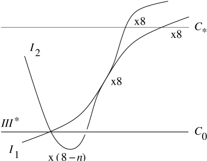
Figure 3: ${\mathbb{F}_{n,2}}$ with perturbative gauge group $E_{7}$ and instantons with $\mathbb{Z}_{2}$ holonomy

To reconstruct the complete degenerated threefold, we have to glue the bases of the two threefold $X_{1}$ and $X_{2}$ together along $C_{*}$. To be consistent, the singular fibres over $C_{*}$ must be the same on each of $X_{1}$ and $X_{2}$. Recall that for the $\operatorname{\mathit{SO}}(16)$ factor $X_{1}$ had a single curve of $\operatorname{\mathit{I}}_{1}$ fibres intersecting $C_{*}$ eight times and eight curves of $\operatorname{\mathit{I}}_{2}$ fibres intersecting $C_{*}$ once. These intersections must then match those on the $\operatorname{\mathit{SU}}(2)\times E_{7}$ factor $X_{2}$ which also had a single curve of $\operatorname{\mathit{I}}_{1}$ fibres intersecting $C_{*}$ eight times together with a single curve of $\operatorname{\mathit{I}}_{2}$ fibres intersecting $C_{*}$ eight times. The full degenerated threefold is shown in Figure 4. Note that $C_{*}$ has eight $\operatorname{\mathit{I}}_{1}$ fibres and eight $\operatorname{\mathit{I}}_{2}$ fibres and so is indeed a K3 surface, reproducing the heterotic K3 surface $Y$. The $\operatorname{\mathit{I}}_{2}$ fibres give eight $A_{1}$ singularities. Clearly, although locally near the orbifold points we have the same geometry and perturbative bundles as the $T^{4}/\mathbb{Z}_{2}$ model, globally we have a different limit of the K3 manifold since we have only eight fixed points and not sixteen.

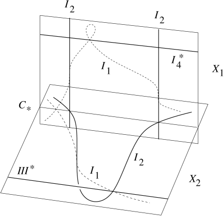
Figure 4: The full degenerate space $\mathbb{F}_{n,1}\vee\mathbb{F}_{n,2}$

3.3 M-theory limit

Having constructed the F-theory model we can now take the M-theory limit to compare with the rules given in [6, 7]. Recall that the stable degeneration corresponds to shrinking one of the $S^{1}$ cycles in the $\mathbb{P}^{1}$ fibre of $\mathbb{F}_{n}$ to a point, to form a pair of intersecting $\mathbb{P}^{1}$ curves. Following [12] (see also [21]), taking the M-theory limit requires shrinking a whole family of $S^{1}$ cycles to points, so that the sphere $\mathbb{P}^{1}$ becomes a one-dimensional interval. This reduces the threefold $X$ to a five-dimensional manifold and which can be viewed as the M-theory compact space $S^{1}/\mathbb{Z}_{2}\times Y$.

The five-dimensional manifold can be still represented by the diagram, Figure 4, though now the $\mathbb{P}^{1}$ fibres of $\mathbb{F}_{n,1}$ and $\mathbb{F}_{n,2}$ must be viewed as forming a single $S^{1}/\mathbb{Z}_{2}$ interval bounded by the $C_{0}$ sections which represent the fixed ten-planes. The manifold $Y$ is fixed by the K3 surface over $C_{*}$. The $A_{1}$ orbifold singularities are described by the curve of $\operatorname{\mathit{I}}_{2}$ fibres. Note that on $X_{1}$ these intersect $C_{0}$ transversally and the space looks something like a product $Y\times S^{1}/\mathbb{Z}_{2}$, with the lines of $\operatorname{\mathit{I}}_{2}$ fibres describing the fixed seven-planes. However, on $X_{2}$, the curve of $\operatorname{\mathit{I}}_{2}$ fibres has a component parallel to the $C_{0}$ and so the fixed-seven planes are distorting. From this it is clear that the geometry of the full M-theory space is not simply a product. This supports the similar conclusion reached above arguing directly from M-theory.

What gauge and matter fields do we find present in the M-theory limit? First consider the gauge groups. We have $\operatorname{\mathit{SO}}(16)$ and $E_{7}$ factors from singular fibres over the $C_{0}$ sections for $X_{1}$ and $X_{2}$ respectively. On $X_{1}$ it appears we have eight distinct $\operatorname{\mathit{SU}}(2)$ factors, one for each $A_{1}$ singularity on $Y$. These correspond to the fixed seven-planes of the M-theory $T^{4}/\mathbb{Z}_{2}\times S^{1}/\mathbb{Z}_{2}$ manifold. However, from the intersection over $C_{*}$, we see that each of these connects to the single curve of $\operatorname{\mathit{SU}}(2)$ singularities on $X_{2}$. Thus over the whole (degenerate) space $X$, there is only a single curve of $\operatorname{\mathit{SU}}(2)$ singularities, which is the source of the $\operatorname{\mathit{SU}}(2)^{*}$ factor in $\operatorname{\mathit{SO}}(16)\times[\operatorname{\mathit{SU}}(2)^{*}\times E_{7}]$. In other words, we see directly that the $\operatorname{\mathit{SU}}(2)$ factors on the the fixed seven-planes must be identified with the perturbative $\operatorname{\mathit{SU}}(2)$, justifying the arguments in [6, 7].

The matter appears as follows. First, there are the usual perturbative hypermultiplets $(\mathbf{128},\mathbf{1},\mathbf{1})$ and $(\mathbf{1},\mathbf{2},\mathbf{56})$ in $\operatorname{\mathit{SO}}(16)\times[\operatorname{\mathit{SU}}(2)\times E_{7}]$. In F-theory these correspond to the possibility of blowing-up the singularities and Higgsing the preserved gauge group [19]. However, in addition, we get extra matter when different parts of the discriminant curve intersect [19, 22, 23, 24]. In particular, the intersection of the curve of $\operatorname{\mathit{I}}_{2}$ fibres and the $\operatorname{\mathit{IV}}^{*}$ fibres over $C_{0}$ in $X_{1}$, lead to sixteen half hypermultiplets in fundamental representations $\frac{1}{2}(\mathbf{16},\mathbf{2},\mathbf{1})$. This is precisely the twisted matter of the perturbative heterotic string. It is easy to see how this can be charged under gauge groups coming from both of the fixed ten-planes, because, in the distorted M-theory geometry, the $\operatorname{\mathit{SU}}(2)$ gauge group is seen to “stretch” across the $S^{1}/\mathbb{Z}_{2}$ orbifold to intersect the $\operatorname{\mathit{SO}}(16)$ fixed plane. Again, we find an F-theory justification for the arguments in [6, 7] as to how the twisted matter appears.

Recall that, while locally the F-theory model gave a heterotic K3 surface with $A_{1}$ singularities, globally the surface was not $T^{4}/\mathbb{Z}_{2}$. This is reflected by the fact that there were only eight $A_{1}$ singularities and, in addition, a curve of $\operatorname{\mathit{I}}_{1}$ fibres on $X$. On $X_{1}$ this curve has $(4-n)$ double intersections with $C_{0}$. Following [10] these are interpreted as ordinary pointlike instantons on $Y$. As a result, there are an additional $(4-n)$ tensor multiplets in the spectrum, parametrising the “Coulomb” branch describing the motion of the instantons into the $S^{1}/\mathbb{Z}_{2}$ bulk as M5-branes [25, 26]. Similarly, there are $(8-n)$ mutual intersections of the $\operatorname{\mathit{I}}_{1}$, $\operatorname{\mathit{I}}_{2}$ and $C_{0}$ curves in $X_{2}$ leading to a further $(8-n)$ pointlike-instanton tensor multiplets. Note that this provides a check that the instanton charge of the fractional instantons at the $A_{1}$ singularities in the model is as expected. Recall that each $\mathbb{F}_{n}$ plane carries a total instanton number of $12-n$ [19, 10]. Each ordinary pointlike instanton carries charge one. Thus the eight fractional instantons on $X_{1}$ must also each carry charge one. On $X_{2}$ however, each of the eight fractional instantons must carry charge $1/2$. This matches exactly the expected charges for $\operatorname{\mathit{SO}}(16)$ and $\operatorname{\mathit{SU}}(2)\times E_{7}$ perturbative bundles discussed above.

Let us end this section by briefly discussing how the F-theory model should be modified so that one realises the exact global dual of the $T^{4}/\mathbb{Z}_{2}$ compactification rather than simply the local behaviour near the $A_{1}$ singularities. The essential point is that $T^{4}/\mathbb{Z}_{2}$ cannot be realized directly as a conventional Weierstrass model of the form (3.1) with $\operatorname{\mathit{I}}_{2}$ fibres. Instead one takes a model with four $D_{4}$ singularities, giving gauge group $\operatorname{\mathit{SO}}(8)^{4}$ and then blows up one cycle in each fiber to Higgs the $\operatorname{\mathit{SO}}(8)$ group to $\operatorname{\mathit{SU}}(2)^{4}$, giving four $A_{1}$ singularities per fibre. To realise the F-theory dual, we fix $n=4$ on the $E_{7}$ half-plane and $n=-4$ on the $\operatorname{\mathit{SO}}(16)$ plane. To reproduce the four $D_{4}$ singularities on $C_{*}$ we have to restrict to the case where the eight $\operatorname{\mathit{I}}_{1}$ fibres and eight $\operatorname{\mathit{I}}_{2}$ fibres on $C_{*}$ come together in four sets of two $\operatorname{\mathit{I}}_{1}$ and two $\operatorname{\mathit{I}}_{2}$. This restricts the form of the discriminant curves (3.6) and (3.9). In particular, on the $\operatorname{\mathit{SO}}(16)$ plane the function $h$ in (3.5) must factor as $h=f_{1}^{2}f_{2}^{2}f_{3}^{2}f_{4}^{2}$ to give four curves of $\operatorname{\mathit{I}}_{0}^{*}$ fibres with $D_{4}$ singularities.

4 Other cases and discussion

Let us end by mentioning how this analysis can be extended to other orbifold compactifications, starting with other examples on $T^{4}/\mathbb{Z}_{2}$. The F-theory analysis justified local rules for gauge groups and matter at the $A_{1}$ singularities. In particular, for a charge $1/2$ fractional instanton leaving the gauge group $\operatorname{\mathit{SU}}(2)\times E_{7}$, we saw that there was an $\operatorname{\mathit{SU}}(2)$ gauge group on the fixed seven-plane which is identified with the perturbative $\operatorname{\mathit{SU}}(2)$. No additional matter appeared at the intersection of the seven- and the ten-plane. For a unit charge fractional instanton leaving gauge group $\operatorname{\mathit{SO}}(16)$, there was again an $\operatorname{\mathit{SU}}(2)$ gauge group on the seven-plane, and now additional hypermultiplets at the intersection transforming as $\frac{1}{2}(\mathbf{16},\mathbf{2})$ under $\operatorname{\mathit{SO}}(16)\times\operatorname{\mathit{SU}}(2)$.

In [6] further rules have been developed for other types of instanton at $A_{1}$ singularities. In particular, one very obvious case to consider is the conventional perturbative heterotic background with the standard embedding. This has charge $3/2$ fractional instantons on one ten-plane and none on the other, leaving a gauge group $E_{8}\times[\operatorname{\mathit{SU}}(2)\times E_{7}]$. Notably, unlike the example above, this background has no perturbative states charged under gauge groups from different ten-planes. In turns out that, as shown by Aspinwall and Donagi [27] the F-theory dual of the standard embedding is particularly subtle. In particular, it is crucial that one considers the role of the Ramond–Ramond (RR) fields in order to distinguish it from other duals. The effect is that for non-zero RR backgrounds less gauge symmetry is preserved than might immediately appear from the geometry. Nonetheless, one would expect that a similar analysis of the M-theory limit as above is possible. A further generalization in [6, 7], are models with $E_{8}\times[\operatorname{\mathit{SU}}(2)\times E_{7}]$ or $E_{8}\times E_{8}$ perturbative symmetry and additional $U(1)$ non-perturbative factors. In general, $U(1)$ factors are hard to identify in F-theory models, though are still encoded in the geometry as discussed for instance in [28].

One model that can be easily analysed is that with $\operatorname{\mathit{SO}}(8)^{8}$ gauge group considered in [4]. This was argued to be dual to F-theory on $T^{6}/(\mathbb{Z}_{2}\times\mathbb{Z}_{2})$, with a base manifold $T^{2}/\mathbb{Z}_{2}\times T^{2}/\mathbb{Z}_{2}$ which is a singular limit of $\mathbb{F}_{0}=\mathbb{P}^{1}\times\mathbb{P}^{1}$. Following [11], in this case we expect that the heterotic background has $\mathbb{Z}_{2}\times\mathbb{Z}_{2}$ fractional instantons at the $A_{1}$ singularities, preserving a perturbative $\operatorname{\mathit{SO}}(8)^{2}$ for each $E_{8}$ factor. The Weierstrass model then takes the form

$$a =\frac{1}{3}(b_{2}c_{2}-b_{2}^{2}-c_{2}^{2}),$$ (4.1)

$$b =-\frac{1}{27}(b_{2}+c_{2})(b_{2}-2c_{2})(2b_{2}-c_{2}),$$

$$\delta =-b_{2}^{2}c_{2}^{2}(b_{2}-c_{2})^{2},$$

where $b_{2}$ and $c_{2}$ are sections of $\mathcal{L}^{2}$. Taking the stable degeneration, one gets the correct gauge group by taking

$$b_{2}=c_{1}c_{2}f_{1}\dots f_{4}$$ (4.2)

one each of $\mathbb{F}_{0,1}$ and $\mathbb{F}_{0,2}$. The functions $c_{1}$ and $c_{2}$ define two different sections in the divisor class of the first $\mathbb{P}^{1}$ factor in $\mathbb{F}_{0}=\mathbb{P}^{1}\times\mathbb{P}^{1}$, and $f_{1}$ to $f_{4}$ give four different sections in the class of the second factor. The two $c_{1}=0$ and $c_{2}=0$ curves intersect the four $f_{i}=0$ curves transversally. From the discriminant curve, each function defines a curve of $\operatorname{\mathit{I}}_{0}^{*}$ fibres giving an $\operatorname{\mathit{SO}}(8)$ factor. Gluing $X_{1}$ and $X_{2}$ together, we must identify the two sets of $f_{i}=0$ curves and so the full gauge group becomes $\operatorname{\mathit{SO}}(8)^{8}$. Four $\operatorname{\mathit{SO}}(8)$ factors are perturbative and four non-perturbative. As pointed out in [4], there is a symmetry exchanging perturbative and non-perturbative factors, essentially by exchanging the role of the two $\mathbb{P}^{1}$ factors in each $\mathbb{F}_{0}$. Note that as stands this is not quite the required model. As in the discussion at the end of the last section, the K3 manifold over the $C_{*}$ intersection is not $T^{4}/\mathbb{Z}_{2}$ but a more singular space with four $D_{4}$ singularities. To obtain $T^{4}/\mathbb{Z}_{2}$ we must blow up one curve in each singular fibre, thus Higgsing $\operatorname{\mathit{SO}}(8)$ to $\operatorname{\mathit{SU}}(2)^{4}$. In general this blows up the corresponding fibres in the $f_{i}=0$ curves so the full symmetry is actually $\operatorname{\mathit{SU}}(2)^{16}\times\operatorname{\mathit{SO}}(8)^{4}$. To preserve the symmetry between perturbative and non-perturbative groups, one would also blow up one cycle in the fibres above each of the $c_{1}=0$ and $c_{2}=0$ sections so that the final gauge symmetry becomes $(SU(2))^{32}$.

The other obvious class of generalisations is to other K3 orbifolds. Again [6, 7] give rules for instantons at other types of singularity. The most straightforward generalisation is the $\mathbb{Z}_{3}$ version of the $\mathbb{Z}_{2}$ model considered above. The orbifold $T^{4}/\mathbb{Z}_{3}$ has nine $A_{2}$ singularities and there are two types of $\mathbb{Z}_{3}$-holonomy bundles, preserving either $\operatorname{\mathit{SU}}(9)$ or $\operatorname{\mathit{SU}}(3)\times E_{6}$. The perturbative model with both groups $\operatorname{\mathit{SU}}(9)\times[\operatorname{\mathit{SU}}(3)\times E_{6}]$ is the analogue of the $\mathbb{Z}_{2}$ example considered above. This example was explicitly worked out in [11]. One finds a Weierstrass model with

$$a =a_{1}\left(\frac{1}{2}a_{3}-\frac{1}{48}a_{1}^{3}\right),$$ (4.3)

$$b =\frac{1}{4}a_{3}^{2}+\frac{1}{864}a_{1}^{6}-\frac{1}{24}a_{1}^{3}a_{3},$$

$$\delta =\frac{1}{16}a_{3}^{3}(27a_{3}-a_{1}^{3}).$$

where $a_{i}$ is a section of $\mathcal{L}^{i}$. In the stable degeneration limit, on the $\operatorname{\mathit{SU}}(9)$ threefold one takes

$$a_{1}=g,\qquad a_{3}=c_{0}^{3}f_{1}\dots f_{6},$$ (4.4)

where $c_{0}$ vanishes on $C_{0}$, the $f_{i}$ vanish on distinct fibres and $g=0$ is in the class $C_{0}+2f$. This gives a curve of $\operatorname{\mathit{I}}_{9}$ fibres with $\operatorname{\mathit{SU}}(9)$ on $C_{0}$, six curves $f_{i}=0$ of $\operatorname{\mathit{I}}_{3}$ fibres with $\operatorname{\mathit{SU}}(3)$ and a single curve of $\operatorname{\mathit{I}}_{1}$ fibres. On the $\operatorname{\mathit{SU}}(3)\times E_{6}$ threefold one takes

$$a_{1}=c_{0}f_{1}f_{2},\qquad a_{3}=c_{0}^{2}h,$$ (4.5)

where the $f_{i}$ vanish on distinct fibres and $h=0$ is in the class $C_{0}+6f$. This gives a curve of $\operatorname{\mathit{IV}}^{*}$ fibres with $E_{6}$ on $C_{0}$, a single curve of $\operatorname{\mathit{I}}_{3}$ fibres with $\operatorname{\mathit{SU}}(3)$ on $h=0$ and a single curve of $\operatorname{\mathit{I}}_{1}$ fibres. Again, gluing $X_{1}$ and $X_{2}$ means that the $\operatorname{\mathit{SU}}(3)$ factors are identified as a single curve so the final gauge symmetry becomes $\operatorname{\mathit{SU}}(9)\times[\operatorname{\mathit{SU}}(3)^{*}\times E_{6}]$ in direct analogy with the $\mathbb{Z}_{2}$ example. There are related models with $\mathbb{Z}_{4}$ and $\mathbb{Z}_{6}$ symmetry which it should be possible to analyse in an analogous fashion.

In summary, we have shown that known results for the F-theory duals of different Hořava–Witten orbifold compactifications provide a good explanation of some of the more counter-intuitive rules implied by anomaly cancellation in the M-theory model. In particular, it becomes clear why in some cases gauge groups on the fixed seven-planes should be identified with perturbative gauge groups on the fixed ten-planes. Also, this provides additional evidence that the actual M-theory geometry is not simply a product. One interesting extension would be to explore this geometry further directly in the M-theory model. It also appears to be possible to extend the analysis to various other orbifold models and perhaps use this approach to analyse M-theory orbifold compactifications to four dimensions.

Acknowledgements

Both authors are supported in part by PPARC through the grant SPG $\#$613. DW also thanks the Royal Society for support and the Isaac Newton Institute at the University of Cambridge for hospitality during the completion of this manuscript. The work of MM was also supported by the University of Halle and a Marie Curie Postgraduate Fellowship by the EU. MM thanks the Physics Department of Queen Mary College, University of London, for hospitality while the work presented here was done.

References

-
[1]
P. Horava, E. Witten, “Heterotic And Type I String Dynamics From
Eleven Dimensions”, Nucl. Phys. B460 506 (1996),
hep-th/9510209;
P. Horava, E. Witten, “ Eleven-Dimensional Supergravity On A Manifold With Boundary ”, Nucl. Phys. B475 94 (1996), hep-th/9603142. - [2] E. Witten, “Five-Branes and M-Theory on an Orbifold”, Nucl. Phys. B463 383 (1996)), hep-th/9512219;
- [3] K. Dasgupta and S. Mukhi, “Orbifolds of M-theory,” Nucl. Phys. B 465, 399 (1996), hep-th/9512196.
- [4] R. Gopakumar, C. Mukhi, “Orbifold and Orientifold Compactification of F-Theory and M-Theory to Six and Four Dimensions”, Nucl. Phys. B479 260 (1996), hep-th/9607057.
- [5] K. A. Meissner and M. Olechowski, “Anomaly cancellation in M-theory on orbifolds,” Nucl. Phys. B 590, 161 (2000), hep-th/0003233.
-
[6]
M. Faux, D. Lüst, B.A. Ovrut, “Intersection Orbifold Planes and
Local Anomaly Cancellation in M-Theory”, Nucl. Phys. B554 (1999), hep-th/9903028;
M. Faux, D. Lüst, B.A. Ovrut, “Local Anomaly Cancellation, M-Theory Orbifolds and Phase-Transitions”, Nucl. Phys. B589 (2000), hep-th/0005251;
M. Faux, D. Lüst, B.A. Ovrut, “An M-Theory Perspective on Heterotic Orbifold Compactifications”, hep-th/0010087;
M. Faux, D. Lüst, B.A. Ovrut, “Twisted Sectors and Chern-Simons Terms in M-Theory Orbifolds”, hep-th/0011031. - [7] V. Kaplunovsky, J. Sonnenschein, S. Theisen, S. Yankielowicz, “On The Duality Between Perturbative Heterotic Orbifolds And M-Theory On ”, Nucl. Phys. B590 (2000), hep-th/9912144.
- [8] C. Doran, M. Faux, B.A. Ovrut, “ Four-Dimensional Super Yang-Mills Theory from an M-Theory Orbifold”, hep-th/0108078.
- [9] E. Gorbatov, V. Kaplunovsky, J. Sonnenschein, S. Theisen, S. Yankielowicz, “On Heterotic Orbifolds, M-Theory and Type I’ Brane Engineering”, hep-th/0108135.
- [10] P.S. Aspinwall, D.R. Morrison, “Point-like Instantons On Orbifolds ”, Nucl. Phys. B503 (1997), hep-th/9705104.
- [11] P.S. Aspinwall, D.R. Morrison, “ Non-Simply Connected Gauge Groups and Rational Points on Elliptic Curves ”, JHEP 9807 (1998) 12, hep-th/9805206.
- [12] P.S. Aspinwall, “M-Theory Versus F-theory Picutures of the Heterotic String”, Adv. Theor. Math. Phys. 1 (1998) 127, hep-th/9707014.
-
[13]
P. Candelas and A. Font,
“Duality between the webs of heterotic and type II vacua,”
Nucl. Phys. B 511 (1998) 295, hep-th/9603170;
P. Candelas, E. Perevalov and G. Rajesh, “F-theory duals of non-perturbative heterotic vacua in six dimensions,” Nucl. Phys. B 502, 613 (1997), hep-th/9606133;
P. Candelas, E. Perevalov and G. Rajesh, “Matter from toric geometry,” Nucl. Phys. B 519, 225 (1998), hep-th/9707049. - [14] M. Berkooz, R. G. Leigh, J. Polchinski, J. H. Schwarz, N. Seiberg, E. Witten, “Anomalies, Dualities, and Topology of Superstring Vacua”, Nucl. Phys. B475 115 (1996), hep-th/9605184.
- [15] M. A. Walton, “The Heterotic String On The Simplest Calabi–Yau Manifold And Its Orbifold Limits,” Phys. Rev. D 37, 377 (1988).
- [16] J. Erler, “Anomaly Cancellation in Six Dimensions”, J.Math. Phys. 35 1819 (1994), hep-th/9304104.
- [17] A. Lukas, B. A. Ovrut and D. Waldram, “On the four-dimensional effective action of strongly coupled heterotic string theory,” Nucl. Phys. B 532 (1998) 43, hep-th/9710208.
- [18] E. Witten, “Strong Coupling Expansion Of Calabi-Yau Compactification,” Nucl. Phys. B 471, 135 (1996), hep-th/9602070.
-
[19]
D.R. Morrison, C. Vafa, “Compactification of F-Theory on
Calabi-Yau Threefolds-I”, Nucl. Phys. B473 (1996),
hep-th/9602114;
D.R. Morrison, C. Vafa, “Compactification of F-Theory on Calabi-Yau Threefolds-II”, Nucl. Phys. B476 (1996), hep-th/9603161. - [20] R. Friedman, J. Morgan, E. Witten, “ Vector Bundles and F-Theory”, Commun. Math. Phys. 187 (1999), hep-th/9701162.
- [21] P.S. Aspinwall, D.R. Morrison, “ U-Duality and Integral Structures ”, Phys. Lett. 355B (1995), hep-th/9505025..
- [22] M. Bershadsky, C. Vafa and V. Sadov, “D-Strings on D-Manifolds,” Nucl. Phys. B 463, 398 (1996), hep-th/9510225.
- [23] S. Katz and C. Vafa, “Matter from geometry,” Nucl. Phys. B 497, 146 (1997), hep-th/9606086.
- [24] P. S. Aspinwall, S. Katz and D. R. Morrison, “Lie groups, Calabi-Yau threefolds, and F-theory,” Adv. Theor. Math. Phys. 4, 95 (2000), hep-th/0002012.
- [25] O. J. Ganor and A. Hanany, “Small Instantons and Tensionless Non-critical Strings,” Nucl. Phys. B 474 122 (1996), hep-th/9602120.
- [26] N. Seiberg, E. Witten, “Comments on String Dynamics in Six Dimensions”, Nucl. Phys. B471 121 (1996), hep-th/9603003.
- [27] P. Aspinwall, R. Donagi, “The Heterotic String, the Tangent Bundle, and Derived Categories”, Adv. Theor. Math. Phys. 2 1041 (1998), hep-th/9806094.
- [28] Z. Guralnik, “String Junctions and Non-Simply Connected Gauge Groups”, JHEP 0107 2 (2001), hep-th/0102031.