TPI-MINN-02/6

UMN-TH-2046/02

Duality and Self-Duality (Energy Reflection Symmetry) of Quasi-Exactly Solvable Periodic Potentials

Gerald V. Dunne

Department of Physics, University of Connecticut
2152 Hillside Road, Storrs, CT 06269

M. Shifman

Theoretical Physics Institute, University of Minnesota,
116 Church St. S.E., Minneapolis, MN 55455

Abstract

A class of spectral problems with a hidden Lie-algebraic structure is considered. We define a duality transformation which maps the spectrum of one quasi-exactly solvable (QES) periodic potential to that of another QES periodic potential. The self-dual point of this transformation corresponds to the energy-reflection symmetry found previously for certain QES systems. The duality transformation interchanges bands at the bottom (top) of the spectrum of one potential with gaps at the top (bottom) of the spectrum of the other, dual, potential. Thus, the duality transformation provides an exact mapping between the weak coupling (perturbative) and semiclassical (nonperturbative) sectors.

1 Introduction

Quasi-exactly solvable (QES) systems are those for which some finite portion of the energy spectrum can be found exactly using algebraic means [1, 2, 3, 4, 5]. A positive integer parameter $J$ characterizes the ‘size’ of this exact portion of the spectrum. This integer $J$ has both an algebraic significance, related to the dimension of a representation, and a geometrical significance, the genus of a Riemann surface associated with the spectrum. In [6], the large $J$ limit was identified as a semiclassical limit useful for studying the top of the quasi-exact spectrum. It was found that remarkable factorizations reduce the semiclassical calculation to simple integrals, leading to a straightforward asymptotic series representation for the highest QES energy eigenvalue. The notion of energy-reflection (ER) symmetry was introduced and analyzed in [7]: for certain QES systems the QES portion of the spectrum is symmetric under the energy reflection $E\to-E$. This means that for a system with ER symmetry, there is a precise connection between the top of the QES spectrum and the bottom of the spectrum. Coupled with the semiclassical large $J$ limit, the ER symmetry relates semiclassical (nonperturbative) methods with perturbative methods [7]. In this present paper, we show that for a class of periodic QES potentials the ER symmetry is in fact the fixed point (self-dual point) of a more general duality transformation. The duality transformation we consider is analogous to, but importantly different from, a similar transformation suggested in Ref. [8] relating different QES potentials.

For periodic potentials, usually, the Lie-algebraic QES sector consists of band boundaries which correspond either to periodic or antiperiodic boundary conditions . Thus, only one boundary of each band is algebraic. However, for the elliptic periodic potentials to be considered below, both boundaries are algebraically calculable. For given $J$, there are $2J+1$ energy eigenvalues in the algebraic sector; there are $J+1$ allowed bands, with the highest band being open (it stretches up to $E=\infty$). The $2J+1$ algebraic energy levels give all band edges, so that in the problem at hand all band edges are algebraically calculable. This fact is well-known in the literature. In this paper the main emphasis is on physical aspects which have not been investigated so far. When the parameter $J$ becomes large, the theory becomes weakly coupled at the bottom of the spectrum and semiclassical at the top. We develop this idea — using $1/J$ as an expansion parameter — in the application to the elliptic periodic potentials. We show that the duality between weak coupling and semiclassical expansions applies not just to the asymptotic series for the locations of the bands and gaps, but also to the exponentially small widths of bands and gaps. We observe that the $2J+1$-level algebraic sector splits into four completely disconnected algebraic subsectors. Therefore, instead of diagonalizing a $(2J+1)\times(2J+1)$ matrix, it is sufficient to diagonalize four matrices which are roughly four times smaller in their linear sizes. In addition to the eigenvalues, we determine, purely algebraically, the eigenfunctions corresponding to the band edges. For even $J$ there are $J+1$ periodic eigenfunctions and $J$ antiperiodic ones. For odd $J$ there are $J$ periodic eigenfunctions and $J+1$ antiperiodic ones.

In Sect. 2 we define our duality and self-duality transformation, and review some basic facts about the periodic Lamé equation. The duality transformation has both an algebraic and geometric interpretation. We show how the duality transformation extends the algebraic ER symmetry formalism introduced in [7]. Section 3 is devoted to a detailed consideration of four distinct $sl(2)$-based algebraizations relevant to the algebraic determination of the band edges and the corresponding wave functions. We explain why the cases of even and odd $J$ must be treated separately and how periodic and antiperiodic wave functions emerge. The periodicity versus antiperiodicity is due to properties of the quasiphases in these two cases. In Sect. 4 we study several explicit examples in detail. Section 5 is devoted to an analysis of the self-dual case. In Sect. 6 we describe the duality relation between perturbative and nonperturbative approximation techniques, as applied to the computation of both the locations and widths of bands and gaps. Finally, Sect. 7 contains a summary and some comments regarding further generalizations.

2 Duality and self-duality in Lamé model

In this section we introduce the notions of duality and self-duality for the following one-dimensional quasi-exactly solvable (QES) Lamé equation:

$$\left\{-\frac{d^{2}}{d\phi^{2}}+J(J+1)\,\nu\,{\rm sn}^{2}(\phi|\nu)-\frac{1}{2}J(J+1)\right\}\Psi(\phi)=E\,\Psi(\phi)\,.$$ (1)

Here ${\rm sn}(\phi|\nu)$ is the doubly-periodic Jacobi elliptic function [12, 13], the coordinate $\phi\in R^{1}$, and $E$ denotes the energy eigenvalue. The real elliptic parameter $\nu$ lies in the range $0\leq\nu\leq 1$. The potential in (1) has period $2K(\nu)$, where

$$K(\nu)=\int_{0}^{\pi/2}\frac{d\theta}{\sqrt{1-\nu\sin^{2}\theta}}$$ (2)

is the elliptic quarter period. Note that the parameter $\nu$ controls the period of the potential, as well as its strength. As $\nu\to 1$, the period $2K(\nu)$ diverges logarithmically, $2K(\nu)\sim\ln\,(\frac{16}{1-\nu})$, while as $\nu\to 0$, the period tends to a nonzero constant: $2K(\nu)\to\pi$. In the Lamé equation (1), the parameter $J$ is a positive integer (for non-integer $J$, the problem is not QES). This parameter $J$ controls the depth of the wells of the potential; the significance of the constant subtraction $-\frac{1}{2}J(J+1)$ will become clear below. As an illustration, we have plotted in Fig. 1 the potential energy in the Schrödinger equation (1) for two values of $\nu$, namely, $\nu=0.95$ and $\nu=0.05$.

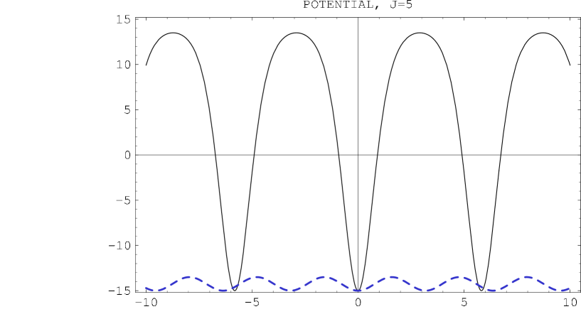
Figure 1: The potential energy in the Schrödinger equation (1) as a function of $\phi$. The solid curve corresponds to elliptic parameter $\nu=0.95$, for which the period is $2K(0.95)\approx 5.82$. The dashed curve corresponds to $\nu=0.05$, for which the period is $2K(0.05)\approx 3.18$. In each case, $J=5$. Note how different the two potentials are; and yet, their spectra are related by the duality transformation (5).

It is a classic result that the Lamé equation (1) has bounded solutions $\Psi(\phi)$ with an energy spectrum consisting of exactly $J$ bands, plus a continuum band [12]. It is the simplest example of a “finite-gap” [14, 15] model , there being just a finite number, $J$, of “gaps”, or “excluded bands” in the spectrum. This should be contrasted with the fact that a generic periodic potential has an infinite sequence of gaps in its spectrum [16]. We label the band edge energies by $E_{l}$, with $l=1,2,\dots,(2J+1)$. Thus, the energy regions, $E_{2l-1}\leq E\leq E_{2l}$, and $E\geq E_{2l+1}$, are the allowed bands (“bands” for short), while the regions, $E_{2l}<E<E_{2l+1}$, and $E<E_{1}$, are the exclusion bands (“gaps” for short). The wave functions $\Psi(\phi)$ at the band edges are either periodic or antiperiodic functions, with period $2K(\nu)$, while within the bands the wave functions are quasi-periodic Bloch functions, which can be expressed in terms of theta functions [12].

Another important classic result [17, 18, 19] concerning the Lamé model (1) is that the band edge energies $E_{l}$, for $l=1,\dots,2J+1$, are simply the eigenvalues of the $(2J+1)\times(2J+1)$ matrix

$$H=J_{x}^{2}+\nu J_{y}^{2}-\frac{1}{2}J(J+1)\,{\bf I}$$ (3)

where $J_{x}$ and $J_{y}$ are $su(2)$ generators in a spin $J$ representation and ${\bf I}$ is the unit matrix. Thus the Lamé band edge spectrum is algebraic, requiring only the finding of the eigenvalues of the finite dimensional matrix $H$ in (3). When $\nu=0\,\,{\rm or}\,\,1$, it is straightforward to write down the eigenvalues of $H$. But for $0<\nu<1$, the matrix $J_{x}^{2}+\nu J_{y}^{2}$ cannot be simply related to the $su(2)$ Casimir, $\vec{J}^{2}$, and so the eigenvalues of $H$ are, in fact, nontrivial functions of $\nu$. For example, for $J=1$ and $J=2$, the eigenvalues of $H$ are:

$$J=1\quad:\quad E_{1} = -1+\nu\,,$$

$$E_{2} = 0\,,$$

$$E_{3} = \nu\,;$$

$$J=2\quad:\quad E_{1} = -1+2\,\nu-2\,{\sqrt{1-\nu+\nu^{2}}}\,,$$

$$E_{2} = -2+\nu\,,$$

$$E_{3} = -2+4\,\nu\,,$$

$$E_{4} = 1+\nu\,,$$

$$E_{5} = -1+2\,\nu+2\,{\sqrt{1-\nu+\nu^{2}}}\,.$$ (4)

The band (gap) structure in the second case, $J=2$, is presented in Fig. 2.

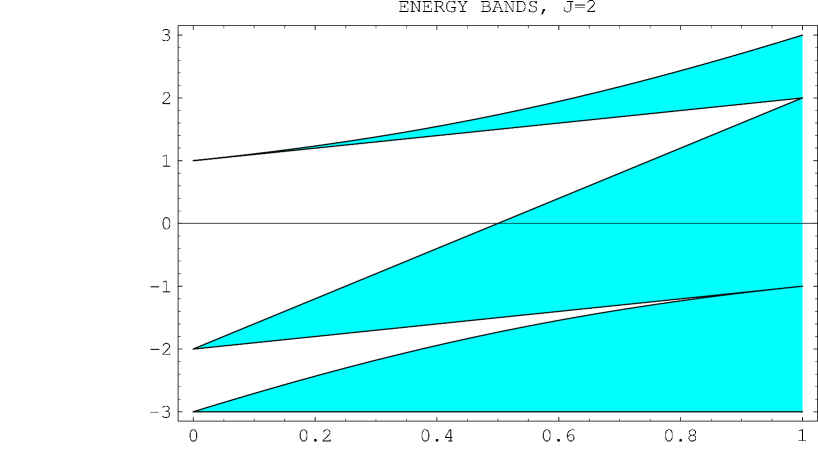
Figure 2: The energy bands for the Lamé system (1), as a function of $\nu$. The plot given is for $J=2$. The first (the lowest) allowed band (unshaded) is of the p-ap type, while the second one of the ap-p type, see text.

The shaded areas on this plot (and other similar plots in Figs. 4, 5 and 6) are the forbidden bands (gaps), while the unshaded areas are the allowed bands. The allowed bands can be of two types: p-ap and ap-p. In the allowed bands of the first type the lower boundary of the band is determined by a periodic wave function, while the upper boundary by an anti-periodic one. In the allowed bands of the ap-p type, the band edge structure is reversed: the lower boundary corresponds to an anti-periodic wave function. The last allowed band has no upper boundary — it stretches up to infinitely high energies.

In [20], the algebraic form (3) of the Lamé system was exploited to provide a precise analytic test of the instanton approximation, as is discussed further in Sect. 6.

In this paper we study a special duality of the spectrum of the Lamé system (1), which can be stated succinctly as:

$$E[\nu]=-E[1-\nu]$$ (5)

where $E[\nu]$ denotes the spectrum for the potential with elliptic parameter $\nu$. That is, the spectrum of the Lamé system (1), with elliptic parameter $\nu$, is the energy reflection of the spectrum of the Lamé system with the dual elliptic parameter $1-\nu$. In particular, for the band edge energies, $E_{l}$, which are the eigenvalues of the finite dimensional matrix $H$ in (3), this means that (for $l=1,2,\dots,2J+1$)

$$E_{l}[\nu]=-E_{2J+2-l}\,[1-\nu]$$ (6)

This duality can be seen directly in the eigenvalues of the $J=1$ and $J=2$ examples in (4). The proof for the band edge energies is a trivial consequence of the algebraic realization (3), since

$$H[\nu] \equiv J_{x}^{2}+\nu J_{y}^{2}-\frac{1}{2}J(J+1)\,{\bf I}$$ (7)

$$= -\left[\left(J_{z}^{2}+(1-\nu)J_{y}^{2}\right)-\frac{1}{2}J(J+1)\,{\bf I}\right]\,.$$

Noting that $[J_{z}^{2}+(1-\nu)J_{y}^{2}]$ has the same eigenvalues as $[J_{x}^{2}+(1-\nu)J_{y}^{2}]$, the duality result (6) follows. It is instructive to see this duality in graphical form, by looking at Figs. 2, 4, 5 and 6, which show the band spectra, as a function of $\nu$, for various different values of $J$. In each case, the transformation $\nu\to 1-\nu$, together with the energy reflection $E\to-E$, interchanges the shaded regions (the gaps) with the unshaded regions (the bands).

The fixed point, $\nu=\frac{1}{2}$, is the “self-dual” point, where the system maps onto itself, and the energy spectrum has an energy reflection (ER) symmetry, as was studied in [7]. In Sects. 3 and 4 we discuss in detail how this Lamé model fits into the energy reflection symmetry classification of Shifman and Turbiner.

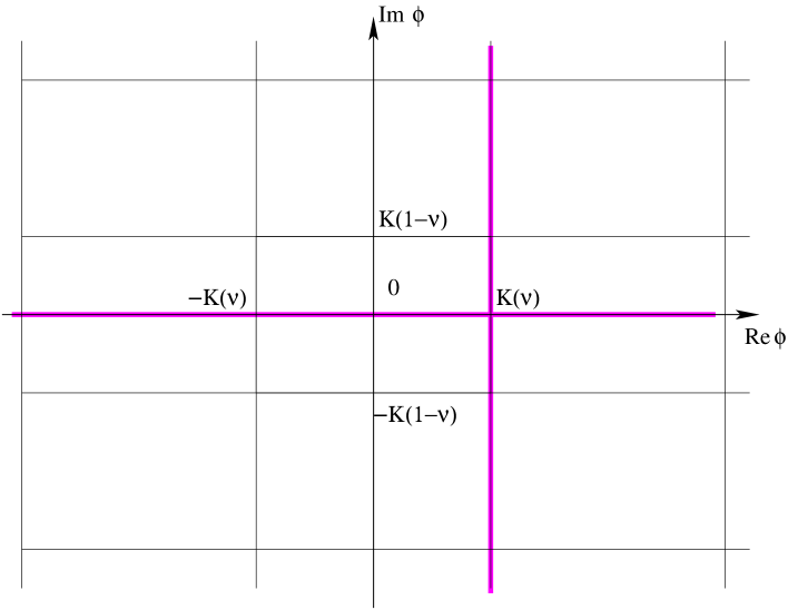
Figure 3: The period parallelogram for ${\rm sn}^{2}(\phi|\nu)$ is the rectangle with the sides $2K(\nu)$ and $2K^{\prime}(\nu)\equiv 2K(1-\nu)$. The original Lamé equation (1) is defined for real $\phi$, on the horizontal thick line. The dual Lamé equation is defined for $\phi$ on the vertical thick line. The parametric coordinate rotation is (8), and leads to the dual Lamé equation (10).

In fact, the duality relation (5) applies to the entire spectrum, not just the band edges (6). The easiest way to see this is to realize that the duality relation is a simple consequence of Jacobi’s imaginary transformation, applied to the Lamé equation (1). The original Lamé system (1) was defined for real coordinate $\phi$, but we can extend $\phi$ into the complex plane. The potential is doubly periodic, with real period $2K$ and imaginary period $2K^{\prime}\equiv 2K(1-\nu)$, as is shown in Fig. 3. Consider rotating the coordinate off the real axis by the transformation

$$\phi^{\prime}=i\left(\phi-K-i\,K^{\prime}\right)\,,$$ (8)

so that real $\phi^{\prime}$ can be considered as a parametric coordinate for $\phi$ running along a vertical line through the point $K$ (the vertical thick line in Fig. 3). Note that along this vertical line the potential ${\rm sn}^{2}(\phi|\nu)$ is again real. Moreover, using the properties of the Jacobi elliptic functions, [12, 13], we get

$$\nu\,{\rm sn}^{2}(K+iK^{\prime}-i\phi^{\prime}|\nu)=1-(1-\nu)\,{\rm sn}^{2}(\phi^{\prime}|1-\nu)\,.$$ (9)

The Lamé equation on the real axis maps to another, dual, Lamé equation on the vertical thick line (see Fig. 3). In other words, the change of variables (8) transforms the Lamé equation (1) into:

$$\left\{-\frac{d^{2}}{d\phi^{\prime 2}}+J(J+1)\,(1-\nu)\,{\rm sn}^{2}(\phi^{\prime}|1-\nu)-\frac{1}{2}J(J+1)\right\}\Psi(\phi^{\prime})=-E\,\Psi(\phi^{\prime})\,,$$ (10)

So solutions of the Lamé equation (1) are mapped to solutions of the dual equation (10), $\nu\to 1-\nu$, and with a sign reflected energy eigenvalue: $E\to-E$. Returning to the complex $\phi$ plane diagram in Fig. 3, the transformation (8) clearly interchanges the real and imaginary periods. In the self-dual case, $\nu=\frac{1}{2}$, these two periods are equal, so the periodic lattice shown in Fig. 3 is a square lattice. This is the so-called lemniscate case .

It is important to distinguish our duality transformation from another duality transformation considered in [8], for which the duality transformation was $\phi^{\prime}=i\,\phi$, which maps the real axis onto the imaginary axis. The Lamé potential is also real along the imaginary axis. However, along the imaginary axis there is a singularity at $\phi=i\,K^{\prime}$. The transformation $\phi^{\prime}=i\,\phi$ maps the original Lamé potential to a very different potential; so there is no notion of “self-duality” for this transformation.

To see why bands and gaps are interchanged under our duality transformation (8), we recall that the two independent solutions of the original Lamé equation (1) can be written as products of theta functions

$$\Psi_{\pm}(\phi)=\prod_{j=1}^{J}\left[\frac{\vartheta_{1}(\phi\pm\alpha_{j})}{\vartheta_{4}(\phi)}\,\exp\left(\mp\phi\,Z(\alpha_{j})\right)\right]$$ (11)

where the parameters $\alpha_{j}$, for $j=1,\dots,J$, satisfy a complicated set of $J$ nonlinear constraints together with the energy $E$, and $Z(\alpha)$ is the Jacobi zeta function [12]. Under the change of variables (8) these theta functions map into the same theta functions, but with dual elliptic parameter. However, they map from bounded to unbounded solutions (and vice versa), because of the “i” factor appearing in (8). Thus, the bands and gaps become interchanged. This interpretation of the duality transformation in terms of the Jacobi imaginary transformation will be important in Sect. 6 when we discuss WKB techniques.

Away from the self-dual point, $\nu=\frac{1}{2}$, the duality transformation relates the spectrum of one elliptic potential with the spectrum of a different elliptic potential. For example, the two potentials plotted in Fig. 1, for $\nu=0.95$ and $\nu=0.05$, have energy spectra that are inversions $E\to-E$ of one another. It is striking how different these two potentials are, even though their spectra are related by this simple energy-reflection symmetry. In the semiclassical large $J$ limit, the duality symmetry (5) connects properties of low-lying bands of one potential with high-lying gaps of the dual potential. At large $J$, the barriers between neighboring potential wells become high, so that tunneling effects are suppressed. Thus, low-lying bands are exponentially narrow, so that we can study their location and their width. Duality relates these results to the location and width of high-lying gaps for the dual potential.

There is another interesting semiclassical limit that can be studied for the Lamé models. Since the elliptic parameter $\nu$ controls the period, $2K(\nu)$, of the potential, the duality transformation relates a system with $\nu\to 1$, for which the individual wells are far separated (recall that $K(\nu)\to\infty$ as $\nu\to 1$), with a dual system having elliptic parameter $\nu^{\prime}=1-\nu\to 0$, for which the wells are shallow and close together. In the first case tunneling is suppressed since the neighboring wells are far apart, so that semiclassical techniques are appropriate. On the other hand, in the dual system the potential becomes weak so that perturbative techniques can be used. The duality relation provides a direct mapping between these different approximate methods, as is studied in Section 6.

3 Algebraic approach to QES spectral problem with elliptic potentials – generalities

In this section we show how the duality and self-duality properties are characterized using the algebraic language of QES systems. In accordance with the general strategy of generating $sl(2)$-based QES spectral problems [7], we introduce a new variable $\eta(\phi)$ satisfying the condition

$$\left(\frac{d\,\eta}{d\,\phi}\right)^{2}=4\,(1-\eta)\,\eta\,\left[(1-\nu)+\nu\,\eta\right]\,.$$ (12)

The solution of this condition appropriate for our purposes is

$$\eta=1-{\rm sn}^{2}(\phi|\nu)\,.$$ (13)

For real $\phi$ the variable $\eta$ varies between 0 and 1. As we will see shortly, of relevance are functions $\Psi(\eta)$ which are constructed of polynomials of $\eta$ and may have square root singularities of the type $\sqrt{\eta}$ or $\sqrt{1-\eta}$; these functions are either periodic or antiperiodic in $\phi$, and can be used to construct band-edge wave functions.

In terms of the variable $\eta$, three $sl(2)$ generators have a differential realization

$$T^{+}=2\,j\,\eta-\eta^{2}\,d_{\eta}\,,\qquad T^{0}=-j\,\eta+\eta\,d_{\eta}\,,\qquad T^{-}=d_{\eta}\,$$ (14)

where

$$[T^{+},T^{-}]=2T^{0}\,,\qquad[T^{+},T^{0}]=-T^{+}\,,\qquad[T^{-},T^{0}]=T^{-}\,,$$ (15)

and $d_{\eta}\equiv\frac{d}{d\,\eta}$. If $j$ is semi-integer, the algebra (15) has a finite-dimensional representation, of dimension $2j+1$,

$$R_{j}=\{\eta^{0}\,,\,\,\eta^{1}\,,\,\,...,\eta^{2j}\}\,.$$ (16)

The precise relation between the parameter $j$ appearing in (14) and the QES parameter $J$ will be discussed in detail in the following.

It is convenient to collect in one place the inverse relations, connecting $\eta^{p}\,d_{\eta}^{\,q}$ to the generators (14). These relations are

$$\eta^{3}\,d_{\eta}^{2} = -T^{+}T^{0}-(3j-1)T^{+}+2j(2j-1)\,\eta\,,$$

$$\eta^{2}\,d_{\eta}^{2} = -T^{+}T^{-}+2j\,T^{0}+2j^{2}\,,$$

$$\eta\,d_{\eta}^{2} = T^{0}T^{-}+j\,T^{-}\,,$$ (17)

and

$$\eta^{2}\,d_{\eta} = -T^{+}+2j\,\eta\,,$$

$$\eta\,d_{\eta} = T^{0}+j\,,$$

$$d_{\eta} = T^{-}\,.$$ (18)

The matrix realization of the algebra (15) for semi-integer $j$, which will be useful for our purposes, is well-known:

$$T^{+}=\left[\begin{array}[]{cccccc}0&1&0&...&0&0\\ 0&0&2&...&0&0\\ 0&0&0&...&0&0\\ ...&...&...&...&...&...\\ 0&0&0&...&0&2j\\ 0&0&0&...&0&0\end{array}\right],\quad T^{-}=\left[\begin{array}[]{cccccc}0&0&0&...&0&0\\ 2j&0&0&...&0&0\\ 0&\small\mbox{$2j-1$}&0&...&0&0\\ ...&...&...&...&...&...\\ 0&0&0&...&0&0\\ 0&0&0&...&1&0\end{array}\right],$$ (31)

$$T^{0}=\left[\begin{array}[]{cccccc}\small\mbox{$j$}&0&0&...&0&0\\ 0&\small\mbox{$j-1$}&0&...&0&0\\ 0&0&\small\mbox{$j-2$}&...&0&0\\ ...&...&...&...&...&...\\ 0&0&0&...&\small\mbox{$-j+1$}&0\\ 0&0&0&...&0&\small\mbox{$-j$}\end{array}\right].$$ (38)

As was explained in Sect. 2, the algebraic sector of the periodic Lamé system (1) consists of $2J+1$ eigenvalues, which are the edges of the allowed bands or gaps. To relate the parameter $j$ in (14) to the QES parameter $J$ in (1) and (3) we need to distinguish between $J$ even and $J$ odd.

3.1 $J$ even

For what follows it is convenient to introduce the operator

$$H\equiv-\frac{d^{2}}{d\phi^{2}}+4j(4j+1)\,\nu\,{\rm sn}^{2}(\phi|\nu)-2j(4j+1)\,.$$ (39)

In this section we consider four $sl(2)$ algebraizations yielding the band boundaries for even values of $J$. If $J$ is even, then $J/4$ is semi-integer. As we will see, in fact, in this case the full algebraic problem is split into four completely disconnected distinct problems as follows:

$$2J+1=\left\{2\left(\frac{J}{4}\right)+1\right\}+3\times\,\left\{2\left(\frac{J-2}{4}\right)+1\right\}\,.$$ (40)

We will consider four distinct algebraizations, one with $j=J/4$ and three with $j=\frac{J}{4}-\frac{1}{2}$. The first two groups in Eq. (40) correspond to symmetric wave functions while the third and the fourth to antisymmetric wave functions.

3.1.1 $j=J/4$, periodic wave function

After the change of variables $\phi\to\eta(\phi)$, the Hamiltonian on the left-hand side of (1) takes the form

$$H=H\left(j\right)\equiv-4\left[(1-\nu)\eta-(1-2\nu)\eta^{2}-\nu\eta^{3}\right]d_{\eta}^{\,2}$$

$$-2\left[(1-\nu)-2(1-2\nu)\eta-3\nu\eta^{2}\right]d_{\eta}+4j(4j+1)\,\nu\,(1-\eta)-2j(4j+1)$$

$$=-4\,\nu\,T^{+}T^{0}-4(1-2\nu)T^{+}T^{-}-4(1-\nu)T^{0}T^{-}$$

$$-2\,\nu\,(6j+1)T^{+}+4\,(2j+1)(1-2\nu)T^{0}-2\,(2j+1)(1-\nu)T^{-}$$

$$+2j(1-2\nu)\,,$$ (41)

where $j=\frac{J}{4}\,.$ The operator $H(j)$ defined here is a basic element of the construction to be presented below.

It is clear that the Hamiltonian $H\equiv H(j=\frac{J}{4})$ is purely algebraic; it acts on $\Psi(\nu)=P_{2j}(\nu)$, where $P_{2j}$ is a generic notation for a polynomial of degree $2j$. There are $2j+1$ eigenfunctions of the type $\Psi(\nu)=P_{2j}(\nu)$. These eigenfunctions, $\Psi(\phi)=P_{2j}(\nu(\phi))$, are periodic in $\phi$. Moreover, $2j+1$ eigenvalues are most conveniently found from the matrix realization (38), where $j$ is taken as $J/4$; the dimension of the matrices $T^{\pm,0}$ is $(2j+1)\times(2j+1)$. This procedure gives the first contribution to the decomposition in (40).

3.1.2 $\tilde{j}=\frac{J-2}{4}$, periodic wave function

It is known in the literature that the $sl(2)$ algebraization of the problem (1) admits more than one solution for the quasiphase $e^{-a}$. In Sect. 3.1.1 the quasiphase was trivial, $e^{-a}=1$. Now we choose another solution, $e^{-a}=\sqrt{\eta(1-\eta)}$. In other words,

$$\Psi(\eta)=\sqrt{\eta(1-\eta)}\,\,\tilde{\psi}(\eta)\,.$$ (42)

The quasigauge transformed Hamiltonian

$$H_{``G"}\equiv e^{a}He^{-a}$$ (43)

acts on $\tilde{\psi}(\eta)$. Then

$$H_{``G"}=H(\tilde{j})-8\nu T^{+}+4(2-3\nu)T^{0}-4(1-\nu)T^{-}+\left\{1+\nu+4\nu\,\tilde{j}\,\right\}\,,$$ (44)

where

$$\tilde{j}=\frac{J}{4}-\frac{1}{2}$$ (45)

and the generators $T^{\pm,0}$ on the right-hand side of Eq. (44), including those in $H(\tilde{j})$, are in the representation $2\tilde{j}+1$ (i.e., the matrices (38) of dimension $(2\tilde{j}+1)\times(2\tilde{j}+1)$).

We have to explain why the wave function $\Psi(\phi)$ is periodic in this case. The situation is slightly more subtle than that in Sec. 3.1.1. The eigenfunctions have the form

$$\Psi=\sqrt{\eta(1-\eta)}\,P_{2\tilde{j}}(\eta)\,,$$ (46)

where $\eta=\eta(\phi)$. Inside each $\phi$ period the expression under the square root touches zero twice; at these points care should be taken of the branches of the square root. Needless to say that $\Psi(\phi)$ must be a smooth function of $\phi$. Let us examine what happens, for instance, at $\phi$ near zero. It this point $1-\eta=\phi^{2}$ and $\sqrt{1-\eta}$ must be understood as $\phi$; the square root is positive at $\phi>0$ and negative at $\phi<0$. This means that in the plane $\eta$ we pass from one branch of the square root to another. This introduces a change of sign. Since this change happens twice inside the $\phi$ period, the wave function $\Psi(\phi)$ we deal with is periodic. If the change occurred once, the wave function would be antiperiodic. This is case for two algebraizations considered in the next subsection.

3.1.3 $\tilde{j}=\frac{J-2}{4}$, antiperiodic wave functions

There are two more solutions for the quasiphase $e^{-a}$, namely

$$\Psi = \sqrt{(1-\eta)[(1-\nu)+\nu\,\eta]}\,\,\tilde{\psi}(\eta)\,,$$

$$H_{``G"} = H(\tilde{j})-8\nu\,T^{+}+4\,(1-2\nu)\,T^{0}-2\,(1-2\nu)\,(1+2\tilde{j})\,,$$ (47)

and

$$\Psi = \sqrt{\eta\,[(1-\nu)+\nu\,\eta]}\,\,\tilde{\psi}(\eta)\,,$$

$$H_{``G"} = H(\tilde{j})-8\nu\,T^{+}+4\,(1-3\nu)\,T^{0}-4\,(1-\nu)\,T^{-}$$ (48)

$$- 2\,(1+2\tilde{j})+\nu\,(1+4\tilde{j})\,.$$

In both cases the expression under the square root touches zero once inside each $\phi$ period. At the point where it occurs one passes from one branch of the square root to another; correspondingly $\Psi(\phi)$ in the cases at hand is antiperiodic. The generators $T^{\pm,0}$ in Eqs. (47), (48) are in the representation $2\tilde{j}+1$, while the eigenfunctions $\tilde{\psi}(\eta)$ are polynomials of $\eta$ of degree $2\tilde{j}$. This concludes our consideration of the band boundaries for even values of $J$.

3.2 $J$ odd

For what follows it is convenient to introduce the operator

$${\cal H}(j) = -4\,\nu\,T^{+}T^{0}-4(1-2\nu)T^{+}T^{-}-4(1-\nu)T^{0}T^{-}$$ (49)

$$- 6\,\nu\,\left(2j+1\right)\,T^{+}-4(-1-2j+3\nu+4j\nu)\,T^{0}-2\,(1-\nu)\,(1+2\,j)\,T^{-}$$

$$+ \nu-1-2j\,.$$

In this section we will consider four $sl(2)$ algebraizations yielding the band edges for odd values of $J$. If $J$ is odd, then $(J-1)/4$ is semi-integer. As we will see, in this case the full algebraic problem is split in four disconnected distinct problems of the following dimensions:

$$2J+1=3\times\left\{2\left(\frac{J-1}{4}\right)+1\right\}+\left\{2\left(\frac{J-1}{4}-\frac{1}{2}\right)+1\right\}\,.$$ (50)

The first two groups in Eq. (50) correspond to symmetric wave functions while the third and the fourth to antisymmetric ones.

3.2.1 $j=(J-1)/4$, periodic wave function

The wave functions $\Psi(\phi)$ are periodic; they have the structure

$$\Psi=\sqrt{[(1-\nu)+\nu\eta]}\,\,\tilde{\psi}(\eta)=\sqrt{[(1-\nu)+\nu\eta]}\,\,P_{2j}(\eta)\,.$$ (51)

The quasigauge-transformed Hamiltonian acting on $\tilde{\psi}(\eta)$ has the form

$$H_{``G"}={\cal H}(j)\,,$$ (52)

with the generators acting in the representation of dimension $2j+1$.

3.2.2 $\tilde{j}=(J-3)/4$, periodic wave function

There is another solution for the quasiphase leading to a periodic wave function,

$$\Psi = \sqrt{\eta\,(1-\eta)\,[(1-\nu)+\nu\eta]}\,\,\tilde{\psi}(\eta)$$ (53)

$$= \sqrt{\eta\,(1-\eta)\,[(1-\nu)+\nu\eta]}\,\,P_{2\tilde{j}}(\eta)\,,$$

where $P_{2\tilde{j}}(\eta)$ is a polynomial of degree $2\tilde{j}$,

$$\tilde{j}=j-\frac{1}{2}=\frac{J-3}{4}\,.$$

In this case

$$H_{``G"} = {\cal H}(\tilde{j})-8\,\nu\,T^{+}+4\,(2-3\,\nu)\,T^{0}-4\,(1-\nu)\,T^{-}$$ (54)

$$+ 3\nu+4\,\nu\,\tilde{j}-1\,,$$

3.2.3 $j=(J-1)/4$, antiperiodic wave functions

The quasigauge factors emerging in two extra algebraizations leading to the antiperiodic $\Psi(\phi)$ are

$$e^{-a}=\sqrt{\eta}\qquad\mbox{and}\qquad\sqrt{1-\eta}\,.$$

This implies the following wave functions and quasigauge-transformed Hamiltonians:

$$\Psi = \sqrt{\eta}\,\,\tilde{\psi}(\eta)\,,$$

$$H_{``G"} = {\cal H}(j)+(1-\nu)\,(1+4\,j)+4(1-\nu)\,T^{0}-4(1-\nu)\,T^{-}\,,$$ (55)

and

$$\Psi = \sqrt{1-\eta}\,\,\tilde{\psi}(\eta)$$

$$H_{``G"} = {\cal H}(j)+(1+4\,j)+4\,T^{0}\,,$$ (56)

where $\tilde{\psi}(\eta)$ are polynomials of degree $2j$.

4 Particular examples

It is instructive to consider a few simple examples. This consideration will help us to establish a general pattern of the band edge levels.

4.1 $J=2$, five band-edge levels

The band (gap) edges in this case have been already presented in Eq. (4). According to the results of Sec. 3.1, the QES sector consists of one doublet ($j=1/2$) and three singlets ($\tilde{j}=0$). The doublet is obtained from Eq. (41); the corresponding energy eigenvalues are $E_{1}$ and $E_{5}$. Three singlets ($E_{2},\,\,E_{3}$ and $E_{4}$) are obtained from Eqs. (44), (47) and (48). The doublet energies $E_{1}$ and $E_{5}$ are dual to each other; as far as the singlets are concerned $E_{4}$ is dual to $E_{2}$ ($E_{4}$ corresponds to a periodic wave function while $E_{2}$ to an antiperiodic wave function); and $E_{3}$ is self-dual, see Fig. 2.

4.2 $J=3$, seven band-edge levels

According to the results of Sec. 3.2, the QES sector consists of three doublets ($j=1/2$) and one singlet ($\tilde{j}=0$). The doublet levels are obtained from Eqs. (52), (55), and (56),

$$E_{5} = -4+5\nu+2\sqrt{1-\nu+4\,\nu^{2}}\,,$$

$$E_{1} = -4+5\nu-2\sqrt{1-\nu+4\,\nu^{2}}\,,$$ (57)

and

$$E_{6} = -1+2\nu+2\sqrt{4-\nu+\nu^{2}}\,,$$

$$E_{2} = -1+2\nu-2\sqrt{4-\nu+\nu^{2}}\,,$$ (58)

and

$$E_{7} = -1+5\nu+2\sqrt{4-7\nu+4\,\nu^{2}}\,,$$

$$E_{3} = -1+5\nu-2\sqrt{4-7\nu+4\,\nu^{2}}\,.$$ (59)

The singlet is obtained from Eq. (54),

$$E_{4}=-2(1-2\nu)\,.$$ (60)

The doublet energy eigenvalues $E_{2}$ and $E_{6}$ are dual to each other, $E_{1}$ and $E_{7}$ are dual, and so are $E_{5}$ and $E_{3}$. The singlet energy eigenvalue $E_{4}$ is self-dual, see Fig. 4.

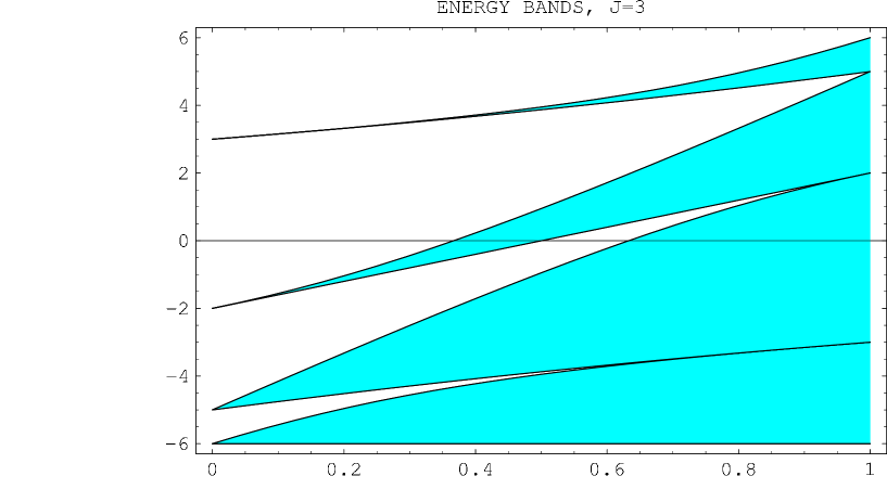
Figure 4: The energy bands for the Lamé system (1), as a function of $\nu$. The plot given is for $J=3$. The first (from the bottom) and the third allowed bands (unshaded) are of the p-ap type, while the second and the fourth ones of the ap-p type, see text.

4.3 $J=4$, nine band-edge levels

According to the results of Sec. 3.1, the QES sector consists of one triplet ($j=1$) and three doublets ($\tilde{j}=1/2$). The triplet is obtained from Eq. (41),

$$E_{1,5,9} = -\frac{10}{3}\,(1-2\nu)-\frac{8\sqrt{13}}{3}\,\sqrt{1-\nu+\nu^{2}}\,\cos\left[\delta_{1,5,9}\right.$$

$$- \left.\!\!\!\!\frac{1}{3}\,{\rm arcsin}\frac{3\sqrt{3}\,\sqrt{144-432\nu+2089\nu^{2}-3458\nu^{3}+2089\nu^{4}-432\nu^{5}+144\nu^{6}}}{26\sqrt{13}\,(1-\nu+\nu^{2})^{3/2}}\,\,\right],$$

$$\delta_{1} = \frac{\pi}{3}\,,\qquad\delta_{5}=-\frac{\pi}{3}\,,\qquad\delta_{9}=\pi\,.$$ (61)

At $\nu<1/2$, the arcsine on the right-hand side is in the first quadrant, and is defined in a standard way. At $\nu>1/2$ it must be defined as a smooth analytic continuation.

The doublet levels are obtained from Eqs. (44), (47) and (48),

$$E_{4} = 5\nu-2\sqrt{9-9\nu+4\nu^{2}}\,,$$

$$E_{8} = 5\nu+2\sqrt{9-9\nu+4\nu^{2}}\,,$$ (62)

and

$$E_{3} = -5+10\nu-2\sqrt{4-9\nu+9\nu^{2}}\,,$$

$$E_{7} = -5+10\nu+2\sqrt{4-9\nu+9\nu^{2}}\,,$$ (63)

and

$$E_{2} = -5+5\nu-2\sqrt{4+\nu+4\nu^{2}}\,,$$

$$E_{6} = -5+5\nu+2\sqrt{4+\nu+4\nu^{2}}\,.$$ (64)

The triplet levels (61) are dual, and so are the doublet levels $E_{3}$ and $E_{7}$. Moreover, the two remaining doublets are dual to each other, namely $E_{4}$ is dual to $E_{6}$, while $E_{8}$ to $E_{2}$, see Fig. 5.

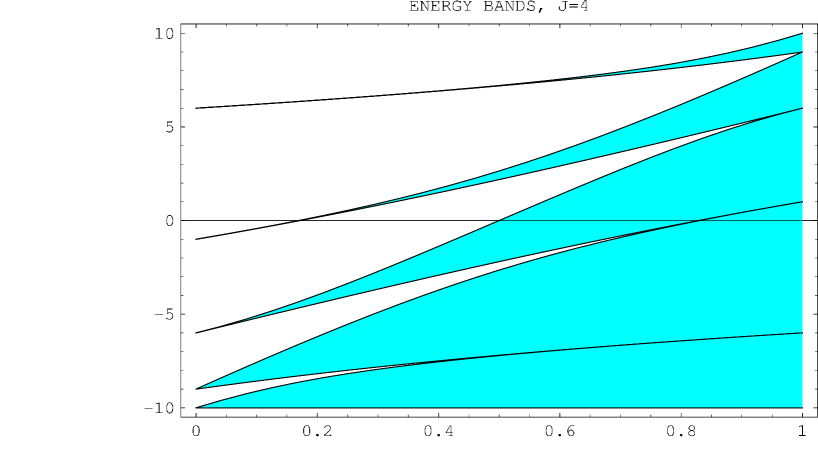
Figure 5: The energy bands for the Lamé system (1), as a function of $\nu$. This is the plot for $J=4$. The first (the lowest), the third and the fifth allowed bands (unshaded) are of the p-ap type, while the second and the fourth of the ap-p type, see text.

4.4 $J=5$, eleven band-edge levels

According to the results of Sec. 3.2 the QES sector consists three triplets ($j=1$) and one doublet ($\tilde{j}=1/2$).

The triplet levels are obtained from Eqs. (52), (55) and (56). It is not difficult to obtain that

$$E_{1,5,9} = \frac{5}{3}\,(-5+7\nu)-\frac{8}{3}\,\sqrt{13-13\nu+28\nu^{2}}\,\cos\Big{[}\delta_{1,5,9}$$

$$- \left.\!\!\!\!\frac{1}{3}\,{\rm arcsin}\frac{9\sqrt{3}\,\sqrt{16-48\nu+461\nu^{2}-842\nu^{3}+541\nu^{4}-128\nu^{5}+256\nu^{6}}}{2(13-13\nu+28\nu^{2})^{3/2}}\,\,\right],$$

$$\delta_{1} = \frac{\pi}{3}\,,\qquad\delta_{5}=-\frac{\pi}{3}\,,\qquad\delta_{9}=\pi\,.$$ (65)

This triplet is dual to that of Eq. (67). As in Eq. (61), the arcsine on the right-hand side is defined in the standard way when it is in the first quadrant, (i.e. at $\nu<\nu_{*}=0.371...$) while at larger $\nu$ the arcsine is understood as a smooth analytic continuation .

Furthermore,

$$E_{2,6,10} = -\frac{10}{3}\,(1-2\nu)-\frac{8}{3}\,\sqrt{28-13\nu+13\nu^{2}}\,\cos\Big{[}\delta_{2,6,10}$$

$$- \left.\!\!\!\!\frac{1}{3}\,{\rm arcsin}\frac{9\sqrt{3}\,\sqrt{256-128\nu+541\nu^{2}-842\nu^{3}+461\nu^{4}-48\nu^{5}+16\nu^{6}}}{2\,(28-13\nu+13\nu^{2})^{3/2}}\,\,\right],$$

$$\delta_{2} = \frac{\pi}{3}\,,\qquad\delta_{6}=-\frac{\pi}{3}\,,\qquad\delta_{10}=\pi\,.$$ (66)

This triplet of levels is dual to itself.

Finally, the third triplet is

$$E_{3,7,11}=\frac{5}{3}\,(-2+7\nu)-\frac{8}{3}\,\sqrt{28-43\nu+28\nu^{2}}\,\cos\Big{[}\delta_{3,7,11}$$

$$-\,\,\left.\!\!\!\!\frac{1}{3}\,{\rm arcsin}\frac{9\sqrt{3}\,\sqrt{256-1408\nu+3741\nu^{2}-5162\nu^{3}+3741\nu^{4}-1408\nu^{5}+256\nu^{6}}}{2(28-43\nu+28\nu^{2})^{3/2}}\,\right],$$

$$\delta_{3}=\frac{\pi}{3}\,,\qquad\delta_{7}=-\frac{\pi}{3}\,,\qquad\delta_{11}=\pi\,.$$ (67)

It is dual to the triplet (65).

The doublet levels are obtained from Eq. (54),

$$E_{4} = -5+10\nu-6\sqrt{1-\nu+\nu^{2}}\,,$$

$$E_{8} = -5+10\nu+6\sqrt{1-\nu+\nu^{2}}\,.$$ (68)

These two eigenvalues are dual to each other. The overall band structure for $J=5$ is presented in Fig. 6.

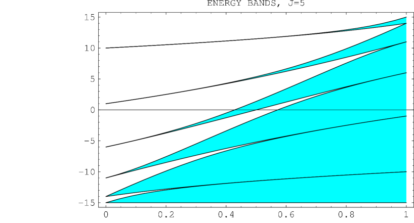
Figure 6: The energy bands for the Lamé system (1), as a function of $\nu$. This is the plot for $J=5$. The first (the lowest), the third and the fifth allowed bands (unshaded) are of the p-ap type, while the second, the fourth and the sixth of the ap-p type, see text.

4.5 The general pattern

The remarkable features of duality and energy-reflection symmetry of the spectral problem (1) reveal themselves in a transparent manner in Figs. 2, 4, 5 and 6. The allowed bands of the elliptic potential $\nu\,{\rm sn}^{2}(\phi|\nu)$ present (up to a sign) the forbidden bands (gaps) of the potential $(1-\nu)\,{\rm sn}^{2}(\phi|1-\nu)$, and vice versa. A nice illustration for duality of this type was given long ago by M. Escher. Figure 7 shows a fragment of Escher’s “Sky and Water.” Here the gaps between the birds are fishes, while the gaps between the fishes are birds.

Figure 7: An illustration of duality: a fragment of Escher’s “Sky and Water.”

The last allowed band extends up to $E=\infty$. The lower boundary of this band corresponds to periodic wave functions for even values of $J$, and to anti-periodic ones for odd values of $J$. The p-ap and ap-p allowed bands alternate, and so do the gaps. At $\nu=1/2$, the energy bands are self-dual. This means that for each band (gap) edge with the energy $E$ there is one with the energy $-E$.

As $\nu\to 1$, the widths of the allowed bands (except the last one) tend to zero. In fact, these bands shrink to the discrete bound states of the Pöschl-Teller system. The lowest band is at $E=-J(J-1)/2$, the last band starts at $E=J(J+1)/2$. On the contrary, the gap widths decrease. The width of the lowest gap is $\Delta E=2J-1$, and then it decreases: $\Delta E=2J-3,\,\,\,2J-5,....,1$.

As $\nu\to 0$, the gap widths tend to zero, while the allowed band widths grow. The lowest allowed band is at $-J(J+1)/2\leq E\leq-J(J+1)/2-1$, its width is $\Delta E=1$, the next band is at $-J(J+1)/2-1\leq E\leq-J(J+1)/2-4$, its width is $\Delta E=3$, and so on. The last (infinite-width) allowed band starts at $E=J(J-1)/2$. The bottom edge of the last (infinite-width) allowed band is of the p type for even $J$ and ap type for odd $J$.

In each $(2j+1)$-plet ($j>0$) of the $sl(2)$ representation (Sect. 3) the energy level pattern is as follows:

$$E_{k_{0}}\,,\,\,\,E_{k_{0}+4}\,,\,\,\,E_{k_{0}+8}\,,\dots\,.$$

The multiplet which includes $E_{J+1}$ is special: it is always self-dual. The $(J+1)$-th energy eigenvalue $E_{J+1}$ is dual to itself and passes through zero at $\nu=1/2$. The dimension of this multiplet is $2\,[J/4]+1$, where […] denotes the entire part.

The pattern described above is readily understood from the representation (3) and/or the $sl(2)$-based representations considered in Sect. 3.

5 Energy reflection symmetry at the self-dual
point $\nu=1/2$.

When $\nu=\frac{1}{2}$, the Lamé system is self-dual and so has an energy-reflection (ER) symmetry. This symmetry implies that each eigenlevel of energy $E$ is accompanied by a level of energy $-E$, the corresponding wave functions being related in a well-defined manner. A class of ER symmetric QES problems was constructed in [7]. Although the construction of Ref. [7] guarantees ER-symmetric spectra, by no means does it present a sufficient condition for the ER symmetry. The spectral problem (1), with $\nu=1/2$, is in fact an expansion of the class of the ER-symmetric problems (the mechanism leading to this expansion, the possibility of different algebraizations of one and the same spectral problem due to the existence of distinct solutions for the quasi-gauge, was overlooked in [7]). The focus of this section is the ER symmetry properties of periodic elliptic potentials from the standpoint of QES, and their connection with the Lamé system (1).

To begin, we observe that at $\nu=1/2$ the function sn${}^{2}(\phi|\nu)$ is related to the Weierstrass function ${\cal P}$ with the invariants [13]

$$g_{2}=4\,,\qquad g_{3}=0\,;$$ (69)

namely,

$$\frac{J(J+1)}{2}\,\left\{{\rm sn}^{2}(\phi|\nu)-1\right\}\equiv-\,\frac{J(J+1)}{2}\,\,\frac{1}{{\cal P}\left(\frac{\phi}{\sqrt{2}}-\frac{\tau}{2}\right)},$$ (70)

where

$$\tau=\frac{2\sqrt{\pi}\Gamma(5/4)}{\Gamma(3/4)}$$ (71)

is the period of the Weierstrass function ${\cal P}(x;\,g_{2}=4,g_{3}=0)$. The invariants $g_{2,3}$ will be suppressed below. This relation implies, in turn, that at $\nu=1/2$ the spectral problem (1) can be written as

$$\left\{-\frac{1}{2}\,\frac{d^{2}}{dx^{2}}-\frac{J(J+1)}{2}\,\,\frac{1}{{\cal P}\left(x-\frac{\tau}{2}\right)}\right\}\Psi(x)=E\,\Psi(x)\,,$$ (72)

where the following change of variables is made:

$$\frac{\phi}{\sqrt{2}}\to x\,.$$ (73)

Note the occurrence of the factor $1/2$ in the kinetic term. Weierstrass function related potentials first surfaced in the context of the Lie-algebraic construction in [1, 10], and are well known in the general study of finite-gap potentials [15].

In the general case of sn$(\phi|\nu)$ the parallelogram of periods is a rectangle; the $\nu=1/2$ case is special: the parallelogram of periods is a square. This is called the ”lemniscate” case [13]. The auxiliary variable $\eta(\phi)=1-{\rm sn}^{2}(\phi|\nu)$ (see Eq. (13)) becomes

$$\eta(x)\equiv\frac{1}{{\cal P}(x)}\,.$$ (74)

The analogue of Eq. (12) becomes

$$\left(\frac{d\,\eta}{d\,x}\right)^{2}=4(\eta-\eta^{3})\,.$$ (75)

A crucial relation

$$\eta(ix)=-\eta(x)$$ (76)

follows from the properties of the Weierstrass function with the invariants (69). For real $x$ the function $\eta(x)$ varies in the interval $[0,1]$; it is doubly periodic in the complex plane (along the real and imaginary axes), with periods $\tau$ and $i\tau$. An example of the ER-symmetric potential (72) ($J=5$), with the corresponding band structure, is shown in Fig. 8.

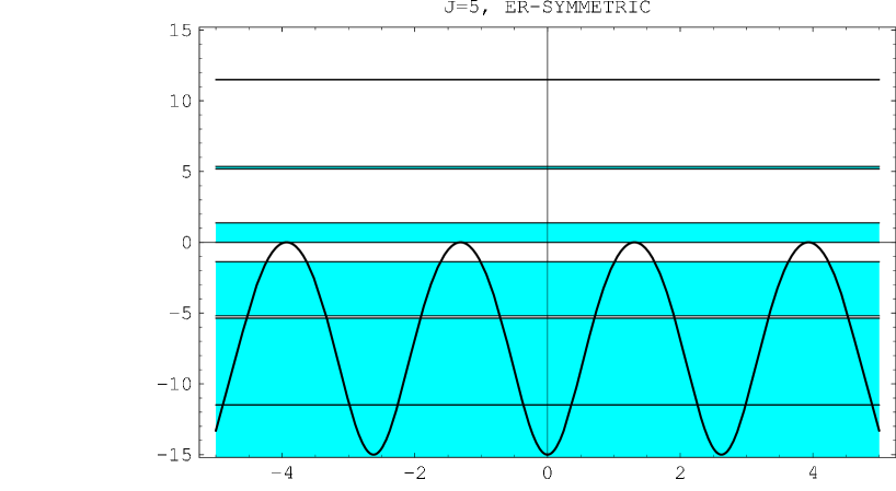
Figure 8: The ER-symmetric potential (72) versus $x$ for $J=5$. The gaps are shaded while the allowed bands are unshaded. Notice the ER symmetry which interchanges bands and gaps under $E\to-E$.

5.1 J even, self-dual level multiplets

Two solutions of this type for the band edges (i.e. individually ER-symmetric) were found some time ago in Ref. [7] (see Eq. (17) with $\nu=0$ and $1/2$). The first one (periodic eigenfunctions, cf. Eq. (41)) is

$$j = \frac{J}{4}\,,\qquad\Psi(x)=P_{2j}(\eta(x))\,,$$ (77)

$$H = -2(\eta-\eta^{3})d^{2}_{\eta}+(3\eta^{2}-1)d_{\eta}-2j(4j+1)\eta$$ (78)

$$= -2T^{+}T^{0}-2T^{0}T^{-}-(6j+1)T^{+}-(2j+1)T^{-}\,.$$

The second solution (anti-periodic eigenfunctions, cf. Eq. (47)) is

$$\tilde{j} = \frac{J-2}{4}\,,\qquad\Psi(x)=\sqrt{1-[\eta(x)]^{2}}\,\,P_{2\tilde{j}}\,(\eta(x))\,,$$

$$H_{``G"} = -2(\eta-\eta^{3})d^{2}_{\eta}+(7\eta^{2}-1)d_{\eta}-2\tilde{j}(4\tilde{j}+5)\eta$$ (79)

$$= -2T^{+}T^{0}-2T^{0}T^{-}-(6\tilde{j}+5)T^{+}-(2\tilde{j}+1)T^{-}\,.$$

Note that the ER symmetry of each of the two level multiplets above follows from the fact that

$$H\to-H$$

under the replacement $x\to ix,\,\,\,\eta\to-\eta$. The corresponding wave functions are obtained from one another by the replacement $\eta\to-\eta$. This is the mechanism discussed in [7]. In the example of Sec. 4.3, $J=4$, the band edges under discussion are

$$\{2\sqrt{13}\,,\,\,\,0\,,\,\,\,-2\sqrt{13}\}\,,\qquad\{\sqrt{7},\,\,\,-\sqrt{7}\}\,.$$

5.2 J even, a level multiplet of the p type dual to that of the ap type

Our assertion is: there exists another mode in which the ER symmetry can be realized in the problem (1). It does not fall into the category specified by Eqs. (6) and (8) in Ref. [7]. We consider two distinct quasigauge transformations, both leading to Lie-algebraic $H_{``G"}$’s, such that the quasiphase factors $e^{-a}$ are not invariant under $\eta\to-\eta$, but, rather, are transformed one into another. This will lead to a wider class of ER-symmetric problems than that considered in Ref. [7]. The pair of conjugate Hamiltonians is

$$\tilde{j} = \frac{J-2}{4}\,,\qquad\Psi(x)=\sqrt{\eta(x)\left\{1-\eta(x)\right\}}\,\,P_{2\tilde{j}}\,(\eta(x))\,,$$

$$H_{``G"} = -2T^{+}T^{0}-2T^{0}T^{-}-2\left(3\tilde{j}+\frac{5}{2}\right)T^{+}-\left(2\tilde{j}+3\right)T^{-}$$ (80)

$$+ 2T^{0}+\left(2\tilde{j}+\frac{3}{2}\right)\,,$$

(periodic eigenfunctions, cf. Eq. (44)), and

$$\tilde{j} = \frac{J-2}{4}\,,\qquad\Psi(x)=\sqrt{\eta(x)\left\{1+\eta(x)\right\}}\,\,P_{2\tilde{j}}\,(\eta(x))\,,$$

$$H_{``G"} = -2T^{+}T^{0}-2T^{0}T^{-}-2\left(3\tilde{j}+\frac{5}{2}\right)T^{+}-\left(2\tilde{j}+3\right)T^{-}$$ (81)

$$- 2T^{0}-\left(2\tilde{j}+\frac{3}{2}\right)\,,$$

(anti-periodic eigenfunctions, cf. Eq. (48)).

The terms containing $T^{0}$ would be forbidden by the ansatz considered in Ref. [7]. However, it is clear that the Hamiltonians (80) and (81) swap under the substitution $\eta\to-\eta$. In the example of Sec. 4.3, $J=4$, the band edges under discussion are

$$\left\{\frac{5}{2}+\sqrt{22}\,,\,\,\,\frac{5}{2}-\sqrt{22}\right\},\,\,\,\mbox{periodic}\,;\qquad\left\{-\frac{5}{2}-\sqrt{22}\,,\,\,\,-\frac{5}{2}+\sqrt{22}\right\},\,\,\,\mbox{anti-periodic}\,.$$

5.3 J odd, self-dual level multiplets

Two solutions of the self-conjugate type for the band edges are as follows:

$$j = \frac{J-1}{4}\,,\qquad\Psi(x)=\sqrt{\eta(x)}\,\,P_{2j}\,(\eta(x))\,,$$

$$H_{``G"} = -2T^{+}T^{0}-2T^{0}T^{-}-2\left(3j+\frac{3}{2}\right)T^{+}-\left(2j+3\right)T^{-}\,,$$ (82)

(anti-periodic eigenfunctions, cf. Eq. (55)), and

$$\tilde{j} = \frac{J-3}{4}\,,\qquad\Psi(x)=\sqrt{\eta(x)\left[1-(\eta(x))^{2}\right]}\,\,P_{2\tilde{j}}\,(\eta(x))\,,$$

$$H_{``G"} = -2T^{+}T^{0}-2T^{0}T^{-}-2\left(3\tilde{j}+\frac{7}{2}\right)T^{+}-\left(2\tilde{j}+3\right)T^{-}\,.$$ (83)

(periodic eigenfunctions, cf. Eq. (54)). These two solutions fall into the category treated in Ref. [7]. In the example of Sec. 4.4, $J=5$, the band edges under discussion are

$$\{2\sqrt{33},\,\,\,0,\,\,\,-2\sqrt{33}\},\,\,\,\mbox{anti-periodic};$$

$$\{3\sqrt{3},\,\,\,-3\sqrt{3}\},\,\,\,\mbox{periodic}\,.$$

5.4 J odd, a level multiplet of the p type dual to that of the ap type

The pair of conjugate Hamiltonians is

$$j = \frac{J-1}{4}\,,\qquad\Psi(x)=\sqrt{1+\eta(x)}\,\,P_{2j}\,(\eta(x))\,,$$

$$H_{``G"} = -2T^{+}T^{0}-2T^{0}T^{-}-2\left(3j+\frac{3}{2}\right)T^{+}-\left(2j+1\right)T^{-}$$ (84)

$$- 2T^{0}-\left(2j+\frac{1}{2}\right)\,,$$

(periodic eigenfunctions, cf. Eq. (52)), and

$$j = \frac{J-1}{4}\,,\qquad\Psi(x)=\sqrt{1-\eta(x)}\,\,P_{2j}\,(\eta(x))\,,$$

$$H_{``G"} = -2T^{+}T^{0}-2T^{0}T^{-}-2\left(3j+\frac{3}{2}\right)T^{+}-\left(2j+1\right)T^{-}$$ (85)

$$+ 2T^{0}+\left(2j+\frac{1}{2}\right)\,,$$

(anti-periodic eigenfunctions, cf. Eq. (56)). In the example of Sec. 4.4, $J=5$, the band edges under discussion are

$$\left\{-\frac{5}{2}-4\sqrt{6}\cos\left(\delta_{1,5,9}-\frac{\pi}{3}+\frac{1}{3}{\rm arcsin}\sqrt{\frac{191}{216}}\right)\approx-11.49,\,-1.37,\,5.36\right\},\,\,\,\mbox{p};$$

$$\left\{\frac{5}{2}+4\sqrt{6}\cos\left(\delta_{3,7,11}-\frac{\pi}{3}+\frac{1}{3}{\rm arcsin}\sqrt{\frac{191}{216}}\right)\approx-5.36,\,1.37,\,11.49\right\},\,\,\,\mbox{a-p}.$$

6 Weak coupling versus quasiclassical expansion

In this section we describe how the duality transformation (5) connects various perturbative and nonperturbative techniques, by relating information about states high up in the spectrum to states low down in the spectrum. We first consider approximate techniques for the locations of bands and gaps. Next we consider techniques for evaluating the widths of bands and gaps. The calculations of widths are sensitive to exponentially small contributions which are neglected in the calculations of the locations.

6.1 Estimates of locations of bands and gaps

Because of the duality transformation (5), the location of a low-lying band in the spectrum is related to the location of a high-lying gap in the dual spectrum (i.e., the spectrum for the potential obtained by making the duality replacement $\nu\to 1-\nu$). The location of the low-lying bands can be obtained by applying the weak coupling expansion. The location of a high-lying gaps can be obtained by applying the quasiclassical expansion. In both cases the quadratic Casimir $J(J+1)$ determines the expansion parameter. It is convenient to introduce a parameter $\kappa$,

$$\kappa=\sqrt{J(J+1)}\,.$$ (86)

Then $1/\kappa$ is the weak coupling constant of the perturbative expansion. Simultaneously, $1/\kappa$ plays the role of $\hbar$ in the quasiclassical expansion.

6.1.1 Perturbation theory for location of lowest band

In the limit $J\to\infty$, the width of the lowest band becomes very narrow, so it makes sense to estimate the “location” of the band. In fact, as we will see in the next sections, the width shrinks exponentially fast, so we can estimate the location of the band to within exponential accuracy using elementary perturbation theory. That is, for large $J$, we can consider a single isolated well of the periodic Lamé potential, and expand [13] near $\phi=0$, keeping quartic, sextic and higher order anharmonic terms,

$${\rm sn}^{2}(\phi|\nu)=\phi^{2}-\frac{\nu+1}{3}\phi^{4}+\frac{2+13\nu+2\nu^{2}}{45}\phi^{6}+\dots\,.$$ (87)

Rescaling the coordinate,

$$\phi=\frac{x}{(\nu J(J+1))^{1/4}}\equiv\nu^{-1/4}\,\kappa^{-1/2}\,x\,,$$

the Lamé equation (1) becomes

$$\left[-\frac{d^{2}}{dx^{2}}+x^{2}-\frac{\nu+1}{3\kappa\,\sqrt{\nu}}\,x^{4}+\frac{2+13\nu+2\nu^{2}}{45\kappa^{2}\,\nu}\,x^{6}+\dots\right]\,\Psi=\frac{E+\frac{1}{2}\kappa^{2}}{\kappa\,\sqrt{\nu}}\,\,\Psi\,.$$ (88)

Thus, the lowest energy level can be evaluated as a simple series in powers of $1/\kappa$,

$$E_{0}=-\frac{1}{2}\,\kappa^{2}\left[1-\frac{2\sqrt{\nu}}{\kappa}+\frac{\nu+1}{2\,\kappa^{2}}+\frac{(1-4\nu+\nu^{2})}{8\,\sqrt{\nu}\,\kappa^{3}}+O\left(\frac{1}{\kappa^{4}}\right)\right]\,.$$ (89)

6.1.2 Semiclassical method for location of highest gap

As $J\to\infty$, the location of the highest gap can be found by semiclassical techniques. First, note that for a given $\nu$, as $J\to\infty$ the highest gap lies above the top of the potential. Thus, the turning points lie off the real $\phi$ axis. For a periodic potential the gap edges occur when the discriminant [16, 21] takes values $\pm 1$. By WKB, the discriminant is

$$\Delta(E)=\cos\left(\frac{1}{\hbar}\,\,\sum_{n=0}^{\infty}\,\hbar^{n}\,S_{n}\,(P)\right)\,,$$ (90)

where $P$ is the period, and the $S_{n}(x)$ are the standard WKB functions (see e.g. [22]),

$$S_{0}(x) = \int^{x}_{0}\sqrt{Q(t)}\,dt\,,$$

$$S_{1}(x) = -\frac{1}{4}\left[\log Q(x)\right]_{0}^{x}\,,$$

$$S_{2}(x) = \int^{x}_{0}\left[\frac{Q^{\prime\prime}}{8Q^{3/2}}-\frac{5(Q^{\prime})^{2}}{32\,Q^{5/2}}\right]\,dt\,,$$

$$S_{3}(x) = \left[-\frac{Q^{\prime\prime}}{16Q^{2}}+\frac{5(Q^{\prime})^{2}}{64\,Q^{3}}\right]_{0}^{x}\,,$$ (91)

and so on. Here

$$Q(x)\equiv E-V(x)\,.$$

These functions $S_{n}(x)$ can be generated to any order by a simple recursion formula [22]. The $J$-th gap occurs when the argument of the cosine in the discriminant (90) is $J\pi$. This gives the location of the $J$-th gap, neglecting exponential corrections which correspond to the exponentially narrow width of the gap in the semiclassical $J\to\infty$ limit.

For the Lamé system, we rescale the Lamé equation (1) as

$$-\frac{1}{\kappa^{2}}\,\frac{d^{2}}{d\phi^{2}}\,\psi+\nu\,{\rm sn}^{2}(\phi|\nu)\,\psi=\left(\frac{E}{\kappa^{2}}+\frac{1}{2}\right)\,\psi\,,$$ (92)

and, thus, identify $\hbar$ in Eq. (90) as

$$\frac{1}{\kappa}\leftrightarrow\hbar\,.$$ (93)

As a result, the condition for the occurrence of the $J$-th gap takes the form

$$\kappa\,\,\sum_{n=0}^{\infty}\,\frac{1}{\kappa^{n}}\,{S_{n}\,(2K)}=J\,\pi=\pi\,\kappa\left(1-\frac{1}{2\,\kappa}+\frac{1}{8\,\kappa^{2}}-\frac{1}{128\,\kappa^{4}}+\dots\right)\,,$$ (94)

where $2K$ is the period of the Lamé potential, and where on the right-hand side we have expressed $J$ in terms of the effective semiclassical expansion parameter $1/\kappa$. This relation (94) can be used to find an expansion for the energy of the $J$-th gap by expanding

$$E=\frac{1}{2}\,\kappa^{2}+\sum_{\ell=1}^{\infty}\,\frac{\varepsilon_{\ell}}{\kappa^{\ell-2}}\,.$$ (95)

The expansion coefficients $\varepsilon_{l}$ are fixed by identifying terms on both sides of the expansion in (94). For example, the leading terms clearly match because

$$S_{0}\,(2K) = \int_{0}^{2K}\sqrt{\frac{E}{\kappa^{2}}+\frac{1}{2}-\nu\,{\rm sn}^{2}(\phi|\nu)}\,\,d\phi$$ (96)

$$= \int_{0}^{2K}\sqrt{1-\nu\,{\rm sn}^{2}(\phi|\nu)}\,\,d\phi+O\left(\frac{1}{\kappa}\right)$$

$$= \pi+O\left(\frac{1}{\kappa}\right)\,.$$

The next-to-leading term on the left-hand-side of the expansion (94) comes from expanding $S_{0}(2K)$:

$$S_{0}\,(2K) = \int_{0}^{2K}\sqrt{1-\nu\,{\rm sn}^{2}(\phi|\nu)+\frac{\varepsilon_{1}}{\kappa}}\,\,d\phi+\dots$$ (97)

$$= \pi+\frac{\pi\,\varepsilon_{1}}{2\kappa\,\sqrt{1-\nu}}+O\left(\frac{1}{\kappa^{2}}\right)\,.$$

Matching the next-to-leading terms in (94), we find

$$\varepsilon_{1}=-\sqrt{1-\nu}\,.$$ (98)

This agrees with the next-to-leading term in the perturbative expansion (89), after making the duality transformations $\nu\to 1-\nu$ and $E\to-E$.

Note that there is no contribution from $S_{1}$, since $Q(x)$ is periodic with period $2K$. (It is important here that the turning points are off the real axis, so that integrating along the real period we do not encounter any turning points, which would then require deformation of the integration contour in the complex plane [23, 22]). Indeed, for the same reason, none of the odd-indexed $S_{n}$ contributes to the discriminant.

Similarly, successive orders in the energy expansion (95) follow by expanding (94) to a given order in $1/\kappa$, and matching to determine the expansion coefficients $\varepsilon_{\ell}$. In this way one finds

$$E=\frac{1}{2}\,\kappa^{2}-\kappa\,\sqrt{1-\nu}+\frac{2-\nu}{4}+\frac{(-2+2\nu+\nu^{2})}{16\,\kappa\,\sqrt{1-\nu}}+\dots\,.$$ (99)

Comparing with the perturbative expansion (89) we see that the semiclassical expansion (99) is indeed the dual of the perturbative expansion (89), under the duality transformation $\nu\to 1-\nu$ and $E\to-E$.

6.2 Estimates of widths of bands and gaps

The semiclassical techniques used in the previous section were not sensitive to the exponentially small corrections needed to estimate the width of a low-lying band, or a high-lying gap. Yet, by the duality transformation (5), the width of the lowest band is equal to the width of the highest gap, for the dual potential obtained by making the replacement $\nu\to 1-\nu$. In this section we compute the widths of the lowest band and highest gap, using various approximate techniques, and compare with the exact duality result. This provides a link between perturbative and non-perturbative techniques that is much more sensitive than that discussed in the previous section for the locations of low-lying bands and high-lying gaps.

6.2.1 Algebraic approach for width of lowest band

Since the band edge energies are given by the eigenvalues of the finite dimensional matrix $H$ in (3), the most direct way to evaluate the width of the lowest-lying band is to take the difference of the two smallest eigenvalues of $H$. For any given value of the elliptic parameter $\nu$, this involves finding the eigenvalues of a $(2J+1)\times(2J+1)$ matrix, which can be done with great precision. However, finding the eigenvalues as functions of $\nu$ (see, for example, the plots in Figs. 2, 4, 5 and 6 for $J=2$ and $J=5$) rapidly becomes complicated as $J$ increases. Nevertheless, from these expressions it is possible to deduce [20] the exact leading behavior, in the limit $\nu\to 1$, of the width of the lowest band, for any $J$ :

$$\Delta E^{\rm algebraic}_{\rm band}={8J\,\Gamma(J+1/2)\over 4^{J}\sqrt{\pi}\,\Gamma(J)}\,(1-\nu)^{J}\,\left(1+\frac{J-1}{2}(1-\nu)+\dots\right)$$ (100)

This clearly shows the exponentially narrow character of the lowest band in the $\nu\to 1$ limit.

6.2.2 Tight-binding approximation for width of lowest band

In the tight-binding approximation [21], one assumes the periodic wells are far separated, so that the periodic potential can be treated as a periodic sequence of “atomic” wells, each of which has a set of discrete bound levels. Small overlap effects broaden these discrete bound levels into bound bands. In the Lamé case this approximation can be made very explicit due to the remarkable elliptic function identity:

$$\nu\,{\rm sn}^{2}(\phi|\nu)=\frac{E^{\prime}}{K^{\prime}}-\left(\frac{\pi}{2K^{\prime}}\right)^{2}\sum_{n=-\infty}^{\infty}\left[{\rm sech}\left(\frac{\pi}{2K^{\prime}}(\phi-2nK)\right)\right]^{2}\,.$$ (101)

Here $E(\nu)$ is the complete elliptic integral of the second kind [12, 13], and

$$E^{\prime}(\nu)=E(1-\nu)\,.$$

This identity (101) shows that the periodic Lamé potential can be written as a sequence of periodically displaced (by the period $2K(\nu)$) Pöschl-Teller “atomic” wells (but the rescaling factor $\frac{\pi}{2K^{\prime}}$ is non-obvious). This “atomic” structure becomes clear graphically as $\nu\to 1$ (see Fig. 1), but is in fact true for all $\nu$. Since each “atomic” well is a Pöschl-Teller well, the normalized lowest energy bound state is

$$\Psi_{0}(\phi)=\sqrt{\frac{\sqrt{\pi}\,\Gamma(J+1/2)}{2K^{\prime}\,\Gamma(J)}}\,\,\left[{\rm sech}\left(\frac{\pi}{2K^{\prime}}\,\phi\right)\right]^{J}\,.$$ (102)

In the tight-binding (TB) approximation, the energy of this lowest state broadens into a band of width [20, 21]

$$\Delta E^{\rm TB}_{\rm band}\!\! = \!\!4\kappa^{2}\left(\frac{\pi}{2K^{\prime}}\right)^{2}\int_{-\infty}^{\infty}d\phi\sum_{n\neq 0}\left[{\rm sech}\left(\frac{\pi(\phi-2nK)}{2K^{\prime}}\right)\right]^{2}\,\Psi_{0}(\phi)\Psi_{0}(\phi-2K)$$ (103)

$$\approx {8J\,\Gamma(J+1/2)\over 4^{J}\sqrt{\pi}\,\Gamma(J)}\,\,(1-\nu)^{J}\,\left(1+\frac{J-1}{2}(1-\nu)+\dots\right)\,,$$

where in the second line we have kept dominant terms as $\nu\to 1$, and used the fact that

$$\exp\left(-\pi\frac{K}{K^{\prime}}\right)\sim\frac{1-\nu}{16}\left(1+\frac{1}{2}(1-\nu)+\dots\right)\,.$$

This result (103) agrees precisely with the exact result (100) to this order in $1-\nu$. Therefore, for any $J$, the tight-binding approximation is good as $\nu\to 1$; i.e. as the separation between atomic wells becomes large.

6.2.3 Instanton approximation for width of lowest band

In the instanton approximation [24], tunneling is suppressed because the barrier height is much greater than the ground state energy of any given isolated “atomic” well. For the Lamé potential in (1), this means

$$\kappa\,\sqrt{\nu}\gg 1\,.$$ (104)

Remarkably, the instanton calculation for the Lamé potential can be done in closed form [20], leading to

$$\Delta E^{\rm instanton}_{\rm band}=\frac{16}{\sqrt{\pi}}\,\left(\kappa^{2}\,\nu\right)^{3/4}\,\left(1+\sqrt{\nu}\right)^{-2\kappa}\,\left(1-\nu\right)^{\kappa-\frac{1}{2}}\,.$$ (105)

To compare this instanton result (105) with the algebraic result (100) we take $\nu\to 1$, and we take $J$ to be large, in order to be in the semiclassical limit (104). Then

$$\Delta E^{\rm instanton}_{\rm band}\sim\frac{8J^{3/2}}{\sqrt{\pi}\,4^{J}}\,\,\left(1-\nu\right)^{J}\left[1+\frac{J-1}{2}(1-\nu)+\dots\right]\,,$$ (106)

which agrees perfectly with the large $J$ limit (using Stirling’s formula) of the exact algebraic result (100). Thus, this example gives an analytic confirmation that the instanton calculation gives the correct leading large $J$ behavior of the width of the lowest band, as $\nu\to 1$. For other values of $\nu$, the instanton formula (105) is also the correct leading large $J$ result, but the comparison with $\Delta E^{\rm algebraic}_{\rm band}$ must be done numerically [20] for a given value of $\nu$ since the large $J$ asymptotic behavior of $\Delta E^{\rm algebraic}_{\rm band}$ for arbitrary $\nu$ is not analytically calculable.

6.2.4 WKB approximation for width of lowest band

We can also estimate the width of the lowest band using WKB. First, rescale the the Lamé equation (1) as

$$-\frac{1}{2}\,\frac{1}{\kappa^{2}\,\nu}\,\frac{d^{2}\Psi}{d\phi^{2}}+\frac{1}{2}\,{\rm sn}^{2}\,(\phi|\nu)\,\Psi(\phi)=\left(\frac{1}{4\nu}+\frac{E}{2\,\kappa^{2}\,\nu}\right)\Psi(\phi)\equiv{\cal E}\,\Psi(\phi)\,.$$ (107)

In this form we clearly see the small WKB parameter to be

$$``\hbar"=\frac{1}{\kappa\,\sqrt{\nu}}\,,$$

so that the large $J$ limit is indeed semiclassical. Then, the standard WKB [25, 26, 20] expression for the band width is

$$\Delta{\cal E}^{\rm WKB}=\frac{2``\hbar"}{\pi}\,\exp\left(-\frac{1}{``\hbar"}\,\int_{\rm t.p.}\,d\phi\,\sqrt{2(V(\phi)-{\cal E})}\right)$$ (108)

where t.p. denotes the turning points. Thus, remembering to rescale the energy and using the first two terms in Eq. (89) for the energy of the lowest band, we get

$$\Delta E^{\rm WKB}_{\rm band}=\frac{4}{\pi}\,\kappa\,\sqrt{\nu}\,\exp\left\{-{\kappa\,\sqrt{\nu}}\,\int_{\rm t.p.}\,d\phi\,\sqrt{{\rm sn}^{2}(\phi|\nu)-\frac{1}{\kappa\,\sqrt{\nu}}}\,\right\}\,.$$ (109)

Defining $y={\rm sn}^{2}(\phi|\nu)$, we can now evaluate the integral in the semiclassical limit where $``\hbar"=1/(\kappa\,\sqrt{\nu})\ll 1$,

$$\int_{``\hbar"}^{1}\frac{\sqrt{1-``\hbar"/y}}{\sqrt{1-y}\sqrt{1-\nu\,y}}\,dy=\frac{1}{\sqrt{\nu}}\,\ln\left(\frac{1+\sqrt{\nu}}{1-\sqrt{\nu}}\right)$$

$$-``\hbar"\left(\frac{1}{2}\ln``\hbar"+\frac{1}{2}\ln\,(1-\nu)-2\ln 2-\frac{1}{2}\right)+O\left((``\hbar")^{2}\right)\,.$$ (110)

As a result, one finds [20] from (109)

$$\Delta E^{\rm WKB}_{\rm band} = \sqrt{\frac{e}{\pi}}\,\Delta E^{\rm instanton}_{\rm band}\,.$$ (111)

This factor of $\sqrt{e/\pi}$ has been known for a long time [27]. (The instanton result for $\Delta E_{\rm band}$ is correct while Eq. (109) is off by this factor.) It has been found in many other comparisons between the instanton method and the WKB formula (108) [26, 28, 29, 30]. It can be traced to a slightly crude matching of normalizations of wave functions [27, 31, 32]. A more precise WKB treatment leads, of course, to complete agreement between these two semiclassical methods, as has recently been emphasized explicitly for the Lamé potential [33].

6.2.5 Algebraic approach for width of highest gap

We now turn our attention to the width of the highest gap. Taking the difference of the two largest eigenvalues of the finite dimensional matrix $H$ in (3), it is straightforward to show that as $\nu\to 0$, for any $J$, this difference gives

$$\Delta E^{\rm algebraic}_{\rm gap}={8J\,\Gamma(J+1/2)\over 4^{J}\sqrt{\pi}\,\Gamma(J)}\,\nu^{J}\left(1+\frac{J-1}{2}\,\nu+\dots\right)\,,$$ (112)

which is the same as the algebraic expression (100) for the width of the lowest band, with the duality replacement $\nu\to 1-\nu$.

This result illustrates a theorem due to Trubowitz [34], which states that for a real analytic periodic potential, the gap widths shrink exponentially fast as one goes up in the spectrum. This in turn extends an earlier result of Hochstadt [35], which states that the gap widths go like $0(\frac{1}{l^{m}})$ if the potential is $m$ times differentiable. For a real analytic potential, such as the Lamé potential in (1), the gap widths shrink faster than any power of the gap label $l$, and, in fact, shrink exponentially. By duality, the low-lying bands are also exponentially narrow, as in (100).

6.2.6 Naive perturbative estimate for width of highest gap

As $\nu\to 0$, for fixed $J$, the potential in (1) becomes weak. Thus, one should be able to solve this problem using perturbation theory. Near $\nu=0$, the $n$-th gap can be considered as a splitting between the two degenerate free states $\Psi_{\pm}=\exp(\pm in\phi)$ at $E=n^{2}-\frac{1}{2}J(J+1)$. A standard solid state physics approximation gives [21] the width of the $n$-th gap as (twice) the $n$-th Fourier component of the potential,

$$\Delta E^{n}_{\rm gap}\approx 2|V_{n}|\,.$$ (113)

The Jacobi elliptic function has Fourier decomposition [12]

$$\nu\,{\rm sn}^{2}(\phi|\nu)=1-\frac{E(\nu)}{K(\nu)}+\frac{\pi^{2}}{K^{2}}\,\sum_{n=1}^{\infty}\,\,\frac{n\,\cos\left(\frac{n\pi\phi}{K}\right)}{\sinh\left(\frac{n\pi K^{\prime}}{K}\right)}\,.$$ (114)

Thus, for the highest (i.e., the $J$-th) gap, we would deduce

$$\Delta E^{J} \approx J(J+1)\,\frac{\pi^{2}}{K^{2}}\,\,\frac{J}{\sinh\left(\frac{J\pi K^{\prime}}{K}\right)}$$ (115)

$$\sim 8\,J^{2}(J+1)\,\left(\frac{\nu}{16}\right)^{J}\,,\qquad\nu\to 0\,.$$

When $J=1$, this agrees with the leading term in the exact algebraic result (112). But it does not agree when $J\geq 2$. This failure illustrates an important point – the formula (113) comes from first-order in perturbation theory. However, from (112) we see that the width of the highest gap is of $J$-th order in perturbation theory. So first-order perturbation theory is clearly not sufficient for $J\geq 2$. Indeed, to compare with the semi-classical (large $J$) results for the width of the lowest band, we see that we will have to be able to go to very high orders in perturbation theory. This is an interesting, and very direct, illustration of the well-known connection between non-perturbative physics and high orders of perturbation theory.

6.2.7 Perturbation theory to order $J$ for width of highest gap

It is generally very difficult to go to high orders in perturbation theory, even in quantum mechanics. For the Lamé system (1) we can exploit the algebraic relation to the finite-dimensional spectral problem (3). However, since $H$ in (3) is a $(2J+1)\times(2J+1)$ matrix, the large $J$ limit is still non-trivial. Since we are only interested in gap widths, in this section we neglect the constant term in $H$, and treat $\nu J_{y}^{2}$ as a perturbation of the free matrix $J_{x}^{2}$, which has eigenvalues $0,1^{2},2^{2},\dots,J^{2}$. The non-zero eigenvalues of $J_{x}^{2}$ are two-fold degenerate, while the zero eigenvalue is nondegenerate. We are interested in the splitting of the two degenerate eigenvectors of $J_{x}^{2}$ with the highest eigenvalue, $J^{2}$. Even though these two states are degenerate, they do not mix in perturbation theory, because of the form of the perturbation matrix $J_{y}^{2}$. This is essentially because both $J_{x}^{2}$ and $J_{y}^{2}$ have a sub-block structure in which alternate rows and columns separate. For definiteness, we choose the following $(2J+1)\times(2J+1)$ representation:

$$J_{x} = \frac{1}{2}\left(\matrix{0&\sqrt{2J}&0\cr\sqrt{2J}&0&\sqrt{2(2J-1)}&0\cr 0&\sqrt{2(2J-1)}&0&\sqrt{3(2J-2)}\cr&0&\ddots&\ddots&\ddots\cr&&&&&\sqrt{2J}\cr&&&0&\sqrt{2J}&0}\right),$$

$$J_{y} = -\frac{i}{2}\left(\matrix{0&\sqrt{2J}&0\cr-\sqrt{2J}&0&\sqrt{2(2J-1)}&0\cr 0&-\sqrt{2(2J-1)}&0&\sqrt{3(2J-2)}\cr&0&\ddots&\ddots&\ddots\cr&&&&&\sqrt{2J}\cr&&&0&-\sqrt{2J}&0}\right),$$

$$J_{z} = {\rm diag}\left(J,J-1,J-2,\dots,-J+2,-J+1,-J\right)\,.$$ (116)

Then the matrix elements of $J_{y}^{2}$ between the orthonormal eigenvectors of $J_{x}^{2}$ have the simple sparse structure

$$\tiny{\langle J_{y}^{2}\rangle=\left(\matrix{L_{1}&0&0&O_{0}&0&0&\dots&&&&&&&&0\cr 0&L_{2}&0&0&0&O_{1}&0&&&&&&&&\cr 0&0&L_{3}&0&0&0&O_{1}&0\cr O_{0}&0&0&D_{1}&0&0&0&O_{2}&0\cr 0&0&0&0&D_{1}&0&0&0&O_{2}&0\cr 0&O_{1}&0&0&0&D_{2}&0&0&0&\dots&0\cr&0&O_{1}&0&0&0&D_{2}&0&0&0&\ddots&0\cr&&0&O_{2}&0&0&0&\ddots&0&0&0&O_{J-3}&0&&\cr&&&0&O_{2}&0&0&0&\ddots&0&0&0&O_{J-3}&0&\cr&&&&0&\ddots&0&0&0&D_{J-3}&0&0&0&O_{J-2}&0\cr&&&&&0&\dots&0&0&0&D_{J-3}&0&0&0&O_{J-2}\cr&&&&&&0&O_{J-3}&0&0&0&D_{J-2}&0&0&0\cr&&&&&&&0&O_{J-3}&0&0&0&D_{J-2}&0&0\cr&&&&&&&&0&O_{J-2}&0&0&0&D_{J-1}&0\cr 0&&&&&&&&&0&O_{J-2}&0&0&0&D_{J-1}}\right)}$$

(117)

where the nonzero entries in the top left corner are

$$L_{1} = \frac{1}{2}J(J+1)\,,$$

$$L_{2} = \frac{1}{4}J(J+1)-\frac{1}{2}\,,$$

$$L_{3} = \frac{3}{4}J(J+1)-\frac{1}{2}\,.$$ (118)

The remaining diagonal entries appear in $2\times 2$ diagonal blocks, ${\rm diag}(D_{n},D_{n})$, with

$$D_{n}=\frac{1}{2}\,J(J+1)-\frac{1}{2}\,(n+1)^{2}\,,\qquad n=1,2,...,J-1\,.$$ (119)

Finally, the nonzero off-diagonal entries in (117) are

$$O_{0} = -\frac{1}{4}\sqrt{2J(J+2)(J^{2}-1)}\,,$$

$$O_{n} = -\frac{1}{4}\sqrt{(J-n)(J+n+2)(J^{2}-(n+1)^{2})}\,,\quad n=1,\dots,J-2\,.$$ (120)

In the basis used for (117), the last two rows and columns refer to the degenerate states with the highest eigenvalue of $J_{x}^{2}$. We see that there is indeed no string of matrix elements connecting $\langle J_{y}^{2}\rangle_{2J+1,2J+1}$ with $\langle J_{y}^{2}\rangle_{2J,2J}$. Thus, these two degenerate states do not mix at any order of perturbation theory.

Consider perturbing around the $(2J)$-th eigenstate of $J_{x}^{2}$, with eigenvalue $J^{2}$. The energy $E_{2J}$ of the perturbed system can be expressed implicitly as [36]

$$E_{2J}=E^{0}_{2J}+U_{2J,2J}+\sum_{n\neq 2J}\frac{U_{2J,n}U_{n,2J}}{E_{2J}-E^{0}_{n}}+\sum_{n\neq 2J}\sum_{m\neq 2J}\frac{U_{2J,n}U_{n,m}U_{m,2J}}{(E_{2J}-E^{0}_{n})(E_{2J}-E^{0}_{m})}+\dots$$

(121)

where $E^{0}_{n}$ is the $n$-th eigenvalue of the free system, and $U_{m,n}$ denotes the matrix element of the perturbation between the $m$-th and $n$-th free states. An analogous formula applies for $E_{2J+1}$.

¿From the $2\times 2$ sub-block structure of (117), it is clear that for the terms in (121) with strings of fewer than $J$ matrix element factors, the shifts in $E_{2J}$ and $E_{2J+1}$ are identical. Thus, these terms are irrelevant for the computation of the difference between $E_{2J}$ and $E_{2J+1}$. So, we can concentrate solely on the $J$-th order term in (121), which involves a product of exactly $J$ matrix element factors. Also, since we are looking for the leading term at this order of perturbation theory, we can replace the true eigenvalue $E_{2J}$ or $E_{2J+1}$ in the denominator by the free eigenvalue, which is $J^{2}$. A further simplification follows from the fact that there is only one nonzero string of $J$ matrix element factors beginning and ending with the index $2J$ or $2J+1$. Thus, to compute the difference $E_{2J+1}-E_{2J}$ at $J$-th order, we simply have to take the difference between the string of matrix elements in each case, with the appropriate denominator factor.

To proceed we need to specify whether $J$ is even or odd. We consider $J$ to be even (the case of $J$ odd only requires simple modifications, and is left to the reader). With $J$ even, there is in fact no nonzero string of $J$ matrix elements beginning and ending at $2J+1$. However, there is such a string beginning and ending at $2J$,

$$\left[U_{2J,2J-4}U_{2J-4,2J-8}\dots U_{8,4}U_{4,1}\right]^{2}=2\prod_{l=1,3,\dots,J-1}\left[\left(\frac{1}{4}\right)^{2}l(l+1)(2J+1-l)(2J-l)\right]$$

$$=\frac{2}{4^{J}}\left[J!(2J)(2J-1)(2J-2)\dots(J+2)(J+1)\right]=\frac{2(2J)!}{4^{J}}\,.$$ (122)

This, together with a factor of $\nu^{J}$, gives the numerator of the $J$-th order term in the perturbation series (121). The denominator of the $J$-th order term, with $E_{2J}$ replaced by $J^{2}$, is

$$\left[(J^{2}-(J-2)^{2})(J^{2}-(J-4)^{2})\dots(J^{2}-4)\right]^{2}J^{2}=4^{J-1}\left[(J-1)!\right]^{2}\,.$$ (123)

Therefore, the splitting between $E_{2J+1}$ and $E_{2J}$ is given, at order $J$ in perturbation theory, by the ratio of (122) to (123),

$$\Delta E^{\rm pert.theory}_{\rm gap}=\frac{8}{4^{2J}}\,\,\frac{(2J)!}{\left[(J-1)!\right]^{2}}\,\nu^{J}=\frac{8J\,\Gamma(J+1/2)}{4^{J}\sqrt{\pi}\,\Gamma(J)}\,\nu^{J}\,,$$ (124)

in complete agreement with the leading part of the exact algebraic result (112). This gives the leading $\nu$ dependence of the width of the highest gap, for any $J$. This provides an explicit illustration of the connection between the non-perturbative results of the previous section, and high orders of perturbation theory.

6.2.8 WKB and “over the barrier tunneling” for width of highest gap

As mentioned in section 6.1.2, in the semiclassical limit, the highest gap lies above the top of the potential, so we need to use “over-the-barrier” WKB to determine the width of the highest gap. This means that the turning points lie off the real axis, and the width of the gap is given by the expression [25]

$$\Delta E^{\rm WKB}_{\rm gap}=\frac{2}{\pi}\,\exp\left(-2\,{\rm Im}\,\int_{C}p\,dx\right)\,,$$ (125)

where $p(\phi)=\sqrt{2(E-V(\phi))}$, and the integration is over a contour ${\cal C}$ beginning on the real $\phi$ axis, then encircling one of the complex turning points, and returning to the real axis. The complex turning points lie on the vertical line through the point $\phi=K$. Thus, it is convenient to change variables to

$$\phi=K+iK^{\prime}-i\phi^{\prime}\,.$$ (126)

This is precisely the duality transformation change of variables (8) discussed in Sect. 2. Thus [12, 13],

$$E-V(\phi|\nu) \equiv E+\frac{1}{2}J(J+1)-J(J+1)\,\nu\,{\rm sn}^{2}(\phi|\nu)$$ (127)

$$= E-\frac{1}{2}J(J+1)+J(J+1)\,(1-\nu)\,{\rm sn}^{2}(\phi^{\prime}|1-\nu)$$

$$= V(\phi^{\prime}|1-\nu)-(-E)\,.$$

Therefore, since the location of the highest gap is approximately (see (99))

$$E=\frac{1}{2}J(J+1)-\sqrt{(1-\nu)\,J(J+1)}\,,$$

we see that the evaluation of the WKB integral in the exponent of (125) is identical to the WKB integral (110) computed in Sect. 6.2.4 for the width of the lowest band, except for the replacement $\nu\to 1-\nu$. Thus, the WKB estimate for the width of the highest gap is identical to the WKB estimate for the width of the lowest band, with the duality transformation $\nu\to 1-\nu$.

7 Conclusions

In summary, we have shown that for the QES periodic Lamé system (1), there is a duality symmetry that maps the spectrum into the energy-reflected spectrum of the dual Lamé potential which has dual elliptic parameter $\nu^{\prime}=1-\nu$. This means that bands or gaps high (low) in the spectrum are mapped into gaps or bands low (high) in the dual spectrum. The self-dual point, $\nu=\frac{1}{2}$, of this duality transformation corresponds to an energy reflection symmetry of the self-dual potential. This also provides an extension of the energy-reflection construction of [7]. Furthermore, this approach decomposes the $(2J+1)\times(2J+1)$ algebraic spectral problem into four smaller algebraic problems (the precise details of this decomposition depend on whether $J$ is odd or even). This decomposition represents a significant algebraic simplification in the large $J$ limit. The large $J$ limit is a semiclassical limit, and we have also shown in detail how the duality transformation relates the weak coupling (perturbative) and semiclassical (nonperturbative) sectors. Such a relation arises because the energy reflection aspect of the duality symmetry relates states high up in the spectrum to states low down in the spectrum. Interestingly, since the QES models discussed here are periodic, and hence have band spectra, this duality applies not just to the locations of the bands and gaps, but also to the widths of the bands and gaps. The calculations of such widths are sensitive to exponentially small contributions that are neglected in the previous calculations of locations of energy levels [6, 7, 37]. We were able to show that duality applies also to the calculation of these exponentially small effects.

There are several directions in which it would be interesting to generalize this analysis. It would be interesting to find such a duality in models in more than one dimension. There is presumably a more geometrical interpretation of this duality, in terms of the associated genus $J$ Riemann surface, and this may provide a useful alternative viewpoint which extends to other finite gap potentials. Finally, the Lamé models possess other interesting transformation properties which remain to be explored from the QES perspective. For example, since

$$J_{x}^{2}+\nu J_{y}^{2}=\nu J(J+1)\,{\bf I}+(1-\nu)\left(J_{x}^{2}-\frac{\nu}{1-\nu}J_{z}^{2}\right)$$ (128)

the band edge energies for elliptic parameter $\nu$ are related to those for elliptic parameter $-\frac{\nu}{1-\nu}$, which reflects the behavior of the Jacobi function under such a parameter change. It would be interesting to investigate these more general modular transformations in the context of quasi-exact solvability.

References

- [1] A. V. Turbiner, Commun. Math. Phys. 118, 467 (1988).
- [2] A. Ushveridze, Fiz. Elem. Chast. At. Yad. 20, 1185 (1989) [Sov. J. Part. Nucl. 20, 504 (1989)] and earlier works of the same author cited therein; see also A. Ushveridze, Quasi-Exactly Solvable Models in Quantum Mechanics, (IOP Publishing, Bristol, 1994).
- [3] M. A. Shifman and A. V. Turbiner, Commun. Math. Phys. 126, 347 (1989).
- [4] N. Kamran and P. Olver, J. Math. Anal. Apl. 145, 342 (1990).
- [5] For a pedagogical review see : M. Shifman, ITEP Lectures in Particle Physics and Field Theory, (World Scientific, Singapore, 1999), Vol. 2, p. 775.
- [6] C. M. Bender, G. V. Dunne and M. Moshe, Phys. Rev. A 55, 2625 (1997) [hep-th/9609193].
- [7] M. A. Shifman and A. V. Turbiner, Phys. Rev. A 59, 1791 (1999) [hep-th/9806006].
- [8] A. Krajewska, A. Ushveridze and Z. Walczak, Mod. Phys. Lett. A12, 1225 (1997) [hep-th/9601025].
- [9] M. Razavy, Phys. Lett. A82, 7 (1981); A. V. Turbiner, ZhETF 94, 33 (1988) [JETP, 67, 230 (1988)].
- [10] A. V. Turbiner, J. Phys. A 22, L1 (1989).
- [11] A. Ganguly, Mod. Phys. Lett. A15, 1923 (2000) [math-ph/0204026].
- [12] E. Whittaker and G. Watson, A Course of Modern Analysis, (Cambridge, 1927).
- [13] M. Abramowitz and I. Stegun, Handbook of Mathematical Functions, (Dover, 1990).
- [14] H.P. McKean and P. van Moerbeke, Inv. Math. 30 (1975) 217.
- [15] E. Belokolos, A. Bobenko, V. Enol’skii, A. Its and V. Matveev, Algebro-Geometric Approach to Nonlinear Integrable Equations, (Springer, 1994).
- [16] W. Magnus and S. Winkler, Hill’s Equation, (Wiley, New York, 1966).
- [17] Y. Alhassid, F. Gürsey and F. Iachello, Phys. Rev. Lett. 50 (1983) 873.
- [18] R.S. Ward, J. Phys. A 20 (1987) 2679.
- [19] H. Li and D. Kusnezov, Phys. Rev. Lett. 83 (1999) 1283; H. Li, D. Kusnezov and F. Iachello, J. Phys. A 33 (2000) 6413.
- [20] G. V. Dunne and K. Rao, JHEP 0001, 019 (2000) [hep-th/9906113].
- [21] R. Peierls, Quantum Theory of Solids, (Oxford, 1955).
- [22] C. M. Bender and S. A. Orszag, Advanced Mathematical Methods for Scientists and Engineers, (McGraw-Hill, New York, 1978).
- [23] J.L. Dunham, Phys. Rev. 41, 713 (1941).
- [24] J. Zinn-Justin, Quantum Field Theory and Critical Phenomena, (Clarendon Press, Oxford, 1996).
- [25] L.D. Landau and E.M. Lifshitz, Quantum Mechanics – Nonrelativistic Theory, (Pergamon, Oxford, 1977).
- [26] E. Gildener and A. Patrascioiu, Phys. Rev. D 16, 423 (1977), (E) D 16, 3616 (1977).
- [27] S. Goldstein, Proc. Roy. Soc. Edin. 49, 210 (1929).
- [28] H. Neuberger, Phys. Rev. D 17, 498 (1978).
- [29] R. M. DeLeonardis and S. E. Trullinger, Phys. Rev. A 20, 2603 (1979) .
- [30] R. M. Ricotta and C. O. Escobar, Rev. Bras. Fis. 13, 280 (1983).
- [31] W. Furry, Phys. Rev. 71 (1947) 360.
- [32] G. V. Dunne, in K. Haller Festshrift, Found. Phys. 30, 463 (2000).
- [33] H. J. Müller-Kirsten, J. Z. Zhang and Y. Zhang, JHEP 0111, 011 (2001) [hep-th/0109185], and references therein.
- [34] E. Trubowitz, Comm. Pure Appl. Math. XXX (1977) 321.
- [35] H. Hochstadt, Am. Math. Soc. Proc. 14, 930 (1963).
- [36] J. Mathews and R. Walker, Mathematical Methods of Physics, (Addison-Wesley, New York, 1970).
- [37] M. Kavic, Matching Weak Coupling and Quasiclassical Expansions for Dual QES Problems, quant-ph/0204035 (submitted to IJMPA).