SPIN-2002/11

A Hexagon Model for 3D Lorentzian Quantum Cosmology

Abstract

We formulate a dynamically triangulated model of three-dimensional Lorentzian quantum gravity whose spatial sections are flat two-tori. It is shown that the combinatorics involved in evaluating the one-step propagator (the transfer matrix) is that of a set of vicious walkers on a two-dimensional lattice with periodic boundary conditions and that the entropy of the model scales exponentially with the volume. We also give explicit expressions for the Teichmüller parameters of the spatial slices in terms of the discrete parameters of the 3d triangulations, and reexpress the discretized action in terms of them. The relative simplicity and explicitness of this model make it ideally suited for an analytic study of the conformal-factor cancellation observed previously in Lorentzian dynamical triangulations and of its relation to alternative, reduced phase space quantizations of 3d gravity.

1 Motivation

The approach of Lorentzian Dynamical Triangulations (LDT) leads to a well-defined regularized path integral for 3d quantum gravity as was shown in [3, 4]. The phase structure of this statistical model of causal random geometries has been investigated by Monte Carlo methods in the genus-zero case, where the two-dimensional spatial slices are spheres [5, 6]. Its maybe most striking feature is the emergence in the continuum limit of a well-defined ground state behaving macroscopically like a three-dimensional universe [5, 7, 8]. This is in contrast with perturbative continuum arguments which suggest that in $d\geq 3$ Euclideanized gravitational path integrals are generically ill-defined because of a divergence due to the conformal mode. Since a Wick rotation from Lorentzian to Euclidean space-time geometries is part of the evaluation of the regularized state sums in LDT, one might expect to encounter a similar problem here, but this is not what happens. Instead, all indications point to a non-perturbative cancellation between the conformal term in the action (which still has the same structure as in the continuum) and entropy contributions to the state sum (that is, “the measure”). It should also be emphasized that this cancellation is not achieved by any ad hoc manipulations of the path integral, for example, by isolating the conformal mode and Wick-rotating it in a non-standard way (in fact, it is quite impossible to isolate this mode in the non-perturbative setting of LDT). – Further discussions of the conformal-mode problem and its possible non-perturbative resolution can be found in [9, 7].

It is obviously of great interest to understand in a more explicit and analytic fashion how this cancellation occurs and how it gives rise to an effective Hamiltonian whose ground state is the one seen in the numerical simulations of 3d Lorentzian dynamical triangulations.

Some progress in this direction has been made recently by mapping the three-dimensional LDT model to a two-dimensional Hermitian ABAB-matrix model [10, 11]. This latter model has a second-order phase transition which is absent from the LDT model. This comes about because the matrix model naturally contains generalized geometric configurations which are not allowed in the original quantum gravity model, and which can be interpreted as wormhole geometries. The second-order transition is related to the abundance of such wormholes and the original LDT model corresponds to the weak-gravity phase of the matrix model below the critical value of Newton’s constant.

Although the mapping to the matrix model has yielded some analytic information about the phase structure of 3d quantum gravity, the explicit transfer matrix has not yet been constructed. This is a desirable goal, because it would lead to a quantum Hamiltonian that among other things could be compared with already existing canonical quantizations of 3d gravity. Also, having a more detailed control over the combinatorics of the triangulated model would be extremely interesting in order to understand the precise cancellation mechanism between the conformal terms in the action and the entropic measure contributions.

In the absence of a solution of the full three-dimensional model, one strategy is to formulate simplified models rich enough to capture the dynamics of 3d gravity but whose combinatorial properties at the same time are sufficiently simple to allow for an explicit solution. There are two types of restrictions one can naturally impose on discretized Lorentzian space-times. The first are restrictions on the allowed spatial geometries (these are two-dimensional simplicial manifolds built from equilateral Euclidean triangles) at integer proper times $t$, and the second are restrictions on the allowed three-geometries that interpolate between adjacent spatial slices at times $t$ and $t+1$. Note that the first type of restriction has a direct influence on the Hilbert space of the system, since the spatial geometries may be thought of as a basis in the position-representation (where “position” here stands for a spatial geometry).

Such restrictions may or may not change the critical properties of the corresponding ensemble of random geometries. In a larger context, a task that still needs to be accomplished is the classification of all possible three-dimensional LDT models according to their critical properties and dynamics as a function of the set of Lorentzian discretized space-times allowed in the state sum. (As already mentioned earlier, one may not only consider imposing restrictions on the class of geometries, but may also allow for generalizations.) In general, one would expect this large number of possible discrete models to fall into only a small number of universality classes. This turned out to be the case in two dimensions, where there are essentially two universality classes, depending on whether one allows space-time to grow so-called “baby-universes” or not [12] (however, see [13] for some “exotic” variations). Of course, three-dimensional models of random geometries have been studied far less, and it is not a priori clear what structures one should expect to find.

A number of “quantum-cosmological” LDT models of 2+1 gravity were considered in [14], see also the discussion in [7]. There, the number of three-geometries contributing to the path integral was restricted by imposing symmetry constraints, reflecting homogeneity and isotropy properties of space. The space-time topology was fixed to $I\times T^{2}$, that is, with toroidal spatial slices. Imposing in addition (discrete) spatial translation invariance fixes the tori at integer-$t$ to be locally flat and Euclidean. The spatial geometries are then completely characterized by three numbers, namely, the torus volume and its (two real) Teichmüller parameters. The reason for why one may still hope to capture the essential dynamical features of 3d quantum gravity this way – despite the drastic reduction in the degrees of freedom – is that canonical continuum considerations suggest that 3d quantum gravity has only a finite number of true physical degrees of freedom (which are precisely the Teichmüller parameters). Note also that the torus case is the simplest choice with non-trivial Teichmüller parameters and also the one which has been most studied in the literature [15].

In the simplest and most restrictive model of such a torus universe one demands that also the spatial intersections at constant half-integer $t$ should be lattice-translationally invariant [14] (see [16] for related cosmological continuum models). This scenario is most easily implemented by choosing as fundamental building blocks tetrahedra and pyramids; see [17] for a generalization to 3+1 dimensions. Although it is straightforward to work out the combinatorics of all possible interpolating three-geometries between two spatial slices, it turns out that the model does not possess an interesting continuum limit. This has to do with the fact that because of the strong symmetry restrictions there are too few “microstates”, that is, too few geometries contributing to the state sum at any given value of the action. More specifically, unlike in 3d LDT without such restrictions, the number of distinct triangulations of a given space-time slice $\Delta t=1$ (corresponding to a single time step) grows only exponentially $\sim{\rm e}^{const.\,L}$ with the linear size $L$ of the spatial torus. Since this entropy term has to compete with the volume-suppressing exponentiated cosmological term from the Euclideanized action which is of the form ${\rm e}^{-\lambda\Delta t\,L^{2}}={\rm e}^{-\lambda\,L^{2}}$, the state sum will always be dominated by geometries with effectively one-dimensional spatial slices as the number of tetrahedral building blocks goes to infinity. Any potential continuum limit is therefore unlikely to have anything to do with the original LDT model, and we must conclude that this cosmological model is simply not rich enough to study the conformal-factor cancellation and the effective quantum dynamics of three-dimensional quantum gravity. (For a general discussion of renormalization and continuum limits in dynamical triangulations approaches to gravity see reference [1].)

In the present piece of work, we will investigate an alternative, less restrictive cosmological LDT model first introduced in [18]. Its spatial two-geometries are still given by flat tori, but the symmetry restrictions on the interpolating space-time geometries are relaxed. We describe this so-called hexagon model in Sec. 2. As usual, a given discretized space-time contributing to the propagator consists of a sequence of layers $[t,t+1]$. For the hexagon model, the geometry of each such “sandwich” can be characterized as a tesselation of a regular 2d triangular lattice by coloured rhombi. The two-coloured graph dual to this tesselation is a superposition of two regular hexagonal graphs describing the flat two-tori which form the space-like boundary of the sandwich. In Sec. 3 we compute the Lorentzian action for a sandwich geometry, together with its Euclidean counterpart.

Our next task is the counting of all possible interpolating sandwich geometries for given torus boundaries. We show in Sec. 4 that the associated combinatorics is that of a set of “vicious walkers” on a 2d lattice with periodic boundary conditions. In the following section, we demonstrate that the contribution $\Delta S$ to the action of a single sandwich is already essentially determined by the geometry of the flat tori which form its boundary. Still, there is a large number of microstates for given boundary data, and we prove that their number indeed grows to leading order exponentially with the torus volume, and not just linearly. In Sec. 6 we calculate explicitly the variables describing the flat spatial tori (for each torus, two real Teichmüller parameters and the two-volume) in terms of the data labelling a triangulated space-time sandwich. Since the latter are a set of discretized variables, it is of interest to see how they sample the usual continuous Teichmüller space of all flat tori. This is illustrated in Sec. 7 by explicitly calculating the Teichmüller parameters for a set of geometries whose volume is smaller than a certain cutoff. We also include a sample plot of the associated moduli space, obtained by factoring out the large diffeomorphisms. Our conclusions are then presented in Sec. 8. – Appendix 1 contains details of the coordinate transformation between the discrete geometric parameters and the torus data, and Appendix 2 an asymptotic evaluation of the vicious-walker combinatorics relevant to the entropy estimate.

2 The hexagon model

The fundamental three-dimensional building blocks used in this model are (in the language of [4]) 3-1 tetrahedra, glued together pairwise, 1-3 tetrahedra, also glued together pairwise, and single 2-2 tetrahedra. The numbers $i$-$j$ indicate that a tetrahedron shares $i$ vertices with the spatial geometry at time $t$ and $j$ vertices with that at time $t+1$. As usual, the space-like edges of a tetrahedron all have squared length $1$ (or $a^{2}$ in units of the lattice spacing $a$) and the time-like edges squared length $-\alpha$ (or $-\alpha a^{2}$), where $\alpha>0$ is real. The pairing of the 3-1 or 1-3 tetrahedra is obtained by gluing them along a (time-like) triangular face.

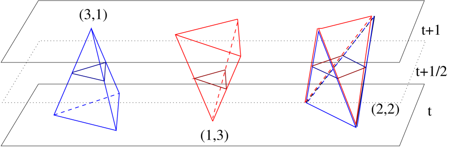
Figure 1: The three types of tetrahedral building blocks and their corresponding two-dimensional intersection patterns at $t=1/2$. By definition of the model, both the 3-1 and the 1-3 tetrahedra always occur in pairs.

The three types of building blocks are illustrated in Fig.1. Any three-dimensional “sandwich geometry” of height $\Delta t=1$ we construct from these building blocks can be uniquely described by the intersection pattern that results when the tetrahedra are sliced in half at time $t+1/2$ and the time-like triangles that are cut in the process are represented by one-dimensional links. We colour-code the links to distinguish whether they come from triangles with tip at $t$ (red links) or tip at $t+1$ (blue links). Our three building blocks can thus be represented by blue and red double-triangles and by squares with alternating blue-red sides. Topologically, the intersection graph is again a torus.

Figure 2: A regular triangular lattice serving as a “background geometry” at half-integer time $t+1/2$.

As already mentioned, we want to consider only amplitudes between flat two-tori. For the blue-red intersection picture this means that when the red links are simultaneously shrunk to zero length, what must remain is a regular tiling of a torus by (blue) triangles, where exactly six triangles meet at each vertex (and similarly at time $t+1$ when we shrink away the blue links). A systematic way of generating intersection patterns with this property is as follows. Take a rectangular strip of a regular triangular lattice of discrete width $l+w$ and height $m$, where the units are chosen in such a way that all vertices have integer coordinates (Fig.2). Let us for the moment take $l+w$ and $m$ to be even, $l=2l^{\prime}$, $w=2w^{\prime}$, $m=2m^{\prime}$, $l^{\prime},w^{\prime},m^{\prime}\in Z_{+}$, since this will make it possible to identify the opposite sides of this strip without any twists to create a compact two-torus. (In a more general model, one may also allow for twists in either of these directions.)

This regular lattice is to serve as a “background geometry” which we are going to tile with rhombic 2d building blocks so that no space is left blank. It is immediately clear that the intersections of the double-tetrahedra are blue and red rhombi. The squares that result from cutting the 2-2 tetrahedra will be “distorted” in this representation so that they can fit onto the triangular lattice. Since this can be done in two ways, we have a total of four rhombic tiles at our disposal (Fig.3a). It will be convenient for our purposes to adopt a dual notation where each rhombus is represented by a pair of crossing links. Each link connects two opposite edges of the rhombus and has the same colour, see Fig.3b. The rhombi can only be put onto the lattice if the colours of their edges (or their dual links) match pairwise at intersections.

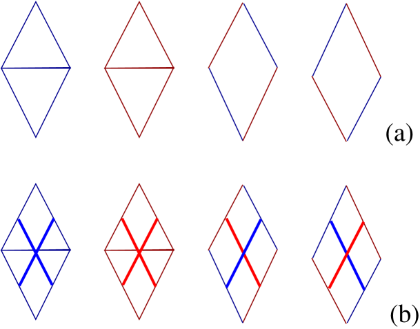
Figure 3: The four types of rhombic tiles (a), and their dual representation (b).

The beautiful feature of this representation is the fact that any tiling of the strip (which of course must be compatible with its periodic identifications) automatically leads to in- and out-geometries which are flat, connected tori. The easiest way of seeing this is by following dual links (or pieces of dual links) of a given colour around a closed loop, where the loop must be such that no more lines of the same colour branch off into the loop’s interior. Next, consider how this loop is represented in terms of triangles of the same colour which make up one of the adjacent spatial geometries. The pieces of straight coloured lines coming from the last two building blocks depicted in Fig.3b do not correspond to any triangles at all. By contrast, the first two rhombic tiles correspond to a couple of adjacent triangles each in the relevant spatial geometry at integer $t$. Since the rhombic tiles can be put onto the triangular “background lattice” at half-integer $t$ only with three possible orientations (see Fig.5 below), it is clear that any of the loops introduced above corresponds to a sequence of exactly six triangles.

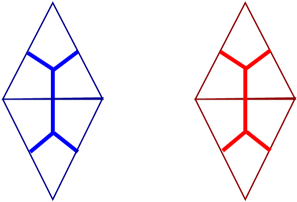
Figure 4: These tiles appear as blue and red double-triangles in spatial slices of integer $t$. Their trivalent dual graphs form part of regular hexagonal graphs representing flat two-geometries.

In fact, these two types of rhombi can more properly be represented by dual trivalent graphs which are dual to the individual triangles, as shown in Fig.4. It is then easy to see that each loop corresponds to a hexagon graph, with six “corners” of 120 degrees each, a property which has given the model its name. Translating this into a statement about the two-geometry, it means that there are six triangles meeting at each vertex, hence the geometry is everywhere flat. Thinking a little further along these lines, one can also convince oneself that it is not possible to obtain a flat triangulation of one colour that consists of two or more disconnected pieces.

3 Gravitational action and transfer matrix

The first step in constructing a path integral for our model is to determine which sandwich geometries $\Delta t=1$ can occur and to compute their contribution to the action. Following [5], this action can be written as a function of the total numbers $N_{31}$, $N_{13}$ and $N_{22}$ of tetrahedral building blocks occurring in the slice, namely,

$$S(\Delta t\!=\!1) =$$

$$(N_{31}+N_{13}) \Bigl{(}\pi k\sqrt{\alpha}-3k\ {\rm arcsinh}\ \frac{1}{\sqrt{3}\sqrt{4\alpha+1}}-3k\sqrt{\alpha}\arccos\frac{2\alpha+1}{4\alpha+1}-\frac{\lambda}{12}\sqrt{3\alpha+1}\Bigr{)}$$

$$+N_{22} \Bigl{(}2\pi k\sqrt{\alpha}+2k\ {\rm arcsinh}\ \frac{2\sqrt{2}\sqrt{2\alpha+1}}{4\alpha+1}-4k\sqrt{\alpha}\arccos\frac{-1}{4\alpha+1}-\frac{\lambda}{12}\sqrt{4\alpha+2}\Bigr{)},$$

where $\lambda$ and $k$ denote the bare cosmological and inverse Newton’s constants. The positive parameter $\alpha$ appearing in (LABEL:3dloract) describes the ratio between the squared lengths of the time-like and the space-like edges of the triangulation, $l_{\rm time}^{2}=-\alpha l_{\rm space}^{2}$. Since we will evaluate the state sums in the Euclidean sector of the theory, we need to Wick-rotate all of our Lorentzian discretized manifolds. As explained in detail in [4], this is achieved by continuing $\alpha$ through the complex lower half-plane to negative real values. Let us for simplicity choose the standard value $\alpha=-1$, so that all edges have the same length. This gives rise to the Euclidean action

$$S^{\rm eu}(\Delta t=1) = \!\!(N_{31}+N_{13})\Bigl{(}(-\frac{5}{2}\pi+6\arccos\frac{1}{3})k+\frac{1}{6\sqrt{2}}\lambda\Bigr{)}$$ (2)

$$+N_{22}\Bigl{(}(-2\pi+6\arccos\frac{1}{3})k+\frac{1}{6\sqrt{2}}\lambda\Bigr{)}$$

$$\equiv \!\!(N_{31}+N_{13})(-0.468k+0.118\lambda)+N_{22}(1.103k+0.118\lambda)$$

Obviously in our model the numbers of building blocks of type (3,1) and (1,3) are always even. Note also that the action (2) contains boundary terms (the discrete analogues of the usual spatial integrals over the extrinsic curvature) in order to make it additive under gluing of subsequent layers of $\Delta t=1$. The action without boundary contributions has the form

$$S^{\rm eu}_{\rm bulk}(\Delta t=1) = \!\!(N_{31}+N_{13})\Bigl{(}(-\pi+3\arccos\frac{1}{3})k+\frac{1}{6\sqrt{2}}\lambda\Bigr{)}$$ (3)

$$+N_{22}\Bigl{(}(-2\pi+4\arccos\frac{1}{3})k+\frac{1}{6\sqrt{2}}\lambda\Bigr{)}$$

$$\equiv \!\!(N_{31}+N_{13})(0.551k+0.118\lambda)+N_{22}(-1.359k+0.118\lambda).$$

The partition function or propagator for a single time-step after the Wick rotation is given by

$$G(g_{1},g_{2};\Delta t\!=\!1)=\sum_{T:g_{1}\rightarrow g_{2}}\frac{1}{C(T)}\mbox{e}^{-S^{\rm eu}(T)},$$ (4)

where the sum is over all possible sandwich geometries $T$ interpolating between the two spatial boundary geometries $g_{1}$ and $g_{2}$, and $C(T)$ is the order of the symmetry group of the triangulation $T$. As usual [4], expression (4) defines the transfer matrix $\hat{T}$ of the system with respect to the natural scalar product $\langle g_{1}|g_{2}\rangle=\frac{1}{C(g_{1})}\delta_{g_{1},g_{2}}$, via its matrix elements

$$\langle g_{2}|\hat{T}|g_{1}\rangle:=G(g_{1},g_{2};\Delta t\!=\!1).$$ (5)

4 The combinatorics of the intersections

In trying to characterize all possible intersection patterns that can occur (that is, all possible 3d sandwich geometries), it is convenient to break up the combinatorial problem into two steps. The first one is how to tile the triangular lattice with (identical) rhombi, and the second how to introduce a colouring on the resulting tilings (in the form of drawing chains of dual coloured links onto the rhombi).

Figure 5: There are three orientations in which a rhombus can be put onto the triangular background lattice.

A rhombus can be put onto the lattice with three different orientations, which we call A, B and C. This is illustrated in Fig.5, where the centres of the rhombi are indicated by small circles. Fig.6 shows a complete periodic tiling of a strip with $(l+w,m)=(12,4)$. (Opposite sides of this strip are to be identified.) What should be noted here is that the number of A-blocks as well as the combined number of B- and C-blocks per horizontal row is conserved as one advances in steps in the $m$-direction. Starting at some B- or C-block in row 1, one can therefore follow a “path” in vertical direction made up of some sequence of B- and C-rhombi until one reaches the upper end of the strip (shaded region in Fig.6).

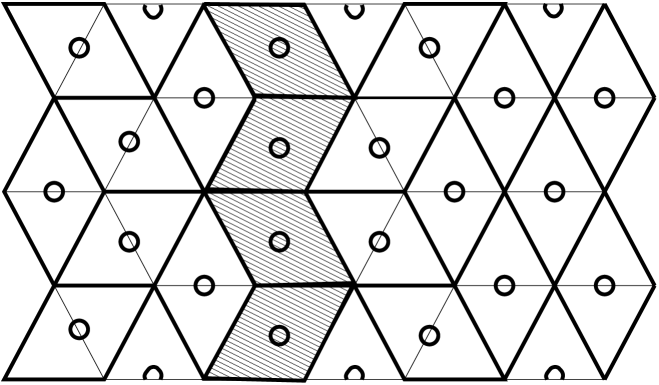
Figure 6: A tiling with A-, B- and C-rhombi (as usual, opposite sides of the strip are to be identified). The shaded region is a B-C-path of winding number 1 in the vertical direction.

At this stage we will for simplicity impose a further restriction on the allowed patterns of rhombi, namely, that all B-C-paths should have winding number zero in the $l$-direction and winding number one in the $m$-direction. (This does not seem to impose serious restrictions on the in- and outgoing two-geometries, c.f Secs. 6, 7, but is a condition that could be relaxed, should this turn out to be convenient.) That is, following such a path between the lower and upper end of a strip, it should contain an equal number of B- and C-rhombi, so that it closes on itself upon identification of the lower and upper ends of the strip. A configuration which violates this restriction but is nevertheless periodic is shown in Fig.7.

Figure 7: An example of a forbidden tiling.

By shrinking all B-C-paths to zero width, one obtains a regular tiling of only A-rhombi (Fig.8, left). This reduced lattice can be thought of as a sublattice of the original strip in the sense that the chains of its dual A-links close onto themselves. If the number of B-C-paths was $w/2$, the reduced lattice will have width $l$ and height $m$. Note also that these chains take the very simple form of straight diagonal left- or right-moving lines. A configuration of dual A-lines is most easily represented as a tilted square lattice (Fig.8, right). The intersection points of the dual left- and right-moving lines will then have $l$-coordinate 0,2,4,6,…in the odd rows and 1,3,5,… in the even rows.

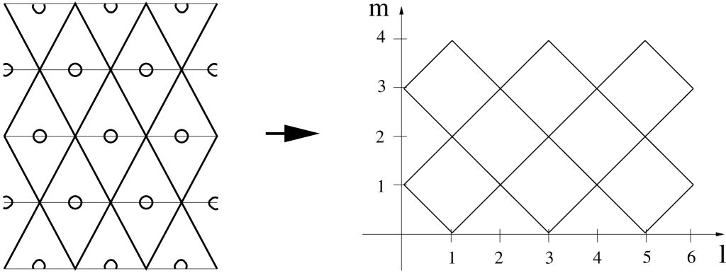
Figure 8: The regular tiling with A-rhombi obtained by deleting the B- and C-rhombi from Fig.6 (left), and the corresponding dual tilted square lattice (right).

As will become apparent in due course, working out the possible colour assignments for such dual A-lattices is an important part of the combinatorics of the model. They are quite easy to enumerate. By assumption, any colouring of the dual chains has to respect periodicity in both $l$- and $m$-directions. The easiest way to obtain a consistent colouring is therefore as follows. Start at some (dual) vertex $v$ at $m=0$ and colour the, say, left-moving A-line passing through $v$ while following it around the lattice (keeping in mind the periodic identifications of the strip), until getting back to the original vertex. Using such a procedure, it is straightforward to see that the number of possible colourings for the entire configuration of A-lines depends on the integer $d$, the greatest common divisor of $l/2$ and $m/2$. (For example, the lattice depicted in Fig. 8 has $l=6$, $m=4$ and therefore $d=1$.) Picking an arbitrary vertex $v$ at $m=0$ as origin, the colours of the left- and right-moving A-lines emanating from the first $d$ vertices to its right (including $v$) may be chosen arbitrarily, with the remainder determined by periodicity.

To count intersections of a certain type between the right- and left-moving A-lines (important for determining the action) it suffices to look at a fundamental diamond-shaped region of $d\times d$ vertices – this region will then be repeated $lm/2d^{2}$ times throughout the lattice.

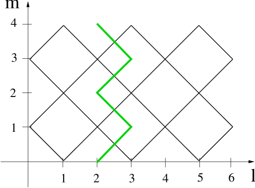
Figure 9: The B-C-strands may be reintroduced by drawing paths onto the regular dual A-strip. In the figure, we have drawn the path corresponding to the shaded area in Fig.6.

We may now reintroduce the B-C-strands into this picture by drawing chains of links whose vertices in every row lie exactly in between the dual A-vertices. Starting from the initial row $m=0$, we can again follow paths of dual B- or C-links by making at every vertex a choice of moving diagonally up to the left or to the right (Fig.9). More than one dual B-C-chain can pass through any one vertex, and neighbouring chains are allowed to share one or more links, but not to cross, so that their relative position along the $l$-direction is preserved as we advance in $m$. (Obviously, to obtain configurations of the type depicted in Fig.6, each of these paths must be “blown up” in the horizontal direction to width 2.)

The combinatorics of the B-C-chains can be mapped onto a model of so-called vicious walkers (which are not allowed to touch) with fixed initial and final points, by inserting columns of width 2 between every pair of adjacent B-C-chains. Various versions of vicious-walker models, differing in their boundary conditions for the paths and the underlying lattices, have been investigated in the literature. The most common choice is that of free boundary conditions in the $l$-direction, i.e. a lattice of effectively infinite width. The initial points of the walkers at $m=0$ are usually located at a minimal mutual distance $\Delta l=2$ near the origin, for example, at $l$-coordinate 0, 2, 4, … , $w-2$, and the final points at $m_{\rm max}$ are either chosen freely or again grouped together at some point $(l_{0},m_{\rm max})$ with $l$-coordinates $l_{0}$, $l_{0}+2$, $l_{0}+4$, … , $l_{0}+w-2$ (see, for example, [19, 20, 21] and references therein). An exception is the treatment by Forrester [22], who uses periodic boundary conditions in the $l$-direction and walkers with equally (but not necessarily minimally) spaced initial and final positions.

The case relevant for our 3d gravity model is that of periodic boundary conditions in both the $l$- and $m$-direction, and the combinatorial problem can be phrased as follows: Given three even integers $l$, $m$ and $w$, how many ways are there of drawing $w/2$ indistinguishable vicious-walker paths with winding numbers $(0,1)$ onto a tilted square lattice of width $l+w$ and height $m$? The tilted square lattice is dual to similar lattices depicted in Figs.8, 9, i.e. it has vertices on the horizontal axis at even parameter values $0,2,4,\dots,l+w-2$ and vertices on the vertical axis at values $0,2,4,\dots,m$. Fig.10 shows a typical configuration of vicious walkers for $(l,m,w)=(10,10,6)$. The vertical boundaries of this lattice are identified periodically as indicated in the figure, so that $l+w\equiv 0$. Each vicious-walker path starts on the lower horizontal axis at some point $(l,0)$ and ends after $m$ steps on the upper horizontal boundary at the point $(l,m)$, i.e. at the point with the same horizontal coordinate.

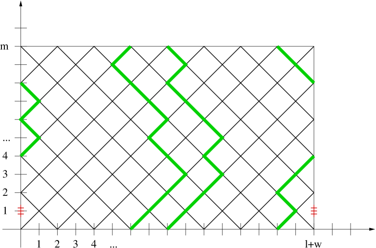
Figure 10: A configuration of three vicious walkers, corresponding to $(l,m,w)=(10,10,6)$.

This situation can be viewed as a special case of that of a single random walker in an alcove of the affine Weyl group of type $\tilde{A}_{w/2-1}$ [23]. The reflections of the path at the walls of the Weyl chamber correspond in this case to the collision points of $w/2$ random walkers that move on a one-dimensional circle. The ensemble of walkers takes simultaneously steps of unit length along the circle, either to the right or the left. Mapping these onto diagonal upward steps on a tilted square lattice and requiring identical initial and final points for each walker on the circle leads exactly to a situation as depicted in Fig. 10. Following [24, 23], the number of non-intersecting path configurations for $w/2$ walkers with initial and endpoints $\vec{\lambda}=(\lambda_{1},\lambda_{2},\dots,\lambda_{w/2})$, $\lambda_{i}\in\{0,2,4,\dots,l+w-2\}$, ordered along the circle so that $\lambda_{1}<\lambda_{2}<\dots<\lambda_{w/2}$, is given by

$$b(\vec{\lambda},m,l,w)=\sum_{\vec{t},\;\sum t_{i}=0}\,\det_{\frac{w}{2}\times\frac{w}{2}}\,\left|\Biggl{(}{m\atop(m/2)+\frac{l+w}{2}\,t_{i}+\lambda_{j}-\lambda_{i}}\Biggr{)}\right|,$$ (6)

where $\vec{t}$ is a $w/2$-tupel of integers. Note that because of the properties of the binomial coefficients, only a finite number of terms in the sum over $\vec{t}$ is non-vanishing. The presence of the determinants has to do with the fact that although all possible path configurations appear in (6), the contributions from configurations with touching or intersecting walkers cancel appropriately by virtue of the alternating signs in the determinantal sum, in such a way that only the non-intersecting ones are left over. The largest term that can appear in any of the determinants on the right-hand side of (6) is always the product of the elements on the diagonal, namely,

$$\Biggl{(}{m\atop m/2}\Biggr{)}^{\frac{w}{2}},$$ (7)

corresponding to the independent product of $w/2$ periodic, free random walks consisting of $m$ steps.

5 Adding colour and estimating the entropy

The hexagon model possesses a feature that will simplify the (asymptotic) analysis of the propagator. This has to do with the fact that each intersection pattern characterizing a sandwich geometry can be brought to a standard form by using a sequence of moves which affect neither the in- and outgoing 2d torus geometries nor the value of the action (2).

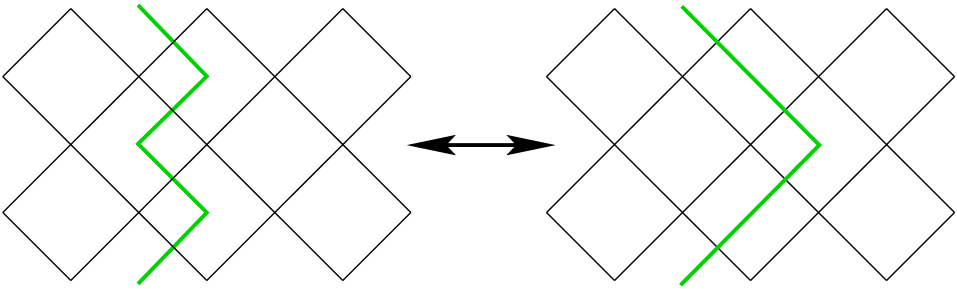
Figure 11: The effect of a wedge flip on a B-C-path drawn on the dual A-lattice.

The basic idea is to move all B-C-paths to the far left of the strip. The elementary move necessary to achieve this is the flip of a left-right wedge (an adjacent pair of a dual B- and C-link) to a right-left wedge or vice versa (Fig.11). Since any B-C-chain has by assumption an equal number of B- and C-links, it can be moved to the left of the strip (where it assumes the form of a zigzag path) by a finite sequence of such moves. In the process, it will cross (pieces of) A-chains, but not other B-C-chains. A typical final result after applying this procedure to all B-C-chains of an intersection pattern is illustrated in Fig.12.

Figure 12: A rhombic tiling of standard form.

Figure 13: The rearrangement of the rhombi making up a fundamental hexagon region during a wedge flip and of the associated dual links or lines.

In order to understand which consequences the wedge flip has for the geometry, let us analyze which action it translates to on the unreduced rhombic tiling. The region on the original triangular lattice which is affected by the wedge flip is confined to a set of six triangles forming a single hexagon, with six dual links emerging from the sides of the hexagon. There are two ways of tiling this fundamental hexagon by three rhombi. In both cases, there is a piece of B-C chain entering at the bottom of the hexagon and coming out at the top, a piece of a right-moving A-chain entering at the bottom left and exiting at the top right side of the hexagon and a piece of left-moving A-chain entering at the bottom right and coming out at the top left. The wedge flip changes the tiling of the fundamental hexagon and the intersection patterns of the dual chains in the interior of the hexagon, without altering the dual links emanating from it (Fig.13).

To determine the effect on the geometry, one has to consider all possible colourings of the chains passing through the hexagon and how the wedge flip affects the blue and red dual link patterns. The first case is that where all lines have the same colour, say, blue, which implies that the hexagon represents a gluing of six 3-1 tetrahedra. The wedge flip only alters the way in which we mentally divide this set of six tetrahedra into three double-tetrahedra. Obviously this move does not in any way affect the three-geometry, and the geometries before and after the move should not be counted as distinct. However, for all other colour choices (there is a total of six) the three-geometry genuinely changes. As one can easily verify, the wedge flip in all of these cases corresponds to pulling a piece of a red chain (without vertices) across a blue-blue intersection or the other way round. This means that the individual red and blue dual graphs are squeezed and stretched in the process, but remain otherwise completely unaffected, and hence will correspond to the same two-geometries.

Since moreover the number of building blocks of a certain type (3-1, 1-3 or 2-2) does not change under a flip move, we have proved our original assertion that the wedge flip leaves all two- and three-volumes (and hence the action) as well as the Teichmüller parameters of the two-geometries invariant. We recognize here a simplified feature of the hexagon model, compared with the most general dynamically triangulated 3d gravity model [4, 5], even if we restricted its integer-$t$ slices to be flat tori. Namely, although the toroidal two-geometries forming the spatial boundaries of a space-time sandwich $\Delta t=1$ by no means fix the three-geometry inbetween the two slices, they determine essentially uniquely the value of the sandwich action $S(\Delta t=1)$. In other words, there is a large number of interpolating space-time geometries for given, fixed boundaries, but they all contribute with the same weight e^iS. A main task in solving the model is therefore the computation of the number of distinct interpolating 3-geometries between two adjacent flat two-tori.

Before we can give a precise definition of this combinatorial problem, we still need to specify how we are going to parametrize the colouring of the rhombic intersection pattern. Since we have already shown that any intersection pattern characterizing a three-geometry can be brought to standard form without affecting the individual red and blue torus geometries, we may without loss of generality think of the latter as subgraphs of this standard form. Using the notation introduced above, we will label the uncoloured standard form by three even integers $(w,l,m)$, where $w/2$ is the number of zigzag B-C-chains on the left (whose individual height is $m$) and $(l,m)$ is the size of the regular lattice of A-rhombi on the right.

Let us now introduce a colouring by drawing closed dual lines onto this standard form, thereby producing a coloured standard form $\cal S$. There are obviously $w/2$ independent vertical lines that can be drawn onto the B-C-columns. We will split them into $w_{1}/2$ blue lines and $w_{2}/2\equiv(w-w_{1})/2$ red lines. It is clear that the order in which we colour these strands will affect the three-geometry, but not the individual two-geometries or the action. This results in a multiplicity $\Bigl{(}{w\atop w_{1}}\Bigr{)}$ for given in- and out-states, counting the number of possible orderings of blue and red vertical dual lines.

We turn next to the colouring of the remaining dual lines, i.e. those that traverse the B-C-chains horizontally and the A-rhombi diagonally. The choice is restricted by the fact that the number of such lines which are closed (and therefore can be coloured independently) is exactly $d$ for the right-moving and $d$ for the left-moving lines. We will denote the numbers of blue right-moving and left-moving dual lines by $a_{r}$ and $a_{l}$, and those of the corresponding red lines by $b_{r}\equiv d-a_{r}$ and $b_{l}\equiv d-a_{l}$. As before, the relative ordering of the blue and red lines in either direction leads in general to different three-geometries, but leaves the two-geometries and the action unchanged, thus contributing a factor $\Bigl{(}{d\atop a_{r}}\Bigr{)}\Bigl{(}{d\atop a_{l}}\Bigr{)}$ to the number of interpolating states.

Putting all of these observations together, we can now rewrite the one-step propagator (4) in a more explicit form. Using the essentially unique association $(g_{1},g_{2})\leftrightarrow(l,m,w_{1},w_{2},a_{l},a_{r})$ (c.f. Sec. 6 and Appendix 1), $G$ now takes the form

$$G(g_{1},g_{2},\Delta t\!=\!1)=\sum_{\cal O}\frac{1}{C({\cal S})}\tilde{M}({\cal S})\Bigl{(}{w_{1}+w_{2}\atop w_{1}}\Bigr{)}\Bigl{(}{d\atop a_{r}}\Bigr{)}\Bigl{(}{d\atop a_{l}}\Bigr{)}\;\mbox{e}^{-S^{\rm eu}({\cal S})}.$$ (8)

The number $\tilde{M}({\cal S})$ counts the distinct strip configurations that can be obtained by applying elementary wedge flips to the coloured standard form ${\cal S}$, uniquely described by the six parameters $(l,m,w_{1},w_{2},a_{l},a_{r})$, and the relative order $\cal O$ of their dual coloured lines. (We are regarding configurations that differ by overall translations in the $l$- and $m$-direction as equivalent. At any rate, this choice does not affect the remainder of our discussion.)

In view of the discussion in Sec. 1, we are interested in the continuum behaviour of (8), and in particular how the entropy contributions compete with the kinematical action $S^{\rm eu}$ to result in an effective (continuum) action. The combinatorial part $\tilde{M}({\cal S})$ of (8) is very similar to that of the uncoloured problem described in connection with Fig.10, but the colour-dependence does now enter in a slightly subtle way. This again has to do with the slight overcounting present in our model (the subdivision of fundamental hexagon regions of one colour) which implies that not all vicious-walker configurations will correspond to distinct three-geometries. How often this occurs depends on both the boundary geometries $g_{i}$ and the relative order $\cal O$ of coloured lines of an individual sandwich geometry. It is clear that the overcounting will be most pronounced when the intersection pattern has very many dual links of one colour and very few of the other, because this will result in many local fundamental hexagon regions of one colour which are insensitive to wedge flips, cf. Fig. 13.

Let us proceed on the assumption that – at least to leading order – the scaling behaviour of the entropy will not be affected by this overcounting. This is in part justified by the numerical investigations of [5], where we found that in the continuum limit, neighbouring spatial slices are strongly coupled, in the sense of having a similar total volume. Under this assumption, we can drop the sum over $\cal O$ in (8), and substitute the combinatorial factor by $\tilde{M}=M$, where

$$M(m,l,w):=\sum_{\vec{\lambda}}b(\vec{\lambda},m,l,w)$$ (9)

is the sum over all ordered $w/2$-tupels of initial conditions $\vec{\lambda}$ for a set of random walkers. We would like to establish the behaviour of $M$ in the limit as $(m,l,w)$ simultaneously become large. This is not completely straightforward, since according to (6) each $b$ is a sum of terms that can be both positive and negative.

For the purposes of this paper we will concentrate on establishing the leading divergent behaviour of $M$; we hope to return to the full analytic solution of the model in the near future. Is it the case that the leading behaviour is given by exp($c$ spatial volume), for some positive constant $c$? As explained earlier, this is needed for obtaining truly extended geometries in the continuum limit and a necessary prerequisite for a conformal-factor cancellation. The continuum limit that has been considered in most of the literature on vicious walkers is that in which both the width and the length of the lattice become large, but not the number of walkers. In this case one typically finds for the number $\cal N$ of walker configurations

$${\cal N}=2^{{\rm number\;of\;walkers\;}\times{\rm number\;of\;steps}}\times\,{\rm(subleading\;terms)}.$$ (10)

This is precisely the type of scaling behaviour we are looking for, but not the physical situation we are interested in, since the paths here are “diluted” (even though their initial and final points may lie close together).

A scenario of more immediate interest to us is again that considered by Forrester we already cited earlier [22], who treats the case of $N$ equally spaced walkers on a lattice of width $\mu$ with initial conditions $\lambda_{i}=i\nu$, $i=1,...,N$, so that $\nu=\mu/N$ is the average distance between the walkers’ paths. However, it should be noted that his class of path configurations is larger than ours: although he also considers periodic boundary conditions in the $m$-direction, an individual walker’s path is not required to close on itself after $m$ steps, but may wind around the lattice several times before doing so. The resulting closed paths will in general have $(l,m)$-winding numbers different from (0,1) (an example is shown in Fig. 7) which by definition we have excluded from our current model. The evaluation of the combinatorics of this more general case turns out to be easier because it involves determinants of cyclic matrices, which can be simplified. For even $m,\nu$ and odd $N$ the number of vicious-walker configurations is given by [22]

$${\cal N}^{F}(N,m,\nu)=\prod_{p=0}^{N-1}\,\frac{2}{\nu}\,\sum_{b=0}^{\nu/2-1}2^{m}\cos^{m}(\frac{2\pi}{\nu}(\frac{p}{N}+b)).$$ (11)

However, it is easy to see that the overcounting involved in (11) does not alter the leading behaviour for large $N$ and $m$ compared to our more restricted case. Namely, we can divide the path configurations counted by (11) into different sectors, depending on the lateral displacement $\Delta=\lambda_{final}-\lambda_{initial}$ of the initial and final point of each walker. We have $\Delta_{max}=\pm m$, with the largest contribution to ${\cal N}^{F}$ coming from configurations with $\Delta=0$ (corresponding exactly to the path configurations with winding number 1 we are counting in the hexagon model). The asymptotics of (11) is much easier to handle, since the right-hand side is a product of sums over positive terms. Assuming an appropriate monotonic behaviour of ${\cal N}^{F}$, it follows from the results in Appendix 2 that the leading divergence for $N,m\rightarrow\infty$ and fixed $\nu>2$ is given by

$${\cal N}^{F}(N,m,\nu)\sim c(\nu)^{mN},\;\;\;2\ \cos(\frac{\pi}{\nu})\leq c(\nu)\leq 2.$$ (12)

Coming back to the combinatorics of the function $M$, note that for a given lattice width and number of walkers there are $\Bigl{(}{(l+w)/2-1\atop w/2}\Bigr{)}$ terms contributing to the sum (9), corresponding to all possible initial conditions for the walkers. Since this number grows at most exponentially in length (as opposed to volume), the leading exponential behaviour will coincide with that of the largest term in the sum, which is roughly speaking that of the configuration(s) where the walkers are maximally distributed (i.e. spaced out in the $m$-direction) over the available space and therefore get least in the way of each other. We can identify their average distance with the spacing $\nu$ appearing in Forrester’s formulas. (Strictly speaking, $\nu$ is of course an (even) integer, but we do not expect this to play a role in the continuum limit.) We may therefore conclude that for an average spacing $\nu\equiv(l+w)/w$, and in the limit as $m,l,w\rightarrow\infty$, the number of vicious-walker configurations behaves to leading order like

$$M(m,l,w)\sim c(\nu)^{mw/2}\times\;{\rm(subleading\;terms)},$$ (13)

where $c(\nu)$ is a constant of order 2, which appeared in (12). This shows that the hexagon model of three-dimensional quantum gravity has indeed enough entropy, compared with more restricted cosmological models that were studied previously.

6 Teichmüller parameters for triangulated tori

Our next task will be to relate the parameters $(l,m,w_{1},w_{2},a_{l},a_{r})$, introduced in the previous section to label a standard coloured three-geometry, to the variables describing the two spatial boundaries of that geometry. In this way we will achieve a clean separation of the geometric in- and out-data $g_{1}$ and $g_{2}$ appearing as arguments of the amplitude $G$, and make contact with the standard parametrization of two-dimensional flat tori.

It is a well-known fact that in the continuum any flat torus geometry $g$ can be characterized by three numbers $(v,\tau_{1},\tau_{2})$, where $v$ is the two-volume (in our case proportional to the number of triangles that make up the torus) and the $\tau_{j}$ are the two real Teichmüller parameters. We would like to compute the geometric data $(v^{(i)},\tau_{1}^{(i)},\tau_{2}^{(i)})$, $i=1,2$, for the individual two-tori from the parameters $(l,m,w_{1},w_{2},a_{l},a_{r})$.

Recall that the numbers of blue, red and blue-red rhombi at time $t+1/2$ is given by $N_{31}/2$, $N_{13}/2$ and $N_{22}$ respectively. The first two numbers give us directly the discrete two-volumes of the spatial slices at times $t$ and $t+1$, namely, $v^{(1)}=N_{31}$ and $v^{(2)}=N_{13}$. (In order to obtain the volume in terms of the lattice spacing $a$, one needs to multiply with the volume of a Euclidean triangle, which is $a^{2}\sqrt{3}/4$.) Taking into account the considerations of Sec. 4 on the division of the A-lattice into fundamental regions, one derives for these numbers the expressions

$$N_{31} = w_{1}\frac{m}{2d}(a_{r}+a_{l})+\frac{lm}{d^{2}}a_{r}a_{l},$$

$$N_{13} = w_{2}\frac{m}{2d}(b_{r}+b_{l})+\frac{lm}{d^{2}}b_{r}b_{l},$$

$$N_{22} = \frac{m}{4d}(w_{1}(b_{r}+b_{l})+w_{2}(a_{r}+a_{l}))+\frac{lm}{2d^{2}}(a_{r}b_{l}+a_{l}b_{r}).$$ (14)

In order to determine the Teichmüller parameters for the tori, we will identify for each colour (blue or red) a pair of oriented, closed geodesics, i.e. straight lines of minimal length on the corresponding torus at time $t$ or $t+1$. (Note that these do not have to coincide with any triangle edges.) Each pair consists of a circle with winding number $(1,0)$ and one with winding number $(0,1)$ when viewed as curves on the intersection pattern at $t+1/2$ (the two winding numbers refer to the horizontal $l,w$-direction and the vertical $m$-direction). The winding numbers of closed curves in the spatial two-geometries can therefore be thought of as “inherited” from the three-dimensional geometry. These curves are clearly unique up to two-dimensional translations (if we think of the flat tori at integer time $t$ as being rolled out into the two-dimensional plane). For a given colour, their lengths and their relative intersection angle are translation-invariant, and in one-to-one correspondence with the torus parameters $(v,\tau_{1},\tau_{2})$.

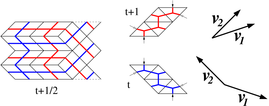
Figure 14: An intersection pattern at time $t+1/2$ gives rise to a blue triangulation at time $t$ and a red triangulation at time $t+1$. We also show the two vectors ${\cal V}_{1}$ and ${\cal V}_{2}$ representing the closed geodesics of winding number (1,0) and (0,1) for both of these geometries.

Let us look at a simple example in order to illustrate this procedure. Fig.14 shows on the left a coloured intersection pattern in standard form representing a sandwich geometry, and consisting of 12 rhombi. It gives rise to two spatial boundary geometries, both of them flat tori with four triangles each. They have been cut open and are represented by two parallelograms in the plane, where the small black and white arrows indicate how their opposite sides are to be identified pairwise. Each of these two-geometries has oriented geodesics with winding number (1,0) and (0,1) respectively. They can be represented by a pair of vectors $({\cal V}_{1},{\cal V}_{2})$ drawn onto the parallelogram. For ease of representation, the vectors are depicted on the right with their correct lengths and orientations, and with a common origin.

It remains to compute the lengths and angles of these vectors from the data $(l,m,w_{1},w_{2},a_{r},a_{l},b_{r},b_{l})$ characterizing the coloured intersection pattern in standard form. Representing the blue closed geodesic with winding number $(1,0)$ at time $t$ as a two-dimensional vector ${\cal V}_{1}^{(1)}$ and the blue closed geodesic with winding number $(0,1)$ as a second vector ${\cal V}_{2}^{(1)}$, one finds in terms of the discrete units inherited from the $(l,m)$-coordinate system at $t+1/2$

$${\cal V}_{1}^{(1)} = \Bigl{(}\frac{l}{2d}(a_{l}+a_{r})+w_{1},\frac{l}{2d}(a_{l}-a_{r})\Bigr{)},$$

$${\cal V}_{2}^{(1)} = \Bigl{(}\frac{m}{2d}(a_{l}-a_{r}),\frac{m}{2d}(a_{l}+a_{r})\Bigr{)}.$$ (15)

Translating this into absolute units, one finds

$${\cal V}_{1}^{\prime(1)} = \Bigl{(}\frac{l}{4d}(a_{l}+a_{r})+\frac{w_{1}}{2},\frac{\sqrt{3}l}{4d}(a_{l}-a_{r})\Bigr{)}a,$$

$${\cal V}_{2}^{\prime(1)} = \Bigl{(}\frac{m}{4d}(a_{l}-a_{r}),\frac{\sqrt{3}m}{4d}(a_{l}+a_{r})\Bigr{)}a,$$ (16)

where $a$ again denotes the lattice spacing. The two vectors ${\cal V}_{1}^{\prime(2)}$, ${\cal V}_{2}^{\prime(2)}$ characterizing the red triangulation at time $t+1$ are obtained by substituting $a_{l},a_{r},w_{1}$ in (16) by $b_{l},b_{r},w_{2}$. Note that the relations (16) imply the inequalities

$${\cal V}_{1,1}^{\prime(i)}\geq 0,\;\;{\cal V}_{2,2}^{\prime(i)}\geq 0,\;\;{\cal V}_{1,1}^{\prime(i)}\geq|{\cal V}_{1,2}^{\prime(i)}|,\;\;{\cal V}_{2,2}^{\prime(i)}\geq|{\cal V}_{2,1}^{\prime(i)}|.$$ (17)

As is shown in Appendix 1, the coordinate transformation between the six variables $(l,m,w_{1},w_{2},a_{l}/d,a_{r}/d)$ and the components of the vectors ${\cal V}_{j}^{\prime(i)}$, subject to the constraints

$${\cal V}_{1,2}^{\prime(2)}=-{\cal V}_{1,2}^{\prime(1)},\;\;{\cal V}_{2,1}^{\prime(2)}=-{\cal V}_{2,1}^{\prime(1)},$$ (18)

is one-to-one.

Figure 15: Standard representation of a flat torus with Teichmüller parameter $\tau=\tau_{1}+i\tau_{2}$ as a parallelogram in the complex $\tau$-plane.

Up to a common rotation and a global rescaling, each pair of vectors $({\cal V}_{1}^{\prime(i)},{\cal V}_{2}^{\prime(i)})$ can be identified with the vectors spanning the parallelogram in the standard representation of a flat torus with normalized area in the complex $\tau^{(i)}$-plane ($\tau^{(i)}=\tau_{1}^{(i)}+i\tau_{2}^{(i)}$), Fig.15. It is straightforward to compute the SO(2)-rotation

$$\Bigl{(}\matrix{\;\;\cos\phi^{(i)}&\sin\phi^{(i)}\cr-\sin\phi^{(i)}&\cos\phi^{(i)}}\Bigr{)}$$ (19)

which aligns the vector ${\cal V}_{1}^{\prime(i)}$ with the $\tau_{1}^{(i)}$-axis. One finds

$$\cos\phi^{(1)}=\frac{a}{L^{(1)}}(\frac{l}{4d}(a_{l}+a_{r})+\frac{w_{1}}{2}),\hskip 28.45274pt\sin\phi^{(1)}=\frac{a}{L^{(1)}}\frac{\sqrt{3}l}{4d}(a_{l}-a_{r}),$$ (20)

where $L^{(1)}$ denotes the length of the vector ${\cal V}_{1}^{\prime(1)}$,

$$L^{(1)}:=||{\cal V}_{1}^{\prime(1)}||=\sqrt{\Bigl{(}\frac{l}{4d}(a_{l}+a_{r})+\frac{w_{1}}{2}\Bigr{)}^{2}+\Bigl{(}\frac{\sqrt{3}l}{4d}(a_{l}-a_{r})\Bigr{)}^{2}}\,a.$$ (21)

The corresponding expressions for $\cos\phi^{(2)}$, $\sin\phi^{(2)}$, $L^{(2)}$ are obtained by substituting $(a_{l},a_{r},w_{1})\mapsto(b_{l},b_{r},w_{2})$.

We still have to rescale all lengths by a factor $1/L^{(1)}$ so that the rotated vector ${\cal V}_{1}^{\prime(1)}$ assumes length 1. Applying then both the rotation (19), (20) and this rescaling to the vector ${\cal V}_{2}^{\prime(1)}$, we can read off directly the dimensionless Teichmüller parameters $\tau_{i}^{(1)}$. Collecting the geometric data describing uniquely the blue torus at time $t$, we have finally

$$v^{(1)} = \Bigl{(}a_{l}a_{r}\frac{lm}{d^{2}}+(a_{l}+a_{r})\frac{mw_{1}}{2d}\Bigr{)},$$

$$\tau_{1}^{(1)} = \frac{m}{4d(L^{(1)})^{2}}\Bigl{(}(a_{l}^{2}-a_{r}^{2})\frac{l}{d}+(a_{l}-a_{r})\frac{w_{1}}{2}\Bigr{)}a^{2},$$

$$\tau_{2}^{(1)} = \frac{m}{4d(L^{(1)})^{2}}\Bigl{(}a_{l}a_{r}\frac{\sqrt{3}l}{d}+(a_{l}+a_{r})\frac{\sqrt{3}w_{1}}{2}\Bigr{)}a^{2}\equiv\frac{\sqrt{3}}{4}\frac{a^{2}}{(L^{(1)})^{2}}v^{(1)}.$$ (22)

The map between the independent vector components ${\cal V}_{i,j}^{\prime(k)}$ (or, equivalently, the sandwich variables $(l,m,w_{1},w_{2},a_{l}/d,a_{r}/d)$) and the $(v^{(k)},\tau^{(k)})$ is in general two-to-one (see Appendix 1).

One may also wish to reexpress the action in terms of these torus parameters. Because the transformation to these parameters is not bijective, this can only be done modulo a sign ambiguity. One first writes the counting variables $N_{ij}$ as functions of the two-vectors ${\cal V}^{\prime(k)}$ and then in turn expresses the latter as functions of the torus parameters. Details of these calculations can again be found in Appendix 1. The explicit form for the sandwich action $S^{\rm eu}({\cal S})=S^{\rm eu}(v^{(1)},\tau^{(1)},v^{(2)},\tau^{(2)})$ is given by (2), with

$$N_{31} \!\!=\!\! v^{(1)}$$

$$N_{13} \!\!=\!\! v^{(2)}$$

$$N_{22} \!\!=\!\! \frac{1}{2}\frac{1}{(\tau_{1}^{(1)}+\tau_{1}^{(2)})^{2}+(\tau_{2}^{(1)}-\tau_{2}^{(2)})^{2}}\Biggl{(}-2(\tau_{1}^{(1)}\tau_{2}^{(2)}+\tau_{1}^{(2)}\tau_{2}^{(1)})\Bigl{(}v^{(1)}\frac{\tau_{1}^{(1)}}{\tau_{2}^{(1)}}+v^{(2)}\frac{\tau_{1}^{(2)}}{\tau_{2}^{(2)}}\Bigr{)}$$ (23)

$$- \Omega\;\Bigl{(}(\tau_{1}^{(1)})^{2}-(\tau_{1}^{(2)})^{2}+(\tau_{2}^{(1)})^{2}-(\tau_{2}^{(2)})^{2}\Bigr{)}\Biggr{)}.$$

The function

$$\Omega=({\cal V}_{1,1}^{\prime(1)}{\cal V}_{2,2}^{\prime(2)}-{\cal V}_{2,2}^{\prime(1)}{\cal V}_{1,1}^{\prime(2)})\frac{4}{a^{2}\sqrt{3}}$$ (24)

can be expressed in terms of the $(v^{(k)},\tau^{(k)})$ only up to a sign, namely, as the positive and negative square-root of

$$\Omega^{2}=\frac{v^{(1)}v^{(2)}}{\tau_{2}^{(1)}\tau_{2}^{(2)}}\Bigl{(}(\tau_{1}^{(1)}+\tau_{1}^{(2)})^{2}+(\tau_{2}^{(1)}-\tau_{2}^{(2)})^{2}\Bigr{)}-\Bigl{(}v^{(1)}\frac{\tau_{1}^{(1)}}{\tau_{2}^{(1)}}+v^{(2)}\frac{\tau_{1}^{(2)}}{\tau_{2}^{(2)}}\Bigr{)}^{2}.$$ (25)

The resulting action has a feature that may at first seem puzzling. Let us think of the exponentiated action for fixed boundary geometries as a matrix element (c.f. equation (5)),

$${\rm e}^{-S^{\rm eu}(v^{(1)},\tau^{(1)},v^{(2)},\tau^{(2)})}=:\langle v^{(2)},\tau^{(2)}|\hat{t}|v^{(1)},\tau^{(1)}\rangle.$$ (26)

Usually this kinematical “transfer matrix” can be written as $\hat{t}={\rm e}^{-a\hat{h}}={\bf 1}-a\hat{h}+O(a^{2})$, where $\hat{h}$ denotes the discrete, kinematical Hamilton operator of the system, and where we have reintroduced the discrete unit $\Delta t=a$ for a single time step.

For such an expansion to exist, in the limit of small $\Delta t$ the configuration variables at a neighbouring spatial slice should always be expressible as $v(t+a)\simeq v(t)+a\dot{v}$, $\tau(t+a)\simeq\tau(t)+a\dot{\tau}$. However, looking at the explicit formulas for $\tau_{1}^{(1)}$ and $\tau_{1}^{(2)}$ (representing the variable $\tau_{1}$ at two adjacent spatial slices) as functions of $a_{l}$ and $a_{r}$, one sees that they always have opposite signs. It is therefore kinematically impossible to set them equal unless they both vanish (or, equivalently, $a_{l}=a_{r}$). This can be traced back to the fact that a natural “pairing” between two neighbouring spatial geometries occurs in our construction by putting their two graphs together in an intersection pattern. As can be seen from the elementary example depicted in Fig.14, the natural “dual” of a particular blue graph is given not by the graph itself, but by its reflection, where the relative orientation of the two coordinate axes has been reversed. In terms of the Teichmüller parameters (since by definition we always keep $\tau_{2}\geq 0$) this amounts to a map $R:\tau_{1}\mapsto-\tau_{1}$, with a lowest-order expansion $\hat{t}=R+O(a)$ for the matrix $\hat{t}$. From this point of view, a more natural elementary time unit in our model consists of two time steps, a feature that has also been observed in other discrete models of 2+1 gravity [25].

7 A discrete sampling of the Teichmüller and moduli spaces

Although we have established above a description of the geometry of spatial slices in terms of the standard Teichmüller parameters, it is clear that in our model the parametrization will not be a continuous one, since the $\tau^{(i)}$ according to (22) are given as functions of certain discrete (integer) parameters characterizing triangulated geometries. From a continuum point of view our simplicial discretization therefore provides a discrete sampling of the Teichmüller space $\cal T$ (which topologically is an ${\bf R}^{2}$). It is interesting to look in more detail at how this sampling works as function of a given cutoff on the volume of either the space-time sandwiches or the spatial slices, say.

In addition, one might be interested in the configuration space obtained from Teichmüller space by identifying points that differ by the action of “large diffeomorphisms” (the so-called moduli space), i.e. those two-dimensional transformations that do not lie in the connected component of the diffeomorphism group of the torus. There are different suggestions of how these transformations should be incorporated into the quantum theory of 3d gravity, whether as exact invariances, as symmetries with a unitary action, or possibly not at all (see [26] for further discussions). We will not take any particular viewpoint here, apart from remarking that quotienting out by large diffeomorphisms usually leads to additional complications in the quantum theory .

In order to determine the modulus of a given Teichmüller parameter $\tau=\tau_{1}+i\tau_{2}$, we have to map it by a sequence of modular transformations

$$\tau\rightarrow\tau+1,\;\;\;\;\;\;\;\;\tau\rightarrow\frac{\tau}{\tau+1}$$ (27)

(the generators of the mapping class group of the torus) to a point in a fundamental region $\subset\cal T$, usually taken to be the “keyhole region” defined by $-1/2\leq\tau_{1}\leq 1/2$ and $|\tau|^{2}\equiv\tau_{1}^{2}+\tau_{2}^{2}\geq 1$.

To get a qualitative idea of the nature of the discrete sampling of these two spaces, we have set up a small program that generates all values of $(v,\tau)$ that occur for sandwich geometries with parameters $0\leq l,m,w\leq 10$ (and with the lattice cutoff $a$ set to 1). This is easy to implement, but does not quite amount to a systematic bound on the total space-time volume (which is proportional to $V=(l+w)m$). The range of $V$ is between 4 and 200. Geometries with one or two vanishing spatial volumes $v^{(i)}$ were not allowed.

Figure 16: Sampling Teichmüller space, for maximal spatial volumes $v_{max}=4,14$ (top row) and 24,34 (bottom row).

We show in Fig.16 a sequence of samplings of the upper half of the complex $\tau$-plane, with dots indicating the $\tau$-values that occur for a spatial slice of torus volume (the number of triangles, which is always even) $v\leq v_{max}$, where $v_{max}=4,14,24,34$. The origin of the Teichmüller space is clearly an accumulation point, with sampled points spreading out more and more with growing torus volume. The points are arranged symmetrically about the imaginary axis and seem to lie along various well-defined curves and straight lines through the origin. Note that any given point may occur at more than one volume; the information about this multiplicity is not included in our plots. Fig.17 shows half of the keyhole region with all moduli that occur up to torus volumes 32 (again, the left half of the region can be obtained by reflection). Comparing with the number of different points appearing in Fig.16, it is clear that the modular parameters are highly degenerate. – It is clearly of interest to study these distributions more systematically and for larger volumes, and compare them with the natural measures on Teichmüller and moduli space, but this would lead us beyond the scope of the present paper.

Figure 17: A sample of moduli parameters inside the right half of the keyhole region.

8 Conclusions

We have introduced a dynamically triangulated model of three-dimensional Lorentzian quantum gravity whose spatial slices at integer times are flat two-tori. As we have shown, this symmetry restriction simplifies an exact analysis considerably: the spatial slices (and therefore the associated states of the Hilbert space) are labelled by just three parameters – two Teichmüller parameters and a global “conformal factor” – and the evaluation of the model’s entropy is related to that of a set of vicious walkers, which is a rather well-studied combinatorial problem.

It should be pointed out that our model is not a “minisuperspace model” in the usual sense of the word (“reduce classically and then quantize”), since the spatial slices at non-integer $t$ are in general not translationally invariant. Therefore, more geometric degrees of freedom contribute to the superposition of space-time histories in the path integral than is obvious from the integer-$t$ slices. (In this sense it is related in spirit to recently studied cosmological models in canonical loop quantum gravity, where also part of the reduction occurs only at the quantum level, see, for example, [28].) As we already explained in Sec. 1, the conditions on the space-time geometries cannot be too stringent in dynamically triangulated formulations of quantum gravity, in order to have a sufficiently large entropy and a potentially interesting continuum limit.

Crucially, we could show that the hexagon model does have enough entropy in the sense that the number of triangulations of a sandwich $\Delta t=1$ with given boundaries to leading order scales exponentially with the volume of the slice. We also exhibited explicitly how the discrete triangulation data can be translated into the more familiar parametrization of the flat two-tori in terms of Teichmüller (or moduli) variables.

All of these properties give rise to the hope that the hexagon model will provide a link between the LDT formulation of three-dimensional quantum gravity and alternative, reduced phase space quantizations. On the one hand there is a good chance it will lie in the same universality class as the full dynamically triangulated model (after all, the degrees of freedom we got rid of by working with flat spatial slices are those of the local conformal mode, which are known to be unphysical), and on the other hand the parametrization of the Hilbert space and the quantum Hamiltonian will be close to that of the canonical formulations.

What remains to be analyzed is the precise nature of the continuum limit of the hexagon model. What is the subleading asymptotic behaviour of the state sum? Can we reconfirm our earlier conclusion [5, 6, 10] that the gravitational constant is not renormalized, but merely sets an overall scale? How is the divergence coming from the (global) conformal mode in the action compensated by a corresponding term in the entropy? What is the functional form of the effective continuum Hamiltonian in terms of the Teichmüller parameters? What is its groundstate and is it identical to the groundstate seen in the numerical simulations reported in [5, 6, 8]?

One may wonder how we can hope to make much analytical progress in the investigation of a three-dimensional statistical model. Firstly, the answer is of course that pure gravity is a very special type of theory in three dimensions, which is known to possess only a finite number of global metric degrees of freedom. Secondly, as we have shown, an essential part of the combinatorics of the hexagon model’s transfer matrix is that of a two-dimensional problem of vicious walkers, about which a number of analytic results are already available. In summary, we think that a further investigation of this model is a promising avenue to pursue, both to advance our understanding of dynamically triangulated models and their continuum limits, and to achieve some degree of unification among the existing and rather disparate approaches to three-dimensional quantum gravity.

Acknowledgements. R.L. wishes to thank C. Krattenthaler for correspondence on vicious walkers, a critical reading of the paper, and for pointing out reference [23]. She also thanks J. Ambjørn for discussions and C. Dehne for comments on an earlier version of this manuscript. Lastly, she acknowledges support by the EU network on “Discrete Random Geometry”, grant HPRN-CT-1999-00161, and by the ESF network no. 82 on “Geometry and Disorder”.

9 Appendix 1

In this appendix we give some details of the coordinate transformations used in the main text in Sec.6. As a first step, we give the transformation law from (an independent subset of) the combinatorial parameters describing the discretized space-time slices to the dimensionful vectorial quantitites ${\cal V}^{\prime}$. Taking into account the identites $w_{1}+w_{2}=w$, $a_{l}+b_{l}=d$, $a_{r}+b_{r}=d$ (with $d:={\rm GCD}(l/2,m/2)$), we choose as an independent set of the former the six variables $(l,m,w_{1},w_{2},a_{l}/d,a_{r}/d)$. Note also that not all of the components of the two-vectors ${\cal V}^{\prime(i)}$, $i=1,2$, are independent, but we have the two constraints (18). The set of transformation laws is given by

$$al=\frac{2}{3}\frac{{\cal V}_{1,2}^{\prime(1)}}{{\cal V}_{2,1}^{\prime(1)}}({\cal V}_{2,2}^{\prime(1)}+{\cal V}_{2,2}^{\prime(2)}),\;\;\;\;am=\frac{2}{\sqrt{3}}({\cal V}_{2,2}^{\prime(1)}+{\cal V}_{2,2}^{\prime(2)}),\;\;$$

$$aw_{1}=2{\cal V}_{1,1}^{\prime(1)}-\frac{2}{3}\frac{{\cal V}_{1,2}^{\prime(1)}{\cal V}_{2,2}^{\prime(1)}}{{\cal V}_{2,1}^{\prime(1)}},\;\;\;\;aw_{2}=2{\cal V}_{1,1}^{\prime(2)}-\frac{2}{3}\frac{{\cal V}_{1,2}^{\prime(1)}{\cal V}_{2,2}^{\prime(2)}}{{\cal V}_{2,1}^{\prime(1)}},\;\;$$

$$\frac{a_{l}}{d}=\frac{\sqrt{3}{\cal V}_{2,1}^{\prime(1)}+{\cal V}_{2,2}^{\prime(1)}}{{\cal V}_{2,2}^{\prime(1)}+{\cal V}_{2,2}^{\prime(2)}},\;\;\;\;\frac{a_{r}}{d}=\frac{-\sqrt{3}{\cal V}_{2,1}^{\prime(1)}+{\cal V}_{2,2}^{\prime(1)}}{{\cal V}_{2,2}^{\prime(1)}+{\cal V}_{2,2}^{\prime(2)}}.$$ (28)

This is indeed a well-defined coordinate transformation, with Jacobian

$$\tilde{J}=\frac{64}{3}\frac{1}{({\cal V}_{2,2}^{\prime(1)}+{\cal V}_{2,2}^{\prime(2)})^{2}}\,\frac{{\cal V}_{2,2}^{\prime(2)}}{{\cal V}_{2,1}^{\prime(1)}}.$$ (29)

Next, let us establish the coordinate transformation that will enable us to rewrite part of the action in terms of two-volumes and Teichmüller parameters. Note first that

$$a^{2}\frac{\sqrt{3}}{4}\ N_{31} = {\cal V}_{1}^{\prime(1)}\times{\cal V}_{2}^{\prime(1)}$$

$$a^{2}\frac{\sqrt{3}}{4}\ N_{13} = {\cal V}_{1}^{\prime(2)}\times{\cal V}_{2}^{\prime(2)}$$

$$a^{2}\frac{\sqrt{3}}{2}\ N_{22} = {\cal V}_{1}^{\prime(1)}\times{\cal V}_{2}^{\prime(2)}+{\cal V}_{1}^{\prime(2)}\times{\cal V}_{2}^{\prime(1)}.$$ (30)

These relations can be verified using the transformation laws (28) from the independent variables $(l,m,w_{1},w_{2},a_{l}/d,a_{r}/d)$ to the vectorial quantities ${\cal V}^{\prime}$.

It is more involved to express the components of the two-vectors ${\cal V}^{\prime(i)}_{j}$ in terms of the torus parameters, subject to the constraints (18). We need to invert the relations

$$\tau_{1}^{(i)} = \frac{{\cal V}_{1}^{\prime(i)}\cdot{\cal V}_{2}^{\prime(i)}}{||{\cal V}_{1}^{\prime(i)}||^{2}},$$

$$\tau_{2}^{(i)} = \frac{{\cal V}_{1}^{\prime(i)}\times{\cal V}_{2}^{\prime(i)}}{||{\cal V}_{1}^{\prime(i)}||^{2}},$$

$$v^{(i)} = {\cal V}_{1}^{\prime(i)}\times{\cal V}_{2}^{\prime(i)}\ \frac{4}{a^{2}\sqrt{3}}.$$ (31)

This gives rise to certain algebraic expressions for the independent vector components $({\cal V}_{1,1}^{\prime(1)},{\cal V}_{1,2}^{\prime(1)},{\cal V}_{2,1}^{\prime(1)},{\cal V}_{2,2}^{\prime(1)},{\cal V}_{1,1}^{\prime(2)},{\cal V}_{2,2}^{\prime(2)})$ in terms of the Teichmüller parameters and the two-volumes, which we do not bother to write down explicitly here. The Jacobian of this transformation is

$$J=4\Omega({\cal V}_{1}^{\prime(1)}\times{\cal V}_{2}^{\prime(1)})({\cal V}_{1}^{\prime(2)}\times{\cal V}_{2}^{\prime(2)})||{\cal V}_{1}^{\prime(1)}||^{-4}||{\cal V}_{1}^{\prime(2)}||^{-4},$$ (32)

where $\Omega$ was already defined earlier in (24). Substituting the vector components into the equations (30), one obtains the expressions (23) given in the main text. The fact that this coordinate transformation is not bijective finds its expression in the fact that there are two regions in “$\cal V$-space” where $J$ has opposite signs, and which are separated by the hypermanifold defined by $\Omega=0$. In geometric terms, this comes about because for two pairs of two-vectors $\{{\cal V}_{1}^{(i)},{\cal V}_{2}^{(i)}\}$, $i=1,2$ (where for each $i$ the lengths and relative angle of ${\cal V}_{1}^{(i)}$ and ${\cal V}_{2}^{(i)}$ are uniquely specified by $(\tau_{1}^{(i)},\tau_{2}^{(i)},v^{(i)})$ according to (31)) there are in general two ways in which these two vectors pairs can be arranged relative to each other (for example, by specifying the angle between ${\cal V}_{1}^{(1)}$ and ${\cal V}_{1}^{(2)}$) which satisfy the constraints (18) on the vector components, as well as the inequalities (17). Note that this does not imply that if one of these $\cal V$-configurations can be realized as a three-dimensional triangulation (i.e. corresponds to suitable discrete values of $(l,m,w_{1},w_{2},a_{l}/d,a_{r}/d)$) that the other one of the pair can too. In fact, this is in general not the case.

10 Appendix 2

In this appendix we determine the leading asymptotic behaviour of the combinatorics of a set of equally spaced vicious walkers on a lattice with torus topology, as quoted in Sec. 5 of the main text. Following [22], the number of configurations of $N$ vicious walkers whose initial and final coordinates are equally spaced at a distance $\nu$ and who walk for $m$ steps is given by

$${\cal N}^{F}(N,m,\nu)=\prod_{p=0}^{N-1}\,\frac{2^{m+1}}{\nu}\,\sum_{b=0}^{\nu/2-1}\cos^{m}(\frac{2\pi}{\nu}(\frac{p}{N}+b)),$$ (33)

where $m$ and $\nu$ are assumed even and $N$ odd. The width of the lattice is therefore $\mu=\nu N$ and its height is $m$. We are interested in the asymptotic behaviour of (33) as $m$ and $N$ become both large. Assuming that $\nu>2$, let us for some given $p$ consider the corresponding sum over $b$ on the right-hand side. It is clear that for large $m$, this will be dominated by the term with the largest absolute value of the cosine. For $p\leq N/2$, this is the term where $b$ is minimal, i.e. $b=0$, and for $p\geq N/2$ the term where $b$ is maximal. We thus arrive at

$${\cal N}^{F} \!\sim\! 2^{mN}\prod_{p=0}^{\frac{N-1}{2}}\cos^{m}(2\pi\frac{p}{\nu N})\prod_{p=\frac{N+1}{2}}^{N-1}\cos^{m}(2\pi(\frac{p}{\nu N}+\frac{1}{2}-\frac{1}{\nu}))$$ (34)

$$= 2^{mN}\ \Bigl{[}\prod_{p=0}^{\frac{N-1}{2}}\cos^{2}(\frac{2\pi p}{\nu N})\Bigr{]}^{m},$$

where we have already dropped terms that do not scale exponentially with the volume. Next, let us make an estimate of the product in the square bracket for large $N$. Since for all $N$ the argument of the cosine lies in the interval $[0,\pi/\nu]$ and since for large $N$ we have

$$\cos^{N}\Bigl{(}\frac{\pi}{\nu}(1-\frac{1}{N})\Bigr{)}\sim(\cos\frac{\pi}{\nu})^{N},$$ (35)

the leading asymptotic behaviour of ${\cal N}^{F}$ can be estimated by

$$(2\ \cos\frac{\pi}{\nu})^{mN}\leq{\cal N}^{F}(N,m,\nu)\leq 2^{mN},\;\;\nu>2.$$ (36)

The argument leading to (36) is not yet water-tight, since we first let $m$, and only afterwards $N$ become large. That there are no further terms contributing at the same order can be seen by establishing an upper bound for the potentially dangerous part of ${\cal N}^{F}$,

$$\prod_{p=1}^{\frac{N-1}{2}}\,\Biggl{[}\sum_{b=0}^{\nu/2-1}\cos^{m}(\frac{2\pi}{\nu}(\frac{p}{N}+b))\Biggr{]}^{2}\!\!\!\! \leq \!\!\!\!\prod_{p=1}^{\frac{N-1}{2}}\,\Biggl{[}\cos^{m}(\frac{2\pi p}{\nu N})\,\Bigl{(}1+(\frac{\nu}{2}-1)\frac{\cos^{m}(\frac{2\pi}{\nu}(1-\frac{p}{N}))}{\cos^{m}(\frac{2\pi p}{\nu N})}\Bigl{)}\Biggl{]}^{2}$$

$$\leq\prod_{p=1}^{\frac{N-1}{2}}\,\Biggl{[}\cos^{m}(\frac{2\pi p}{\nu N})\,\!\!\!\! \!\!\!\!\!\!\!\!\!\!\!\Bigl{(}1+(\frac{\nu}{2}-1)\frac{\cos^{m}(\frac{\pi}{\nu}(1+\frac{1}{N}))}{\cos^{m}(\frac{\pi}{\nu}(1-\frac{1}{N}))}\Bigl{)}\Biggl{]}^{2}$$

$$=\Bigl{(}1+(\frac{\nu}{2}-1)(1\,-\!\!\!\! \!\!\!\!\!\!\!\!\!\!\!\frac{2\pi}{\nu N}\tan\frac{\pi}{\nu})^{m}\Bigr{)}^{N-1}\Biggl{[}\prod_{p=1}^{\frac{N-1}{2}}\,\cos(\frac{2\pi p}{\nu N})\Biggr{]}^{2m}.$$ (37)

Letting now $m$ and $N$ simultaneously become large, one sees that the term in front of the square bracket in the last line of (37) scales at most exponentially with $m$, and not with the volume $mN$.

For $\nu=2$, a direct evaluation of (33) leads to

$${\cal N}^{F}(N,m,\nu)\sim 2^{m},\;\;\nu=2,$$ (38)

which is independent of $N$. This happens because at $\nu=2$ the walkers are “densely packed” and can only move in unison, effectively behaving like a single random walker.

References

- [1] J. Ambjørn: Simplicial Euclidean and Lorentzian quantum gravity, plenary talk given at GR16 [gr-qc/0201028].
- [2] R. Loll: Discrete Lorentzian quantum gravity, Nucl. Phys. B (Proc. Suppl.) 94 (2001) 96-107 [hep-th/0011194].
- [3] J. Ambjørn, J. Jurkiewicz and R. Loll: A nonperturbative Lorentzian path integral for gravity, Phys. Rev. Lett. 85 (2000) 924-927 [hep-th/0002050].
- [4] J. Ambjørn, J. Jurkiewicz and R. Loll: Dynamically triangulating Lorentzian quantum gravity, Nucl. Phys. B 610 (2001) 347-382 [hep-th/0105267].
- [5] J. Ambjørn, J. Jurkiewicz and R. Loll: Nonperturbative 3d Lorentzian quantum gravity, Phys. Rev. D 64 (2001) 044011 [hep-th/0011276].
- [6] J. Ambjørn, J. Jurkiewicz and R. Loll: Computer simulations of 3d Lorentzian quantum gravity, Nucl. Phys. B (Proc. Suppl.) 94 (2001) 689-692 [hep-lat/0011055].
- [7] J. Ambjørn, A. Dasgupta, J. Jurkiewicz and R. Loll: A Lorentzian cure for Euclidean troubles, Nucl. Phys. Proc. Suppl. 106 (2002) 977-979 [hep-th/0201104].
- [8] J. Ambjørn, J. Jurkiewicz and R. Loll: 3d Lorentzian, dynamically triangulated quantum gravity, Nucl. Phys. Proc. Suppl. 106 (2002) 980-982 [hep-lat/0201013].
- [9] A. Dasgupta and R. Loll: A proper-time cure for the conformal sickness in quantum gravity, Nucl. Phys. B 606 (2001) 357-379 [hep-th/0103186]; A. Dasgupta: The real Wick rotations in quantum gravity, preprint Golm AEI-2002-011, Feb 2002 [hep-th/0202018].
- [10] J. Ambjørn, J. Jurkiewicz, R. Loll and G. Vernizzi: Lorentzian 3d gravity with wormholes via matrix models, JHEP 0109 (2001) 022 [hep-th/0106082].
- [11] V.A. Kazakov and P. Zinn-Justin: Two matrix model with ABAB interaction, Nucl. Phys. B 546 (1999) 647-668 [hep-th/9808043].
- [12] J. Ambjørn and R. Loll: Non-perturbative Lorentzian quantum gravity, causality and topology change, Nucl. Phys. B 536 (1998) 407-434 [hep-th/9805108].
- [13] P. Di Francesco, E. Guitter and C. Kristjansen: Integrable 2-d Lorentzian gravity and random walks, Nucl. Phys. B 567 (2000) 515-553 [hep-th/9907084]; Generalized Lorentzian triangulations and the Calogero Hamiltonian, Nucl. Phys. B 608 (2001) 485-526 [hep-th/0010259].
- [14] C. Dehne: Konstruktionsversuche eines quantenkosmologischen, dynamisch triangulierten Torusuniversums in 2+1 Dimensionen (in German), Diploma Thesis, Univ. Hamburg (2001), http://www.aei-potsdam.mpg.de/research/thesis/ dehne_dipl.ps.gz.
- [15] see, for example, the textbook on Quantum gravity in 2+1 dimensions by S. Carlip, Cambridge University Press, Cambridge, UK (1998), and references therein
- [16] J. Louko and P.J. Ruback: Spatially flat quantum cosmology, Class. Quant. Grav. 8 (1991) 91-121; J. Louko and P.A. Tuckey: Regge calculus in anisotropic quantum cosmology, Class. Quant. Grav. 9 (1992) 41-67; D. Giulini and J. Louko: No boundary theta sectors in spatially flat quantum cosmology, Phys. Rev. D 46 (1992) 4355-4364 [hep-th/9203007].
- [17] D. Kappel: Nichtperturbative Pfadintegrale der Quantengravitation durch kausale dynamische Triangulierungen (in German), Diploma Thesis, Univ. Potsdam (2001).
- [18] B. Dittrich: Dynamische Triangulierung von Schwarzloch-Geometrien (in German), Diploma Thesis, Univ. Potsdam (2001).
- [19] M.E. Fisher: Walks, walls, melting, and wetting, J. Stat. Phys. 34 (1984) 665-729.
- [20] J.W. Essam and A.J. Guttmann: Vicious walkers and directed polymer networks in general dimensions, Phys. Rev. E 52 (1995) 5849-5862.
- [21] A.J. Guttmann and M. Vöge: Lattice paths: vicious walkers and friendly walkers, J. Statist. Plann. Inference 101 (2002) 107-131.
- [22] P.J. Forrester: Exact solution of the lock step model of vicious walkers, J. Phys. A 23 (1990) 1259-1273.
- [23] D.J. Grabiner: Random walk in an alcove of an affine Weyl group, and non-colliding random walks on an interval, J. Combin. Theory Ser. A 97 (2002) 285-306 [math.CO/0011218].
- [24] I.M. Gessel and D. Zeilberger: Random walk in a Weyl chamber, Proc. Amer. Math. Soc. 115 (1992) 27-31.
- [25] F. Markopoulou and L. Smolin, Causal evolution of spin networks, Nucl. Phys. B 508 (1997) 409-430 [gr-qc/9702025].
- [26] P. Peldan: Large diffeomorphisms in (2+1) quantum gravity on the torus, Phys. Rev. D 53 (1996) 3147-3155 [gr-qc/9501020]; D. Giulini and J. Louko: Diffeomorphism invariant subspaces in Witten’s 2+1 quantum gravity on , Class. Quant. Grav. 12 (1995) 2735-2746 [gr-qc/9504035]; S. Carlip and J.E. Nelson: The quantum modular group in (2+1)-dimensional gravity, Phys. Rev. D 59 (1999) 024012 [gr-qc/9807087].
- [27] K.V. Kuchar and M.P. Ryan: Is minisuperspace quantization valid?: Taub in mixmaster, Phys. Rev. D 40 (1989) 3982-3996.
- [28] M. Bojowald: Isotropic loop quantum cosmology, preprint Penn State Univ. CGPG-02-2-2, Feb 2002 [gr-qc/0202077].