UT-Komaba/02-02 hep-th/0204203
Dynamical Decay of
Brane–Antibrane and Dielectric Brane

Using D-brane effective field theories, we study dynamical decay of unstable brane systems : (i) a parallel brane-antibrane pair with separation $l$ and (ii) a dielectric brane. In particular we give explicitly the decay width of these unstable systems, and describe how the decay proceeds after the tunnel effect. The decay (i) is analysed by the use of a tachyon effective action on the D$p$-$\overline{\mbox{D}p}$. A pair annihilation starts by nucleation of a bubble of a tachyon domain wall which represents a throat connecting these branes, and the tunneling decay width $\Gamma$ is found to be proportional to $\sim\exp(-l^{p+1}T_{{\rm D}p})$. We study also the decay leaving topological defects corresponding to lower-dimensional branes, which may be relevant for recent inflationary braneworld scenario. As for the decay (ii), first we observe that D$p$-branes generically “curl up” in a nontrivial RR field strength. Using this viewpoint, we compute the decay width of the dielectric D2-branes by constructing relevant Euclidean bounce solutions in the shape of a funnel. We also give new solutions in doughnut shape which are involved with nucleation of dielectric branes from nothing.

1 Introduction

Recently, the importance of unstable brane systems has been recognised widely. One of the most successful utilization of the unstable brane systems was Sen’s conjectures [1] which enable one to study the classification of the D-branes by K-theories and to define new open string field theories, via tachyon condensation. However, most of the tachyon condensation considered in the literatures have been static. The next step toward obtaining information on the determination of the true vacuum of string/M theory may be to analyse and understand the time-dependent dynamics of the decay of the unstable brane systems.

The main obstacles to progress along this important direction is that string theory contains infinite number of field degrees of freedom. The recent observation of “rolling tachyon” by A. Sen [2] has picked up an open string tachyon field in unstable brane systems, and studied how the homogeneous tachyon rolls down the potential. There the initial conditions of the tachyon field became important. However, it might be plausible to consider the situation where the decay starts from a false vacuum, and a quantum tunneling provides a classically unstable initial condition, then the unstable mode rolls down the potential hill.

In this paper, we investigate two typical unstable systems which are classically stable but cause a decay through the tunnel effect: (i) a D$p$-brane and an anti-D$p$-brane located in parallel with separation $l$, and (ii) dielectric branes [4] in constant Ramond-Ramond (RR) field strength. These brane systems are nonperturbatively unstable and decay through the quantum tunneling. As for (i), the parallel branes are expected to nucleate a throat bridge which connects these two branes by the tunnel effect, and then this throat expands to sweep out the brane-antibrane pair. Concerning (ii), the dielectric brane (which is classically stable) instantly expands to form a larger spherical D-brane which is classically unstable, and then the large spherical brane starts expanding gradually due to its classical instability. The situations (i) and (ii) are similar to each other as for the processes of the decay, although the description of these branes are completely different. The situation (i) is described by the condensation of the tachyon field coming from open strings connecting the brane and the antibrane, while the situation (ii) is described by the Dirac-Born-Infeld (DBI) action of the dielectric brane in the constant RR field strength. However, we will find their similarity in the analysis of the decay.

This paper is organised as follows. The paper consists of two parts which are almost independent of each other. The first part (Sec. 2) treats the decay of the dielectric branes, and the second part (Sec. 3) deals with the decay of the brane-antibrane. The second part uses the implication from Sec. 2. Each part has introductory remarks.

In Sec. 2, we observe that the branes in the background RR field strength are generically curled up, and utilizing this coordinate choice for the brane worldvolume we compute the decay width of the dielectric branes. The relevant bounce configuration in the Euclidean target space is found to be a funnel-shaped. In addition, another new doughnut-shaped branes are found to describe the bounce solution for nucleating a dielectric brane from nothing.

In Sec. 3, first we construct an action of the tachyon field theory on the brane-antibrane separated by $l$. Then we obtain the bounce solution by following Coleman’s method to give the decay width. By checking the scalar field configuration on this tachyon bounce background we find an evidence for that the bounce solution is actually describing a throat connecting the brane and the antibrane. We apply this method also to find the width of the decay with leaving lower dimensional stable D-branes as topological defects. This may be relevant for the recent inflationary braneworld scenario. We also consider the D0-brane anti-D0-brane decay by combining and generalizing the results of Sec. 2.

We conclude with several remarks and comments on the future directions in the final section. The appendices treat two topics: how the tachyon potential found in Sec. 2 is corrected to the higher order in the framework of the boundary string field theory (BSFT), and how the introduction of the non-commutativity induces stable non-commutative solitons on the brane-antibrane.

2 Decay of dielectric brane

2.1 Introductory remarks

It is well known that D-branes and strings can decay via the tunnel effect in the background of the constant R-R field strength [5, 6, 7]. Along similar argument, one can find that the Myers’ dielectric brane can decay via the tunnel effect. The final aim of this section is to compute the decay rate of the dielectric branes for a given background and a given number of constituent D0-branes in the dielectric brane.

To see that the dielectric branes can decay, let us briefly review what was discussed by R. C. Myers in [4]. The effective action describing a D$p$-brane in the flat target space metric with a nontrivial RR gauge field background is

$$S=T_{{\rm D}p}\int dtd^{p}x\left[-\sqrt{-\det(\eta_{\mu\nu}+\partial_{\mu}X^{i}\partial_{\nu}X^{i}+2\pi{\alpha^{\prime}}F_{\mu\nu})}+C(X)\right]$$ (2.1)

where the worldvolume directions are specified by $\mu,\nu=0,1,\cdots,p$ and we have introduced the transverse scalar fields $X^{i}$ with $i=p+1,\cdots,9$. Considering especially a D2-brane and adopting a constant RR field strength

$$[dC]_{tijk}=\left\{\begin{array}[]{ll}-2f\epsilon_{ijk}&\mbox{for}\;\;i,j,k\in\{1,2,3\}\\ 0&\mbox{otherwise}\end{array}\right.$$ (2.4)

we observe a stable spherical D2-brane configuration in the following way. Since the background is symmetric in the directions $x^{1},x^{2},x^{3}$, we may put a spherical symmetry ansatz for the worldvolume. Then the brane configuration is described only by the radius $r$. Turning on the magnetic field on the brane appropriately, one finds the energy of the spherical brane as

$$E=T_{{\rm D}2}\left[A(S^{2})\sqrt{r^{4}+\pi^{2}{\alpha^{\prime}}^{2}N_{\rm D0}^{2}}-2fV(S^{2})r^{3}\right],$$ (2.5)

where $A(S^{p})$ and $V(S^{p})$ are the area of $S^{p}$ with the unit radius and the volume of the region enclosed by that $S^{p}$, respectively. $N_{\rm D0}$ is the number of the D0-branes bounded in the spherical D2-brane, coming from the worldvolume gauge field. Myers found that by expanding the square root there exists a local minimum of the potential energy. One concludes that in the constant RR 4-form field strength $N_{\rm D0}$ D0-branes can expand and form a spherical bound state with a local D2-brane charge.

One can get the exact radius of the dielectric brane by finding the extrema of the potential energy (2.5),

$$r_{M}=\sqrt{\frac{1}{2f^{2}}-\sqrt{\frac{1}{4f^{4}}-\pi^{2}{\alpha^{\prime}}^{2}N_{\rm D0}^{2}}}.$$ (2.6)

The energy (2.5) is plotted in Fig. 2. One can easily find that this radius of the dielectric branes is merely a local minimum, and thus the dielectric branes can decay via the tunnel effect to form a larger sphere which is classically unstable and thus expands. Another extremum is given by the radius

$$r_{\rm top}=\sqrt{\frac{1}{2f^{2}}+\sqrt{\frac{1}{4f^{4}}-\pi^{2}{\alpha^{\prime}}^{2}N_{{\rm D0}}^{2}}}.$$ (2.7)

This radius corresponds to the top of the hill in Fig. 2 (the point A’). The potential height at that point may characterize the decay width of the dielectric D2-brane.

We understand that this tunnel effect occurs also with no initial D0-brane : For $N_{\rm D0}=0$, the local minimum is simply $r=0$, thus nothing. It can decay by producing a large spherical D2-brane. The energy potential is shown in Fig. 2. This is a generalization of Schwinger process [8], nucleation of an electron-positron pair in a constant electric field. This phenomenon is not limited to the D2-brane case. For any constant RR background $F^{(p+2)}$, a spherical D$p$-brane formation occurs, and it expands so as to decrease the energy of the background RR-form. The width of the decay by this spherical brane formation was obtained in [11]. If the target spacetime dimension is $p+2$, the spherical brane sweeps out the RR background, although in this paper we will not consider this kind of back reaction.

Figure 1: Potential energy for the spherical D2-brane with the magnetic flux on it. We chose $N_{{\rm D0}}=1$ in the unit ${\alpha^{\prime}}=1$. The point A is a local minimum which corresponds to the dielectric brane. It decays by quantum tunneling to the larger spherical brane (B).

Figure 2: Potential energy with no magnetic flux. There is no local minimum except $R=0$.

In the following subsections, we introduce a description (a choice of the worldvolume parametrization) which is useful to describe D$p$-branes in the relevant background RR fields. This new description enables us to compute the decay width of the dielectric branes.

2.2 Curled-up branes and reformulation of dielectric effect

The constant background RR field strength which we consider in this section is, for a given $p$,

$$[dC]_{ti_{1}\cdots i_{p+1}}=\left\{\begin{array}[]{ll}-2f\epsilon_{i_{1}\cdots i_{p+1}}&\mbox{for}\;\;i_{n}\in\{1,2,\cdots,p+1\}\\ 0&\mbox{otherwise}\end{array}\right..$$ (2.10)

This is solved in a certain gauge as

$$C_{012\cdots p}=2fX^{p+1}.$$ (2.11)

In this background, D$p$-branes are expected to be polarized to form a sphere $S^{p}$. However, we shall not assume the spherical symmetry of the brane configuration in the target space. Instead, the worldvolume gauge choice

$$t=T,\quad x^{1}=X^{1},\quad\cdots,\quad x^{p}=X^{p}$$ (2.12)

which is usual will be more useful in the following.

We turn on only a single scalar field $X\equiv X^{p+1}$. Then the D-brane action (2.1) in the background (2.10) becomes

$$S = T_{{\rm D}p}\int dtd^{p}x\left[-\sqrt{-\det(\eta_{\mu\nu}+\partial_{\mu}X\partial_{\nu}X)}+2fX\right].$$ (2.13)

Here we turn off the worldvolume gauge field for simplicity. One can see that for the constant RR field strength we have the linear gauge potential for the Chern-Simons term of the action.

Assuming that the scalar field depends only on the distance from the worldvolume origin, $r\equiv\sqrt{(x^{1})^{2}+\cdots+(x^{p})^{2}}$, the static action is written as

$$S=-T_{{\rm D}p}\int dtA(S^{p})\int r^{p-1}dr\left[\sqrt{1+(\partial_{r}X)^{2}}-2fX\right].$$ (2.14)

Then the equations of motion reads

$$2fr^{p-1}+\partial_{r}\left(\frac{r^{p-1}\partial_{r}X}{\sqrt{1+(\partial_{r}X)^{2}}}\right)=0.$$ (2.15)

This can be integrated easily and one finds

$$\frac{\partial_{r}X}{\sqrt{1+(\partial_{r}X)^{2}}}=-\frac{2fr}{p}+\frac{{c_{1}}}{r^{p-1}}$$ (2.16)

where ${c_{1}}$ is an integration constant. This parameter ${c_{1}}$ will be important for evaluating the decay width of the dielectric branes. In this and the next subsections we put ${c_{1}}=0$ since we need no scalar charge. For vanishing ${c_{1}}$, we obtain

$$\partial_{r}X=\frac{-\displaystyle\frac{2f}{p}r}{\sqrt{1-\displaystyle\frac{4f^{2}}{p^{2}}r^{2}}}.$$ (2.17)

Immediately it is found that there is a critical radius $r=r_{0}\equiv|p/2f|$ at which $\partial_{r}X$ diverges. Therefore the solution is defined only interior the disk whose radius is $r_{0}$. Integrating the equation (2.17), we obtain a brane configuration

$$X=\int^{r}_{r_{0}}\!dr\;\partial_{r}X=\left\{\begin{array}[]{ll}\sqrt{r_{0}^{2}-r^{2}}&\mbox{for}\;\;f>0,\\ -\sqrt{r_{0}^{2}-r^{2}}&\mbox{for}\;\;f<0.\end{array}\right.$$ (2.20)

This is precisely a hemisphere, as shown in Fig. 4 and Fig. 4. The D-brane is “curled up” due to the constant RR field strength background. This hemisphere is to be understood as a part of a complete sphere. To form a complete sphere, we need both solutions of $f>0$ and $f<0$, to join them together. The reason why the sign of the RR field flips is that in our worldvolume coordinate choice the orientation of the lower hemisphere is opposite to that of the upper hemisphere. This is a kind of a pair of a brane and an antibrane. This joining is somewhat similar to what has been found in the decay of the brane-antibrane pair in [12, 13] in which two volcano-shaped branes are combined to form a “throat” connecting a brane and an antibrane.

The result is of course consistent with the configuration obtained with the spherical ansatz in the previous subsection. In Fig. 2, there exists a sphere solution at the top of the potential hill (the point C in the figure). For $p=2$, the critical radius $r_{0}$ agrees with the one from the spherical ansatz (2.7) with $N_{{\rm D0}}=0$.

How the branes are curled up depends on the background RR field strength. In the present case we have considered only the constant background, thus we have obtained the sphere which has a constant curvature of the worldvolume. This curvature depends on the value of the background RR field, thus for varying background some nontrivial shapes of the curled up branes are possible. We use this possibility to describe pair creation of D0-branes in the nontrivial RR background in Sec. 3.7, by explicitly constructing a non-trivially curled-up Euclidean worldline.

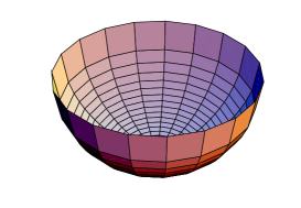
Figure 3: A curled-up brane in the background constant RR field strength with negative $f$.

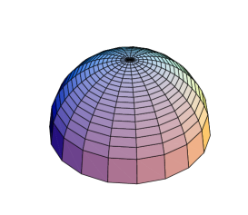
Figure 4: A curled-up brane with positive $f$.

Let us generalize the above result to the dielectric branes on which the nontrivial magnetic flux is turned on. Consider a D2-brane action with the magnetic field in the constant RR field strength (2.4),

$$S = -T_{{\rm D}2}\int dtdx^{1}dx^{2}\left[\sqrt{-\det(\eta_{\mu\nu}+\partial_{\mu}X\partial_{\nu}X+2\pi{\alpha^{\prime}}F_{\mu\nu})}-2fX\right]$$ (2.21)

$$= -T_{{\rm D}2}\int dtdx^{1}dx^{2}\left[\sqrt{1+(\partial_{\mu}X)^{2}+4\pi^{2}{\alpha^{\prime}}^{2}F_{12}^{2}}-2fX\right].$$

We have already ignored the time dependence. Assuming the radially symmetric configuration with $r\equiv\sqrt{(x^{1})^{2}+(x^{2})^{2}}$, the equations of motion becomes

$$2fr+\partial_{r}\left(\frac{r\partial_{r}X}{\sqrt{1+(\partial_{r}X)^{2}+4\pi^{2}{\alpha^{\prime}}^{2}F_{12}^{2}}}\right)=0,\quad\partial_{r}\left(\frac{2\pi{\alpha^{\prime}}F_{12}}{\sqrt{1+(\partial_{r}X)^{2}+4\pi^{2}{\alpha^{\prime}}^{2}F_{12}^{2}}}\right)=0.$$ (2.22)

It is easy to integrate these equations as in the same manner. the result is

$$\frac{\partial_{r}X}{\sqrt{1+(\partial_{r}X)^{2}+4\pi^{2}{\alpha^{\prime}}^{2}F_{12}^{2}}}=-fr+\frac{{c_{1}}}{r},\quad\frac{2\pi{\alpha^{\prime}}F_{12}}{\sqrt{1+(\partial_{r}X)^{2}+4\pi^{2}{\alpha^{\prime}}^{2}F_{12}^{2}}}={c_{2}}.$$ (2.23)

Here we have two integration constants ${c_{1}}$, ${c_{2}}$. Again, we simply put ${c_{1}}=0$ since the resultant configuration given below is consistent with the boundary condition (finiteness of the whole dielectric brane configuration). The second equation in (2.23) can be solved for $F_{12}$, giving a relation between $X$ and $F_{12}$ as

$$4\pi^{2}{\alpha^{\prime}}^{2}F_{12}^{2}=\frac{{c_{2}}^{2}}{1-{c_{2}}^{2}}\left(1+(\partial_{r}X)^{2}\right).$$ (2.24)

Substituting this into the first equation in (2.23), we obtain a (hemi-)spherical configuration $X=\sqrt{r_{0}^{2}-r^{2}}$ whose radius is given by

$$r_{0}=\frac{\sqrt{1-{c_{2}}^{2}}}{|f|}.$$ (2.25)

Certainly, the vanishing of the magnetic field ${c_{2}}=0$ leads back to the previous result.

The total magnetic flux on the D2-brane is equal to the number of D0-branes. This induced D0-brane charge is expressed as

$$\frac{N_{{\rm D0}}}{2}\mu_{{\rm D}0} = \mu_{{\rm D}2}\int 2\pi rdr(2\pi{\alpha^{\prime}}F)$$ (2.26)

$$= 2\pi\mu_{{\rm D}2}\int_{0}^{r_{0}}rdr\frac{{c_{2}}}{\sqrt{1-{c_{2}}^{2}}}\sqrt{1+(\partial_{r}X)^{2}}$$

$$= \mu_{{\rm D}2}\frac{2\pi}{f^{2}}{c_{2}}\sqrt{1-{c_{2}}^{2}}.$$

Here $\mu_{{\rm D}p}$ is the RR-charge of the D$p$-brane which is equal to the D$p$-brane tension $T_{{\rm D}p}=((2\pi)^{p}{\alpha^{\prime}}^{(p+1)/2}g)^{-1}$. We have only half of the total charge, $N_{{\rm D0}}/2$, since we made an integration over the hemisphere. Therefore we have

$$N_{{\rm D0}}=\frac{c_{2}\sqrt{1-{c_{2}}^{2}}}{\pi{\alpha^{\prime}}f^{2}}.$$ (2.27)

For a given background $f$ and a D0-brane charge $N_{\rm D0}$, it is easy to solve this relation for ${c_{2}}$. We have two solutions as

$${c_{2}}^{2}=\frac{1}{2}\pm\sqrt{\frac{1}{4}-\pi^{2}{\alpha^{\prime}}^{2}N_{{\rm D0}}^{2}f^{4}}.$$ (2.28)

Both are in the region $0<{c_{2}}<1$. Substituting this into the radius formula (2.25), we see that the larger ${c_{2}}$ is reproducing the radius of the dielectric brane $r_{\rm M}$(2.6), while the smaller one is giving the radius of the unstable solution $r_{\rm top}$ (2.7). Note that there is an upper bound for $|N_{{\rm D0}}|$, for a given background $f$. The existence condition for dielectric branes is

$$|N_{{\rm D0}}|\leq\frac{1}{2\pi{\alpha^{\prime}}f^{2}}.$$ (2.29)

2.3 Nucleation and expansion of spherical D$p$-brane

For the preparation for the calculation of the decay width of the dielectric branes in the next subsection, we develop the technique of constructing a bounce solution relevant to the tunnel effect. The simplest setting is the vacuum decay, that is, nucleation of a spherical D$p$-brane from nothing, in the background constant RR field strength. The computation of the decay width has been done already fifteen years ago by C. Teitelboim [11]. Here we reformulate his results in terms of our worldvolume coordinate choice for the later purpose. We find that our formulation also gives how the nucleated spherical brane decays for its expansion.

According to [14], the tunneling rate with the potential like Fig. 2 and Fig. 2 with a false vacuum is expressed as

$$\Gamma=c\exp[-S_{\rm E}],$$ (2.30)

where $S_{\rm E}$ is the Euclidean action for which the bounce solution of $S_{\rm E}$ is substituted. (The evaluation of the coefficient $c$ can be found in [15] and we shall not evaluate it in this paper.) The bounce solution should be a solution with the highest symmetry of the Euclidean action, thus it would be invariant under the $p+2$ dimensional spacetime rotation. This indicates that the bounce configuration of the Euclidean D$p$-brane (whose worldvolume is Euclidean and $p+1$ dimensional) is $S^{p+1}$. Let us study this in our language.

It is obvious that the curled-up branes formulated in the previous sections can be found in the same manner in the Euclidean space. The brane configuration of an Euclidean D$p$-brane in the constant RR $p+2$-form field strength (2.10) is governed by

$$S_{\rm E}=T_{{\rm D}p}\int d\tau d^{p}x\left[\sqrt{\det(\delta_{\mu\nu}+\partial_{\mu}T\partial_{\nu}T+2\pi{\alpha^{\prime}}F_{\mu\nu})}-2fT\right]$$ (2.31)

where $T$ is the fluctuation along the Euclidean time direction in the target spacetime, and we took the worldvolume coordinate along the spatial directions as before. $\tau$ is the worldvolume Euclidean time. We have assumed that the other scalar fields are vanishing.

For no worldvolume gauge fields turned on, the situation is completely same as what have been studied in Sec. 2.2. The only difference is the dimension. For the decay with the formation of the spherical D$p$-brane in the background $p+2$ form constant field strength, the relevant bounce solution is $S^{p+1}$ while the static configuration studied in Sec. 2.2 was $S^{p}$.

Following Sec. 2.2, the Euclidean action

$$S_{\rm E}=T_{{\rm D}p}\int d\tau d^{p}x\left[\sqrt{\det(\delta_{\mu\nu}+\partial_{\mu}T\partial_{\nu}T)}-2fT\right]$$ (2.32)

can be solved easily. For simplicity, we assume $f>0$ in the following. The solution is a $p+1$ dimensional hemisphere,

$$T=\sqrt{r_{0}^{2}-r^{2}},\quad r_{0}\equiv\frac{p+1}{2f}$$ (2.33)

where $r\equiv\sqrt{\tau^{2}+(x^{1})^{2}+(x^{2})^{2}+\cdots+(x^{p})^{2}}$. Then, the action evaluated is the same form as what has been found in [11]:

$$2S_{\rm E}=A(S^{p+1})r_{0}^{p+1}-2fV(S^{p+1})r_{0}^{p+2}.$$ (2.34)

Here the multiplication factor 2 is for the enveloping of two hemispheres. Using a relation $A(S^{p+1})=(p+2)V(S^{p+1})$, we can see that this $r_{0}$ (2.33) is what makes the action (2.34) be maximized.

The effect of our coordinate choice appears in the calculation of the brane decay after the nucleation. The expansion is due to the potential in Fig. 2, since the nucleation radius $(p+1)/2f$ (2.33) is larger than the radius at the top of the hill $p/2f$. Hence the configuration rolls down the hill toward the infinite radius.

The Minkowskian action is given as

$$S=T_{{\rm D}p}\int d^{p+1}\xi\left[-\sqrt{-\det(\eta_{MN}\partial_{a}\Phi^{M}\partial_{b}\Phi^{N})}+C(\Phi)\right].$$ (2.35)

We introduce a space-like parametrization of the worldvolume coordinates as before, by choosing a gauge

$$\xi^{1}=X^{1},\quad\cdots,\quad\xi^{p+1}=X^{p+1}.$$ (2.36)

This turns out to be useful for solving the equations of motion. We switch on only the fluctuation scalar for the target space time direction $T$. Then the action is reduced to

$$S=T_{{\rm D}p}\int A(S^{p})r^{p}dr\left[\sqrt{-1+(\partial_{r}T)^{2}}-2fT\right].$$ (2.37)

The equations of motion can be integrated in the same manner, giving

$$\frac{\partial_{r}T}{\sqrt{-1+(\partial_{r}T)^{2}}}=\frac{2f}{p+1}r+\frac{{c_{3}}}{r^{p}}.$$ (2.38)

As we will see shortly, the boundary condition at the nucleation time can be satisfied with the integration constant ${c_{3}}=0$. Then we have

$$\partial_{r}T=\frac{\displaystyle\frac{2f}{p+1}r}{\sqrt{-1+\displaystyle\frac{4f^{2}}{(p+1)^{2}}r^{2}}}.$$ (2.39)

Thus, appropriately choosing the zero of the time, we have the brane configuration

$$T=\sqrt{r^{2}-\frac{(p+1)^{2}}{4f^{2}}}.$$ (2.40)

In the above expression, the radius is $r=\sqrt{(X^{1})^{2}+\cdots+(X^{p+1})^{2}}$, as understood from the gauge choice (2.36). Therefore this equation shows that the shape of the solution is the hyperboloid in the target space. At $r=r_{0}=(p+1)/2f$, the initial velocity of the bubble is zero, as should be satisfied from the continuity condition with the nucleation radius (2.33). The bubble expands with the speed approaching that of light.

How the decay proceeds is shown in Fig. 5. The lower half of the figure is the nucleation part evolving in the Euclidean time, and the upper half is the expansion of the brane while the Minkowskian time. The picture is just like the birth of inflationary universes [16].

Figure 5: Nucleation of a spherical D-brane and its expansion. This figure is especially for the decay of a circular D-string ($p=1$) in the background RR 3-form field strength.

2.4 Decay width of dielectric D2-brane

Now we are ready to study the decay of a dielectric D2-brane. The relevant bounce configuration should satisfy the following conditions :

• The initial boundary condition is a static spherical D2-brane with magnetic flux and the radius (2.6).

• The highest symmetry is SO(3), thus the bounce configuration must be invariant under this.

• The final boundary condition is a spherical D2-brane whose radius is larger than the radius of the top of the hill, (2.7).

In the situation of the previous subsection, one needs no initial brane configuration and no magnetic flux, thus the symmetry was SO(4) and the brane configuration was a hemisphere. However, this time, $S^{2}$ of the dielectric D2-brane (the initial boundary condition) should be smoothly connected in the Euclidean spacetime. Hence the total shape of the solution must be a funnel.

Let us start with the Euclidean D2-brane action in the gauge chosen as before, (2.36). The action is

$$S_{\rm E}=T_{{\rm D}2}\int d^{3}\xi\left[\sqrt{\det(\delta_{\mu\nu}+\partial_{\mu}T\partial_{\nu}T+2\pi{\alpha^{\prime}}F_{\mu\nu})}-2fT\right],$$ (2.41)

where $\mu,\nu=1,2,3$, and $T$ is the scalar field representing the displacement along the Euclidean time direction. Turning on the gauge fields, we have

$$S_{\rm E}=T_{{\rm D}2}\int d^{3}\xi\left[\sqrt{1+(\partial_{i}T)^{2}+4\pi^{2}{\alpha^{\prime}}^{2}B_{i}^{2}+4\pi^{2}{\alpha^{\prime}}^{2}(B_{i}\partial_{i}T)^{2}}-2fT\right].$$ (2.42)

Since now the worldvolume is the Euclidean 3 dimensional space, the gauge field strength was arranged into a magnetic field. As mentioned before, the symmetry ansatz adopted here is SO(3), thus the Bianchi identity $\partial_{i}B_{i}=0$ is solved as

$$2\pi{\alpha^{\prime}}B_{i}=\partial_{i}\left(\frac{-{c_{5}}}{r}\right),$$ (2.43)

where $r\equiv\sqrt{(\xi^{1})^{2}+(\xi^{2})^{2}+(\xi^{3})^{2}}$. Using this magnetic field configuration, we need only to solve the equation of motion for $T$:

$$\partial_{i}\left(\frac{\partial_{i}T+4\pi^{2}{\alpha^{\prime}}^{2}B_{i}(B_{j}\partial_{j}T)}{\sqrt{1+(\partial_{i}T)^{2}+4\pi^{2}{\alpha^{\prime}}^{2}B_{i}^{2}+4\pi^{2}{\alpha^{\prime}}^{2}(B_{i}\partial_{i}T)^{2}}}\right)=-2f.$$ (2.45)

This can be integrated as

$$\frac{\partial_{r}T+4\pi{\alpha^{\prime}}^{2}B_{r}(B_{r}\partial_{r}T)}{\sqrt{1+(\partial_{r}T)^{2}+4\pi{\alpha^{\prime}}^{2}B_{r}^{2}+4\pi{\alpha^{\prime}}^{2}(B_{r}\partial_{r}T)^{2}}}=-\frac{2f}{3}r+\frac{{c_{4}}}{r^{2}},$$ (2.46)

where ${c_{4}}$ is the integration constant which we shall not put zero this time. Substituting the solution of $B_{i}$ (2.43), we obtain an expression for the solution $T$ as

$$\partial_{r}T=\frac{\displaystyle-\frac{2fr}{3}+\frac{{c_{4}}}{r^{2}}}{\sqrt{1-\displaystyle\frac{4f^{2}r^{2}}{9}+\frac{4f{c_{4}}}{3r}+\frac{1}{r^{4}}\left({c_{5}}^{2}-{c_{4}}^{2}\right)}}.$$ (2.47)

Before evaluating the action using this solution, let us investigate the meaning of the integration constants appearing in the solution. First, the magnetic field characterized by the monopole charge ${c_{5}}$ is expected to be related with the D0-brane charge induced on the dielectric brane. In our case, the dielectric brane is an initial state, and in the bounce solution above, this must be a fixed Euclidean time slice $T=T_{0}$. Because we adopt the rotational symmetry, this Euclidean time slice should corresponds to a certain fixed radius $r=r_{\rm M}$ in the worldvolume, through the solution (2.47). Therefore, the D0-brane charge can be evaluated from the magnetic field as

$$N_{{\rm D0}}\mu_{{\rm D}0} = \mu_{{\rm D}2}\int_{r=r_{\rm M}}2\pi{\alpha^{\prime}}F_{ij}\frac{1}{2}dx^{i}\wedge dx^{j}=4\pi{c_{5}}\mu_{{\rm D}2}.$$ (2.48)

Thus

$$N_{{\rm D0}}=\frac{1}{\pi{\alpha^{\prime}}}{c_{5}}.$$ (2.49)

Another integration constant ${c_{4}}$ can be determined from the initial boundary condition. Observe that for a given $f$ and a given $N_{\rm D0}$, $\partial_{r}T$ of the solution (2.47) diverges at two distinct radii $r_{1}$ and $r_{2}$ ($r_{1}<r_{2}$). This can be seen explicitly in numerical evaluation. Therefore, the solution (2.47) is actually a funnel-type which connects two $S^{2}$’s smoothly along the Euclidean time direction. One can see this more concretely by integrating the expression (2.47) by $r$. The result is shown in Fig. 7 and Fig. 7. The smaller radius $r_{1}$ must be the radius of the dielectric brane $r_{\rm M}$ which is given in (2.6). Hence the equation $\partial_{r}T=\infty$ (which is equivalent to the divergence of the denominator of (2.47)) should be satisfied with $r=r_{1}\equiv r_{\rm M}$, as

$$({c_{4}})^{2}+{c_{4}}\left(\frac{-4fr_{M}^{3}}{3}\right)+\frac{4f^{2}r_{M}^{6}}{9}-r_{M}^{4}-{c_{5}}^{2}=0.$$ (2.50)

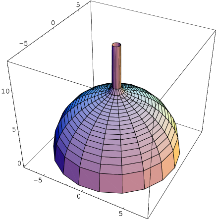
Figure 6: The bounce solution relevant for the decay of the dielectric brane with $N_{\rm D0}=1$ in the background $f=0.2$ in the unit $2\pi{\alpha^{\prime}}=1$. Note that this figure must be understood as upside-down.

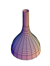
Figure 7: the bounce solution for different background $f=0.6$. The radius of the spout of the funnel is the same as that of Fig. 7, though the radius of the expanded large sphere is different due to the difference of the background RR field strength.

Interestingly, two solutions for ${c_{4}}$ of this equation are positive and negative, respectively. This can be seen from the fact that if we substitute ${c_{4}}=0$ on the left hand side of (2.50) it is always negative. For the negative ${c_{4}}$, $T(r)$ is monotonically decreasing as seen from (2.47), and we obtain a funnel-type brane configuration for the bounce, as shown in Fig. 7 and 7. (Note that our funnel is upside-down, since we have assumed $f>0$ for simplicity. In fact, this choice of the orientation of the funnel helps one to compute the Chern-Simons term of the Euclidean action.) On the other hand, if ${c_{4}}$ is positive, $\partial_{r}T$ is positive for small $r$ and becomes negative for large $r$. In this case there is a turning point for a certain $r$, and this results in an interesting brane configuration. In the next subsection, this solution is identified with the bounce solution for the nucleation of a dielectric brane from nothing.

In this subsection we use the negative solution for ${c_{4}}$. Note that, using this ${c_{4}}$ we can solve the equation $\partial_{r}T=\infty$ and get another solution of $r_{2}$ which is different from $r_{\rm M}$. This radius is that of the nucleated spherical D2-brane, and at that radius the expansion starts. In addition, this nucleated large spherical D2-brane has the same D0-brane charges as that of the original dielectric brane with $r=r_{M}$, since the computation (2.48) can be performed independent of its radius. Thus, we can say that throughout this nucleation and decay the charge of the D0-branes are conserved. The expansion is dictated by a hyperboloid worldvolume as in Fig. 5. The original D0-branes are brought away to the spatial infinity.

Fig. 7 indicates that the solution of this funnel type is actually a combination of the curled-up brane and a spike. For a large $r$, the brane configuration approaches to a hemisphere, while for a small $r$ the brane configuration can be approximated by a spike, or rather to say, a throat (volcano) solution of a D3-brane found in [12]. Here we have added newly the magnetic field, thus this throat part is a generalization of the solution constructed in [13] which is electrically charged.

The equation (2.47) can be integrated as

$$T=\int_{r_{D}}^{r}dr\frac{\displaystyle-\frac{2fr}{3}+\frac{{c_{4}}}{r^{2}}}{\sqrt{1-\displaystyle\frac{4f^{2}r^{2}}{9}+\frac{4f{c_{4}}}{3r}+\frac{1}{r^{4}}\left({c_{5}}^{2}-{c_{4}}^{2}\right)}},$$ (2.51)

where we have used the boundary condition $T(r_{2})=0$ to fix zero of time. The Euclidean action is then evaluated as

$$S_{\rm E}=T_{\rm D2}{\displaystyle\int_{r_{M}}^{r_{2}}4\pi r^{2}dr\left(\frac{1+\displaystyle\frac{{c_{5}}^{2}}{r^{4}}}{\sqrt{1-\displaystyle\frac{4f^{2}r^{2}}{9}+\frac{4f{c_{4}}}{3r}+\frac{1}{r^{4}}\left({c_{5}}^{2}-{c_{4}}^{2}\right)}}-2fT\right)}.$$ (2.52)

Note that in order to obtain the decay width we have to subtract the original action of the dielectric brane. Finally the decay width is given by

$$\Gamma\propto\exp\left(-\left[2S_{\rm E}-2T(r_{\rm M})E_{\rm dielectric}\right]\right)$$ (2.53)

where

$$E_{\rm dielectric}=4\pi T_{\rm D2}\sqrt{r_{M}^{4}+\pi^{2}{\alpha^{\prime}}^{2}N_{\rm D0}^{2}}.$$ (2.54)

Here the factor 2 in (2.53) is coming from the enveloping as before. $T(r_{\rm M})$ in front of $E_{\rm{dielectric}}$ is the “height” of the configuration in the Euclidean spacetime. Note that there is no potential term for $E_{\rm{dielectric}}$. This is because the potential energy from the background for the dielectric brane was already subtracted in the expression (2.52) since the integration region in (2.52) starts from $r_{\rm M}$, not from $0$.

To give an analytic expression for the decay width is difficult, thus here we shall give some numerical results. In the unit $2\pi{\alpha^{\prime}}=1$, the decay width depending on the background RR field strength is give as follows. For $N_{\rm D0}=1$, the magnitude of the exponent in the decay width formula (2.30) is given as

Figure 8: The energy potential (2.5) for various D0-brane charges ($N_{\rm D0}=0,1,\cdots,5$). The background field strength is fixed ($f=0.4$ in the unit $2\pi{\alpha^{\prime}}=1$).

$f$	0.99	0.9	0.8	0.6	0.4	0.2	0.1	0.01
$-{\rm exponent}/T_{\rm D2}$	0.129	3.074	9.650	45.89	213.1	1988	16466	1.6653$\times 10^{7}$

Note that $f=1$ in the unit $2\pi{\alpha^{\prime}}=1$ is the critical value for the existence of the dielectric brane with $N_{\rm D0}=1$, see (2.29). For comparison, we give the results for $N_{\rm D0}=0$ as

$f$	0.99	0.9	0.8	0.6	0.4	0.2	0.1	0.01
$-{\rm exponent}/T_{\rm D2}$	17.16	22.85	32.53	77.11	260.2	2081	16655	1.6655$\times 10^{7}$

The results lead us to the following observation : Existence of D0-branes makes the decay easier. This is very natural, since the potential barrier in the tunneling is lower for a larger number of D0-branes. The form of the potential for the dielectric branes with various D0-brane charges is shown in Fig. 8.

2.5 Nucleation of dielectric brane from nothing

In this subsection let us briefly discuss what is the positive ${c_{4}}$ solution of (2.50). As mentioned in the previous subsection, for the positive ${c_{4}}$, the derivative of the field $T$ has two regions: A certain value $r_{\rm c}$ exists with which in the region $r_{M}<r<r_{\rm c}$, $\partial_{r}T$ is positive, while in the region $r_{\rm c}<r<r^{\prime}_{2}$, $\partial_{r}T$ becomes negative. This $r^{\prime}_{2}$ is the solution of the equation $\partial_{r}T=\infty$ with given positive ${c_{4}}$.

The shape of the Euclidean brane configuration is given in Fig. 9. The shape is interesting by itself, a half slice of a doughnut surface. If we envelop it with the other half, then we obtain a complete doughnut surface. Note that the heights of the two $S^{p}$’s at $r=r_{M}$ and $r=r^{\prime}_{2}$ may not be the same. A numerical computation generically indicates the heights are in the relation $T(r_{M})-T(r^{\prime}_{2})>0$. This means, in Fig. 9 where we plot the half doughnut brane upside-down, the central peak is lower than the surrounding edge of a hemisphere. Thus to obtain a consistent doughnut after the enveloping, that is, to adjust two heights, one has to add a time-independent dielectric brane of the Euclidean time length $T(r^{\prime}_{2})-T(r_{M})$ on top of the central peak whose shape is a small $S^{2}$ at $r=r_{M}$. This additional configuration would be shown as a cylinder in Fig. 9. On the other hand, the brane configuration obtained here may be understood again as a combination of the curled-up brane and a spike (throat). The orientation of the curled-up brane is opposite to the one given in the previous subsection.

Figure 9: A bounce solution for a positive ${c_{4}}$ representing a nucleation of a dielectric brane and a large spherical brane. In this figure we plot $-T(r)$ in order to show inside the doughnut. We have chosen $f=0.5$ and $N_{\rm D0}=1$.

The interpretation of this configuration is much more interesting. This bounce solution represents nucleation of a pair of spherical branes, as seen from its Euclidean time slice. Two spherical branes necleated have the radii $r=r_{M}$ and $r=r^{\prime}_{2}$, and the former is a dielectric brane with the D0-brane charge $-N_{{\rm D}0}$ while the latter is a spherical brane which is about to decay, with an opposite D0-brane charge $N_{{\rm D}0}$. The reason why the former brane has the negative D0-brane charges is that the orientation of this brane surrounding the origin $r=0$ is opposite to the latter. Since the computation (2.48) does not depend on the radius to be used, the total D0-brane charge is conserved.

The outer spherical D2-brane would decay promptly with expansion, while the inner dielectric brane is meta stable and thus remain for a while. Since we have not considered the back reaction of the whole system, this dielectric brane is meta-stable, however if the whole system were in a 3 dimensional target space then the expansion of the outer brane may sweep out the background RR field and then the inner brane may collapse to form point-like $N_{\rm D0}$ D0-branes.

The computation of the decay width is straightforward, and we shall not give it here. Naively this decay rate must be slightly larger than the ordinary decay with no D0-brane charge given in Sec. 2.3. In Sec. 3.6, a similar situation will be found, where a pair of a brane and an antibrane decays with leaving a lower-dimensional branes.

3 Decay of brane-antibrane

3.1 Introductory remarks

The philosophy that all the brane physics in string theory can be deduced from brane-antibrane pairs via tachyon condensation has been supported successfully in K-theory and Sen’s conjecture [1]. On the basis of this, the investigation of the physics of the brane-antibrane system is now promoted to the dynamical level; that is, understanding of the dynamics of the tachyon decay. Since the annihilation of the brane-antibrane pairs is utilized for constructing cosmological inflation models of the braneworld [18], it is of importance to study how branes annihilate with antibranes in various situations in string/M theory.

Most of the study on the annihilation for the cosmological models has been made by use of the gravitational force between the branes. On the other hand, it has been reported that brane-antibrane pair can decay in another way: through the tunnel effect by creation of a throat between the brane and the antibrane [12, 13]. If the branes are free to move in the space, the time scale of the gravitational approach for the decay is much smaller than that of the decay via the tunnel effect, as noted in [12]. However, we place emphasis on the point that the final stage of the brane-antibrane decay must be the tachyon condensation since the pair annihilation and the vanishing of the tension are dictated by the tachyon condensation. Furthermore, there are certain situations where the latter time scale is dominant. Consider a brane configuration in which the asymptotic locations of the brane and the antibrane are fixed in such a way that the distance between the two cannot change (Fig. 11). Then these branes cannot approach each other by the gravitational force, hence the dominant time scale for the decay may be by the nucleation of the throat and the expansion of the throat to make the brane-antibrane vanish (see Fig. 11).

The decay of unstable systems through the tunnel effect may be characterized by the height of the potential barrier. In the decay of the brane-antibrane, the top of the potential must be a non-trivial brane configuration. (For the decay of the dielectric brane, this is the spherical brane configuration of the point A’ in Fig. 2.) This was explicitly constructed in [12, 13], and called sphaleron solutions. These sphalerons were solutions in the Born-Infeld-Higgs system on a single D-brane. The scalar field configuration of their solution shows a shape of a volcano, a “half” of the throat attached to the body of the flat D-brane.

However, as mentioned, the main contribution to the brane-antibrane decay must be the condensation of the tachyon which comes from an excitation of a string connecting the brane and the antibrane. In this section, we reconsider this formation of the throat from the viewpoint of the tachyon condensation. The formation of the throat is the result of the quantum tunnel effect. We investigate this tunnel effect and compute its probability, by using the effective field theory of the tachyon fields living on the brane-antibrane. We show the existence of a bounce solution in the tachyon field theory, and the brane configuration formed by this bounce solution as its final state is found to be a throat-like. Inside the throat, the tachyon sits at the true vacuum known as the closed string vacuum, thus there is no brane there. The throat itself is a spherical bubble made of a domain wall. Outside the bubble the tachyon expectation value is zero, thus the brane and the antibrane has not vanished yet there. After the nucleation of the throat, the tachyon configuration “rolls down” the potential hill.

Figure 10: An example configuration in which the asymptotic distance between the brane and the antibrane is fixed. Four vertical lines are D5-branes on which the D3-brane and the anti-D3-brane have ends.

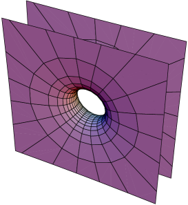
Figure 11: The “throat” which connects the brane and the antibrane is formed. The decay proceeds with the expansion of the radius of this throat.

The analysis in this section proceeds in the following way. First, we derive the action of the relevant tachyon system of the separated brane-antibrane. We find that the parallel brane-antibrane corresponds to a false vacuum (a local minimum of the tachyon potential) of the tachyon field theory. We apply Coleman’s method for describing the decay of the false vacuum via the tunnel effect, and construct a relevant bounce solution for the Euclidean tachyon field theory. We show that the Euclidean action evaluated with this bounce solution is reproducing a naive energy of a throat of the Euclidean brane computed by its tension times the area (volume). The radius $R_{0}$ of the throat of the bounce solution is at the order of the brane separation, $R_{0}\sim l$. Interestingly, the energy of the throat is very similar to what was found in Sec. 2.3. Instead of the background RR field strength $f$ in Sec. 2.3, here we have the brane separation parameter $l$. The correspondence is almost $l\sim f^{-1}$. We may use this similarity to argue how the decay proceeds after the nucleation of the throat.

3.2 Naive prospect

Before going to the detailed study of the decay width using the tachyon condensation, here we shall give a naive estimation of the decay width. This naive prospect is based only on the tensions and shapes of the branes. Later we will see that this prospect coincides with the estimation by the tachyon condensation.

First, the tunnel effect is caused by the bounce solution which has the highest symmetry in the Euclideanized theory and satisfies appropriate boundary conditions. In our case, starting from the parallel D$p$-brane and anti-D$p$-brane, we expect that the resultant brane configuration after the tunneling will be a throat connecting two flat branes. This is shown in Fig. 12. Therefore, the bounce solution should have the Euclidean (p+1)-dimensional worldvolume, and thus this bounce configuration is effectively a static configuration of a D$(p+1)$-brane. As shown in Fig. 12, the nucleated throat is found in the $\tau=0$ (Euclidean) time slice. According to Coleman’s method which will be explained and generalized in detail in the next subsection, the decay width by this bounce solution is given by (2.30). In our case, as we stated before, the Euclidean action which is to be substituted is just the Euclidean worldvolume area times the brane tension. Thus, for the brane configuration given in Fig. 12, the action is given as

$$S_{\rm E}=\left[A(S^{p})lR_{0}^{p}-2V(S^{p})R_{0}^{p+1}\right]T_{{\rm D}p}=\left[A(S^{p})R_{0}^{p}-2l^{-1}V(S^{p})R_{0}^{p+1}\right]T_{{\rm D}p}l.$$ (3.1)

Note that the first term is the action of the throat whose section is $S^{p}$, and the second term is for two holes in the parallel brane-antibrane. The bounce solution must be the extremum of the action, thus we can determine the radius $R_{0}$ by $\delta S_{\rm E}/\delta R_{0}=0$, which gives

$$R_{0}=\frac{p}{2}l.$$ (3.2)

Interestingly, the expression (3.1) is very similar to what we encountered in the evaluation of the action for the nucleation of the spherical branes in the constant RR field strength (2.34). This analogy will be checked further by confirming the expression (3.1) in the tachyon condensation in the following subsections. The intuition of the analogy will help us to find the decay width of the brane-antibrane while leaving a lower dimensional branes in Sec. 3.6 and to understand how the decay proceeds after the nucleation of the throat.

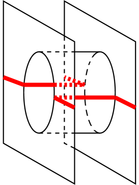
Figure 12: A naive expectation of the bounce solution. Here we draw a figure for $p=1$. The throat is a cylinder, and it makes a hole in each Euclidean D1-brane worldvolume. The thick lines denote a Euclidean time slice $\tau=0$, which represents a nucleated throat between the two D1-branes.

3.3 Description of brane-antibrane by tachyon field

Let us state our situation more precisely : a D$p$-brane and an anti-D$p$-brane are sitting with a distance $l$, in parallel. If the distance $l$ is large enough, then the tachyon mode between the two should go away, since the complex tachyon is coming from the string suspended between the two branes and thus that string acquire a mass lift when two branes are distant. In fact, the mass of the lowest excitation mode of the string connecting these branes is given by

$$m^{2}=\left(\frac{l}{2\pi{\alpha^{\prime}}}\right)^{2}-\frac{1}{2{\alpha^{\prime}}}.$$ (3.3)

Therefore evidently this tachyonic mode becomes massive when the separation $l$ becomes larger than $\sqrt{2\pi^{2}{\alpha^{\prime}}}$.

However, intrinsically the system we are considering must be unstable, since if these two branes annihilate then the total energy of the system will decrease. Therefore, the stability of the separated brane-antibrane system considered above must be perturbative, and we expect that the true vacuum of the system will be obtained nonperturbatively. Although perturbative tachyon potential has been obtained from the string scattering amplitude in this background brane-antibrane [21], we need nonperturbative information on the tachyon potential. Fortunately, exact tachyon potentials have been computed in the boundary string field theory (BSFT) [22], and a part of Sen’s conjectures have been verified [23]. The tachyon effective field theories obtained as a derivative truncation of BSFT actions are found to reproduce a partial spectra of D-branes from tachyon defects [24]. We shall use this tachyon effective action for our investigation in the following.

In order to obtain the brane-antibrane configuration to be dealt with, first consider the D$(p\!+\!1)$-brane - anti-D$(p\!+\!1)$-brane on top of each other. The action is given by [25] as

$$S=T_{{\rm D}(p+1)}\int\!d^{p+2}x\;e^{-|T|^{2}}\left[1+2{\alpha^{\prime}}|D_{\mu}T|^{2}+\frac{(\pi{\alpha^{\prime}})^{2}}{4}(F_{\mu\nu}^{(-)})^{2}\right],$$ (3.4)

where we employed the two-derivative truncation of the BSFT. The complex tachyon field $T$ is charged under the gauge group $U(1)$ associated with the gauge field

$$A^{(-)}_{\mu}\equiv A^{{\rm D}(p+1)}_{\mu}-A^{{\rm antiD}(p+1)}_{\mu},$$ (3.5)

and we ignored another combination of the gauge fields since it is irrelevant for our following discussion. Now, turn on the constant Wilson line $A_{p+1}=A$ for this gauge field and take a T-duality along $x_{p+1}$ axis. Then, the gauge field is mapped to the Higgs field which measures the distance between the two, and the distance is given by the absolute value of the Wilson line. If we neglect all the fields other than the tachyon field, then we obtain an action

$$S=2T_{{\rm D}p}\int\!d^{p+1}x\;e^{-|T|^{2}}\left[1+2{\alpha^{\prime}}|\partial_{\mu}T|^{2}+2{\alpha^{\prime}}A^{2}|T|^{2}\right].$$ (3.6)

It is very easy to see that this action has the desired properties discussed above. The potential term of this action has an expansion

$$V(T)=e^{-|T|^{2}}\left[1+2{\alpha^{\prime}}A^{2}|T|^{2}\right]=1+\left(2{\alpha^{\prime}}A^{2}-1\right)|T|^{2}+{\cal O}(T^{4}),$$ (3.7)

Thus the mass for this tachyon field is given by

$$m^{2}=A^{2}-\frac{1}{2{\alpha^{\prime}}}.$$ (3.8)

One can see the precise correspondence between (3.3) and this equation, and we have

$$A=\frac{l}{2\pi{\alpha^{\prime}}}.$$ (3.9)

Furthermore, the above potential tells us that, if $A$ is large enough then the system is perturbatively stable at $T=0$, but the true vacuum of the system is lying at $T=\infty$ which is so-called closed string vacuum, i.e. where two D$(p\!+\!1)$-branes do not exist. The profile of the potential $V(T)$ is shown in Fig. 13.

Figure 13: Potential (3.7) with $A=2$ and $2{\alpha^{\prime}}=1$.

From this respect, the annihilation of two distant branes is just the transition from the false vacuum $T=0$ to the true vacuum $T=\infty$, through the potential barrier. Let us consider the properties of this potential barrier. The height of the potential is at $T_{\rm top}=\sqrt{1-1/(2{\alpha^{\prime}}A^{2})}$, and if we assume that $l\gg l_{s}\equiv\sqrt{{\alpha^{\prime}}}$ where $l_{s}$ is a string length, this is approximated by $T_{\rm top}\sim 1$. The potential hight at this point is $V_{\rm top}\sim 2{\alpha^{\prime}}A^{2}/e$. Thus if the distance between the two branes become large, the potential barrier grows (as $\sim l^{2}$). This is very natural. For a possible BSFT correction to this tachyon potential, see Appendix A.

3.4 Decay width of brane-antibrane

3.4.1 Coleman’s computation in arbitrary dimension

The prescription on how to compute the decay width of the false vacuum was given by S. Coleman [14]. Here we summarize his results [14, 26] and generalize it to the case of field theories with arbitrary spacetime dimensions. The system considered in [14] is a scalar field theory with an action

$$S=\int d^{p+1}x\left[-\frac{1}{2}\left(\partial_{\mu}\Phi\right)^{2}+U(\Phi)\right].$$ (3.10)

Here we have generalized it to the system of $p+1$ dimensional spacetime, and $U(\Phi)$ is assumed to have a false vacuum. One may imagine the potential of Fig. 13 as $U(\Phi)$. Suppose that one starts with a homogeneous false vacuum. Then the tunneling toward the true vacuum is described by a bounce configuration which is a solution of an Euclidean equation of motion. The principle to have that bounce solution is the highest symmetry, as mentioned in the previous section, that preserves all of the boundary conditions. In our case, the highest symmetry is the rotational invariance $SO(p+1)$ in the Euclidean space. Thus the bounce solution is a true vacuum bubble. The surface of the bubble consists is a domain wall, and the inside of the bubble is true vacuum while the outside sits still at the false vacuum. The decay width is given in the formula (2.30). For a high potential barrier, we may adopt the thin wall approximation, then the result is

$$S_{\rm E} = \int_{0}^{\infty}A(S^{p})\rho^{p}\left[\frac{1}{2}\left(\frac{d\Phi}{d\rho}\right)^{2}+U(\Phi)\right]d\rho$$ (3.11)

$$= A(S^{p})R^{p}S_{1}-V(S^{p})R^{p+1}\epsilon$$

where $R$ is the radius of the bubble estimated later. In this approximation, the “wall energy” $S_{1}$ is approximated by that of the one dimensional system,

$$S_{1}\equiv\int_{\Phi_{0}}^{\Phi_{1}}d\Phi\sqrt{2U(\Phi)}.$$ (3.12)

Here $\Phi_{0}$ is the value of the field giving the false vacuum of the potential $U(\Phi)$, while $\Phi_{1}$ is that for the true vacuum. The parameter $\epsilon$ is the difference of the energies of the two local minima,

$$\epsilon\equiv U(\Phi_{0})-U(\Phi_{1}).$$ (3.13)

The thin wall approximation is applicable if [14]

$$\frac{S_{1}\mu}{\epsilon}\gg 1,$$ (3.14)

where $\mu$ is the mass scale of the system. This $\mu$ is given by the coefficients of the mass term evaluated at the top of the potential.

Since the energy of the bubble is written by its radius, we can determine the radius of the bubble as a solution of the equation

$$\frac{\delta S_{\rm E}}{\delta R}=0.$$ (3.15)

For arbitrary dimensions, we obtain

$$R=\frac{p}{p+1}\frac{A(S^{p})}{V(S^{p})}\frac{S_{1}}{\epsilon}.$$ (3.16)

Then, using this radius, the Euclidean action is finally evaluated as

$$S_{\rm E}=\frac{p^{p}}{(p+1)^{p+1}}\frac{(A(S^{p}))^{p+1}}{(V(S^{p})^{p})}\frac{(S_{1})^{p+1}}{\epsilon^{p}}=\frac{p^{p}}{p+1}\frac{2\pi^{(p+1)/2}}{\Gamma\left(\frac{p+1}{2}\right)}\frac{(S_{1})^{p+1}}{\epsilon^{p}}.$$ (3.17)

In the next subsection, we apply this result for the decay of the brane-antibrane.

3.4.2 Application to ours

To apply the generalized Coleman’s computation to our situation, there exists two obstacles coming from the difference between our action (3.6) and a usual action (3.10). First, our system has a complex tachyon field while (3.10) is a real scalar field. Second, the tachyon action (3.6) has an unusual kinetic term.

For the first difference, here we simply assume that the relevant tachyon bounce solution is real. The vanishing of the imaginary part of the tachyon is consistent with the tachyon equations of motion, and furthermore this is a very natural ansatz since we are considering no lower dimensional D-brane left after the tachyon condensation. (The lower dimensional D-branes which are stable may appear after the tachyon condensation as topological defects [1], and this needs complex tachyon configurations.) For the real tachyon field,

$$S=2T_{{\rm D}p}\int d^{p+1}xe^{-T^{2}}\left[1+2{\alpha^{\prime}}(\partial_{\mu}T)^{2}+2{\alpha^{\prime}}A^{2}T^{2}\right].$$ (3.18)

Then, with the real tachyon, we can redefine the tachyon field so that the action have a canonically normalized kinetic term:

$$\Phi\equiv\sqrt{8{\alpha^{\prime}}T_{{\rm D}p}}\int_{0}^{T}ds\;e^{-s^{2}/2}.$$ (3.19)

Note that, although the original true vacuum of the tachyon is at the infinity $|T|=\infty$, this redefinition makes it to be placed at a finite value of the new field $\Phi$. In fact, two local minima are

$$\Phi_{0}=0,\quad\Phi_{1}=\sqrt{4\pi{\alpha^{\prime}}T_{{\rm D}p}}.$$ (3.20)

However, the field redefinition does not change the energy difference

$$\epsilon=2T_{{\rm D}p}.$$ (3.21)

The form of the potential written by this new field is shown in Fig. 14.

Figure 14: The potential $U(\Phi)/2T_{{\rm D}p}$ with $A=2$, $2{\alpha^{\prime}}=1,8{\alpha^{\prime}}T_{{\rm D}p}=1$ for simplicity. The true vacuum (depicted as a blob) is located at the finite distance $\Phi_{1}$.

We need to determine the scale parameter $\mu$ of the theory by studying the behaviour of the potential around its maximum. The potential written in terms of the tachyon is

$$U=2T_{{\rm D}p}e^{-T^{2}}(1+2{\alpha^{\prime}}A^{2}T^{2}).$$ (3.23)

For the high potential, we have large ${\alpha^{\prime}}A^{2}$, hence the top of the hill is at $T\sim 1$. There

$$\frac{\delta^{2}U}{\delta T^{2}}\sim-2T_{{\rm D}p}\frac{8{\alpha^{\prime}}A^{2}}{e}.$$ (3.24)

The redefinition (3.19) at $T=1$ gives

$$\delta\Phi=\sqrt{8{\alpha^{\prime}}T_{{\rm D}p}}\;e^{-1/2}\delta T,$$ (3.25)

thus

$$U-U_{\rm top}\sim-A^{2}(\delta\Phi)^{2}$$ (3.26)

hence the mass scale evaluated at the top of the hill is given by

$$\mu\sim 2A.$$ (3.27)

Next, we evaluate $S_{1}$. Writing $S_{1}$ by integration with $T$,

$$S_{1} = \int_{0}^{\sqrt{4\pi{\alpha^{\prime}}T_{{\rm D}p}}}d\Phi\sqrt{2U(\Phi)}$$ (3.28)

$$= \int_{0}^{\infty}dTe^{-T^{2}/2}\sqrt{8{\alpha^{\prime}}T_{{\rm D}p}}\sqrt{2\cdot 2T_{{\rm D}p}e^{-T^{2}}(1+2{\alpha^{\prime}}A^{2}T^{2})}$$

$$= 4\sqrt{2{\alpha^{\prime}}}T_{{\rm D}p}\int_{0}^{\infty}dTe^{-T^{2}}\sqrt{1+2{\alpha^{\prime}}A^{2}T^{2}}.$$

In this expression, it is easy to see the validity of the thin wall approximation (3.14), since the left hand side of (3.14)

$$\frac{S_{1}\mu}{\epsilon}=4\sqrt{2{\alpha^{\prime}}A^{2}}\int_{0}^{\infty}dTe^{-T^{2}}\sqrt{1+2{\alpha^{\prime}}A^{2}T^{2}}$$ (3.29)

is much larger than $1$ if $2{\alpha^{\prime}}A^{2}$ is large. Let us continue the evaluation of $S_{1}$. We use the steepest-descent method by defining the integrand as an exponential form,

$$e^{-T^{2}}\sqrt{1+2{\alpha^{\prime}}A^{2}T^{2}}\equiv e^{f(T)}.$$ (3.30)

This $f(T)$ has a maximum at $T\sim\sqrt{1/2}$ where the second order derivative is $\delta^{2}f/\delta T^{2}\sim-4$. Thus the integration of (3.28) is evaluated as

$$\int_{0}^{\infty}dTe^{-T^{2}}\sqrt{1+2{\alpha^{\prime}}A^{2}T^{2}} \sim \int_{0}^{\infty}dTe^{-1/2}\sqrt{1+{\alpha^{\prime}}A^{2}}e^{-2(\delta T)^{2}}$$ (3.31)

$$\sim \sqrt{\frac{1+{\alpha^{\prime}}A^{2}}{e}}\int_{-\sqrt{1/2}}^{\infty}d(\delta T)e^{-2(\delta T)^{2}}$$

$$\sim c_{0}\sqrt{\frac{{\alpha^{\prime}}A^{2}}{e}},$$

where numerically $c_{0}\sim 1.15$. Therefore, we obtain

$$S_{1}\;\sim\;4\sqrt{2{\alpha^{\prime}}}T_{{\rm D}p}c_{0}\sqrt{\frac{{\alpha^{\prime}}A^{2}}{e}}\;\sim\;0.628\;T_{{\rm D}p}l.$$ (3.32)

Then we obtain the radius (3.16) of the nucleated bubble as

$$R\;\sim\;\frac{2\sqrt{2}c_{0}}{2\pi\sqrt{e}}p\;l\;\sim\;0.314p\;l.$$ (3.33)

We see that this radius is given by $\sim l$, The naive estimation (3.2) gives a correct dependence on the brane separation $l$, although we have another dimensionful parameter $l_{s}$. Finally, the decay width is given by the Euclidean action,

$$S_{\rm E} = \frac{p^{p}}{p+1}\frac{1}{\Gamma\!\left(\frac{p+1}{2}\right)}\frac{1}{2^{p-1}\pi^{(p+1)/2}}\left(\frac{2\sqrt{2}\cdot c_{0}}{\sqrt{e}}\right)^{p+1}l^{p+1}T_{{\rm D}p}$$ (3.34)

$$= \frac{p^{p}}{p+1}\frac{1}{\Gamma\!\left(\frac{p+1}{2}\right)}\frac{1}{2^{2p-1}\pi^{3(p+1)/2}}\left(\frac{2\sqrt{2}\cdot c_{0}}{\sqrt{e}}\right)^{p+1}\left(\frac{l}{l_{s}}\right)^{p+1}\frac{1}{g}.$$

From the result above, especially the coincidence with the naive prospect in Sec. 3.2, we claim that this bubble of the true vacuum corresponds to a throat connecting the brane and the antibrane. To make sure that this claim is correct, in the next subsection we study the scalar field configuration with this tachyon bubble, since the shape of the throat is determined by this scalar field on the brane-antibrane.

As we noted, the expression for the Euclidean action (3.1) evaluated by the bounce solution is very similar to what we have found in the nucleation of a spherical D$p$-brane in the constant RR field strength. Thus from this observation it is easy to guess the fate of the nucleated throat in the brane-antibrane, from Fig. 5. The tachyon at each radius outside of the throat rolls down the hill in due order, and the throat (which is the tachyon domain wall) expands. The speed of the expansion of the throat radius may approach the speed of light, then the brane-antibrane is swept out to vanish.

3.5 Inclusion of scalar field

Originally the tachyon field is interacting with infinitely many other fields which are also excitations of the strings. Among them, massless fields such as scalar fields and vector gauge fields are of importance, and we had to incorporate these fields to make the description precise. However, it is of course difficult to treat all the modes at the same time, thus we have considered only the tachyon mode. We have seen that this approximation works well, that is, we have found that the decay width of the brane-antibrane is that of the naive computation by making a throat.

Now let us try to incorporate the scalar field in this system. We shall not consider the gauge fields because it is relevant for the situation where some lower dimensional D-branes are left after the tachyon condensation. Here we consider only the complete annihilation of the brane-antibrane pair. For the case leaving smaller D-branes, see Sec. 3.6.

The scalar field is actually what was originally studied in [12, 13], and in these papers the existence of a kind of sphaleron (a throat solution) was shown. Therefore we expect that incorporation of the scalar field $X$ into our system does not change the physical results. The relevant scalar field here is the combination $X^{\rm(D4)}-X^{\rm(antiD4)}\equiv X$ which measures the distance between the two branes. This can be easily seen from the T-duality which we considered in Sec. 3.3. The value of the field $X$ should be finite.

The Euclidean action of the scalar field interacting with the tachyon is written as

$$S=2T_{{\rm D}p}\int\!d^{p+1}x\;e^{-|T|^{2}}\left[\frac{(\pi{\alpha^{\prime}})^{2}}{2}(\partial_{\mu}X)^{2}+X^{2}|T|^{2}\right].$$ (3.35)

We employed again an action which is two-derivative truncation of the BSFT results [25]. Since it is difficult to solve the full equations of motion, we regard the tachyon solution as an background and consider how the scalar field behaves on this background.

Therefore, first let us see how the solution of the tachyon equations of motion behaves in various regions. As in the previous sections, we assume that the tachyon field is a real function of $r$ where $r$ is a radial coordinate of the Euclidean D$p$-brane worldvolume. We consider the case $p=2$ for simplicity. Under this assumption, we obtain the equation of motion as

$$T\left(\frac{1}{2{\alpha^{\prime}}}-A^{2}-(\partial_{r}T)^{2}+A^{2}T^{2}\right)+\partial_{r}^{2}T+\frac{2}{r}\partial_{r}T=0.$$ (3.36)

The last two terms come from the Laplacian acting on $T$.

Let us study the asymptotic behaviour of the solution. The physical requirement is that, in the region with large $r$, $T$ must sit at the false vacuum $T=0$. Neglecting the terms of the higher order in $T$ and also the last term for the large $r$, we obtain an appropriate asymptotic solution

$$T\propto\exp\left[-r\sqrt{A^{2}-\frac{1}{2{\alpha^{\prime}}}}\right].$$ (3.37)

Using this behaviour as an input at large $r$, we can solve the equations of motion numerically. The result is very interesting, as shown in Fig. 15. One observes that at a certain $R$ the solution $T$ diverges to the infinity.

Divergence of $T$ is equivalent to the approach to the true vacuum $\Phi=\Phi_{1}$. Therefore, the numerical solution in Fig. 15 is actually a domain wall solution which interpolates from the false vacuum to the true vacuum. In the region $r<R$, the tachyon sits at the true vacuum, and thus the open string physics there is expected to disappear completely. This means that there is no D2-brane there. We expect that after the tunneling the D2-branes are connected by making a throat between them. Inside the throat radius, we have only the holes.

Figure 15: A numerical solution to the equation of motion with $A=5$ in the unit $2{\alpha^{\prime}}=1$. The boundary condition is chosen as $T(r\!=\!5)=0.01,T^{\prime}(r\!=\!5)=-\sqrt{A^{2}-1}\;T(r\!=\!5)$, according to the asymptotic solution (3.37).

Then, let us consider the scalar field behaviour in this tachyon background of the bounce solution. The equations of motion for the scalar field $X$ becomes

$$2e^{-|T|^{2}}|T|^{2}X-(\pi{\alpha^{\prime}})^{2}\partial_{\mu}\left(e^{-T^{2}}\partial_{\mu}X\right)=0.$$ (3.38)

We substitute the bounce solution for $T$. Around $r=r_{0}$ the tachyon $T$ diverges, and generically near the divergent point $|\partial_{r}T|$ is much larger than $T$ itself. Thus we expect that the dominant behaviour of $\Phi$ around $r=r_{0}$ comes from the second term of the equation above. Neglecting the first term, we have

$$\partial_{r}\left(e^{-T^{2}}r^{2}\partial_{r}X\right)=0.$$ (3.39)

Here we have used the assumption that the scalar field is rotationally symmetric. Then it is easy to find a solution for the scalar field as

$$\partial_{r}X=e^{T^{2}}\frac{c}{r^{2}}.$$ (3.40)

This indicates that the derivative of the scalar field diverges at $r=R$. This result is very consistent, since from the tachyon bounce solution we expected that at $r=R$ the two branes are connected and making a throat. At that point the gradient of the scalar field must be divergent. Thus we have a consistency.

On the other hand, we can solve the equations of motion (3.38) asymptotically by substituting the asymptotic tachyon solution (3.37). The resultant asymptotic behaviour of $X$ is $\sim 1/r$ which is the same as what was found in the “sphaleron” solution in [12]. So we have another consistency. The difference between ours and [12] is that the nontrivial throat part in [12] comes from the nonlinearity of the action in $X$, while the divergence of $\partial_{r}X$ in our case is due to the coupling with the tachyon.

Unfortunately, we don’t have any indication that the distance between the two branes which must be given by integrating $\partial_{r}X$ is actually the parameter $l$. Perhaps in order to see this we have to study the full equations of motion of the interacting system including ${\alpha^{\prime}}$ corrections.

3.6 Annihilation leaving topological defect

Up to here in this section we have assumed a real configuration of the tachyon field. If we consider a nontrivial winding of the complex tachyon field onto the infinity of the 2-dimensional subspace of the worldvolume, then we may describe a situation where the tachyon condensation leaves a D$(p\!-\!2)$-brane.

Let us consider especially the case with $p=2$ for simplicity. In this case, a D0-brane may be left after the condensation. It is easy to write a tachyon action under the assumption that

$$T=t(r)e^{i\theta}$$ (3.41)

where $t(r)$ is a real function of $r\equiv\sqrt{(x^{1})^{2}+(x^{2})^{2}}$, and $\tan\theta\equiv x^{2}/x^{1}$, which are the polar coordinates. This nontrivial winding corresponds to a single D0-brane charge sits at the origin. The Euclidean action written with this ansatz is similar to what we have considered for the real tachyon, though the boundary condition is slightly different: to guarantee the single-valuedness for the tachyon at the origin $r=0$, we must have $t(0)=0$. Because of this constraint, there remains a small part of the false vacuum even inside the throat. This small part is actually expected to be a D0-brane. Here we shall not perform the explicit evaluation of the Euclidean action in this case. Instead, we use the analogy with the brane configuration found in Sec. 2.5 to evaluate the Euclidean action naively.

Since the defect remaining inside the throat is expected to be a D0-brane, thus the total action in the thin wall approximation would be

$$S_{\rm E}=-V(S^{2})R^{3}\epsilon+A(S^{2})R^{2}S_{1}+2RT_{{\rm D}0},$$ (3.42)

here the last term is coming from the D0-brane. Then solving the stationary condition for $R$, we obtain

$$R=\frac{S_{1}}{\epsilon}+\sqrt{\frac{S_{1}}{\epsilon}+\frac{T_{{\rm D}0}}{2\pi\epsilon}}.$$ (3.43)

Using the previous result

$$\frac{S_{1}}{\epsilon}=\frac{2\sqrt{2}c_{0}}{\sqrt{e}}{\alpha^{\prime}}A=\frac{\sqrt{2}c_{0}}{\sqrt{e}\pi}l,$$ (3.44)

we obtain the Euclidean action as

$$S_{\rm E}=\frac{16\pi}{3}\frac{(S_{1})^{3}}{\epsilon^{2}}+\Delta S$$ (3.45)

where

$$\Delta S=\frac{16\sqrt{2}c_{0}}{\sqrt{e}}l_{s}^{2}\;l\;T_{{\rm D}2}.$$ (3.46)

The ratio of the decay width is given by $\exp(-\Delta S)$, and we observe that it gets difficult to decay when the D0-brane is left, and its ratio is almost the exponential of minus of $l/l_{s}g$. Our computation here is using a plausible but conjectural approximation, and precise computation may need the gauge field on the D2-branes. However we believe that our computation is qualitatively correct.

3.7 Decay of D0-$\overline{\mbox{D0}}$

Our computation of the decay width of the D$p$-brane and the anti D$p$-brane is valid only for $p\geq 1$, since we have utilized nontrivial bounce solutions in field theories. For the case $p=0$, that is, a pair of a D0-brane and an anti-D0-brane, then we have no spatial worldvolume, thus we have to use the quantum mechanics to describe the annihilation of these D0-branes.

The bounce solution is just a virtual particle whose position is described by $\Phi$ and which rolls down the hill of $-U(\Phi)$ in one dimensional space. From the form of the potential we have a bouncing point $\Phi_{b}$, and the Euclidean action is evaluated as

$$S_{\rm E}=2\int_{0}^{\Phi_{b}}d\Phi\sqrt{2\left(U(\Phi)-U(0)\right)},$$ (3.47)

where $\Phi_{b}$ satisfies $U(\Phi_{b})=U(0)$. To give the explicit computation we rewrite this expression in terms of $T$ as

$$S_{\rm E}=8\sqrt{2}T_{{\rm D}0}\int_{0}^{T_{b}}dTe^{-T^{2}/2}\sqrt{e^{-T^{2}}(1+2{\alpha^{\prime}}A^{2}T^{2})-1}$$ (3.48)

where $T_{b}$ is the corresponding bounce point. We shall give here only the numerical result. For a given string coupling constant $g=0.1$ and in the unit $l_{s}=1$, The bouncing point and the decay width are shown in the following table.

$l$	20	10	5	$\sqrt{2}\pi$	2
$T_{b}$	2.129	1.638	0.6748	0	—
$S_{\rm E}$	2.1022	0.8450	0.06761	0	—

Note that below the critical separation $l=\sqrt{2}\pi l_{s}$, there appears a tachyonic mode at the false vacuum, thus the tunneling computation becomes invalid in the region $l<\sqrt{2}\pi l_{s}$.

We point out here that there exists another interesting decay mode which is a pair creation of another D0-brane anti-D0-brane pair. This pair may be created since the original D0-brane anti-D0-brane pair produces a background RR gauge field configuration between them as

$$C_{0}(x)=60\pi^{3}g\left(\left(\frac{l_{s}}{\frac{l}{2}-x}\right)^{7}-\left(\frac{l_{s}}{\frac{l}{2}+x}\right)^{7}\right).$$ (3.49)

Here we describe the RR gauge potential only along the straight line connecting these two background D0-branes, since only this information is necessary for the later purpose. The coordinate $x$ specifies the point on the line, and we have chosen its zero at the middle point of these background D0-branes. As we have seen in Sec. 2, in the constant RR ($p+2$)-form field strength the nucleation of a spherical D$p$-brane may occur. Now we are not in the constant field strength but in a varying background RR field strength, thus a pair creation via non-trivial (non-spherical) bounce configuration is expected. In fact, the curvature of the spherical D-branes is determined only by the background value of the RR field strength, therefore in this case of the D0-branes a non-trivial worldline in the Euclidean space may be determined by the RR configuration (3.49).

Since the potential (3.49) is strong near the background D0-branes, we expect that the curvature of the Euclidean D0-brane worldline is large there, while around the middle point $x=0$ the curvature becomes small. To obtain a closed line for the bounce solution we find easily that the consistent bounce configuration must be lie in the space spanned by $x$ and the Euclidean time $\tau$. Therefore, we find that the resultant closed worldline is an ellipse in the $x$-$\tau$ space.

Figure 16: A numerical solution for the bounce with $l=5$. The time slice of $\tau=0$ gives two positions at which a pair of D0-branes is created.

Let us evaluate the decay width by this pair creation process. The Euclidean action is given by

$$S=T_{\rm D0}\int d\tau\left(\sqrt{1+(\partial_{\tau}x)^{2}}+C_{0}(x)\right),$$ (3.50)

and we can solve this equations of motion numerically. One finds that the shape of the configuration is actually an ellipse, as shown in Fig. 16. For $g=0.1$, the numerical results are summarized in the following table.

$l$	20	10	5	3	2
$\Delta l/2$	8.402	3.402	0.9034	0.0672	0.0027
$\Delta T/2$	0.3997	0.3991	0.366	0.0657	0.0027
$S_{\rm E}$	409.573	209.569	108.184	18.5413	0.76387

In the table, $\Delta l$ denotes the length of the major axis of the ellipse while $\Delta T$ denotes that of the minor axis. One observes that for a large separation $l$ the length of the minor axis does not grow, and the action becomes proportional to $l$. This means that for a large separation the nucleation of another pair of D0-branes happens close to the original positions of the D0-branes, that is, a new anti-D0-brane is created near the original D-brane and a new D0-brane is created near the original anti-D0-brane. On the other hand, for small separation $l$, it decays very fast and the shape of the ellipse is almost circular. The spacetime variation of the background RR field may be neglected in this region. After the nucleation of the pair, each nucleated brane will be approaching to the original D0-brane with opposite charge, then we experience a double pair-annihilation.

After all, compared with the decay width of the naive pair annihilation in the former analysis, we find that the decay width of the another decay mode of the pair creation is small, and it is not a dominant decay process.

4 Conclusion

In this paper, we have studied decay of two typical unstable brane systems in string theory, from the viewpoint of open string excitations. The treated instability is due to the quantum tunnel effect, a transition from a false vacuum to the true vacuum.

The first system is the dielectric D2-branes in the constant RR 4-form field strength (Sec. 2). This can decay via the nucleation of a larger spherical brane which is classically unstable. We have given explicitly how to compute the decay width (Sec. 2.4). The new coordinate choice of the worldvolume has enabled us to perform the computation explicitly. We have found that the tunnel effect is given by the Euclidean bounce solution which is the funnel-shaped brane configuration. Another new brane configuration which is a doughnut-shaped has been found (Sec. 2.5), and this is relevant for nucleation of a dielectric brane from nothing. How the nucleated large spherical brane expands has been also described (Sec. 2.3).

The second system is the brane-antibrane located in parallel with separation $l$ (Sec. 3). We have given the action of tachyon field theory on the brane-antibrane with the parameter $l$ (Sec. 3.3). BSFT corrections to the tachyon potential has been studied (App. A). We have observed that this system sits at the false vacuum, the local minimum of the tachyon potential, $T=0$. Applying the generalized Coleman’s method, we have obtained the decay width of the brane-antibrane (Sec. 3.4). The decay starts with the nucleation of a true vacuum bubble which is a throat connecting the brane and the antibrane. We have shown that this interpretation is supported by examination of the scalar field configuration (Sec. 3.5). The nucleated throat expands accordingly and sweeps out the brane-antibrane. In addition, we have analysed the tachyon condensation with leaving topological defects which are stable lower-dimensional D-branes (Sec. 3.6). This may be relevant for the braneworld scenario as discussed later. We have also obtained the decay width of D0-$\overline{{\rm D0}}$ in two ways: by the pair annihilation and by the nucleation of another pair, and found that the former is dominant decay mode (Sec. 3.7). The noncommutative generalization has been also studied (App. B).

We have neglected the gravitational effect in this paper. This approximation may survive the gravitational correction only in limited situation as in Fig. 11. String theory necessarily contains gravity, thus brane physics especially in the large distance scale should be influenced by these closed string modes. It might be natural to consider a situation in which a brane and an antibrane are created at some time with separation, and due to the gravitational force and the RR gauge field exchange the branes attract each other. In this case, as the branes approach, the form of the tachyon potential varies. At some distance the quantum tunneling occurs and the throat is nucleated. This average distance of nucleation of the throat can be estimated by using our results of the decay width $\Gamma(l)$, and the result is roughly a string scale where the true perturbative instability appears.

One may think that more natural situation would be intersecting branes. Generally on the intersection the tachyonic mode appears, and the joining-splitting of the brane surfaces may happen as a result of the tachyon condensation. We believe that our description of the tachyon condensation can be applied also on this intersection of the branes. The braneworld inflation scenario with the intersecting branes has been studied recently [27].

Since the decay width which we have computed is per the unit time and volume, severals throat (or spherical branes) may be nucleated simultaneously. Then the bubbles may collide with each other and form a new large bubble. If the bubbles have charges of the lower dimensional branes, then those branes may be left inside the large bubble. This may be another mechanism for leaving lower dimensional branes in the dynamics of the tachyon condensation.

While the collision of the throats, most of the energy of the moving domain walls may be converted to the energy of the radiation of the closed string modes in the bulk. Other than this, there are massive open string modes which may propagate in the false vacuum. We employed the effective field theory of the tachyon field, thus it receives ${\alpha^{\prime}}$ corrections which we neglected in this paper. Inclusion of open string massive modes and also closed string modes such as gravity is important.

Considering the closed string massless modes amounts to the inclusion of the back reaction which we have not considered in this paper. On the other hand, another interesting viewpoint is that there may be the gravity description which is “dual” to our open string description, as suggested from the $s\leftrightarrow t$ channel duality of the string worldsheet theory and the AdS/CFT correspondence. It is intriguing to study some duality between ours and the gravitational instabilities studied so far (see for example [28] for the gravitational description of the instabilities of some backgrounds). We leave these for the future work.

Appendix

Appendix A BSFT corrections to the tachyon potential

To obtain a more precise expression for the tachyon potential $V(T)$, let us study the corrections of higher orders in $l$ derived from the BSFT. As seen above, the $l$-dependence of the potential is coming from the covariant derivative through the T-duality. Therefore, the first nontrivial corrections might come from the results of linear profiles in brane-antibrane system in the BSFT [25]. Their result shows that, if we turn on a part of the tachyon which has a linear profile only along a certain direction in the target space, the BSFT action is

$$V(T)=e^{-|T|^{2}}F(2{\alpha^{\prime}}|\partial_{i}T|^{2})$$ (A.1)

where

$$F(x)\equiv\frac{4^{x}x\Gamma(x)^{2}}{2\Gamma(2x)}.$$ (A.2)

Since we turn on only the constant Wilson line, the gauge field strength vanishes, thus the dependence on the gauge field comes only from the covariant derivative. We lift the above expression to include the covariant derivative by simply changing the argument of the function $F$. Noting that the T-duality is just a dimensional reduction, we obtain the resultant expression for the corrected tachyon potential for the brane-antibrane system :

$$V(T)=e^{-|T|^{2}}F(2{\alpha^{\prime}}A^{2}|T|^{2}).$$ (A.3)

In the above argument we have used the linear tachyon profile. One may wonder if the $l$ dependence of the tachyon potential comes also from the higher derivative corrections such as $(DDT)^{2}\sim l^{4}T^{2}$. We can derive exact tachyon potential valid for all order in $l$ as in the following. Let us recall how the BSFT action is obtained. First we have the boundary interaction of a string sigma model [25]

$$S_{\rm bdry}=-\int_{\rm boundary}d\tau\left[-\frac{{\alpha^{\prime}}}{4}T^{I}T^{I}+\frac{1}{4}\eta^{I}\dot{\eta}^{I}+\frac{{\alpha^{\prime}}}{2}D_{\mu}T^{I}\psi^{\mu}\eta^{I}\right].$$ (A.4)

We have written only the terms which are relevant for our calculation, and $I=1,2$, $T=(T^{1}+iT^{2})/\sqrt{8\pi{\alpha^{\prime}}}.$ After integrating out $\eta$ and adding the worldsheet action, we obtain

$$S_{\rm worldsheet}+S_{\rm bdry}=|T|^{2}+\frac{1}{2}\sum_{n=1}^{\infty}nX_{-n}X_{n}+i\sum_{r=1/2}^{\infty}\left(1+\frac{2{\alpha^{\prime}}A^{2}|T|^{2}}{r}\right)\psi_{-r}\psi_{r}.$$ (A.5)

Therefore the $A$ dependence in the partition function is given by

$$Z\propto\frac{\prod_{r=1/2}^{\infty}\left(1+\frac{2{\alpha^{\prime}}A^{2}|T|^{2}}{r}\right)}{\prod_{n=1}^{\infty}n}.$$ (A.6)

Finally, by restoring the appropriate normalization, we have

$$Z=2T_{\rm D3}\int d^{4}X_{0}e^{-2\pi{\alpha^{\prime}}|T|^{2}}\frac{4^{x}\Gamma(x)}{2\Gamma(2x)},$$ (A.7)

where $x=2{\alpha^{\prime}}A^{2}|T|^{2}$. Note that this expression is a bit different from the partition function for the brane-antibrane system for the linear tachyon profile (A.1).

The final potential is shown in Fig. 17. We can see that the form of the potential is qualitatively the same. One should note that the Taylor expansion of the expression (A.7) in terms of $A^{2}$ does not match (3.7), because the BSFT result does depend on the renormalization scheme which is unknown in this context. The difference of the scale of these figures might come from that finite renormalization. One of the reasons why for the computation of the decay width we have used (3.7) instead of the exact BSFT result (A.7) is that, the BSFT result should include also the higher order derivative coupling of the tachyon fields, and it is very hard to adopt this for a practical computation. The potential (3.7) was derived from the two derivative truncation, thus for the analysis with the kinetic terms of the two derivative truncation it might be better to use the tachyon potential derived in the same truncation. We believe that the full potential after the finite renormalization may have a similar structure.

Figure 17: the potential from BSFT with the same values of the parameters as in Fig. 13.

Appendix B Noncommutative solitons

One of the early attempts to understand the decay of the brane-antibrane system is found in [29]. The authors of [29] tried to construct the brane-antibrane effective action by using Matrix theory. Now we understand that this construction leads to a noncommutative worldvolume.

On the noncommutative worldvolume one can construct nontrivial co-dimension two solitons which are called noncommutative solitons [31]. The noncommutative scalar solitons found their intriguing application in the tachyon condensation in string theory [32, 33]. Since in the text we have not obtained analytic form of the bounce solution, the introduction of the noncommutativity may help us to construct it explicitly. In this appendix, we apply this method to our potential, and obtain stable solitons which are analogues of [31]. We give the brane interpretation of them.

First, let us briefly review what was found in [31]. After an appropriate scaling of the background metric, B-field and ${\alpha^{\prime}}$, we obtain noncommutative worldvolume theory of the brane-antibrane. We assume that the result is simply the replacement of the ordinary field multiplication with the star product defined with the noncommutativity parameter $\theta$. In the large noncommutativity limit, the authors of [31] constructed a soliton solution whose form is determined only by the information of the extrema of the scalar potential:

$$\Phi_{\rm sol}=\sum_{i}\lambda_{i}P_{i}.$$ (B.1)

Here $\lambda_{i}$ is the value of $\Phi$ which makes the potential extrema, and $P_{i}$ is the projection operator which satisfies $P_{i}=P_{i}*P_{i}$. Note that as explicitly written in [32] the potential should have its local extrema at $\Phi=0$.

One can easily find that our potential written by $\Phi$ satisfies this requirement, and we have two extrema. One of them is the true vacuum $\Phi=\Phi_{1}=\sqrt{4\pi{\alpha^{\prime}}T_{{\rm D}p}}$. The stability argument developed in [31] shows that if we choose $\Phi_{1}$ as $\lambda$, then the solution (B.1) is classically stable.

Let us consider what is this stable brane configuration. The simplest choice for the projection operator is

$$P^{(1)}=1-|0\rangle\langle 0|\quad\mbox{or}\quad P^{(2)}=|0\rangle\langle 0|.$$ (B.2)

It is easy to consider $P^{(1)}=1-P^{(2)}$ first. Note that the above $P^{(2)}$ written in an operator representation is identical with a Gaussian function whose width is given by $\sim\sqrt{\theta}$. Thus the solution $\Phi_{\rm sol}=\Phi_{1}P^{(1)}$ is almost sitting at the true vacuum except for the disc region whose radius is $\sqrt{\theta}$ and whose center is at the origin of the brane-antibrane worldvolume. Inside this disc, the tachyon is not condensed and thus the brane worldvolume exists, while outside of the disc the brane worldvolumes vanish. Since two worldvolumes are separated now, one may imagine that the resultant form of the brane is spherical as if it were a dielectric brane. However, there is no mechanism to pop up branes in the constant B-field background (if one turns on a constant H-field, then one can have a popped-up brane [4]). Then, what is this brane configuration?

The resolution of this puzzle is easily found if one notice that the “size” $\sqrt{\theta}$ of the disc region is a fake, since in the noncommutative worldvolume it is impossible to give a notion of precise location, because of the noncommutativity. One has to move to the commutative description via the Seiberg-Witten map [34, 35]. Although the SW map for the tachyon field has not been obtained (see for example [35]), from the discussion in [36], the natural result of the SW map for the above noncommutative soliton is a delta function. Thus, the actual size of the above discs is zero. This gives an interpretation of the above soliton. A size zero D0-brane and an anti-D0-brane are located at the centers of the original D2-branes, respectively, with the separation $l$. This interpretation is consistent with the observation in [37]. Now the separation length between the D0-brane and the anti-D0 is enough large, this system is classically stable.

If one employs another projection operator $P^{(2)}$, then easily the brane interpretation of them can be given : Each D2-brane has a tiny hole at each center. Thus this classically stable solution is singular and is not relevant for the decay of the brane-antibrane.

Acknowledgements

The author is grateful to S. Nagaoka for valuable discussions, and would like to thank H. Hata, C. Herdeiro, S. Hirano, G. Horowitz, N. Sasakura and T. Takayanagi for useful comments.