Five-Brane configurations without
a strong coupling regime

Abstract:

Five-brane distributions with no strong-coupling problems and high symmetry are studied. The simplest configuration corresponds to a spherical shell of branes with $S^{3}$ geometry and symmetry. The equations of motion with $\delta$-function sources are carefully solved in such backgrounds. Various other brane distributions with sixteen unbroken supercharges are described. They are associated to exact world-sheet superconformal field theories with domain-walls in space–time. We study the equations of gravitational fluctuations, find normalizable modes of bulk six-dimensional gravitons and confirm the existence of a mass gap. We also study the moduli of the configurations and derive their (normalizable) wave functions. We use our results and holography to calculate, in a controllable fashion, the two-point function of the stress tensor of little string theory in these vacua.

1 Introduction and summary

The notion of branes and a successful description of their dynamics has proven to be very fruitful both for understanding the fundamentals of string/M-theory, and in order to investigate non-trivial vacua of the theory that may describe observable low-energy physics. At the fundamental level, BPS branes (NS5-branes [1, 2], D-branes [3]) are essential for the unification of various perturbative vacua of string theory under the umbrella of M-theory [4]. In addition, they have provided profound connections between gauge theory (dynamics of fluctuations) and gravity (dynamics of long-range bulk fields), leading to brane-engineering of field theories [5] and precise formulations of bulk-boundary (holographic) correspondence [6]. Moreover, they have provided, especially via orientifolds, many new examples of vacua that seem very promising for describing real physics with a string scale that may be accessible to experiment [7].

An especially interesting and also untamed type of brane is the magnetic dual of the fundamental string, namely the NS5-brane. It is a BPS object breaking half the supersymmetry of the original theory. All closed string theories contain an NS5-brane. The world-volume theory depends on the type of the parent string theory. The type IIB NS5-brane world-volume theory has $(1,1)$ supersymmetry in six dimensions (16 supercharges) and is non-chiral. Its massless spectrum is a vector multiplet. It contains in particular four scalars that are the goldstone modes of the (broken) translational invariance in the four transverse dimensions. The full world-volume theory is a string theory, known as little string theory (LST). By utilizing the S-duality of the theory, the NS5-brane is mapped to the D5-brane which has the conventional Polchinski description in terms of open strings. The little strings can be thought of as the intersection points of a D3-brane ending on a IIB NS5-brane. When we have $N$ coinciding five-branes we expect symmetry enhancement and zero-mass charged gauge bosons on the branes. NS5-brane vacua have also been conjectured to describe the high-temperature behavior of string theory [8].

The NS5-brane of type IIA theory, has a chiral world-volume theory with $(2,0)$ supersymmetry. It is the direct descendant of the M-theory five-brane, which is describing the strong-coupling limit of the type IIA NS5-brane. It has its own world-volume LST. The massless spectrum is a tensor hyper-multiplet, containing a self-dual two-index antisymmetric tensor, and five scalars with a similar interpretation as in type-IIB case. In this case, the object that can end on the NS5-brane is a D2-brane. Its intersection is a string that is minimally charged under the world-volume self-dual tensor. There is a decoupling limit $g_{\rm s}\to 0$, where the interactions of the world-volume fluctuations decouple from the bulk [9]. In this limit, the world-volume theory is a non-critical string theory with length scale $\ell_{\rm s}=\sqrt{\alpha^{\prime}}$ and no dimensionless coupling. This is a strongly coupled string theory about which we know very little. It is the mother of the only non-trivial fixed-point field theories known in six dimensions. At distances much larger than $L\equiv\sqrt{\alpha^{\prime}N}$ the theory is effectively a non-trivial $(2,0)$ superconformal field theory.

Symmetry enhancement is also expected here, when we have $N$ branes coinciding in transverse space. This is however more exotic that type IIB since here it is the D2-branes stretching between the NS5-branes that become tensionless in the coincidence limit, implying that their boundary strings are tensionless. This is a generalization of the Higgs mechanism of gauge theories to a theory of self-dual antisymmetric tensors. We do not have yet a good understanding of this effect.

These solitons correspond to supergravity solutions with non-trivial metric, dilaton and antisymmetric tensor [2]. In their near-horizon region the solution has an exact conformal field theory (CFT) description [1, 10, 11] in terms of $SU(2)_{k}\times{U(1)_{Q}}$ plus free fermions with a linear dilaton. Such a solution describes a collection of $N=k+2$ NS5-branes located at the same point [2]. These solutions have the property that the effective string coupling, $\exp{\phi},$ diverges at the location of the five-brane. This renders problematic the string description of effects associated with the modes localized on the brane.

The near-horizon limit is the decoupling limit described above. Thus, it is expected that holography might be at work also here [12, 13]. The claim is that supergravity in the $SU(2)_{k}\times{U(1)_{Q}}$ in the limit of large $N$, is holographically dual to the LST. As in the usual AdS/CFT correspondence, one expects to learn more from such a duality both for the gravity side as well as for the LST side. To apply however the techniques of holography one needs a controlled supergravity/string theory description of the bulk theory, and this is seriously hampered by the fact that the effective coupling, parameterized by the background dilaton, is strong in some regions of space–time. This strong-coupling problem is not new in string theory, with a prototype being Liouville theory. The way around has been to somehow modify the theory so that the strong-coupling region is “screened”. This can be achieved either by cutting it off by fiat, or by modifying the theory so that it is dynamically disfavored for the system to go near the strong-coupling region. In the case again of Liouville this amounts to adding a potential that screens off the strong-coupling region. Experience from $c=1$ string theory suggests that the un-regularized linear dilaton background is singular.

In the case of the supergravity description of five-branes we are faced with a similar problem. Several attempts have been made to regularize the strong-coupling behavior. One approach, [13] (anticipated in [12]) is to replace the standard type IIA NS5-brane, in the strong-coupling region (near the brane) by its eleven-dimensional ancestor, the M5-brane. This can be achieved by starting from a solution of M-theory describing M5-branes distributed on the M-theory circle. At short distances the M-theory circle is large, but it asymptotically goes to zero, producing the NS5-brane solution of the type IIA theory. This is an elegant approach, but its down-turn is that the metric is complicated especially in the intermediate region, and a successful application of holography requires mastering the geometrical data well.

A different attempt has been to consider NS5-branes distributed uniformly on a circle in transverse space [14]. In [15] it was observed that such a distribution, in the continuum limit, is T-dual to the geometry of a $Z_{k}$ orbifold of the $SL(2,{\bf R})_{k+4}/U(1)\times{SU(2)_{k}/U(1)}$ coset CFT. This dual coset space regulates the strong coupling [10]. With this starting point, several holographic issues of such a distribution have been analyzed [14, 16]. The picture in terms of five-branes on a circle may be an oversimplification. In a curved non-compact background, T-duality may [17, 18] or may not be an exact symmetry. An NS5-brane with one longitudinal direction wrapped on a circle is T-dual to flat space [19], although we have serious reasons to believe that the dynamics in this case is non-trivial. The Nappi–Witten pp-wave background [20], which is also T-dual to flat space [22], is not equivalent to flat space or a standard orbifold of it, and this can be asserted since its exact solution is known [22].

In this work we will investigate other NS5-brane distributions, that have the property that the strong-coupling region is absent, and they have high symmetry so that detailed calculations become possible. Continuous distributions of branes and in particular five-branes have been studied before [15, 23, 24, 25, 26, 27, 28]. A characteristic of the distributions we will use (which are infinitely thin shells) is that they generate a discontinuous geometry and they need the inclusion of sources. However, as we explicitly show, they are controllable backgrounds, and the study of small fluctuations around such backgrounds is well defined.

One of our aims is to consider distributions that correspond to exact conformal field theories albeit of a new kind. They correspond to sowing together (in space–time instead of the world-sheet [29]) known CFT’s. The simplest example is a spherical shell of $N$ NS5-branes distributed uniformly on an $S^{3}$ in transverse space. The number $N$ should be large enough so that the geometry is weakly curved, and therefore $\alpha^{\prime}$ corrections to supergravity negligible. Large $N$ also ensures that the brane distribution can be approximated by a continuous one and consequently enjoy high symmetry ($SO(4)$).

In the interior of the shell the geometry and other background fields are flat. In that sense, this is somewhat reminiscent of the enhancon configuration [30]. There are five-brane $\delta$-function sources at the position of the shell, which are determined uniquely from the supergravity equations, as we show. The radius of the shell, $R$, can be chosen large $R\gg\sqrt{\alpha^{\prime}N}$ so that the string coupling is weak outside the shell. Inside the shell the string coupling is frozen. Hence, there is no strong-coupling region in such a background.

A richer variety of such backgrounds can be achieved by also using negative-tension branes. In the case of the D5-branes these are no other than the orientifold five-planes. For NS5-branes, their negative-tension cousins are “bare” $Z_{2}$ orbifold five-planes. A usual orbifold five-plane appearing as a twisted sector in closed-string orbifold vacua is a bound state of an NS5-brane and a bare orbifold plane that cancels the tension and charge of the NS5-brane much alike the situation in orientifold vacua. The twisted-sector fields are the fluctuations of the NS5-brane since negative-tension branes have no fluctuations in string theory (because of unitarity).

In such backgrounds one can study the spectrum of fluctuating fields. These should correspond via holography to operators of the boundary LST. The effective field theory of such fluctuations is expected to be a seven-dimensional, $SO(4)$ gauged supergravity. It is obtained by compactifying the ten-dimensional type-IIA/B supergravity (in the string frame) on $S^{3}$ with the appropriate parallelizing flux of the antisymmetric tensor. The vacuum corresponding to the near-horizon region of an NS5-brane should correspond to a flat seven-dimensional space plus a linear dilaton in one direction. This is expected to be the holographic direction. To our knowledge, this gauged supergravity in seven dimensions has not yet been constructed. However, other $SO(4)$ gauged supergravities are known in seven and four dimensions [11].

In the present paper, we will solve explicitly for the fluctuations of some of the fields of the bulk theory. These include the six-dimensional graviton (corresponding to the boundary stress tensor) and its associated Kaluza–Klein (K–K) tower. It turns out that the six-dimensional graviton satisfies an equation without sources. We find the normalizable modes and show that its spectrum has a mass gap $\sim{{\ell+1}\over\sqrt{N}}M_{\rm s}$. This was expected from an earlier CFT computation [31]. The modes under consideration correspond to long representations of $N=2$ supersymmetry in six dimensions [26].

The other set of fluctuations we consider are the moduli modes which are massless (short representations of $N=2$). These satisfy a Laplace equation with sources [26]. The sources are crucial for the existence of normalizable moduli modes, as we show.

We further study the non-normalizable modes of the six-dimensional graviton in order to apply the holographic principle. The symmetries of the background we are studying are $SO(4){\times}ISO(6)$. The $SO(4)$ corresponds to the R-symmetry of the boundary theory, while the rest is the usual Euclidean group in six flat dimensions. This is unlike AdS-like spaces where conformal transformations are also boundary symmetries.

Using the bulk supergravity action, we can compute the boundary two-point function of two stress tensors. It has the following features:

(i) its long distance behavior is massive with associated mass ${M_{\rm s}\over\sqrt{N}}$;

(ii) in the formal $N\to\infty$ limit it becomes power-like with a $|x|^{-7}$ behavior;

(iii) the stress tensor has canonical mass dimension 7 due to a non-trivial IR wave-function renormalization of its source;

(iv) it is independent of the presence of the shell and, as we argue, this is no longer true for higher correlators.

The structure of this paper is as follows. In Section 2 we review the standard five-brane solutions. In Section 3 we find the five-brane distributions that we use as solutions of the supergravity equations with sources. In Section 4 we describe similar solutions for orientifold and orbifold five-planes. Section 5 contains an analysis of elaborate distributions of five-branes and five-planes with $SO(4)$ symmetry, all of the same kind, i.e. either all charged under NS–NS or all under R–R. In Section 6 we describe a solution that interpolates between D5 and NS5-branes in type IIB string theory. In Section 7 we study the fluctuation spectrum of the six-dimensional graviton. In Section 8 we discuss holography and calculate the two-point function of the stress tensor. In Section 9 we investigate the moduli of the configuration and calculate their normalizable wave functions. Finally, Section 10 contains our conclusions and further problems. In the appendix we present the bulk-to-bulk propagator in the background under investigation.

2 The dilatonic five-brane solutions: a reminder

The canonical five-brane solutions have been extensively studied in the literature. They are determined by minimizing the ten-dimensional effective action which reads, in the Einstein frame:

$$S^{(10)}=\frac{1}{2\kappa^{2}_{10}}\int d^{10}x\,\sqrt{-g^{(10)}}\left(R^{(10)}-\frac{1}{2}(\partial\phi_{\gamma})^{2}-\frac{1}{12}\,{\rm e}^{-\gamma\phi_{\gamma}}\,H_{\gamma}^{2}\right).$$ (1)

Here $\phi_{\gamma}$ is the dilaton field and $\gamma=\pm 1$ corresponds to the two distinct NS–NS or R–R three-form field strengths $H$ in type IIB theory (type IIA allows only for $\gamma=+1$). We do not introduce any gauge field, which means in particular that the branes under consideration carry no other charge than NS–NS or R–R. Notice that the ten-dimensional Newton’s constant appears in $2\kappa^{2}_{10}\equiv 16\pi G^{\vphantom{2}}_{10}=(2\pi)^{7}{\alpha^{\prime}}^{4}$.

We seek for solutions of the type

$$\frac{ds^{2}}{\alpha^{\prime}}=a(z)\left(-dt^{2}+d\vec{x}^{2}\right)+b(z)\,{\rm e}^{2z}\left(dz^{2}+d\Omega^{2}_{3}\right),$$ (2)

where $\vec{x}$ are Cartesian coordinates in a five-dimensional Euclidean flat space and

$$d\Omega^{2}_{3}=d\theta^{2}+\sin^{2}\!\theta\left(d\varphi^{2}+\sin^{2}\!\varphi\,d\omega^{2}\right)$$ (3)

is the metric on a unit-radius three-sphere. Together with $z$, the latter is transverse to the five-brane, and $r=\exp z$ is the radial (dimensionless) transverse coordinate. Poincaré invariance within the five-brane world-volume is here automatically implemented. For canonical five-brane solutions, we must also assume that the functions $a(z)$, $b(z)$, as well as the dilaton $\phi_{\gamma}(z)$ are expressed in terms of a single positive function, $h(z)$:

$$a(z) = {h(z)}^{-1/4},$$ (4)

$$b(z) = {h(z)}^{3/4},$$ (5)

$$\phi_{\gamma}(z) = \frac{\gamma}{2}\log h(z).$$ (6)

Moreover, the three-index antisymmetric tensor lives on $S^{3}$:

$$\frac{H}{\alpha^{\prime}}=2f(z)\sin^{2}\!\theta\,\sin\varphi\,d\theta\wedge d\varphi\wedge d\omega.$$ (7)

The function $f(z)$ must be piece-wise constant in order to ensure $dH=0$ except at the location of the branes which act like sources.

With the above ansatz (Eqs. (2)-(7)), we can readily solve the equations of motion of (1). We find:

$$f=-\frac{h^{\prime}}{2}\,{\rm e}^{2z}$$ (8)

with $h(z)$ a harmonic function satisfying

$$\large\hbox{{$\sqcup$}\hbox to0.0pt{\hss$\sqcap$}}h=0.$$

The general solution is therefore

$$h(z)=h_{0}+N\,{\rm e}^{-2z},$$ (9)

with $N$ and $h_{0}$ two integration constants, which are both positive for $h(z)$ be positive. The first one, $N\geq 0$, is interpreted as the total number of five-branes, sitting at $z\to-\infty$ ($r=0$). According to Eq. (8),

$$f(z)=N,$$

in this case. If no five-branes are present, we recover flat-space with constant dilaton and no antisymmetric tensor. If $h_{0}=0$, the transverse geometry is an $S^{3}$ of radius $L=\sqrt{\alpha^{\prime}N}$ with a covariantly constant antisymmetric tensor (proportional to the three-sphere volume form) plus a linear dilaton (we have introduced $y=z\sqrt{N}$, and $\psi_{\gamma}(y)\equiv\phi_{\gamma}(z)$):

$$\frac{ds^{2}}{\alpha^{\prime}} = \,{\rm e}^{-\frac{\gamma}{2}\psi_{\gamma}(y)}\left(-dt^{2}+d\vec{x}^{2}+dy^{2}+N\,d\Omega^{2}_{3}\right),$$ (10)

$$\psi_{\gamma}(y) = \frac{\gamma}{2}\log N-\frac{\gamma y}{\sqrt{N}}.$$ (11)

The solution at hand, Eq. (9), is the neutral five-brane of [2]. The space is asymptotically flat: when $z\to+\infty$, i.e. $r\to\infty$, the dominant term in (9) is the constant $h_{0}$. On the other hand, the limit $z\to-\infty$ corresponds to the near-horizon geometry, $r\to 0$, where $h_{0}$ is negligible and the geometry approaches (10) with linear dilaton (11). As far as the string coupling is concerned, from Eqs. (6) and (9), we learn the following: (i) when $\gamma=+1$ (NS), $g_{\rm s}$ diverges at $r\to 0$ and is bounded from below by $h_{0}$ at $r\to\infty$; (ii) when $\gamma=-1$ (D), $g_{\rm s}$ vanishes at $r\to 0$ and is bounded from above by $1/h_{0}$ at $r\to\infty$, except for the special case $h_{0}=0$.

The situation with $h_{0}=0$, described in (10) and (11), is of particular interest. Considered as a bulk type II geometry, the latter is an exact $N=4$ superconformal theory [1, 2, 10, 11]. In the case $\gamma=+1$ (NS), this theory is a two-dimensional $\sigma$-model, whose target space is the ten-dimensional manifold, $K^{10}_{\vphantom{k}}\equiv W_{k}^{4}\times{M^{6}_{\vphantom{k}}}$. Here $M^{6}$ is a flat six-dimensional space–time and $W_{k}^{4}\equiv U(1){\times}SU(2)_{k}$, the four-dimensional background with linear dilaton. The $N=4$ superconformal symmetry implies, for type II strings, the existence of $N=2$ space-time supersymmetry in six dimensions (1/2 of the initial supersymmetry). In this background, as we have already pointed out, the string coupling constant becomes infinitely large at the location of the NS5-brane and the string perturbation brakes down. Notice that for the D5-brane background ($\gamma=-1$), the same phenomenon occurs at $z\to+\infty$, i.e. in the asymptotic region, far away from the sources.

Many proposals can be found in the literature, which aim to properly define the above string theory in that region of space–time where its coupling diverges. In the type IIB string, one can advocate S-duality which turns large coupling into small $g_{\rm s}\to 1/g_{\rm s}$ and the NS5- to D5-brane. At the location of the D5-brane, the bulk coupling constant goes to zero. In this representation, one can use type-IIB- and open-string-theory techniques to study the D5-brane dynamics decoupled from the bulk. Similarly, for type IIA, duality lifts us to eleven-dimensional M-theory, where one deals with M5-branes.

Another way to handle the above large-coupling pathology is based on T-duality, by replacing the $W_{k}^{4}$ background with a T-dual, four-dimensional space, and identical $N=4$ superconformal symmetries [8, 10, 11]:

$$\Delta_{k}^{4}=\left(\frac{SU(2)}{U(1)}\right)_{k}\times\left(\frac{SL(2,{\bf R})}{U(1)_{\rm axial}}\right)_{k+4}.$$

In this expression, both factors are exact CFT’s based on gauged WZW models. The first is described by compact parafermions, while the second is the two-dimensional Euclidean black hole constructed as the axial gauging of $SL(2,{\bf R})$. The important fact here is that the value of the string coupling (in the axial-gauging representation), is bounded over the whole two-dimensional subspace defined by $\left({SL(2,{\bf R})/U(1)_{\rm axial}}\right)_{k+4}$, and has its maximal (finite) value at the horizon, i.e. the position of the T-dual NS5-branes. It would be interesting to further investigate these issues, because one could analyze various properties of the T-dual NS5-branes, as well as their gravitational back-reaction by using the powerful conformal-theory techniques developed in closed-string perturbation theory. All the solutions proposed so far to the infinite-coupling problem of the five-brane background are based on dualities. As a consequence, there is always a region of space–time where the coupling diverges. We will now show that it is possible, instead, to modify this background in a way that (i) the coupling remains finite everywhere and (ii) that the string is still described in terms of an exact superconformal theory.

3 Interpolating between flat space and three-sphere plus linear dilaton

The strong-coupling singularity that spoils the string perturbative expansion in the above five-brane background occurs at $r\to 0$ ($z\to-\infty$), for the Neveu–Schwarz branes. We will now propose a solution to this problem, which is inspired from an electrostatic analogue. The case of D5-branes, where the divergence of the coupling ($h_{0}=0$) occurs at $r\to\infty$ ($z\to+\infty$), cannot be treated in the same way. Alternative solutions will be proposed later.

The divergence of the ordinary Coulomb field can be avoided by assuming a spherically symmetric distribution of charge over a two-sphere centered at the original point-like charge. We can similarly introduce a distribution of five-branes over the transverse three-sphere, at some finite radius, say $r=R$. This amounts in adding to the bulk action (1) a source term of the form:

$$S_{\rm five-brane}=-\frac{N\,T_{5}}{2\pi^{2}}\int d^{10}x\,\sin^{2}\!\theta\,\sin\varphi\,\delta(r-R)\left(\,{\rm e}^{\alpha\gamma\,\phi_{\gamma}}\sqrt{-\hat{g}^{(6)}}+\tilde{C}_{6}\right),$$ (12)

where $\tilde{C}_{6}$ is the dual of the two-index antisymmetric tensor. Several remarks are in order here. In writing (12), we have chosen a gauge in which $(t,\vec{x})$ are the world-volume coordinates of the five-branes. Thus, the induced metric $\hat{g}^{(6)}_{\;\;ij}$ is just the reduction of the background metric $g^{(10)}_{\;\;\mu\nu}$ ($\mu,\nu,\ldots\in 0,1,\ldots,9$ and $i,j,\ldots\in 0,1,\ldots,5$). All five-branes are sitting at $r=R$ ($z=Z$), and are homogeneously distributed over the $S^{3}$. Their density is normalized so that the net number of five-branes be $N$. The dimension $\alpha$ determines the coupling of the branes under consideration, and consequently their nature: D, NS or even more exotic extended objects. It is a free parameter, which will be determined later.

The energy–momentum tensor of the source term (12) is

$$T^{\mu\nu}_{\rm five-brane}(x) = \frac{2}{\sqrt{-g^{(10)}}}\frac{\delta S_{\rm five-brane}}{\delta g^{(10)}_{\;\;\mu\nu}(x)}$$ (13)

$$= -\frac{N\,T_{5}}{2\pi^{2}}\sin^{2}\!\theta\,\sin\varphi\,\delta(r-R)\,{\rm e}^{\alpha\gamma\phi_{\gamma}}\,\delta^{\mu}_{i}\,\delta^{\nu}_{j}\,\hat{g}^{(6)\,ij}\sqrt{\frac{\hat{g}^{(6)}}{g^{(10)}}}.$$

This enables us to write the full equations of motion resulting from action (1) plus (12). One can solve them by introducing the same ansatz as before (Eqs. (2)–(7)). Compatibility now demands that

$$\alpha=-\frac{1}{2}.$$

Hence, expressed in the sigma-model frame, Eq. (12) exhibits the following dilaton coupling: $\exp-\frac{3+\gamma}{2}\phi_{\gamma}$. For $\gamma=+1$ this is indeed the coupling of an NS5-brane, while for $\gamma=-1$ we recover the D5-brane. In either situation, the dilaton $\phi_{\gamma}(z)$ and the function $f(z)$ are given by (6) and (8), respectively, while $h(z)$ now solves

$$\alpha^{\prime}h(z)^{\frac{3}{4}}\,{\rm e}^{4z}\,\large\hbox{{$\sqcup$}\hbox to0.0pt{\hss$\sqcap$}}h=-2N\delta(z-Z).$$ (14)

In writing the latter, we have expressed $\kappa_{10}$ and $T_{5}$ in terms of $\alpha^{\prime}$. The result is independent of the nature of the brane.

Replacing a point-like charge with a spherical distribution leads to the same configuration outside the two-sphere, while the electric field vanishes inside (Gauss’s law), avoiding thereby the Coulomb divergence. This is depicted in Fig. 1. The simplest solution to Eq. (14), where we set for simplicity $Z=0$ ($R=1$), is precisely an analogue of that electrostatic example, as we have advertised previously:

$$h(z)=h_{0}+N\,{\rm e}^{-(z+|z|)},$$ (15)

and, by using (8),

$$f(z)=N\,\Theta(z).$$

For $r>1$ ($z>0$) we recover (9), while for $0<r<1$ ($z<0$) the space is flat since $h=h_{0}+N$. Moving the brane sources from $r=0$ to a uniform $S^{3}$ distribution at $r=1$ amounts therefore in excising a ball which contains the would-be near-horizon geometry, and replacing it with a piece of flat space. The price to pay for this matching is the introduction of sources uniformly distributed over $S^{3}$ and localized at $z=0$.

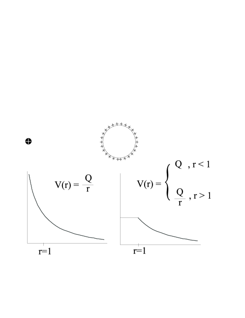
Figure 1: Electrostatic analogue of the patched flat-space–NS5-brane solution. The Coulomb potential of a point-like charge Q has a singularity at the origin, which is resolved if the same charge is distributed over the surface of a sphere (chosen here of unit radius). The Coulomb potential plays the role of the dilaton field and the charge is $N$.

Concerning the dilaton field, Neveu–Schwarz and Dirichlet sources lead to different pictures, according to Eqs. (6) and (15). For NS5-branes, the excised ball removes altogether the divergent-coupling region of the canonical neutral five-brane, and replaces it with a constant one, $g_{\rm s}^{2}=h_{0}^{\vphantom{2}}+N^{\vphantom{2}}$. In the case of D5-branes, the coupling inside the ball ($r<1$) becomes also constant, $g_{\rm s}^{2}=\left(h_{0}^{\vphantom{2}}+N^{\vphantom{2}}\right)^{-1}$. These results are summarized in Fig. 2.

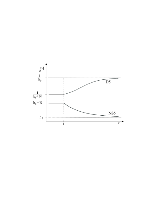
Figure 2: The string coupling of solution (15) is finite everywhere for the NS5-branes ($\gamma=+1$) and its electrostatic analogue is given in Fig. (1). However, it diverges when the sources are D5-branes and $h_{0}=0$.

As we have already stressed, a remarkable situation is provided by $h_{0}=0$. For negative $z$, the transverse space is flat, as for generic $h_{0}$. For positive $z$, the geometry is that of a three-sphere of radius $L=\sqrt{\alpha^{\prime}N}$ plus linear dilaton (see Eqs. (11) and (10)). Both patches are type-II string backgrounds described in terms of exact $N=4$ superconformal theories. In the case of Neveu–Schwarz sources, these are free of strong-coupling singularities.

4 Orbifold and orientifold planes

In fact, solution (15) is the only one that corresponds to a NS5-brane distribution, with a string coupling that remains finite everywhere. However, this solution fails to regularize the D5-brane configuration when the latter is singular, namely for $h_{0}=0$. Indeed, the string coupling is then divergent for large $z$, which is outside the excised ball. To ensure the finiteness of the coupling in the case at hand, we should instead consider a would-be dual solution:

$$h(z)=h_{0}+N\,{\rm e}^{-z+|z|},$$ (16)

and, by using (8),

$$f(z)=N\,\Theta(-z).$$ (17)

Flat space would be the geometry outside the three-sphere at $r=1$, whereas inside we would recover (9), that corresponds, for $h_{0}=0$, to the three-sphere plus linear-dilaton. Here, the coupling constant would be finite everywhere for $\gamma=-1$ (D5), while it would diverge at the origin ($z\to-\infty$) for $\gamma=+1$ (NS5).

The problem with (16) is that it does not solve Eq. (14), but solves a similar equation, with no negative sign (and $Z=0$). Such an equation can only be obtained by assuming $T_{5}<0$. We must therefore interpret solution (16) as resulting from $N$ remote branes ($z\to-\infty$ i.e. $r=0$), together with $N$ negative-tension objects localized at $z=0$ ($r=1$). The net effect of the latter is to screen the charge sitting at $r=0$ so as to ensure flat space for $r>1$. Again, this is the analogue of an electrostatic configuration, where a point-like charge is surrounded by a homogeneous spherical shell of opposite charge: outside the shell, the potential is constant whereas it is Coulomb inside.

The negative-tension objects under consideration are of two kinds: orientifold planes if they are associated with D-branes ($\gamma=-1$) or orbifold planes when they correspond to NS5-branes ($\gamma=+1$). They cannot have fluctuations in a unitary theory because the corresponding modes would be negative-norm.

5 Brane chains

At this stage of the paper, it has become clear that consistent string backgrounds can be constructed by using either five-branes or negative-tension objects. The dilaton depends on $\gamma$, but the geometry, which is governed by the function $h(z)$, does not (see Eqs. (2) and (4)–(6)). The function $h(z)$ depends, in turn, on whether the source is a brane or an orbifold/orientifold plane (for simplicity, we will call them generically “orbifold planes”, as long as we do not discriminate Neveu–Schwarz and Dirichlet, i.e. as long as we do not discuss the issue of the coupling but deal with the geometry only). The canonical solution (9) corresponds to a source made of $N$ branes pushed at $z\to-\infty$. In (15) those branes are at $z=0$, while solution (16) is generated by $N$ branes at $z\to-\infty$ together with $N$ orbifold planes located at $z=0$. One might wonder what would the solution look like in the case where both five-branes and five-orbifold planes are homogeneously distributed over the $S_{3}$ and localized at certain discrete values of the transverse coordinate $z$. In particular, one might also investigate the conditions under which the corresponding geometry is the target space of an exactly conformal sigma model. The aim of the present section is to clarify these issues.

The generalization of Eq. (14) for a network of sources reads (we have used the explicit expression for the d’Alembert operator):

$$h^{\prime\prime}+2h^{\prime}=-2\sum_{k=1}^{M}N_{k}\,\lambda_{k}\,{\rm e}^{-2z_{k}}\,\delta\left(z-z_{k}\right).$$ (18)

It describes the geometry generated by $N_{k}>0$ objects (five-branes or five-orbifold planes, depending on whether $\lambda_{k}=1$ or $-1$) located at $z=z_{k}$ for $k=1,\ldots,M$. One of the two integration constants of the above equation is the number of branes sitting at $z\to-\infty$, $N_{0}\geq 0$; those cannot be orbifold planes, that would generate negative $h(z)$, at least in the asymptotic region of negative $z$.

Between two consecutive stacks of branes, the solution of (18) is of the general type:

$$h(z)=h_{k}+\tilde{N}_{k}\,{\rm e}^{-2z},\ \ {\rm for}\ \ z_{k}\leq z\leq z_{k+1}\ \ k=0,\ldots,M$$ (19)

($z_{0}$ and $z_{M+1}$ are meant to be $-\infty$ and $+\infty$, respectively).

The “slopes” $\tilde{N}_{k}$ can be determined by computing the discontinuities of $h^{\prime}$ at the locations of the sources. Equation (18) enables us to write

$$\tilde{N}_{k}-\tilde{N}_{k-1}=\lambda_{k}\,N_{k}.$$ (20)

Put differently, $\tilde{N}_{k}$ is the integrated charge from $-\infty$ to $z_{k}$ included:

$$\tilde{N}_{k}=N_{0}+\sum_{i=1}^{k}\lambda_{i}\,N_{i}.$$

Continuity of $h(z)$, on the other hand, allows for the determination of the $h_{k}$’s:

$$h_{k-1}=h_{M}+\sum_{i=k}^{M}\lambda_{i}\,N_{i}\,{\rm e}^{-2z_{i}}\ \ k=1,\ldots,M,$$ (21)

where $h_{M}$ is the other integration constant.

The choice of the charges $N_{k}$ and of their positions $z_{k}$ is not completely arbitrary if one demands positivity of $h(z)$. In order to analyze this issue, we will focus on specific charge distributions where $\tilde{N}_{k}\geq 0\ \forall k$. Although this requirement is natural for $k=0$ in order to avoid $h(z)<0$ for negative enough $z$, we could in principle allow some negative integrated charges $\tilde{N}_{k}$ provided their positions as well as the integration constant $h_{M}$ are chosen in such a way that $h(z)$ remains positive everywhere. Our aim, however, is not to analyze the most general case, but situations which resemble (9), (15) and (16), where the total integrated charge is non-negative for any $z$. Moreover, as we will see later, backgrounds that can be described in terms of exact conformal theories turn out to belong to the class at hand.

Our claim is that if all localized charges $N_{k}$ are chosen in such a way that the integrated ones, $\tilde{N}_{k}$, are never negative, then $h(z)$ is non-negative, provided $h_{M}$ be non-negative, without any restriction on the positions $z_{k}$. Indeed, together with $\tilde{N}_{M}\geq 0$, $h_{M}\geq 0$ guarantees that $h(z)\geq 0$ when $z\gg z_{M}$. On the other hand, according to Eq. (19) and since $\tilde{N}_{k}\geq 0\ \forall k$, $h(z)$ is monotonically decreasing. So $h(z)$ is never negative.

The background described in Eq. (19) is not expected to be an exactly conformal model for generic values of the data $N_{k}$ and $z_{k}$. For every $k=0,\ldots,M$, a necessary condition is that either $h_{k}$ or $\tilde{N}_{k}$ vanishes. In the latter case, the space is flat, whereas in the former it contains a three-sphere plus a linear dilaton.

The starting point of our analysis is the recursion (continuity) relation

$$h_{k-1}=h_{k}+\lambda_{k}\,N_{k}\,{\rm e}^{-2z_{k}}$$

(this has led to (21)). By construction, $N_{k}>0$ for $k=1,\ldots,M$, while $N_{0}\geq 0$. Therefore, $h_{k}=0$ implies that $h_{k-1}=\lambda_{k}\,N_{k}\exp\left(-2z_{k}\right)\neq 0$. This result shows that it is impossible to have two consecutive domains in $z$, both with linear dilaton and three-sphere, separated by a distribution of five-branes. The only allowed pattern, compatible with exact CFT, is an alternation of flat-space and three-sphere-plus-linear-dilaton patches.

Hence, assuming that $h_{k}$ vanishes, we must impose $\tilde{N}_{k\pm 1}=0$, $h_{k\pm 2}=0$, etc. In particular, Eq. (20) now reads:

$$\tilde{N}_{k}=\lambda_{k}\,N_{k}=-\lambda_{k+1}\,N_{k+1}.$$ (22)

Under these circumstances, a necessary and sufficient condition for $h(z)$ to be non-negative is that $\tilde{N}_{k}>0$. This guarantees that $h(z)>0$ (i) for $z_{k-1}\leq z\leq z_{k}$, where $h(z)=h_{k-1}=\tilde{N}_{k}\exp\left(-2z_{k}\right)$; (ii) for $z_{k}\leq z\leq z_{k+1}$, where $h(z)=\tilde{N}_{k}\exp(-2z)$. From Eq. (22), we therefore learn that $\lambda_{k}=1=-\lambda_{k+1}$ and $N_{k}=N_{k+1}$. Suppose that $N_{k}$ five-branes are sitting at $z_{k}$ with a total integrated charge $\tilde{N}_{k}=N_{k}$. The function $h(z)$ is exponentially decreasing up to $z_{k+1}$, where $N_{k+1}=N_{k}$ five-orbifold planes are localized. The total integrated charge $\tilde{N}_{k+1}$ vanishes again, and $h(z)$ remains constant and equal to $h_{k+1}=N_{k+2}\exp\left(-2z_{k+2}\right)$ until $z_{k+2}$. Another stack of $N_{k+2}>N_{k}$ five-branes appear at that point and the process wraps back. Figure 3 depicts the situation.

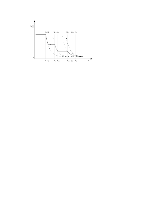
Figure 3: A partial sequence of five-branes (at $z_{k},z_{k\pm 2},\ldots$) and five-orbifold planes (at $z_{k\pm 1},z_{k\pm 3},\ldots$) appears in the center of this figure. The charges $\cdots<N_{k-2}<N_{k}<N_{k+2}<\cdots$ are independent data, together with $z_{k},z_{k\pm 2},\ldots$ The whole drawing is the solution (25).

At this stage, it is important to notice that not all $N_{k}$’s and $z_{k}$’s are independent parameters. We have already observed that only the charges of, say, the five-branes (i.e. those with $\lambda_{k}=1$) can be chosen arbitrarily; the charges of five-orbifold planes are then automatically determined. Moreover, given the positions of the five-branes, $z_{k},z_{k\pm 2},\ldots$, we determine those of the five-orbifold planes:

$$z_{k-1}=z_{k}-\frac{1}{2}\log\frac{N_{k}}{N_{k-2}},$$ (23)

This relation shows in particular that the two sets of parameters, the charges $\{N_{k}$, $N_{k\pm 2}$, $\ldots\}$ and the brane positions $\{z_{k},z_{k\pm 2},\ldots\}$, though independent, must obey the following conditions:

$$z_{k-2}<z_{k}-\frac{1}{2}\log\frac{N_{k}}{N_{k-2}}.$$ (24)

For practical purposes (see Section 7) it is useful to present the solution $h(z)$ corresponding to a set of data (charges and positions) in explicit and closed form. Let us suppose for concreteness that there is a no charge at $z\to-\infty$: $N_{0}=0$. Assuming an odd number of sources, $M=2L-1$, the independent data are chosen to be the charges of the five-branes $\{N_{1},N_{3},\ldots,N_{2L-1}\}$, with $\lambda_{2s+1}=1$, together with their positions $\{z_{1},z_{3},\ldots,z_{2L-1}\}$. The charges $N_{2s}$ and positions $z_{2s}$ of the five-orbifold planes ($\lambda_{2s}=-1$) are given respectively by Eqs. (22) and (23) with $k=2s+1$. Assuming that inequality (24) is fulfilled, $h(z)$ reads:

$$\begin{split}h(z)=&\sqrt{N_{1}\,N_{2L-1}}\exp\left(-(z+z_{1})-\left|z-z_{1}\right|\right)\times\\ &\times\prod_{s=1}^{L-1}\exp\left(\left|z-z_{2s+1}+\frac{1}{2}\log\frac{N_{2s+1}}{N_{2s-1}}\right|-\left|z-z_{2s+1}\right|\right).\end{split}$$ (25)

We are in the case where $h(z)$ does not diverge at $z\to-\infty$, and vanishes at $z\to+\infty$: $h(z\leq z_{1})=h_{0}=N_{1}\exp(-2z_{1})$ and $\lim_{z\to+\infty}h(z)=0$. The transverse space is flat for $z\leq z_{1}$ and has the geometry of a three-sphere plus linear dilaton for $z\geq z_{2L-1}$. This is a consequence of the absence of remote five-branes at $z\to-\infty$, and of the presence of $N_{2L-1}$ five-branes as last source. Figure 3 summarizes those features.

Any other situation can be obtained directly from Eq. (25), by considering appropriate limits. In the limit $z_{1}\to-\infty$, $N_{1}$ five-branes are pushed far away. The function $h(z)$ now diverges at $z\to-\infty$: for $z\leq z_{2}$ it describes a three-sphere plus linear dilaton. On the other hand, when $z_{2L-1}$ is sent to $+\infty$, the last sources are five-orbifold planes localized at $z=z_{2L-2}$. From this point $h(z)$ will be constant and the transverse space flat. Finally, both limits can be simultaneously taken, so that for $z\leq z_{2}$ and $z\geq z_{2L-2}$, the space becomes, respectively, a three-sphere plus a linear dilaton, and flat. This exhausts all the possibilities for constructing string backgrounds generated by five-branes and five-orbifold planes, that can be described in terms of exact CFT’s. All these constructions have natural electrostatic analogues, which consist of $M$ homocentric thin shells with charges alternating in sign, with or without a charge at the origin ($r=0$ i.e. $z\to-\infty$).

As far as the string coupling is concerned (see Eq. (6)), all possible situations appear: it might vanish, remain finite, or become infinite in one or both regions $r=0$ and $r\to\infty$, for either Dirichlet or Neveu–Schwarz five-brane backgrounds.

6 D5-NS5 transition in type-IIB theory

We have by now become familiar with the construction of elaborate configurations of stacks of branes uniformly distributed over homocentric three-spheres. As already stressed previously, the geometry (i.e. the metric) generated by such configurations does not depend on the nature of the five-branes/five-planes which are present. The dilaton, however, does: the string coupling, $\exp 2\phi$, is equal to $h(r)$ or $h(r)^{-1}$ for NS–NS or R–R backgrounds, respectively (see Eqs. (2) and (4)–(6)). If we try therefore to repeat the analysis of Section 5 for type-IIB backgrounds whit both NS5-branes and D5-branes (together with their negative-tension counterparts), we will generically face discontinuities in the dilaton field at the location of the source-shells. Alternatively, continuity requirement for the dilaton leads to discontinuities in $h$, which amount to $\delta$-function terms in the three-form field strength.

There is, however, one instance, where a continuous interpolation between NS5-brane and D5-brane backgrounds is possible. In the type-IIB theory, D5- and NS5-branes are S-dual. If two distinct regions of space–time, hosting NS–NS and R–R backgrounds respectively, are due to be smoothly patched together, this must happen at the S-self-dual point.

Let us be more concrete and consider $N$ D5-branes sitting at $r=0$. For $0<r\leq r_{\rm S}$ those create a three-sphere (transverse) geometry plus (finite) linear dilaton and R–R antisymmetric tensor (Eqs. (6) and (9) with $\gamma=-1$ and $h_{0}=0$). At radius $r=r_{\rm S}$, we introduce a set of $N$ orientifold five-planes, uniformly distributed, together with $N$ NS5-branes – put differently, a O–NS bound-state. The R–R charge is therefore screened, so that the R–R antisymmetric tensor vanishes for $r\geq r_{\rm S}$, while a NS–NS one is switched on.

From the geometry point of view, the presence of the O–NS bound-state distribution is transparent:

$$h(r)=\frac{N}{r^{2}},$$

everywhere, which ensures the $S^{3}$ factor. As already stressed, this distribution alters the dilaton field:

$$\,{\rm e}^{2\phi}=\left\{\begin{array}[]{lll}\displaystyle{r^{2}\over N},&\phantom{aa}&0<r\leq r_{\rm S},\\ \\ \frac{\displaystyle N}{\displaystyle r^{2}},&\phantom{aa}&r_{\rm S}\leq r.\end{array}\right.$$

Continuity of the latter demands the parameter $r_{\rm S}$ be the S-self-dual point, namely

$$h(r_{\rm S})=\frac{1}{h(r_{\rm S})}.$$

This implies $r_{\rm S}=\sqrt{N}$.

The antisymmetric tensors are discontinuous at $r=\sqrt{N}$. Inside we have the R–R background of the D5-brane which is zero outside, and vice versa for the NS–NS background. Notice that the source action to be added to the bulk action is in this case

$$\begin{split}S_{\rm O-NS}=&\frac{N\,T_{5}}{2\pi^{2}}\int d^{10}x\,\sin^{2}\!\theta\,\sin\varphi\,\delta(r-\sqrt{N})\left(\,{\rm e}^{{1\over 2}\phi}\sqrt{-\hat{g}^{(6)}}+\tilde{B}_{6}\right)\\ -&\frac{N\,T_{5}}{2\pi^{2}}\int d^{10}x\,\sin^{2}\!\theta\,\sin\varphi\,\delta(r-\sqrt{N})\left(\,{\rm e}^{-{1\over 2}\phi}\sqrt{-\hat{g}^{(6)}}+\tilde{C}_{6}\right).\end{split}$$

In the above configuration, the coupling is small everywhere except near $r=\sqrt{N}$, where it is of order one. This is the price to pay for continuously interpolating between NS–NS and R–R backgrounds. We could excise the order-one-coupling region, by separating the O5-plane and NS5-brane shells. This amounts, however, to abandon the continuity requirement. We will not pursue any further this issue.

7 Gravitational fluctuations

In this section, we consider gravitational fluctuations of the five-brane solutions derived in Sections 4 and 5. Our motivation is to analyze the low-lying spectrum of states, which can be eventually compared with exact CFT results, available in the present setting [31]. Furthermore, this analysis is important for clarifying the issue of localization of the states in the vicinity of the branes. Our conclusion is that in the framework of the five-brane and five-orbifold backgrounds presented so far, gravitons and their K–K descendants have a mass gap in accordance with the CFT analysis, [1, 10, 11, 31]. Other fluctuations (Neveu–Schwarz, Ramond–Ramond, …) can be studied in the same manner, but this is beyond the scope of the present work.

We will restrict ourselves to gravitational fluctuations that are longitudinal to the brane. To this end we consider small perturbations of the background metric (2), (4) and (5), of the form

$$ds^{2}=\alpha^{\prime}\,h(r)^{-\frac{1}{4}}\left(\eta_{ij}+\rho_{ij}\right)\,dx^{i}\,dx^{j}+\alpha^{\prime}\,h(r)^{\frac{3}{4}}\left(dr^{2}+r^{2}d\Omega_{3}^{2}\right),$$ (26)

where $\{x^{i},i=0,\ldots,5\}=\{t,\vec{x}\}=x$. The linearized Einstein equations in the transverse, traceless gauge, $\rho^{i}_{\,i}=\partial^{i}\rho_{ij}=0$, taking also into account the sources, reduce to the covariant scalar equation [23, 33]:

$$\large\hbox{{$\sqcup$}\hbox to0.0pt{\hss$\sqcap$}}\rho_{ij}=0,$$ (27)

where the d’Alembert operator is that of the unperturbed metric. The solutions of the above equation belong to the gravitational K–K sector. Considering a K–K mode with mass $M$ ($M^{2}$ is measured in units of $1/\alpha^{\prime}$), and assuming the factorization $\rho_{ij}\left(x,r,\Omega\right)=\tilde{\rho}_{ij}\left(x\right)\,\phi(r,\Omega)$, with $\large\hbox{{$\sqcup$}\hbox to0.0pt{\hss$\sqcap$}}_{6}\tilde{\rho}_{km}\equiv\eta^{ij}\partial_{i}\partial_{j}\tilde{\rho}_{km}=M^{2}\tilde{\rho}_{km}$, Eq. (27) reduces to its transverse part

$$\left(\frac{1}{r^{3}}\partial_{r}r^{3}\partial_{r}+\frac{1}{r^{2}}\triangle_{S^{3}}+M^{2}\,h(r)\right)\phi(r,\Omega)=0,$$ (28)

where $\Delta_{S^{3}}$ is the Laplacian operator on the three-sphere. We can further decompose the transverse-space dependence of the fluctuations: $\phi(r,\Omega)=r^{-3/2}\,y_{\ell}(r)\,D^{\ell}_{nn^{\prime}}(\Omega)$, where $D^{\ell}_{nn^{\prime}}(\Omega)$ form a complete set of orthonormal functions on $S^{3}$:

$$\triangle_{S^{3}}D^{\ell}_{nn^{\prime}}(\Omega)=-\ell(\ell+2)D^{\ell}_{nn^{\prime}}(\Omega).$$

Then the radial equation reads:

$$\left[-\frac{d^{2}}{dr^{2}}+\frac{1}{r^{2}}\left(\ell+\frac{1}{2}\right)\left(\ell+\frac{3}{2}\right)\right]\,y_{\ell}(r)=M^{2}\,h(r)\,y_{\ell}(r),$$ (29)

which is a the Sturm–Liouville equation.

The natural inner product for the radial wave functions $y_{\ell}(r)$ is obtained by analyzing the normalization of the kinetic terms for $\rho_{ij}$ as they appear when the fluctuations $g_{ij}=\eta_{ij}+\rho_{ij}$ are introduced in the action (Eqs. (1) and (12)), and the latter is expanded. We obtain:

$$\parallel y_{\ell}\parallel^{2}=\int_{0}^{\infty}dr\,h(r)\,y_{\ell}(r)^{2}.$$ (30)

With this precise inner product, the Sturm–Liouville operator (in the square brackets of the lhs of (29)) is self-adjoint, provided some appropriate boundary conditions are imposed, which include those we will consider here: $y_{\ell}(0)=0$ and $\lim_{r\to\infty}y_{\ell}^{\prime}(r)=0$. This property ensures the existence of a complete set of orthonormal eigenfunctions, whose $M^{2}$-spectrum is real, non-degenerate, bounded from bellow, and contains at least a continuous part.

In order to determine the spectrum we need a specific background. We will consider for simplicity the single five-brane shell solution (15) with $h_{0}=0$:

$$h(r)=\left\{\begin{array}[]{ll}\displaystyle{N\over R^{2}},&0\leq r\leq R,\\ \\ \frac{\displaystyle N}{\displaystyle r^{2}},&R\leq r.\end{array}\right.$$ (31)

The eigenfunctions of (29) are obtained by following the standard strategy. We first solve Eq. (29) for $0\leq r\leq R$ and keep only solutions that satisfy $y_{\ell}(0)=0$. For $M^{2}\neq 0$, those are Bessel functions

$$y_{\ell}(r)=A_{\ell}\,\sqrt{r}\,J_{\ell+1}\left({M\sqrt{N}r\over R}\right),\ \ 0\leq r\leq R,$$ (32)

behaving like $r^{\ell+3/2}$ in the vicinity of $r=0$; $A_{\ell}$ is an arbitrary, real constant. This solution holds even for $M^{2}<0$ (in that case $A_{\ell}$ is a real number times $i^{-(\ell+1)}$). Notice that $\sqrt{r}N_{\ell+1}\left(M\sqrt{N}r/R\right)$ is also a solution, which must be discarded because of its bad behavior ($r^{-\ell-1/2}$) at the origin. For $M^{2}=0$, the only acceptable solution is

$$y_{\ell}(r)=A_{\ell}\,\sqrt{r}\left({r\over R}\right)^{\ell+1},\ \ 0\leq r\leq R,\ \ M^{2}=0.$$

We must now solve Eq. (29) for $r\geq R$. Depending on $\ell$ and $M$, the behavior is either oscillatory or power-law:

$$y_{\ell}(r)=B_{\ell}\,\sqrt{r}\,\cos\left(\sqrt{M^{2}N-(\ell+1)^{2}}\log\left({r\over R}\right)+\Phi_{\ell}\right)\ ,\ \ M^{2}\geq\frac{(\ell+1)^{2}}{N},$$ (33)

where $B_{\ell}$ and $\Phi_{\ell}$ are arbitrary, real constants, and

$$y_{\ell}^{\vphantom{+}}(r)=\sqrt{r}\left(C_{\ell}^{-}\left(\frac{R}{r}\right)^{\left((\ell+1)^{2}-M^{2}N\right)^{1/2}}+C_{\ell}^{+}\left(\frac{r}{R}\right)^{\left((\ell+1)^{2}-M^{2}N\right)^{1/2}}\right)\ ,\ \ M^{2}\leq\frac{(\ell+1)^{2}}{N}.$$ (34)

The latter holds even for $M^{2}\leq 0$, and $C_{\ell}^{\pm}$ are again real and arbitrary. In fact, we must set $C_{\ell}^{+}$ to zero, because with the inner product (30) and (31), $r^{1/2+\sqrt{(\ell+1)^{2}-M^{2}N}}$ is not even $\delta$-function normalizable. However, $r^{1/2-\sqrt{(\ell+1)^{2}-M^{2}N}}$ is normalizable, while (33) is $\delta$-function normalizable (both satisfy the previously advertised boundary condition at infinity). The spectrum is therefore expected to be continuous for $M^{2}N\geq(\ell+1)^{2}$ and discrete otherwise.

The complete determination of the eigenfunctions is achieved by requiring continuity at $r=R$. On one hand, continuity of $y_{\ell}$ fixes $B_{\ell}^{\vphantom{-}}$ or $C_{\ell}^{-}$ in terms of $A_{\ell}^{\vphantom{-}}$, leaving only an overall free normalization. Continuity of the logarithmic derivative, on the other hand, allows for the computation of the phase $\Phi_{\ell}$ if $M^{2}\geq{(\ell+1)^{2}}/{N}$ (continuous spectrum), and the positions of the discrete mass levels if $M^{2}\leq{(\ell+1)^{2}}/{N}$. We find

$$\Phi_{\ell}=-{\rm arctan\,}\left(\frac{1}{\sqrt{1-(\ell+1)^{2}/M^{2}N}}\frac{J^{\prime}_{\ell+1}\left(M\sqrt{N}\right)}{J_{\ell+1}\left(M\sqrt{N}\right)}\right)$$

for the continuous spectrum, while the discrete spectrum turns out to be empty: no mass-squared levels (positive, zero or negative) exist for $M^{2}<{(\ell+1)^{2}}/{N}$. We therefore conclude that there is a mass gap $M_{\rm gap}=1/\sqrt{N}$ (in units of $M_{\rm s}$) in agreement with CFT [1, 10, 11, 31]. Choosing $B_{\ell}=\left(N-(\ell+1)^{2}/M^{2}\right)^{-1/4}$, the corresponding (complete) set of eigenfunctions is normalized as

$$\left(y_{\ell}^{(1)},y_{\ell}^{(2)}\right)=\frac{\pi}{2}\,\delta\left(M^{(1)}-M^{(2)}\right),$$

according to the inner product (30). For different $\ell$’s, orthogonality is guaranteed by the spherical functions $D^{\ell}_{nn^{\prime}}$.

Our result deserves several comments. First, had we considered instead of (31) a more general conformal background of the type (25), our conclusions would not have been modified. For $0\leq r\leq r_{1}\equiv\exp z_{1}$ we have indeed the solution (32) with $N$ replaced with $N_{1}/r_{1}^{2}$, while (33) and (34) – with $C_{\ell}^{+}=0$ – are valid for $r\geq r_{2L-1}$ with $N_{2L-1}$ instead of $N$. Continuity constraints for $y_{\ell}(r)$ and $y_{\ell}^{\prime}(r)$ propagate through all intermediate-brane positions, determine completely the intermediate solutions, and eventually the spectrum of longitudinal gravitational fluctuations: this is a continuous spectrum above a mass gap $M_{\rm gap}=1/\sqrt{N_{2L-1}}$.

8 Holography

The framework is here the NS5-brane of type-IIA string theory. The non-normalizable modes in this background are expected to correspond, via the holographic principle [6, 12, 13], to off-shell operators of the decoupled world-volume theory of the five-brane. The boundary is at $r=R_{\infty}\to\infty$.

In the case under study, however, the identification of the radial direction as a renormalization-group flow is less clear. The space-time metric (in the string frame),

$$ds^{2}_{\sigma}={\alpha^{\prime}}\,dx^{2}_{\vphantom{3}}+{\alpha^{\prime}}\,h(r)\left(dr^{2}_{\vphantom{3}}+r^{2}_{\vphantom{3}}d\Omega_{3}^{2}\right),$$

is invariant under a rescaling of $r$. The only effect is to shift appropriately the position of the shell. If the shell is at the origin the metric is strictly invariant. The string coupling on the other hand $g_{\rm s}^{2}=\,{\rm e}^{2\phi}=h(r)$ scales to zero as we approach the boundary.

The decoupling limit is [12]

$$g_{\rm s}=\,{\rm e}^{\phi}\to 0\ ,\ \ \ell_{\rm s}=\sqrt{\alpha^{\prime}}\ \ {\rm and}\ \ U={r\over g_{\rm s}\ell_{\rm s}}\ \ {\rm fixed,}$$

where $U$ is the tension of a D2-brane stretched between NS5-branes. It is the tension of a world-volume string and corresponds to a Higgs vev of the LST (boundary theory). Thus, the boundary theory has no dimensionless coupling constant and its scale is set by $\ell_{\rm s}$. The dilaton is given by $\,{\rm e}^{2\phi}={N\over U_{\vphantom{s}}^{2}\ell_{\rm s}^{2}}$, and vanishes at infinity. Using the relation between $r$ and energy ($U$), this implies that the region of small $r$ corresponds to the infra-red conformal theory.

The presence of the shell at $r=R$, modifies somewhat the picture above. First we choose the position of the shell (we will from now on rescale $r\to g_{\rm s}r$) so that $R\gg\sqrt{N}$. Large $N$ implies that all curvatures are small everywhere (so that stringy corrections can be neglected). In particular, the supergravity description is good at length scales larger than the string scale $\ell_{\rm s}$. The condition on $R$ also implies that the string coupling in the bulk is small everywhere. Thus, the supergravity description is reliable on the whole space.

In the background under consideration, the world-volume theory undergoes a Higgs phenomenon at an energy scale ${1\over\ell_{\rm s}R}$. Since $R\gg\sqrt{N}$ this has modified the effective field theory at lower scales. Below this scale, the coupling no longer runs.

There is another approximation that is relevant here, and this has to do with the continuous distribution of five-branes on the shell. String theory implies that the NS5-charge is quantized. Thus, if the source at $R$ is composed of $N$ NS5-branes, the distribution is quasi-continuous. In fact, the average distance (in transverse space) between the $N$ five-branes distributed over the sphere is $L\simeq N^{-1/3}\ell_{\rm s}R\gg N^{1/6}\ell_{\rm s}$. Thus, at large $N$, $L$ is much larger than the string scale but much smaller that the characteristic scale $\sqrt{N}\ell_{\rm s}$ of the world-volume theory.

We can summarize the previous discussion as follows: the supergravity description with $SO(4)$ symmetry is valid at length scales larger than $N^{1/6}\ell_{\rm s}$. At length scales larger than $\sqrt{N}\ell_{\rm s}$ the LST can be replaced by an effective field theory. At length scales smaller than $N^{1/6}\ell_{\rm s}$ but larger than $\ell_{\rm s}$ the supergravity description is valid but $SO(4)$ symmetry is broken.

We will now proceed to apply the holographic principle as implemented in [34] and calculate boundary correlators. In particular, we will focus on the (descendants) of the six-dimensional graviton, itself dual to the world-volume stress tensor. We have shown that the six-dimensional graviton ($\ell=0$)-fluctuation and its K–K descendants ($\ell>0$) satisfy Eq. (27) that can be recast in the form (28) or (29). For a given set of boundary data, $\bar{\rho}_{ij}^{\ell nn^{\prime}}(x,\Omega)=\bar{\rho}_{ij}^{\ell}(x)\,D^{\ell}_{nn^{\prime}}(\Omega)$, the corresponding partial-wave bulk solution, $\rho_{ij}^{\ell nn^{\prime}}(x,r,\Omega)=\rho_{ij}^{\ell}(x,r)\,D^{\ell}_{nn^{\prime}}(\Omega)$, can be expressed in terms of the bulk-to-boundary propagator $G_{\ell nn^{\prime}}(x,r,\Omega)=G_{\ell}(x,r)\,D_{nn^{\prime}}^{\ell}(\Omega)$:

$$\rho_{ij}^{\ell}(x,r)=\int d^{6}x^{\prime}\,G_{\ell}(x-x^{\prime},r)\,\bar{\rho}_{ij}^{\ell}(x^{\prime}).$$ (35)

The radial part of the above propagator satisfies

$$\left(\frac{1}{r^{3}}\partial_{r}r^{3}\partial_{r}-\frac{\ell(\ell+2)}{r^{2}}+h(r)\,\large\hbox{{$\sqcup$}\hbox to0.0pt{\hss$\sqcap$}}_{6}\right)G_{\ell}(x,r)=0$$ (36)

with the boundary condition

$$\lim_{r\to R_{\infty}}G_{\ell}(x,r)=\delta^{(6)}(x).$$

We will work from now on in Euclidean space, and Fourier transform the six-dimensional part

$$G_{\ell}(x,r)={1\over{\alpha^{\prime}}^{3}}\int{d^{6}p\over(2\pi)^{6}}\,{\rm e}^{ip\cdot x}\,G_{\ell}(p,r),$$

so that Eq. (36) becomes:

$$\left(\frac{1}{r^{3}}\partial_{r}r^{3}\partial_{r}-\frac{\ell(\ell+2)}{r^{2}}-h(r)\,p^{2}\right)G_{\ell}(p,r)=0$$ (37)

with boundary condition

$$\lim_{r\to R_{\infty}}G_{\ell}(p,r)=1.$$ (38)

The regular solution to the bulk equation (Eq. (37)) is

$$G_{\ell}(p,r)=\left\{\begin{array}[]{ll}\displaystyle{A_{\ell}(p)\over r}\,I_{\ell+1}\left(\displaystyle{\sqrt{p^{2}N}r\over R}\right),\hfill 0\leq r\leq&R,\\ \\ \displaystyle{C^{-}_{\ell}(p)\over r}\left(\displaystyle{R\over r}\right)^{\sqrt{(\ell+1)^{2}+p^{2}N}}+\displaystyle{C^{+}_{\ell}(p)\over r}\left(\displaystyle{r\over R}\right)^{\sqrt{(\ell+1)^{2}+p^{2}N}},\ R\leq&r.\end{array}\right.$$ (39)

The boundary condition (38) is satisfied provided

$${C^{+}_{\ell}(p)\over R_{\infty}}=\left({R\over R_{\infty}}\right)^{\sqrt{(\ell+1)^{2}+p^{2}N}}.$$

The rest of the coefficients are determined from the usual matching conditions (continuity of the propagator and its logarithmic derivative). We obtain:

$${A_{\ell}(p)\over R_{\infty}}=\left({R\over R_{\infty}}\right)^{\sqrt{(\ell+1)^{2}+p^{2}N}}{2\sqrt{(\ell+1)^{2}+p^{2}N}\over\sqrt{(\ell+1)^{2}+p^{2}N}\,I_{\ell+1}\left(\sqrt{p^{2}N}\right)+\sqrt{p^{2}N}\,I^{\prime}_{\ell+1}\left(\sqrt{p^{2}N}\right)}$$

and

$${C^{-}_{\ell}(p)\over R_{\infty}}=\left({R\over R_{\infty}}\right)^{\sqrt{(\ell+1)^{2}+p^{2}N}}{\sqrt{(\ell+1)^{2}+p^{2}N}\,I_{\ell+1}\left(\sqrt{p^{2}N}\right)-\sqrt{p^{2}N}\,I^{\prime}_{\ell+1}\left(\sqrt{p^{2}N}\right)\over\sqrt{(\ell+1)^{2}+p^{2}N}\,I_{\ell+1}\left(\sqrt{p^{2}N}\right)+\sqrt{p^{2}N}\,I^{\prime}_{\ell+1}\left(\sqrt{p^{2}N}\right)}.$$

In order to make contact with holography, we would like to analyze the dynamics of the six-dimensional gravitational perturbations $\rho_{ij}(x^{\mu})$ considered in (26), from a slightly different point of view. Let us write down the linearized action for those fields, as it appears when expression (26) is plugged into Eq. (1). We obtain (in the transverse, traceless gauge considered so far):

$$S_{2}={3{\alpha^{\prime}}^{4}\over 2\kappa_{10}^{2}}\int d^{6}x\,d^{4}y\left(h\,\partial^{i}\rho_{jk}\,\partial_{i}\rho^{jk}+\partial^{a}\rho_{jk}\,\partial_{a}\rho^{jk}\right),$$

where $\{y^{a},a=6,\ldots,9\}$ are transverse coordinates such that $dr^{2}+r^{2}d\Omega_{3}^{2}=\sum_{a}(dy^{a})^{2}$ with $\sum_{a}(y^{a})^{2}=r^{2}$. The Gibbons–Hawking boundary term, the antisymmetric-tensor and dilaton terms, as well as the source term vanish. By using the partial-wave expansion of $\rho_{ij}(x^{\mu})$, integration by parts, ortho-normality relations for the $D^{\ell}_{nn^{\prime}}(\Omega)$, equations of motion, as well as Eq. (35) and the above expressions for the bulk-to-boundary propagator (see Eq. (39)), we can expand $S_{2}$ in partial waves,

$$S_{2}^{\phantom{\ell}}=\sum_{\ell=0}^{\infty}S_{2}^{\ell},$$

and determine $S_{2}^{\ell}$ in terms of the Fourier-transformed boundary data $\bar{\rho}^{\ell}_{ij}(p)$:

$$S_{2}^{\ell}=-{3\over 2\kappa_{10}^{2}{\alpha^{\prime}}^{2}}\int d^{6}p\,\bar{\rho}_{ij}^{\ell}(p)\,\bar{\rho}^{\ell ij}(-p)\,R_{\infty}^{2}\,\Upsilon_{\ell}.$$

We have introduced the function

$$\begin{split}\Upsilon_{\ell}(p)=&\left(1-\sqrt{(\ell+1)^{2}+p^{2}N}\right)+2\chi_{\ell}\left({R\over R_{\infty}}\right)^{2\left((\ell+1)^{2}+p^{2}N\right)^{1/2}}\\ &+\chi_{\ell}^{2}\left(1+\sqrt{(\ell+1)^{2}+p^{2}N}\right)\left({R\over R_{\infty}}\right)^{4\left((\ell+1)^{2}+p^{2}N\right)^{1/2}},\end{split}$$

where $\chi_{l}$ also depends on $p^{2}N$

$$\chi_{\ell}(p)={\sqrt{(\ell+1)^{2}+p^{2}N}\,I_{\ell+1}\left(\sqrt{p^{2}N}\right)-\sqrt{p^{2}N}\,I^{\prime}_{\ell+1}\left(\sqrt{p^{2}N}\right)\over\sqrt{(\ell+1)^{2}+p^{2}N}\,I_{\ell+1}\left(\sqrt{p^{2}N}\right)+\sqrt{p^{2}N}\,I^{\prime}_{\ell+1}\left(\sqrt{p^{2}N}\right)}$$

with the following asymptotic behavior:

$$\chi_{\ell}(p)={2\ell^{2}+9\ell+11\over 8(\ell+1)^{2}\,(\ell+2)\,(\ell+3)}\,p^{2}N+{\cal O}\left(p^{4}N^{2}\right)\ ,\ \ Np^{2}\ll 1,$$

while

$$\chi_{\ell}={1\over 4\sqrt{p^{2}N}}+{\cal O}\left({1\over p^{2}N}\right)\ ,\ \ Np^{2}\gg(\ell+1)^{2}.$$

Thus, $\chi_{\ell}$ vanishes at $p\to 0$ and $p\to\infty$, and has a maximum at $\sqrt{p^{2}N}\sim\ell+1$.

We should note that the three different terms have different asymptotic behavior as the renormalization screen moves to infinity ($R_{\infty}\to\infty$), with the first term giving the leading contribution. In the region of validity of the supergravity approximation, $p^{2}N$ can be either very small or very large, (the first region corresponds to the effective-field-theory region, while the second to the LST region), so $\sqrt{(\ell+1)^{2}+p^{2}N}$ cannot be expanded in a sequence of local terms. Thus, if we insist on keeping the stringy physics of LST, we must renormalize $\bar{\rho}_{ij}^{\ell}\to{\alpha^{\prime}}^{-1/2}R_{\infty}^{-1}\bar{\rho}_{ij}^{\ell}$, in which case the terms proportional to $\chi_{\ell}$ and $\chi_{\ell}^{2}$ vanish in the $R_{\infty}\to\infty$ limit with the result:

$$S_{2}^{\ell}=-{3\over 2\kappa_{10}^{2}{\alpha^{\prime}}^{3}}\int d^{6}p\,\bar{\rho}_{ij}^{\ell}(p)\,\bar{\rho}^{\ell ij}(-p)\left(-1+\sqrt{(\ell+1)^{2}+p^{2}N}\right).$$ (40)

At this point we can take advantage of the transverse-tracelessness conditions, which in momentum space read $\rho_{i}^{i}=p^{i}\rho_{ij}=0$, to “covariantize” the two-point correlator appearing in Eq. (40):

$$S_{2}^{\ell}=-{3\over 4\kappa_{10}^{2}{\alpha^{\prime}}^{3}}\int d^{6}p\,\bar{\rho}_{ij}^{\ell}(p)\,\bar{\rho}_{km}^{\ell}(-p)\,F_{\ell}^{ij;km}(p)$$

with

$$F_{\ell}^{ij;km}(p)=\left(\pi^{ik}\,\pi^{jm}+\pi^{im}\,\pi^{jk}-{2\over 5}\,\pi^{ij}\,\pi^{km}\right)\left(-1+\sqrt{(\ell+1)^{2}+p^{2}N}\right),$$

where

$$\pi^{ij}=\delta^{ij}-{p^{i}\,p^{j}\over p^{2}}$$

are the projectors that impose conservation of the boundary stress tensor and its K–K descendants. Thus, we expect that

$$\left\langle T_{\ell}^{ij}(p)\,T_{\ell^{\prime}}^{km}(-p)\right\rangle=-{3\over 4\kappa_{10}^{2}{\alpha^{\prime}}^{3}}\,F_{\ell}^{ij;km}(p)\,\delta_{\ell\ell^{\prime}},$$ (41)

which is compatible with conservation and tracelessness of the stress tensor and its cousins. Notice that the two-point function is insensitive to the presence of the shell. This will no longer be true for higher correlators.

Fourier transforming in configuration space we obtain:

$$\left\langle T_{\ell}^{ij}(x)\,T_{\ell}^{km}(0)\right\rangle=\left(\hat{\pi}^{ik}\,\hat{\pi}^{jm}+\hat{\pi}^{im}\,\hat{\pi}^{jk}-{2\over 5}\hat{\pi}^{ij}\,\hat{\pi}^{km}\right)F_{\ell}(x)$$

with

$$F_{\ell}(x)=-{3\over 4\kappa_{10}^{2}{\alpha^{\prime}}^{3}}\int d^{6}p\,\,{\rm e}^{ip\cdot x}\left(-1+\sqrt{(\ell+1)^{2}+p^{2}N}\right)$$

and

$$\hat{\pi}^{ij}=\delta^{ij}-{\partial^{i}\,\partial^{j}\over\large\hbox{{$\sqcup$}\hbox to0.0pt{\hss$\sqcap$}}_{6}}.$$

It is instructive here to pause and calculate the canonical dimension of $T^{ij}_{\ell}(p)$. For this we need to remember that $\bar{\rho}_{ij}^{\ell}(x)$ has canonical mass dimension zero, and its Fourier transform $\bar{\rho}_{ij}^{\ell}(p)$ mass dimension $-6$. For renormalization purposes we have absorbed a factor of $\sqrt{\alpha^{\prime}}R_{\infty}$ in it so its canonical dimension changed to $-7$. Thus, the canonical mass dimension of $T^{ij}_{\ell}(p)$ is $+7$. This is reflected in (41), taking into account that $\kappa_{10}$ has dimension $-4$.

We can evaluate the Fourier transform by using the following formula:

$$\begin{split}-1+\sqrt{(\ell+1)^{2}+p^{2}N}=&{1\over\sqrt{\pi}}\int_{(\ell+1)^{2}+p^{2}N}^{1}dz\,\int_{0}^{\infty}du~{}\,{\rm e}^{-zu^{2}}\\ =&{1\over\sqrt{\pi}}\int_{0}^{\infty}{du\over u^{2}}\left(\,{\rm e}^{-u^{2}\left((\ell+1)^{2}+p^{2}N\right)}-\,{\rm e}^{-u^{2}}\right).\end{split}$$

Assuming $|x|\not=0$, and expressing $\kappa_{10}$ and $\alpha^{\prime}$ in terms of $M_{\rm s}$, we obtain the result:

$$F_{\ell}(x) = -{3\over 2(2\pi)^{4}}{M_{\rm s}^{14}\over|x|^{7}}\,\,{\rm e}^{-{(\ell+1)|x|\over\sqrt{N}}}\times$$

$$\times\left(15+15\,{(\ell+1)|x|\over\sqrt{N}}+6\left({(\ell+1)|x|\over\sqrt{N}}\right)^{2}+\left({(\ell+1)|x|\over\sqrt{N}}\right)^{3}\right).$$

Note that for the modes with $\ell\not=0$, there is a contact term proportional to a $\delta$-function at $x=0$.

The above result implies that at large distances the effective mass is $M_{\rm eff}={(\ell+1)\over\sqrt{N}}$. This is the same as the mass gap we found for the normalizable modes (previous section). We also observe that the “stringy” two-point function is independent of the presence of the shell. This is not true for higher correlators because those involve the bulk-to-bulk propagator (which is computed in the appendix) and depend on the presence of the shell. A direct calculation (up to projectors) gives:

$$F_{3}(p_{1},p_{2},p_{3}) \sim \lim_{R_{\infty}\to\infty}\int_{0}^{\infty}dr\,G_{\ell_{1}}(p_{1},R_{\infty})\,G_{\ell}(p_{2},r)\,G_{\ell}(p_{3},r)\,B_{\ell_{1}}(p_{2}+p_{3},R_{\infty};r)\times$$

$$\times\delta(p_{1}+p_{2}+p_{3}),$$

and the result depends on the position of the shell via the bulk-to-bulk propagator $B_{\ell}(p,R_{\infty};r)$.

If, however, we restrict ourselves to the effective-field-theory region $\sqrt{p^{2}N}\ll 1$, we can expand the square root in a power series in $p^{2}N$, keeping the first few terms. Such terms can be removed by local counterterms, and the renormalized boundary data become

$$\bar{\rho}^{\ell}_{{\rm ren},ij}(p)=\left({R_{\infty}\over R}\right)^{-\ell-{p^{2}N\over 2(\ell+1)}}\bar{\rho}^{\ell}_{ij}(p).$$

We find

$$F_{\ell}^{ij;km}(p)=\left(\pi^{ik}\,\pi^{jm}+\pi^{im}\,\pi^{jk}-{2\over 5}\pi^{ij}\,\pi^{km}\right){2R^{2}\,\chi_{\ell}(p)}.$$

This correlator is analytic in the infra-red. Thus, the presence of the shell seems to completely break the conformal symmetry.

9 The spectrum of massless localized states

In this section we will investigate the spectrum of massless states localized on the brane distribution at $r=R$. The correct but tedious procedure is to study in detail the fluctuations of the background solution including the $\delta$-function sources. We will however take here a short-cut due to the fact that the background configuration is BPS, and the massless fluctuations are constrained by lack-of-force condition and supersymmetry. They correspond therefore to deformations of the brane distribution plus supersymmetric patterns.

It is therefore enough to consider the background “BPS condition”, Eq. (14):

$$\large\hbox{{$\sqcup$}\hbox to0.0pt{\hss$\sqcap$}}_{4}h=-2{N\over R^{3}}\,\delta(r-R),$$

where we have assumed that $h$ may depend in general on all four transverse coordinates $\{y^{a},a=6,\ldots,9\}\equiv\{r,\Omega\}$ ($\large\hbox{{$\sqcup$}\hbox to0.0pt{\hss$\sqcap$}}_{4}$ is the corresponding “flat” Laplacian introduced previously). Our aim is to go beyond the spherical solution of $N$ five-branes, Eq. (31). Perturbations of this solution involve deformations of the shell as well as of the charge density, keeping the total charge fixed. Thus, the equation for the small fluctuations is

$$\large\hbox{{$\sqcup$}\hbox to0.0pt{\hss$\sqcap$}}_{4}(h+\delta h)=-4\pi^{2}\left(\varrho_{0}+\delta\varrho(\Omega)\right)\delta(r-R+\delta f(\Omega)),$$ (42)

where $\varrho_{0}={N\over 2\pi^{2}R^{3}}$ is the unperturbed constant density of five-branes over the three-sphere, and $\delta\varrho(\Omega)$ and $\delta f(\Omega)$ small perturbations of the density and shape of the distribution. Expanding Eq. (42) to first order we obtain:

$$\large\hbox{{$\sqcup$}\hbox to0.0pt{\hss$\sqcap$}}_{4}\delta h=-4\pi^{2}\delta\varrho(\Omega)\,\delta(r-R)-4\pi^{2}\varrho_{0}\,\delta f(\Omega)\,\delta^{\prime}(r-R).$$ (43)

In the rest of this section, we will try to get a flavor of the massless spectrum as it comes out of Eq. (43). Let us expand the various functions in $SU(2)$ spherical harmonics:

$$\delta h(r,\Omega) = \sum_{\ell,n,n^{\prime}}h_{\ell}^{n,n^{\prime}}(r)\,D^{\ell}_{n,n^{\prime}}(\Omega),$$

$$\delta\varrho(\Omega) = -{1\over 4\pi^{2}}\sum_{\ell,n,n^{\prime}}A_{\ell}^{n,n^{\prime}}\,D^{\ell}_{n,n^{\prime}}(\Omega),$$

$$\delta f(\Omega) = -{1\over 4\pi^{2}\,\varrho_{0}}\sum_{\ell,n,n^{\prime}}B_{\ell}^{n,n^{\prime}}\,D^{\ell}_{n,n^{\prime}}(\Omega),$$

and introduce them into Eq. (43); we obtain the decoupled equations:

$$h_{\ell}^{\prime\prime}+{3\over r}\,h_{\ell}^{\prime}-{\ell(\ell+2)\over r^{2}}\,h_{\ell}=A_{\ell}\,\delta(r-R)+B_{\ell}\,\delta^{\prime}(r-R).$$ (44)

The condition that the total charge is $N$ translates into

$$RA_{0}-3B_{0}=0.$$ (45)

The regular solutions to Eqs. (44) at $r\not=R$ are given by

$$h_{\ell}(r)=\left\{\begin{array}[]{ll}\displaystyle a_{\ell}\,r^{\ell},&0\leq r<R,\\ \\ \displaystyle b_{\ell}\,r^{-\ell-2},&R<r.\end{array}\right.$$ (46)

We can go further by matching the $\delta$-functions. This leads to the following set of relations:

$$R^{\ell}\,a_{\ell}={R\,A_{\ell}+(\ell-1)B_{\ell}\over 2(\ell+1)}\ ,\ \ R^{-\ell-2}\,b_{\ell}={R\,A_{\ell}-(\ell+3)B_{\ell}\over 2(\ell+1)}.$$

In the case $\ell=0$, e.g., taking into account the charge neutrality condition (45) we find:

$$h_{0}(r)=\left\{\begin{array}[]{ll}\displaystyle B_{0},&0<r<R,\\ \\ \displaystyle 0,&R<r,\end{array}\right.$$

which is normalizable. The other solutions (46) can be analyzed similarly. Furthermore, a fluctuation analysis of the effective action again indicates that such localized modes will have finite six-dimensional couplings if the norm of their wave functions, defined as

$$\langle\delta h|\delta h\rangle=\int d^{4}y\,h(r)\,(\delta h(y))^{2},$$

is finite ($d^{4}y$ is the “flat” transverse measure). It is obvious from the behavior of the wave functions above that all are normalizable. This completes the determination of the spectrum of the bulk and massless moduli.

A last comment is in order here. The continuous and smooth distributions of branes we are considering are good approximations when $N\to\infty$. In particular, the spherical distribution at hand, can be generated by putting $N$ single branes uniformly on $S^{3}$. The mean distance between nearest neighbors then scales like $R\,\ell_{\rm s}/N^{1/3}$. This implies that the corresponding cut-off in the angular momenta is $\ell<\ell_{0}\sim N^{1/3}$. If we attempt a counting of the massless modes we obtain:

$${\rm\#\ of\ moduli}=4\left(1+2\sum_{\ell=1}^{\ell_{0}}(2\ell+1)^{2}\right)={8\over 3}\,\ell_{0}\,(2\ell_{0}+1)\,(4\ell_{0}+1)-4\sim{\cal O}(N),$$

in qualitative agreement with the exact answer $4N$.

10 Conclusions and further problems

We have investigated five-brane distributions, that have the property that the strong-coupling region is absent, and they have high symmetry so that detailed calculations become possible. A characteristic feature of the distributions we have studied is the appearance of a “discontinuous” geometry, and therefore the need for including sources. However, as we have explicitly shown, those are controllable backgrounds, and the study of small fluctuations around them is well defined.

We have considered distributions that correspond to exact CFT’s albeit of a new kind. They correspond to sowing together (in space–time) known CFT’s. The simplest example is a spherical shell of $N$ NS5-branes distributed uniformly on an $S^{3}$ in transverse space. The number $N$ is assumed to be large enough so that the geometry is weakly curved, and $\alpha^{\prime}$ corrections to supergravity negligible. The brane distribution can be approximated by a continuous one, and therefore enjoy high symmetry ($SO(4)$).

In the interior of the shell the geometry and other background fields are flat. There are five-brane $\delta$-function sources at the position of the shell. We have shown that the background fields are determined uniquely from the supergravity equations. The radius of the shell $R$ can be chosen large, $R\gg\sqrt{N}$, so that the string coupling is weak outside the shell. Inside the shell the string coupling is frozen. Thus, there is no strong-coupling region in such a background.

We have also described a richer spectrum of such backgrounds using also negative-tension branes. In the case of the D5-branes these are no-other than the orientifold five-planes. For NS5-branes, their negative-tension cousins are “bare” $Z_{2}$ orbifold five-planes. A usual orbifold five-plane appearing as a twisted sector in closed string orbifold vacua is a bound state of an NS5-brane and a bare orbifold plane that cancels the tension and charge of the NS5-brane much alike the situation in orientifold vacua.

A special configuration (in type-IIB context) in this sense is one where in the interior section is a D5-brane while asymptotically it is an NS5-brane. The two configurations match on a shell of NS5-branes and O5-planes. No strong-coupling region exists also here.

We have also studied the spectrum of fluctuating fields. These correspond via holography to operators of the boundary LST. The effective field theory of such fluctuations is expected to be a seven-dimensional $SO(4)$ gauged supergravity. It is obtained by compactifying the ten-dimensional type-IIA/B supergravity (in the string frame) on $S^{3}$ with the appropriate parallelizing flux of the antisymmetric tensor. The near-horizon region of an NS5-brane corresponds to a flat seven-dimensional space and a linear dilaton in one direction. This is the holographic direction.

We have explicitly solved for the fluctuations of some of the fields of the bulk theory. These include the six-dimensional graviton (corresponding to the boundary stress tensor) and its associated K–K tower. It turns out that the six-dimensional graviton satisfies an equation without sources. We have found the normalizable modes and shown that its spectrum has a mass gap $\sim{{\ell+1}\over\sqrt{N}}M_{\rm s}$. This in accordance with an earlier CFT computation [11, 31].

The other set of fluctuations we have considered are the moduli modes which are massless. These satisfy a Laplace equation with sources. The sources are crucial for the existence of normalizable moduli modes as we have shown.

We have further studied the non-normalizable modes of the six-dimensional graviton in order to apply the holographic principle. The symmetries of the background are $SO(4)\times{ISO(6)}$. The $SO(4)$ corresponds to the R-symmetry of the boundary theory, while the rest is the usual Euclidean group in six flat dimensions. This is unlike AdS-like spaces, where also conformal transformations are boundary symmetries. The reason is that here the boundary theory is massive.

Using the bulk supergravity action we have computed the boundary two-point function of two stress tensors in the stringy (LST) regime. We can remind its features:

(i) its long distance behavior is massive with associated mass ${M_{\rm s}\over\sqrt{N}}$;

(ii) in the formal $N\to\infty$ limit it becomes power-like with a $|x|^{-7}$ behavior;

(iii) the stress tensor has canonical mass dimension 7 due to a non-trivial IR wave-function renormalization of its source;

(iv) it is independent of the presence of the shell and, as we argue, this is no longer true for higher correlators.

One the other hand, in the effective-field-theory regime, a renormalized stress tensor exists with correlators that depend on the presence of the shell, but it analytic at low momenta implying that conformal invariance is completely broken.

There are several problems that require further study in relation with the approach described in this paper.

The full structure and spectrum of fluctuations around these supergravity backgrounds should be worked out. As for the spectrum, it can be obtained directly by an $S^{3}$ compactification of the ten dimensional supergravity. Finding however the interactions of the massless fields might require a direct approach of gauging the $SO(4)$ group in a seven-dimensional reduction around flat space. This would be essential for performing further concrete calculations of boundary correlation functions.

A further effort is needed in order to eventually interpret the supergravity results and elucidate the physics of the boundary LST. Especially in the type-IIA case, this is hampered by the lack of a useful low-energy effective description that can be used to interpret the supergravity results. The hope is that the holographic amplitudes might suggest a useful and transparent such description.

String corrections to the supergravity results will be useful to calculate. As mentioned earlier this will entail solving a new kind of CFT, namely one that has fixed walls in space–time (and which translates into fluctuation boundaries on the world-sheet). Preliminary investigation indicates that such a CFT involves D-branes with fluctuating boundaries. It will be very interesting, and potentially useful to understand such CFT’s.

Appendix A Bulk-to-bulk propagator

We will compute in this appendix the bulk-to-bulk propagator in the background corresponding to the spherical shell of NS5-branes given in (31), albeit in Euclidean setting. There are four distinct cases, $B_{\ell}^{\pm\pm}(x,r;x^{\prime},r^{\prime})$, depending on whether the variables $r$ and $r^{\prime}$ lie in $[0,R]$ (minus sign) or $[R,\infty[$ (plus sign).

The Fourier transform,

$$B_{\ell}^{\pm\pm}(x,r;x^{\prime},r^{\prime})={1\over{\alpha^{\prime}}^{3}}\int{d^{6}p\over(2\pi)^{6}}\,{\rm e}^{ip\cdot(x-x^{\prime})}\,B_{\ell}^{\pm\pm}(p;r,r^{\prime}),$$

satisfies (for each partial wave $\ell$) the following equation:

$$\begin{split}\left[{1\over r^{3}}\partial_{r}r^{3}\partial_{r}-{\ell(\ell+2)\over r^{2}}-{Np^{2}\over r^{2}}\right]B^{++}_{\ell}(p;r,r^{\prime})=&{1\over r^{3}}\delta(r-r^{\prime})\ ,\ \ r,r^{\prime}\in[R,\infty[,\\ \left[{1\over r^{3}}\partial_{r}r^{3}\partial_{r}-{\ell(\ell+2)\over r^{2}}-{Np^{2}\over r^{2}}\right]B^{+-}_{\ell}(p;r,r^{\prime})=&0\ ,\ \ r\in[R,\infty[\ ,\ \ r^{\prime}\in[0,R],\\ \left[{1\over r^{3}}\partial_{r}r^{3}\partial_{r}-{\ell(\ell+2)\over r^{2}}-{Np^{2}\over R^{2}}\right]B^{-+}_{\ell}(p;r,r^{\prime})=&0\ ,\ \ r^{\prime}\in[R,\infty[\ ,\ \ r\in[0,R],\\ \left[{1\over r^{3}}\partial_{r}r^{3}\partial_{r}-{\ell(\ell+2)\over r^{2}}-{Np^{2}\over R^{2}}\right]B^{--}_{\ell}(p;r,r^{\prime})=&{1\over r^{3}}\delta(r-r^{\prime})\ ,\ \ r,r^{\prime}\in[0,R].\end{split}$$

We impose the following conditions: regularity in variables $r$ and $r^{\prime}$ both at zero and infinity, as well as continuity of the propagator and its first derivatives across the shell. The answer is unique:

$$B^{++}_{\ell}(p;r,r^{\prime})=\left\{\begin{array}[]{lc}\displaystyle{{R^{2a}\over 2a}\,{bRI^{\prime}_{\ell+1}(bR)-aI_{\ell+1}(bR)\over bRI^{\prime}_{\ell+1}(bR)+aI_{\ell+1}(bR)}\,(rr^{\prime})^{-1-a}},&r>r^{\prime},\\ \\ \displaystyle{{R^{2a}\over 2a}\,{bRI^{\prime}_{\ell+1}(bR)-aI_{\ell+1}(bR)\over bRI^{\prime}_{\ell+1}(bR)+aI_{\ell+1}(bR)}\,(rr^{\prime})^{-1-a}+{r^{-a}{r^{\prime}}^{a}-r^{a}{r^{\prime}}^{-a}\over 2arr^{\prime}}},&r<r^{\prime},\end{array}\right.$$

$$B^{+-}_{\ell}(p;r,r^{\prime})=-{R^{a}I_{\ell+1}(br^{\prime})\over bRI^{\prime}_{\ell+1}(bR)+aI_{\ell+1}(bR)}\,r^{-1-a},$$

$$B^{-+}_{\ell}(p;r,r^{\prime})=-{R^{a}I_{\ell+1}(br)\over bRI^{\prime}_{\ell+1}(bR)+aI_{\ell+1}(bR)}\,{r^{\prime}}^{-1-a},$$

$$B^{--}_{\ell}(p;r,r^{\prime})=\left\{\begin{array}[]{lc}\displaystyle{\left({bRK^{\prime}_{\ell+1}(bR)+aK_{\ell+1}(bR)\over bRI^{\prime}_{\ell+1}(bR)+aI_{\ell+1}(bR)}I_{\ell+1}(br)-K_{\ell+1}(br)\right)}I_{\ell+1}(br^{\prime}),&r>r^{\prime},\\ \\ \displaystyle{\left({bRK^{\prime}_{\ell+1}(bR)+aK_{\ell+1}(bR)\over bRI^{\prime}_{\ell+1}(bR)+aI_{\ell+1}(bR)}I_{\ell+1}(br^{\prime})-K_{\ell+1}(br^{\prime})\right)}I_{\ell+1}(br),&r<r^{\prime},\end{array}\right.$$

where

$$a=\sqrt{(\ell+1)^{2}+Np^{2}}\ ,\ \ b={\sqrt{p^{2}N}\over R}.$$

Note that the bulk-to-bulk propagator is free of poles inside momentum space. Moreover, its momentum-dependent coefficients go fast to zero at large momenta. In Minkowski space, this propagator is still valid below the mass gap. Above the mass gap the eigenfunctions of Section 7 should be used.

References

- [1] C. Kounnas, M. Porrati and B. Rostand, “On extended super-Liouville theory”, Phys. Lett. B258 (1991) 61.
- [2] C.G. Callan, J.A. Harvey and A. Strominger, “Worldbrane actions for string solitons”, Nucl. Phys. B367 (1991) 60; “Supersymmetric string solitons”, Lecture notes of the 1991 Trieste spring school on string theory and quantum gravity, [arXiv:hep-th/9112030].
- [3] J. Polchinski, “Dirichlet-branes and Ramond–Ramond charges”, Phys. Rev. Lett. 75 (1995) 4724 [arXiv:hep-th/9510017].
- [4] E. Witten, “String-theory dynamics in various dimensions”, Nucl. Phys. B443 (1995) 85 [arXiv:hep-th/9503124].
- [5] A. Hanany and E. Witten, “Type IIB superstrings, BPS monopoles and three-dimensional gauge dynamics”, Nucl. Phys. B492 (1997) 152 [arXiv:hep-th/9611230].
- [6] J. Maldacena, “The large- limit of superconformal field theories and supergravity”, Adv. Theor. Math. Phys. 2 (1998) 231 [Int. J. Theor. Phys. 38 (1998) 1113] [arXiv:hep-th/9711200].
-
[7]
E. Witten,
“Strong-coupling expansion of Calabi–Yau compactification”,
Nucl. Phys. B471 (1996) 135 [arXiv:hep-th/9602070];
J.D. Lykken, “Weak Scale Superstrings”, Phys. Rev. D54 (1996) 3693 [arXiv:hep-th/9603133];
I. Antoniadis, N. Arkani-Hamed, S. Dimopoulos and G.R. Dvali, “New dimensions at a millimeter to a Fermi and superstrings at a TeV”, Phys. Lett. B436 (1998) 257 [arXiv:hep-ph/9804398];
C. Bachas, JHEP 9811 (1998) 023;[arXiv:hep-ph/9807415]. - [8] I. Antoniadis, J.-P. Derendinger and C. Kounnas, “Non-perturbative temperature instabilities in strings”, Nucl. Phys. B551 (1999) 41 [arXiv:hep-th/9902032].
- [9] N. Seiberg, “New theories in six dimensions and matrix description of M-theory on and ”, Phys. Lett. B408 (1997) 98 [arXiv:hep-th/9705221].
- [10] C. Kounnas, “Four-dimensional gravitational backgrounds based on , superconformal systems”, Phys. Lett. B321 (1994) 26 [arXiv:hep-th/9304102].
- [11] I. Antoniadis, S. Ferrara and C. Kounnas, “Exact supersymmetric string solutions in curved gravitational backgrounds”, Nucl. Phys. B421 (1994) 343 [arXiv:hep-th/9402073].
- [12] N. Itzhaki, J.M. Maldacena, J. Sonnenschein and S. Yankielowicz, “Supergravity and the large- limit of theories with sixteen supercharges”, Phys. Rev. D58 (1998) 046004 [arXiv:hep-th/9802042].
- [13] O. Aharony, M. Berkooz, D. Kutasov and N. Seiberg, “Linear dilatons, NS5-branes and holography”, JHEP 9810 (1998) 004 [arXiv:hep-th/9808149].
-
[14]
A. Giveon, D. Kutasov and O. Pelc, “Holography for non-critical
superstrings”,
JHEP 9910 (1999) 035 [arXiv:hep-th/9907178];
A. Giveon and D. Kutasov, “Little string theory in a double scaling limit”, JHEP 9910 (1999) 034 [arXiv:hep-th/9909110]. - [15] K. Sfetsos, “Branes for Higgs phases and exact conformal field theories”, JHEP 9901 (1999) 015 [arXiv:hep-th/9811167]; “Rotating NS5-brane solution and its exact string theoretical description”, Fortsch. Phys. 48 (2000) 199 [arXiv:hep-th/9903201].
- [16] E. Gava, K.S. Narain and M.H. Sarmadi, “Little string theories in heterotic backgrounds”, Nucl. Phys. B626 (2002) 3 [arXiv:hep-th/0112200].
- [17] E. Kiritsis, “Exact duality symmetries in CFT and string theory”, Nucl. Phys. B405 (1993) 109 [arXiv:hep-th/9302033].
- [18] A. Giveon and E. Kiritsis, “Axial-vector duality as a gauge symmetry and topology change in string theory”, Nucl. Phys. B411 (1994) 487 [arXiv:hep-th/9303016].
- [19] E. Kiritsis, C. Kounnas and D. Lüst, “A Large class of new gravitational and axionic backgrounds for four-dimensional superstrings”, Int. J. Mod. Phys. A9 (1994) 1361 [arXiv:hep-th/9308124].
- [20] C.R. Nappi and E. Witten, “A WZW model based on a non-semisimple group”, Phys. Rev. Lett. 71 (1993) 3751 [arXiv:hep-th/9310112].
- [21] E. Kiritsis, C. Kounnas and D. Lüst, “Superstring gravitational wave backgrounds with space-time supersymmetry”, Phys. Lett. B331 (1994) 321 [arXiv:hep-th/9404114].
- [22] E. Kiritsis and C. Kounnas, “String propagation in gravitational wave backgrounds”, Phys. Lett. B320 (1994) 264 [Addendum – ibid. B325 (1994) 536] [arXiv:hep-th/9310202].
- [23] A. Brandhuber and K. Sfetsos, “Wilson loops from multicentre and rotating branes, mass gaps and phase structure in gauge theories”, Adv. Theor. Math. Phys. 3 (1999) 851 [arXiv:hep-th/9908116]; “Non-standard compactifications with mass gaps and Newton’s law”, JHEP 9910 (1999) 013 [arXiv:hep-th/9906201].
-
[24]
I. Bakas, A. Brandhuber and K. Sfetsos, “Domain-walls of gauged
supergravity, M-branes, and algebraic curves”,
Adv. Theor. Math. Phys. 3 (1999)
1657 [arXiv:hep-th/9912132];
I. Bakas and K. Sfetsos, “States and curves of five-dimensional gauged supergravity”, Nucl. Phys. B573 (2000) 768 [arXiv:hep-th/9909041]; “Gravitational domain walls and -brane distributions”, Fortsch. Phys. 49 (2001) 419 [arXiv:hep-th/0012125]. - [25] P. Kraus, F. Larsen and S.P. Trivedi, “The Coulomb branch of gauge theory from rotating branes”, JHEP 9903 (1999) 003 [arXiv:hep-th/9811120].
- [26] C. Kounnas, “Type II NS five-branes: non-critical strings and their topological sectors”, Fortsch. Phys. 49 (2001) 599 [arXiv:hep-th/0012192].
- [27] S.B. Giddings and S. F. Ross, “D3-brane shells to black branes on the Coulomb branch”, Phys. Rev. D61 (2000) 024036 [arXiv:hep-th/9907204].
- [28] D. Martelli and A. Miemiec, “CFT/CFT interpolating RG flows and the holographic -function”, JHEP 0204 (2002) 027 [arXiv:hep-th/0112150].
- [29] C. Bachas, J. de Boer, R. Dijkgraaf and H. Ooguri, “Permeable conformal walls and holography”, [arXiv:hep-th/0111210].
- [30] C.V. Johnson, A.W. Peet and J. Polchinski, “Gauge theory and the excision of repulson singularities”, Phys. Rev. D61 (2000) 086001 [arXiv:hep-th/9911161].
- [31] E. Kiritsis and C. Kounnas, “Infra-red regularization of superstring theory and the one-loop calculation of coupling constants”, Nucl. Phys. B442 (1995) 472 [arXiv:hep-th/9501020]; “Infra-red behaviour of closed superstrings in strong magnetic and gravitational fields”, Nucl. Phys. B456 (1995) 699 [arXiv:hep-th/9508078].
- [32] C.P. Bachas, “Lectures on D-branes”, [arXiv:hep-th/9806199].
- [33] C. Csaki, J. Erlich, T.J. Hollowood and Y. Shirman, “Universal aspects of gravity localized on thick branes”, Nucl. Phys. B581 (2000) 309 [arXiv:hep-th/0001033].
-
[34]
E. Witten,
Adv. Theor. Math. Phys. 2 (1998) 253
[arXiv:hep-th/9802150];
S.S. Gubser, I.R. Klebanov and A.M. Polyakov, Phys. Lett. B428 (1998) 105 [arXiv:hep-th/9802109].