Topology of Center Vortices

Abstract

In this talk I study the topology of mathematically idealised center vortices, defined in a gauge invariant way as closed (infinitely thin) flux surfaces (in D=4 dimensions) which contribute the $n^{th}$ power of a non-trivial center element to Wilson loops when they are n-foldly linked to the latter. In ordinary 3-space generic center vortices represent closed magnetic flux loops which evolve in time. I show that the topological charge of such a time-dependent vortex loop can be entirely expressed by the temporal changes of its writhing number.

1 Introduction

The vortex picture of the Yang-Mills vacuum gives an appealing explanation of confinement. This picture introduced already in the late 70s [1] has only recently received strong support from lattice calculations performed in the so-called maximum center gauge [2] where one fixes only the coset $G/Z$, but leaves the center $Z$ of the gauge group $G$ unfixed. In this gauge the identification of center vortices can be easily accomplished by means of the so-called center projection, which consists of replacing each link by its closest center element. The vortex content obtained in this manner is a physical property of the gauge ensemble [3] and produces virtually the full string tension [4]. Furthermore, the string tension disappears when the center vortices are removed from the Yang-Mills ensemble [2]. This property of center dominance of the string tension survives at finite temperature and the deconfinement phase transition can be understood in a 3-dimensional slice at a fixed spatial coordinate as a transition from a percolated vortex phase to a phase in which vortices cease to percolate [5]. Furthermore, by calculating the free energy of center vortices it has been shown that the center vortices condense in the confinement phase [6]. It has also been found on the lattice that if the center vortices are removed from the gauge ensemble, chiral symmetry breaking disappears and all field configurations belong to the topologically trivial sector [7]. Thus center vortices might simultaneously provide a description of confinement and spontaneous breaking of chiral symmetry, in accord with the lattice observation that the deconfinement phase transition and the restoration of chiral symmetry occur at the same temperature. Usually, spontaneous breaking of chiral symmetry is attributed to instantons [8], which, however, do not explain confinement. These topologically non-trivial configurations give rise to quark zero modes localized at the center of the instantons. In an ensemble of (anti-) instantons these zero modes start overlapping and form a quasi-continuous band of states near zero virtually, which by the Banks-Casher relation gives rise to a quark consdensate, the order parameter of spontaneous breaking of chiral symmetry. This phenomenon is obviously related to the topological properties of gauge fields. Furthermore, center vortices seem to acount also for the topological susceptibility [9]

In the present paper I study the topology of generic center vortices, which represent (in general time-dependent) closed magnetic flux loops, and express their topological charge in terms of the topological properties of these loops. I will show that the topological charge of generic center vortices is given by the temporal change of the writhing number of the magnetic flux loops. My talk is mainly based on ref. [10].

2 Center vortices in continuum Yang-Mills theory

In D-dimensional continuum Yang-Mills theory center vortices are localised gauge field configurations $A_{\mu}(x)$ whose flux is concentrated on $D=2$ dimensional closed hypersurfaces $\partial\Sigma$, and which produce a Wilson loop

$$Pe^{-\oint\limits_{C}dx_{\mu}A_{\mu}(\partial\Sigma)}=Z^{L(C,\partial\Sigma)}\hskip 2.84544pt,$$ (1)

where $Z$ denotes a non-trivial center element of the gauge group and $L(C,\partial\Sigma)$ is the linking number between the (large) Wilson loop C and the closed vortex hypersurface $\partial\Sigma$. For the present considerations, where I concentrate on the topological properties of center vortices, it is sufficient to consider mathematically idealised center vortices whose flux ${\cal F}_{\mu\nu}\left(\partial\Sigma\right)$ lives entirely on the closed hypersurface $\partial\Sigma$

$${\cal F}_{\mu\nu}\left(\partial\Sigma,x\right)=E\int\limits_{\partial\Sigma}d^{D-2}\tilde{\sigma}_{\mu\nu}\delta^{(D)}\left(x-\bar{x}(\sigma)\right),$$ (2)

where $\bar{x}_{\mu}\left(\sigma\right)$ is a parametrization of the vortex surface $\partial\Sigma$ and $E$ denotes a co-weight of the gauge group satisfying $exp\left(-E\right)=Z$.

Whether the flux of a center vortex (2) is electric or magnetic, or both depends on the position of the ($D-2$)-dimensional vortex surface $\partial\Sigma$ in $D$-dimensional space.

3 The topological charge of center vortices in terms of intersection points

The topology of gauge fields is characterised by the topological charge (Pontryagin index)

$$\nu[A]=-\frac{1}{16\pi^{2}}\int d^{4}xtrF_{\mu\nu}\tilde{F}_{\mu\nu}\hskip 2.84544pt.$$ (3)

For center vortices with field strength (2) one finds [11] (see also refs. [12], [13])

$$\nu[{\cal A}(\Sigma)]=\frac{1}{4}I\left(\partial\Sigma,\partial\Sigma\right)\hskip 2.84544pt,$$ (4)

where $I\left(S_{1},S_{2}\right)=\frac{1}{2}\int\limits_{S_{1}}d\sigma_{\mu\nu}\int\limits_{S_{2}}d\tilde{\sigma}^{\prime}_{\mu\nu}\delta^{(4)}\left(\bar{x}(\sigma)-\bar{x}(\sigma^{\prime})\right)$ is the oriented intersection number of two 2-dimensional (in general open) surfaces $S_{1},S_{2}$ in $R^{4}$. Generically, two 2-dimensional surfaces intersect in $R^{4}$ at isolated points. The self-intersection number $I\left(\partial\Sigma,\partial\Sigma\right)$ recieves contributions from two types of singular points:

Figure 1: Illustration of (a) a transversal intersection point and (b) a twisting point. The dashed lines indicate the fourth dimension (time direction).

(i) Transversal intersection points, arising from the intersection of two different surface patches see fig. 1 (a), and (ii) twisting points occuring on a single surface patch twisting around a point in such a way to produce four linearly independent tangent vectors, see fig. 1 (b). Transversal intersection points yield a contribution $\pm$ 2 to the oriented intersection number $I\left(\partial\Sigma,\partial\Sigma\right)$, where the sign depends on the relative orientation of the two intersecting surface pieces. Twisting points yield always contributions of module smaller than 2. For closed oriented surfaces the oriented self-intersection number $I\left(\partial\Sigma,\partial\Sigma\right)$ vanishes. Center vortices with non-zero topological charge consist of open differently oriented surface patches joined by magnetic monopole loops. In fact, the topological charge of center vortices (4) can be expressed as [11] $\nu=\frac{1}{4}L\left(C,\partial\Sigma\right)$ where $L\left(C,\partial\Sigma\right)$ is the linking number between the center vortex surface $\partial\Sigma$ and the magnetic monopole loops $C$ on it.

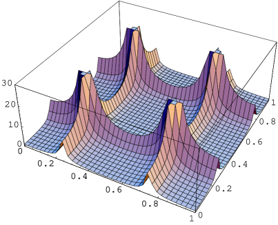
Figure 2: The probability density of the zero mode of quarks in the background of four intersecting planar center vortices [18]. In the two-dimensional cut of the 4-dimensional universe shown in the figure the vortices appear as intersecting lines.

By the Athiya-Singer-Index theorem $\nu=N_{L}-N_{R}$, a non-zero topological charge $\nu$ is connected to the difference between the numbers $N_{L/R}$ of left and right handed quark-zero modes. Figure 2 shows the probabiltiy density of the zero modes of the quarks moving in the backround of two pairs of intersecting center vortices on the 4-dimensional torous [18]. As one observes, the quark-zero modes are concentrated on the center vortex sheets and are in particular localized at the intersection points, the spots of topological charge $\nu=\frac{1}{2}$. If the quark-zero modes dominate the quark propagator the quarks will travel along the center vortex sheets and can move from one vortex to an other through the intersection points. Since the center vortices percolate in the QCD vacuum we expect also the percolation of the quark trajectories, which will eventually result in a condensation of the quarks.

4 Topology of generic center vortices

Generically at a fixed time $t$ a center vortex $\partial\Sigma$ represents a closed magnetic flux loop $C(t)$. For such magnetic flux loops topological charge can be expressed as [10]

$$\nu=\frac{1}{4}\int dt\partial_{t}W\left(C(t)\right),$$ (5)

where $W(C)$ denotes the writhing number of $C$, which is defined as the coincidence limit $W(C)=L(C,C)$ of the Gaussian linking number

$$L\left(C_{1},C_{2}\right) = \frac{1}{4\pi}\oint\limits_{C_{1}}dx_{i}\oint\limits_{C_{2}}dx^{\prime}_{j}\varepsilon_{ijk}\frac{x_{k}-x^{\prime}_{k}}{\left|\vec{x}-\vec{x^{\prime}}\right|^{3}}.$$ (6)

If the writhing number changes continuously during the whole time evolution say from an initial time $t_{i}$ to a final time $t_{f}$ (i.e. $W\left(C(t)\right)$ is a differentiable function of time) the topological charge is given by $\nu=\frac{1}{4}\left(W(t_{f})-W(t_{i})\right)$. However, the writhing number $W(t)$ may change in a discontinuous way, e.g. when two line segments of the vortex loop intersect (see below). If we denote by $\bar{t}_{k},k=1,2,..;t_{i}<\bar{t}_{k}<t_{f}$ the intermediate time instants where $W(t)$ jumps by a finite amount $\Delta W\left(\bar{t}_{k}\right)=\lim\limits_{\varepsilon\rightarrow 0}\left[W\left(\bar{t}_{k}+\varepsilon\right)-W\left(t_{k}-\varepsilon\right)\right]$ the complete expression for the topological charge for a generic center vortex is given by [10]

$$\nu=\frac{1}{4}\left[W\left(t_{f}\right)+\sum\limits_{k}\Delta W\left(\bar{t}_{k}\right)-W\left(t_{i}\right)\right].$$ (7)

This relation will be illustrated below by means of an example.

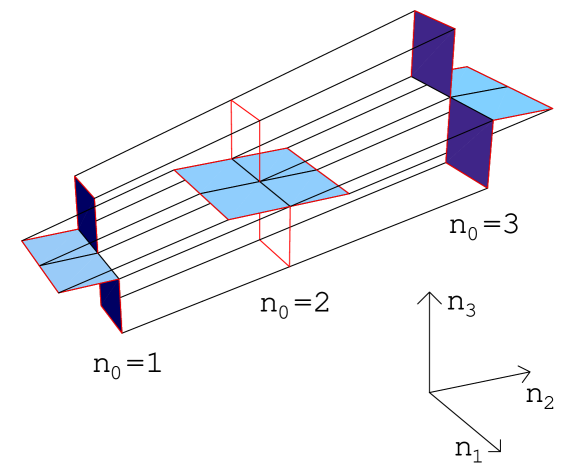
Figure 3: Sample vortex surface configuration taken from [15]. At each lattice time $t=n_{0}a$ (a is the lattice spacing), shaded plaquettes are part of the vortex surface. These plaquettes are furthermore connected to plaquettes running in time direction; their location can be inferred most easily by keeping in mind that each link of the configuration is connected to exactly two plaquettes (i.e. the surface is closed and contains no intersection lines). Note that the two non-shaded plaquettes at $n_{0}=2$ are not part of the vortex; only the two sets of three links bounding them are. These are slices at $n_{0}=2$ of surface segments running in time direction from $n_{0}=1$ through to $n_{0}=3$. Sliced at $n_{0}=2$, these surface segments show up as lines. Furthermore, by successively assigning orientations to all plaquettes, one can convince oneself that the configuration is orientable. The vortex image was generated by means of a MATHEMATICA routine provided by R. Bertle and M. Faber.

5 The writhing number of center vortex loops

To illustrate the various singular vortex points, let us consider as an example the center vortex configuration shown in fig. 3, [15], which could arise in a lattice simulation after center projection [17], or in a random vortex model [14]. This vortex surface is orientable and has various spots of non-zero topological charge: There is a transversal intersection point at the intermediate time $n_{0}=2$ contributing $\frac{1}{2}$ to the topological charge $\nu$. At this time there are also two twisting points at the front and back edges of the configuration, each contributing $-\frac{1}{8}$ to $\nu$. Further twisting points occur at the initial $(n_{0}=1)$ and final $(n_{0}=3)$ times, each contributing $-\frac{1}{8}$ to $\nu$, so that the total topological charge vanishes for this vortex configuration $(\nu=0)$.

Figure 4: Snap shots at characteristic time instants of the continuum center vortex loop whose lattice realization is shown in fig. 3.

Let us now interpret the same configuration as a time dependent vortex loop in ordinary 3-dimensional space (as in a movie-show) eliminating lattice artifacts due to the use of a discretised time [10]. Purely spatial vortex patches can be considered as lattice artifacts. They represent the discrete time step approximation to continuously evolving (in time) vortex loops. Fig. 4 shows the time-evolution of a closed magnetic vortex loop in ordinary 3-dimensional space which on the 4-dimensional lattice gives rise to the configuration shown in fig. 3. For simplicity I have kept the cubistic representation in $D=3$ space, so that the loops consist of straight line segments. At an initial time $t=\bar{t}_{i}$ an infinitesimal closed vortex loop is generated which then growths up to a time $t=\bar{t}_{1}$. Then the long horizontal loop segment moves towards, and at time $t=\bar{t}_{2}$ crosses the long vertical loop segment, and continues to move up to a time $t=\bar{t}_{3}$. After this time the loop decreases continuously and at the fixed time $t=\bar{t}_{f}$ shrinks to a point.

For simplicity let us choose $t_{i}<\bar{t}_{i}$ (the birth of the vortex loop) and $t_{f}>\bar{t}_{f}$ (the death of the vortex loop). Then $W(t_{i})=W(t_{f})=0$ since there are no vortex loops at the initial and final times. In the field configuration shown in fig. 4 there are discontinuous changes of the vortex loop, and accordingly of the writhing number, at the creation (birth) of the vortex loop at $t=\bar{t}_{i}$, at the intermediate time $\bar{t}_{2}$, where two line segments cross and two lines turn by 180 degrees, and at the annihilation (death) of the vortex loop at $t=\bar{t}_{f}$. Hence the topological charge of this configuration is given by (assuming $t_{i}<\bar{t}_{f}$ and $t_{f}>\bar{t}_{f}$)

$$\nu=\frac{1}{4}\left[\Delta W\left(\bar{t}_{f}\right)+\Delta W\left(\bar{t}_{2}\right)+\Delta W\left(\bar{t}_{i}\right)\right]$$ (8)

For simplicity, let us assume that from its creation at $\bar{t}_{i}$ until the time $\bar{t}_{1}$ the vortex loop does not change its shape, but merely scales in size. The same will be assumed for the vortex evolution from $\bar{t}_{3}$ until its annihilation at $\bar{t}_{f}$. Then the change of the writhing number at vortex creation and at annihilation, respectively, is given by $\Delta W(\bar{t}_{i})=W(\bar{t}_{1})$ and $\Delta W(\bar{t}_{f})=-W(\bar{t}_{3})$, so that we obtain for the topological charge (8)

$$\nu=\frac{1}{4}\left[W(\bar{t}_{1})+\Delta W(\bar{t}_{2})-W(\bar{t}_{3})\right].$$ (9)

The writhing numbers $W(\bar{t}_{1}),W(\bar{t}_{3})$ are explicitly evaluated in ref. [10] $W(\bar{t}_{1})=\frac{1}{2},W(\bar{t}_{3})=-\frac{1}{2}$.

A further singular change of the vortex loop shown in fig. 4 occurs at the intermediate time $t=\bar{t}_{2}$. At this time the two long line segments intersect. The crossing of these two line segments at $t=\bar{t}_{2},\left(x,y,z\right)=\left(0,0,0\right)$ corresponds in D=4 to the transversal intersection point shown in fig. 3 at $n_{0}=2$. In fact, in ref. [10] it is shown that the crossing of these two line segments gives rise to a change in the writhing number of $\Delta W\left(\bar{t}_{2}\right)^{(i)}=-2$, which in view of eq. (7) is in accord with the finding [11] that a transversal intersection point contributes $\Delta\nu=\pm\frac{1}{2}$ to the topological charge. Furthermore, when the two long loop segments cross the two short horizontal loop segments at the front and back edges reverse their directions, which can be interpreted as twisting these loop segments by an angle $\pi$ around the $n_{1}$-axis. In the $D=4$ dimensional lattice realization of the present center vortex shown in fig. 3 these twistings of the vortex loop segments (in $D=3$) by angle $\pi$ correspond to the two twisting points at $n_{0}=2$ at the front and back edges of the configuration. As shown in ref. [10] these two twisting points both change the writhing number by $\Delta W\left(\bar{t}_{2}\right)^{t}=\frac{1}{2}$ and hence contribute $\Delta\nu=\frac{1}{8}$ to the topological charge, again in agreement with the analysis of $\nu$ in $D=4$. As a result we find for the total change in the writhing number at $t=\bar{t}_{z},\Delta W\left(\bar{t}_{2}\right)=-2+\frac{1}{2}+\frac{1}{2}=-1$.

In ref. [10] also the twist of the vortex loops was studied. It was found that transversal intersection points, corresponding to the crossing of 2 full line segments, never change the twist, while twisting points, depending on the choosen framing, are usually also connected to changes of the twist, which justifies their name. Finally let us also mention that the description of the topological charge of center vortices in terms of the temporal changes of the writhing number of the time-dependent vortex loops ramains also valid for non-oriented center vortices, i.e. in the presence of magnetic monopole loops.

Acknowledgements:

I thank the organizers, J. Greensite and $\check{S.}$ Olejnik, for bringing us together to this interesting workshop. Discussions with M. Engelhardt, T. Tok and I. Zahed are gratefully acknowledged.

References

-
[1]
G.‘t Hooft, Nucl. Phys. B138 (1978) 1;
Y. Aharonov, A. Casher and S. Yankielowicz, Nucl. Phys. B146 (1978) 256;
J. M. Cornwall, Nucl. Phys. B157 (1979) 392
G. Mack and V. B. Petkova, Ann. Phys. (NY) 123 (1979) 442;
G. Mack, Phys. Rev. Lett. 45 (1980) 1378;
G. Mack and V. B. Petkova, Ann. Phys. (NY) 125 (1989) 117;
G. Mack, in: Recent Developments in Gauge Theories , eds. G. ’t Hooft et al. (Plenum, New York, 1980);
G. Mack and E. Pietarinen, Nucl. Phys. B205 [FS5] (1982) 141
H. B. Nielsen and P. Olesen, Nucl. Phys. B160 (1979) 380;
H. Ambjørn and P. Olesen, Nucl. Phys. B170 [FS1] (1980) 60;
J. J. Ambjørn and P. Olesen, Nucl. Phys. B170 [FS1] (1980) 265;
E. T. Tomboulis, Phys. Rev. D 23 (1981) 2371 - [2] Del Debbio, M. Faber, J. Greensite, . Olejnik, Phys. Rev. D55 (1997) 2298
- [3] K. Langfeld, H. Reinhardt, O. Tennert, Phys. Lett. B419 (1998) 317
- [4] L. Del Debbio. M. Faber, J. Giedt, J. Greensite and . Olejnik, Phys. Rev. D 58 (1998) 094501
- [5] K. Langfeld, O. Tennert, M. Engelhardt and H. Reinhardt, Phys. Lett. B542 (1999) 301, M. Engelhardt, K. Langfeld, H. Reinhardt and O. Tennert, Phys. Rev. D61 (2000) 054504
- [6] T. G. Kovacs, E. T. Tomboulis, Phys. Rev. Lett. 85 (2000) 704
- [7] P. de Forcrand and M. D‘Elia, Phys. Rev. Lett. 82 (1999) 4582.
- [8] M. Nowak, M. Rho, I. Zahed, Chiral Nuclear Dynamics, World Scientific, Singapore, 1996 and references therein
- [9] R. Bertle, M. Engelhardt, M. Faber, Phys. Rev. D64 (2001) 504
- [10] H. Reinhardt, hep-th/0112215, Nucl. Phys. B, in press.
- [11] M. Engelhardt, H. Reinhardt, Nucl. Phys. B567 (2000) 249
- [12] H. Reinhardt, M. Engelhardt, Proceedings of the XVIII Lisbon Autumn School, “Topology of Strongly Correlated Systems”, Lisbon, 8-13 October, 2000, hep-th/0010031
- [13] J. M. Cornwall, Phys. Rev. D61 (2000) 085012
- [14] M. Engelhardt and H. Reinhardt, Nucl. Phys. B585 (2000) 591
- [15] M. Engelhardt, Nucl. Phys. B585 (2000) 614
- [16] H. Reinhardt, Nucl. Phys. B503 (1997) 505
- [17] R. Bertle, M. Faber, J. Greensite. . Olejnik, JHEP 9903 (1999) 019
- [18] H. Reinhardt, O. Schröder, T. Tok, V. Ch. Zhukovsky, hep-th/0203012