Abstract

Using an exact supergravity solution representing the $D_{p}-\bar{D}_{p}$ system, it is demonstrated that one can construct a supergravity analogue of the tachyon potential. Remarkably, the (regularized) minimum value of the potential turns out to be $V(T_{0})=-2m$ with $m$ denoting the ADM mass of a single $D_{p}$-brane. This result, in a sense, appears to confirm that Sen’s conjecture for the tachyon condensation on unstable $D$-branes is indeed correct although the analysis used here is semi-classical in nature and hence should be taken with some care. Also shown is the fact that the tachyon mass squared $m^{2}_{T}$ (which has started out as being negative) can actually become positive definite and large as the tachyon rolls down toward the minimum of its potential. It indeed signals the possibility of successful condensation of the tachyon since it shows that near the minimum of its potential, tachyon can become heavy enough to disappear from the massless spectrum. Some cosmological implications of this tachyon potential in the context of “rolling tachyons” is also discussed.

PACS numbers : 11.25.Sq, 04.65.+e, 11.10.Kk

1 Introduction

Recently, it has been realized that the spectrum in some vacua of type II string theories contains not only BPS $D$-branes but also unstable non-BPS $D$-branes [1, 3]. And the instability of these non-BPS $D$-branes has been interpreted in the stringy context in terms of the tachyonic mode arising in the spectrum of open strings ending on the non-BPS $D$-branes. Indeed, there could be several ways in which one can argue why the tachyonic mode should develop in the spectrum of open strings ending on unstable $D$-branes such as $D_{p}-\bar{D}_{p}$ systems or non-BPS $D_{p}$-branes with “wrong” worldvolume dimensions in IIA/IIB theories. And perhaps one of the simplest albeit formal ways goes as follows in terms of the boundary state formalism [2, 4]. The boundary state describing a $D_{p}$-brane can have a contribution from the closed string $NSNS$ and $RR$ sectors. And on the side of $NSNS$ sector, there is a unique boundary state for each $p$ that implements the correct boundary conditions and survives the corresponding GSO projection. On the side of $RR$ sector, however, there is a unique boundary state only for those $D_{p}$-branes that can couple to a $RR$ tensor potential $A_{[p+1]}$ and for all other values of $p$, the GSO projection kills all possible boundary states in the $RR$ sector. Namely in the boundary state formalism, a supersymmetric $RR$ charged $D_{p}$-brane is represented by

$$|D_{p}>_{BPS}={1\over\sqrt{2}}(|B>_{NSNS}\pm|B>_{RR})$$ (1)

where the sign in front of the $RR$ component of the boundary state determines the $RR$ charge or equivalently the orientation of the brane. On the other hand, for the non-supersymmetric $D_{p}$-brane with wrong values of $p$ in which case $A_{[p+1]}$ is absent and hence carries no $RR$ charge, its boundary state contains only a $NSNS$ component

$$|D_{p}>=|B>_{NSNS}.$$ (2)

Now for this non-supersymmetric $D_{p}$-brane with wrong $p$, the absence of the $RR$ sector in its boundary state implies the absence of the GSO projection in the open string loop channel and as a result, the open string spectrum contains both the lowest-lying tachyonic mode and the next lowest gauge field. Thus to summarize, the spectrum of open strings ending on unstable $D_{p}$-branes is non-supersymmetric and contains a tachyon. For $N$-coincident $D_{p}-\bar{D}_{p}$ pairs, the worldvolume gauge symmetry is $U(N)\times U(N)$ and the tachyon $T$ is in the complex $(N,\bar{N})$ representation whereas for, say, $2N$-coincident unstable $D_{p}$-branes, the worldvolume gauge symmetry is $U(2N)$ and the tachyon is in the adjoint represenration. And in both cases, the tachyon behaves as a Higgs field, rolling down to the minimum of its potential and Higgsing these gauge symmetries. Thus the determination of the associated tachyon potential in these unstable $D_{p}$-brane systems is of primary concern. Moreover, recently the interest in the nature of this tachyon potential has been multipled by the idea of unstable brane decay via the open string tachyon condensation on these unstable $D_{p}$-branes. (For pioneering earlier works on tachyon condensation, see [5].) And central to this is the conjecture by Sen [6] according to which the tachyon potential has a minimum and the negative energy density contribution from the tachyon potential at the minimum should exactly cancel the sum of the tensions of the brane-antibrane pair. Thus the endpoint of the unstable brane-antibrane annihilation should be a closed string vacuum without any $D$-brane.
In the present work, we shall attempt to read off the supergravity analogue of tachyon potential from the semi-classical supergravity description for brane-antibrane interaction. To this end, we begin with the brief review of Sen’s conjecture for tachyon condensation in the brane-antibrane annihilation process which can be stated as follows. It has been known for sometime that a complex tachyon field $T$ with mass squared $m^{2}_{T}=-1/\alpha^{\prime}$ lives in the worldvolume of a coincident $D_{2p}-\bar{D}_{2p}$ pair in type IIA string theory. The tachyon potential should be obtained by integrating out all other massive modes in the spectrum of open strings on the worldvolume and it gets its maximum at $T=0$. Since there is a $U(1)\times U(1)$ Born-Infeld gauge theory living in the worldvolume of this brane-antibrane system, the tachyon field $T$ picks up a phase under each of these $U(1)$ gauge transformations. As a result, the tachyon potential $V(T)$ is a function only of $|T|$ and its minimum occurs at $T=T_{0}e^{i\theta}$ for some arbitrary, but fixed value $T_{0}$. Now Sen goes on to argue that at $T=T_{0}$, the sum of the tension of $D$-brane and anti-$D$-brane and the minimum negative potential energy of the tachyon is exactly zero

$$V(T_{0})+2M_{D}=0$$

with $M_{D}=T_{D}$ being the $D$-brane tension. And the philosophy underlying this conjecture is the physical expectation that the endpoint of the brane-antibrane annihilation would be a closed string vacuum in which the supersymmetry is fully restored. Unfortunately, however, the tachyon potential here $V(T)$ is not something that can be calculated at the moment in a rigorous way although there has been numerous attempts and considerable achievements, say, in the context of open string field theory [7]. In the present work, using a known, exact supergravity solution representing a $D_{p}-\bar{D}_{p}$ system (particularly for $p=6$), we shall demonstrate in a rigorous manner that one can construct a “supergravity analogue” of the tachyon potential and it may possesses essential nature which could be typical in the genuine, stringy tachyon potential. Some recent works discussing interesting related issues on the decay of brane-antibrane systems also appeared in the literature [8, 9].

2 Exact supergravity solution for a brane-antibrane pair

In this section, we shall discuss the exact supergravity solutions representing the $D6/anti-D6$ ($D6-\bar{D6}$ heceforth) system and the intersection of this $D6/anti-D6$ with a magnetic $RR$ flux 7-brane ($(D6-\bar{D6})||F7$ for short, henceforth). The former possesses conical singularities which can be made to disappear by introducing the $RR$ magnetic field (i.e., the $RR$ $F7$-brane) and properly tuning its strength in the latter. In order to demonstrate this, we need to along the way perform the M-theory uplift of the $D6-\bar{D6}$ pair which leads to the Kaluza-Klein ($KK$) monopole/anti-monopole solution ($KK-dipole$ henceforth) first discussed in the literature by Sen [10] by embedding the Gross-Perry [11] $KK-dipole$ solution in $D=11$ M-theory context. Indeed the $D6$-brane solution is unique among $D_{p}$-brane solutions in IIA/IIB theories in that it is a codimension 3 object and hence in many respects behaves like the familiar abelian magnetic monopole in $D=4$. This, in turn, implies that the $D6-\bar{D6}$ solution should exhibit essentially the same generic features as those of Bonnor’s magnetic dipole solution [12, 13] and its dilatonic generalizations [14, 13] in $D=4$ studied extensively in the recent literature. As we shall see in a moment, these similarities allow us to envisage the generic nature of instabilities common in all unstable $D_{p}-\bar{D}_{p}$ systems in a simple and familiar manner.

2.1 $D6-\bar{D6}$ pair in the absence of the magnetic field

In string frame, the exact IIA supergravity solution representing the $D6-\bar{D6}$ pair is given by [15, 13]

$$ds^{2}_{10} = H^{-1/2}[-dt^{2}+\sum^{6}_{i=1}dx^{2}_{i}]+H^{1/2}[(\Delta+a^{2}\sin^{2}\theta)\left({dr^{2}\over\Delta}+d\theta^{2}\right)+\Delta\sin^{2}\theta d\phi^{2}],$$

$$e^{2\phi} = H^{-3/2},$$ (3)

$$A_{[1]} = \left[{2mra\sin^{2}\theta\over{\Delta+a^{2}\sin^{2}\theta}}\right]d\phi,~{}~{}~{}F_{[2]}=dA_{[1]}$$

where the “modified” harmonic function in 3-dimensional transverse space is given by

$$H(r)={\Sigma\over{\Delta+a^{2}\sin^{2}\theta}}$$ (4)

and $\Sigma=r^{2}-a^{2}\cos^{2}\theta$, $\Delta=r^{2}-2mr-a^{2}$ with $r$ being the radial coordinate in the transverse directions. The parameter $a$ can be thought of as representing the separation between the brane and antibrane (we will elaborate on this shortly) and changing the sign of $a$ amounts to reversing the orientation of the brane pair, so here we will choose, without loss of generality, $a\geq 0$. $m$ is the ADM mass of each brane and the ADM mass of the whole $D6-\bar{D6}$ system is $M_{ADM}=2m$ which should be obvious as it would be the sum of ADM mass of each brane when they are well separated. It is also noteworthy that, similarly to what happens in the Ernst solution [16] in $D=4$ Einstein-Maxwell theory describing a pair of oppositely-charged black holes accelerating away from each other (due to the Melvin magnetic universe content), this $D6-\bar{D6}$ solution in IIA theory is also static but axisymmetric in these Boyer-Lindquist-type coordinates. As has been pointed out by Sen [10] in the M-theory $KK-dipole$ solution case and by Emparan [13] in the case of generalized Bonnor’s solution, the IIA theory $D6-\bar{D6}$ solution given above represents the configuration in which a $D6$-brane and a $\bar{D6}$-brane are sitting on the endpoints of the dipole, i.e., $(r=r_{+},\theta=0)$ and $(r=r_{+},\theta=\pi)$ respectively where $r_{+}$ is the larger root of $\Delta=0$, namely $r_{+}=m+\sqrt{m^{2}+a^{2}}$. We now elaborate on our earlier comment that the parameter $a$ appearing in this supergravity solution can be regarded as indicating the proper separation between the brane and the antibrane. Notice first that for large $a$, the proper inter-brane distance increases as $\sim 2a$. Namely,

$$l = \int^{\pi}_{0}d\theta\sqrt{g_{\theta\theta}}|_{r=r_{+}}=\int^{\pi}_{0}d\theta H^{1/4}(\Delta+a^{2}\sin^{2}\theta)^{1/2}|_{r=r_{+}}$$ (5)

$$\simeq \int^{\pi}_{0}d\theta a\sin\theta=2a.$$

Meanwhile, as argued by Sen [10], the proper inter-brane distance vanishes when $a\rightarrow 0$. In addition, that the limit $a\rightarrow 0$ actually amounts to the vanishing inter-brane distance can be made more transparent as follows. Recently, Brax, Mandal and Oz [17] discussed the supergravity solution representing coincident $D_{p}-\bar{D}_{p}$ pairs in type II theories and studied its instability in terms of the condensation of tachyon arising in the spectrum of open strings stretched between $D_{p}$ and $\bar{D}_{p}$. Thus now, taking the $p=6$ case for example, we first would like to establish the correspondence between our solution given above representing $D6-\bar{D6}$ pair generally separated by an arbitrary distance and theirs. For specific but appropriate values of the parameters appearing in their solution, $(c_{2}=1(p>3),c_{1}=0,r_{0}=m/2)$ [17] so as to represent a neutral, coincident $D6-\bar{D6}$ pair, their solution is given in Einstein frame by

$$ds^{2}_{E} = \left[{1-r_{0}/\tilde{r}\over 1+r_{0}/\tilde{r}}\right]^{1/4}[-dt^{2}+\sum^{6}_{i=1}dx^{2}_{i}]+\left[1-{r_{0}\over\tilde{r}}\right]^{1/4}\left[1+{r_{0}\over\tilde{r}}\right]^{15/4}[d\tilde{r}^{2}+\tilde{r}^{2}(d\theta^{2}+\sin^{2}\theta d\phi^{2})],$$

$$e^{\phi} = \left[{1-r_{0}/\tilde{r}\over 1+r_{0}/\tilde{r}}\right]^{3/2},~{}~{}~{}A_{[1]}=0$$ (6)

which, in string frame, using $g^{E}_{\mu\nu}=e^{-\phi/2}g^{S}_{\mu\nu}$, becomes

$$ds^{2} = \left[{1-r_{0}/\tilde{r}\over 1+r_{0}/\tilde{r}}\right][-dt^{2}+\sum^{6}_{i=1}dx^{2}_{i}]+\left[1-{r_{0}\over\tilde{r}}\right]\left[1+{r_{0}\over\tilde{r}}\right]^{3}[d\tilde{r}^{2}+\tilde{r}^{2}(d\theta^{2}+\sin^{2}\theta d\phi^{2})],$$

$$e^{\phi} = \left[{1-r_{0}/\tilde{r}\over 1+r_{0}/\tilde{r}}\right]^{3/2},~{}~{}~{}A_{[1]}=0.$$ (7)

Consider now, transforming from this isotropic coordinate $\tilde{r}$ to the standard radial $r$ coordinate

$$\tilde{r}={1\over 2}[(r-2r_{0})+(r^{2}-4r_{0}r)^{1/2}]~{}~{}~{}{\rm or~{}inversely}~{}~{}~{}r=\tilde{r}\left(1+{r_{0}\over\tilde{r}}\right)^{2}.$$ (8)

Then their solution describing $(N=1)D6$ and $(\bar{N}=1)\bar{D6}$ now takes the form

$$ds^{2} = \left(1-{2m\over r}\right)^{1/2}[-dt^{2}+\sum^{6}_{i=1}dx^{2}_{i}]+\left(1-{2m\over r}\right)^{-1/2}[dr^{2}+r^{2}\left(1-{2m\over r}\right)(d\theta^{2}+\sin^{2}\theta d\phi^{2})],$$

$$e^{2\phi} = \left(1-{2m\over r}\right)^{3/2},~{}~{}~{}A_{[1]}=0.$$ (9)

Clearly, this solution indeed coincides with the $a\rightarrow 0$ (i.e., vanishing separation) limit of our more general $D6-\bar{D6}$ solution given in eq.(4). Actually, this aspect also has been pointed out in a recent literature [18]. And this confirms our earlier proposition that $a$ indeed acts as a relevant parameter representing the proper inter-brane distance even for very small separation.
Next, we turn to the conical singularity structure of this $D6-\bar{D6}$ solution. First observe that the rotational Killing field $\psi^{\mu}=(\partial/\partial\phi)^{\mu}$ possesses vanishing norm, i.e., $\psi^{\mu}\psi_{\mu}=g_{\alpha\beta}\psi^{\alpha}\psi^{\beta}=g_{\phi\phi}=0$ at the locus of $r=r_{+}$ as well as along the semi-infinite lines $\theta=0,\pi$. This implies that $r=r_{+}$ can be thought of as a part of the symmetry axis of the solution. Namely unlike the other familiar axisymmetric solutions, for the case of the $D6-\bar{D6}$ solution under consideration, the endpoints of the two semi-axes $\theta=0$ and $\theta=\pi$ do not come to join at a common point. Instead, the axis of symmetry is completed by the segment $r=r_{+}$. And as $\theta$ varies from $0$ to $\pi$, one moves along the segment from $(r=r_{+},\theta=0)$ where $D6$ is situated to $(r=r_{+},\theta=\pi)$ where $\bar{D6}$ is placed. Then the natural question to be addressed is whether or not the conical singularities arise on different portions of the symmetry axis. This situation is very reminiscent of the conical singularity structure in the generalized Bonnor’s dipole solution in Einstein-Maxwell-dilaton theory in $D=4$ extensively studied by Emparan [13] recently. Thus below, we explore the nature of possible conical singularities in this $D6-\bar{D6}$ solution in $D=10$ type IIA theory following essentially the same avenue as that presented in the work of Emparan [13]. Namely, consider that ; if $C$ is the proper length of the circumference around the symmetry axis and $R$ is its proper radius, then the occurrence of a conical angle deficit (or excess) $\delta$ would manifest itself if $(dC/dR)|_{R\rightarrow 0}=2\pi-\delta$. We now proceed to evaluate this conical deficit (or excess) assuming first that the azimuthal angle coordinate $\phi$ is identified with period $\Delta\phi$. The conical deficit along the axes $\theta=0,\pi$ and along the segment $r=r_{+}$ are given respectively by

$$\delta_{(0,\pi)} = 2\pi-\arrowvert{\Delta\phi d\sqrt{g_{\phi\phi}}\over\sqrt{g_{\theta\theta}}d\theta}\arrowvert_{\theta=0,\pi}=2\pi-\Delta\phi,$$ (10)

$$\delta_{(r=r_{+})} = 2\pi-\arrowvert{\Delta\phi d\sqrt{g_{\phi\phi}}\over\sqrt{g_{rr}}dr}\arrowvert_{r=r_{+}}=2\pi-\left(1+{m^{2}\over a^{2}}\right)^{1/2}\Delta\phi$$

where, of course, we used the $D6-\bar{D6}$ metric solution given in eq.(4). From eq.(11), it is now evident that one cannot eliminate the conical singularities along the semi-axes $\theta=0,\pi$ and along the segment $r=r_{+}$ at the same time. Indeed one has the options :
(i) One can remove the conical angle deficit along $\theta=0,\pi$ by choosing $\Delta\phi=2\pi$ at the expense of the conical angle excess along $r=r_{+}$ which amounts to the presence of a strut providing the internal pressure to counterbalance the combined gravitational and gauge attractions between $D6$ and $\bar{D6}$.
(ii) Alternatively, one can instead eliminate the conical singulatity along $r=r_{+}$ by choosing $\Delta\phi=2\pi(1+m^{2}/a^{2})^{-1/2}$ at the expense of the appearance of the conical angle deficit $\delta_{(0,\pi)}=2\pi[1-\{a^{2}/(m^{2}+a^{2})\}^{1/2}]$ along $\theta=0,\pi$ which implies the presence of cosmic strings providing the tension

$$\tau={\delta_{(0,\pi)}\over 8\pi}={1\over 4}\left[1-\left({a^{2}\over m^{2}+a^{2}}\right)^{1/2}\right]$$

that pulls $D6$ and $\bar{D6}$ at the endpoints apart.
Normally, one might wish to take the second option in which the pair of branes is suspended by open cosmic strings, namely $D6$ and $\bar{D6}$ are kept apart by the tensions generated by cosmic strings against the collapse due to the gravitational and gauge attractions. And the line $r=r_{+}$, $0<\theta<\pi$ joining $D6$ and $\bar{D6}$ is now completely non-singular. This recourse to cosmic strings to account for the conical singularities of the solution and to suspend the $D6-\bar{D6}$ system in an equilibrium configuration, however, might appear as a rather ad hoc prescription. Perhaps it would be more relevant to introduce an external magnetic field aligned with the axis joining the brane pair to counterbalance the combined gravitational and gauge attractions by pulling them apart. By properly tuning the strength of the magnetic field, the attractive inter-brane force along the axis would be rendered to vanish. Indeed this conical singularity structure of the $D6-\bar{D6}$ system and its cure via the introduction of the external magnetic field of proper strength is reminiscent of Ernst’s prescription [16] for the elimination of conical singularities of the charged $C$-metric and of Emparan’s treatment [13] to remove the analogous conical singularities of the Bonnor’s magnetic dipole solution in Einstein-Maxwell and Einstein-Maxwell-dilaton theories and in the present work, we are closely following the formulation of Emparan [13].

2.2 $D6-\bar{D6}$ pair in the presence of the magnetic field

In order to introduce the external magnetic field with proper strength to counterbalance the combined gravitational and gauge attractions and hence to keep the $D6-\bar{D6}$ pair in an (unstable) equilibrium configuration, we now proceed to construct the supergravity solution representing $D6-\bar{D6}$ pair parallely intersecting with a $RR$ $F7$-brane. This can be achieved by first uplifting the $D6-\bar{D6}$ solution in IIA theory to the $D=11$ $KK-dipole$ solution in M-theory discussed by Sen [10] and then by performing a twisted KK-reduction on this M-theory $KK-dipole$. Thus consider carrying out the dimensional lift of the $D6-\bar{D6}$ solution given in eq.(4) to $D=11$ via the standard KK-ansatz

$$ds^{2}_{11}=e^{-{2\over 3}\phi}ds^{2}_{10}+e^{{4\over 3}\phi}(dy+A_{\mu}dx^{\mu})^{2}$$ (11)

(with $A_{[1]}=A_{\mu}d^{\mu}$ being the 1-form magnetic $RR$ potential in eq.(4)) which yields

$$ds^{2}_{11} = [-dt^{2}+\sum^{6}_{i=1}dx^{2}_{i}]+\Sigma\left[{dr^{2}\over\Delta}+d\theta^{2}\right]$$

$$+ {1\over\Sigma}[\Delta(dy-a\sin^{2}\theta d\phi)^{2}+\sin^{2}\theta\{(r^{2}-a^{2})d\phi+ady\}^{2}].$$

This is the $KK$ monopole/anti-monopole solution in $D=11$ or the M-theory $KK-dipole$ solution first given by Sen [10]. Similarly to the IIA theory $D6-\bar{D6}$ solution discussed above, this M-theory $KK-dipole$ solution represents the configuration in which $KK$ monopole and anti-monopole are sitting on the endpoints of the dipole, i.e., $(r=r_{+},\theta=0)$ and $(r=r_{+},\theta=\pi)$ respectively. Note that unlike the IIA theory $D6-\bar{D6}$ solution, this M-theory $KK-dipole$ solution is free of conical singularities provided the azimuthal angle coordinate $\phi$ is periodically identified with the standard period of $2\pi$. Now to get back down to $D=10$, consider performing the non-trivial point identification

$$(y,~{}\phi)\equiv(y+2\pi n_{1}R,~{}\phi+2\pi n_{1}RB+2\pi n_{2})$$ (13)

(with $n_{1},~{}n_{2}\in Z$) on the M-theory $KK-dipole$ solution in eq.(14), followed by the associated skew KK-reduction along the orbit of the Killing field

$$l=\left(\partial/\partial y\right)+B\left(\partial/\partial\phi\right)$$ (14)

where $B$ is a magnetic field parameter. And this amounts to introducing the adapted coordinate

$$\tilde{\phi}=\phi-By$$ (15)

which is constant along the orbits of $l$ and possesses standard period of $2\pi$ and then proceeding with the standard KK-reduction along the orbit of $(\partial/\partial y)$. Thus we recast the metric solution, upon changing to this adapted coordinate, in the standard KK-ansatz

$$ds^{2}_{11} = [-dt^{2}+\sum^{6}_{i=1}dx^{2}_{i}]+\Sigma\left[{dr^{2}\over\Delta}+d\theta^{2}\right]+{\Delta+a^{2}\sin^{2}\theta\over\Sigma}dy^{2}$$ (16)

$$+ {2[(r^{2}-a^{2})-\Delta]a\sin^{2}\theta\over\Sigma}dy(d\tilde{\phi}+Bdy)+{\sin^{2}\theta\over\Sigma}[(r^{2}-a^{2})^{2}+\Delta a^{2}\sin^{2}\theta](d\tilde{\phi}+Bdy)^{2}$$

$$= e^{-{2\over 3}\phi}ds^{2}_{10}+e^{{4\over 3}\phi}(dy+A_{\mu}dx^{\mu})^{2}$$

and then read off the $10$-dimensional fields as

$$ds^{2}_{10} = \Lambda^{1/2}\left\{[-dt^{2}+\sum^{6}_{i=1}dx^{2}_{i}]+\Sigma\left[{dr^{2}\over\Delta}+d\theta^{2}\right]\right\}+\Lambda^{-1/2}\Delta\sin^{2}\theta d\tilde{\phi}^{2},$$

$$e^{{4\over 3}\phi} = \Lambda,$$ (17)

$$A_{[1]} = \Lambda^{-1}{\sin^{2}\theta\over\Sigma}\left\{B[(r^{2}-a^{2})^{2}+\Delta a^{2}\sin^{2}\theta]+a[(r^{2}-a^{2})-\Delta]\right\}d\tilde{\phi},$$

$$F_{[2]} = (\partial_{r}A_{\tilde{\phi}})dr\wedge d\tilde{\phi}+(\partial_{\theta}A_{\tilde{\phi}})d\theta\wedge d\tilde{\phi},~{}~{}~{}{\rm where}$$

$$\Lambda = {1\over\Sigma}\left\{[\Delta+a^{2}\sin^{2}\theta]+2Ba\sin^{2}\theta[(r^{2}-a^{2})-\Delta]+B^{2}\sin^{2}\theta[(r^{2}-a^{2})^{2}+\Delta a^{2}\sin^{2}\theta]\right\}.$$

Note that this solution can be identified with a $D6-\bar{D6}$ pair parallely intersecting with a magnetic $RR$ $F7$-brane since for $B=0$, it reduces to the $D6-\bar{D6}$ solution in eq.(4) while for $m=0$ and $a=0$, it reduces to a $RR$ $F7$-brane solution in IIA theory. To see this last point explicitly, we set $m=0=a$ in eq.(19) to get

$$ds^{2}_{10} = \Lambda^{1/2}\left[-dt^{2}+\sum^{6}_{i=1}dx^{2}_{i}+dr^{2}+r^{2}d\theta^{2}\right]+\Lambda^{-1/2}r^{2}\sin^{2}\theta^{2}d\tilde{\phi}^{2},$$

$$e^{2\phi} = \Lambda^{3/2},$$ (18)

$$A_{[1]} = A_{\tilde{\phi}}d\tilde{\phi}={Br^{2}\sin^{2}\theta\over(1+B^{2}r^{2}\sin^{2}\theta)}~{}~{}~{}{\rm where~{}~{}now}$$

$$\Lambda = (1+B^{2}r^{2}\sin^{2}\theta).$$

Clearly, this is a magnetic $RR$ $F7$-brane solution in type IIA theory. Also note that generally a $D_{2p}$-brane has a direct coupling to a $RR$ $F_{(2p+1)}$-brane in IIA theory. Thus for the case at hand, the magnetic $D6$ and $\bar{D6}$-brane content of the solution in eq.(19) couple directly to the magnetic $RR$ 1-form potential of the $F7$-brane content extracted in eq.(20) and as a result experience static Coulomb-type force that eventually keeps the $D6-\bar{D6}$ pair apart against the gravitational and gauge attractions.
Lastly, we see if the conical singularities which were inevitably present in the $D6-\bar{D6}$ seed solution can now be eliminated by the introduction of this magnetic $F7$-brane content. To do so, notice that in this $(D6-\bar{D6})||F7$ case, $\psi^{\mu}\psi_{\mu}=g_{\tilde{\phi}\tilde{\phi}}=0$ has roots at the locus of $r=r_{+}$ as well as along the semi-infinite axes $\theta=0,\pi$. Thus we need to worry about the possible occurrence of conical singularities both along $\theta=0,\pi$ and at $r=r_{+}$ again. Assuming that the azimuthal angle coordinate $\tilde{\phi}$ is identified with period $\Delta\tilde{\phi}$, the conical deficit along the axes $\theta=0,\pi$ and along the segment $r=r_{+}$ are given respectively by

$$\delta_{(0,\pi)} = 2\pi-\arrowvert{\Delta\tilde{\phi}d\sqrt{g_{\tilde{\phi}\tilde{\phi}}}\over\sqrt{g_{\theta\theta}}d\theta}\arrowvert_{\theta=0,\pi}=2\pi-\Delta\tilde{\phi},$$ (19)

$$\delta_{(r=r_{+})} = 2\pi-\arrowvert{\Delta\tilde{\phi}d\sqrt{g_{\tilde{\phi}\tilde{\phi}}}\over\sqrt{g_{rr}}dr}\arrowvert_{r=r_{+}}=2\pi-\left[{r_{+}-m\over B(r^{2}_{+}-a^{2})+a}\right]\Delta\tilde{\phi}$$

where, in this time, we used the $(D6-\bar{D6})||F7$ metric solution given in eq.(19). Therefore, by choosing $\Delta\tilde{\phi}=2\pi$ and “tuning” the strength of the external magnetic field as

$$B={(r_{+}-m)-a\over(r^{2}_{+}-a^{2})}={\sqrt{m^{2}+a^{2}}-a\over 2mr_{+}}$$ (20)

one now can remove all the conical singularities. As stated earlier, this removal of conical singularities by properly tuning the strength of the magnetic field amounts to suspending the $D6-\bar{D6}$ pair in an (unstable) equilibrium configuration by introducing a force exerted by this magnetic field (i.e., the $RR$ $F7$-brane) to counterbalance the combined gravitational and gauge attractive force. To see this in a qualitative manner [10], recall first that, when they are well separated, the distance between $D6$ and $\bar{D6}$ is given roughly by $\sim 2a$ as shown in eq.(6) and in this large-$a$ limit, the magnetic field strength given above in eq.(22) is $B\simeq m/4a^{2}$. Next, since both the gravitational and $RR$ gauge attractive forces between the branes would be given by $m^{2}/(2a)^{2}$ (where we used the fact that the $RR$-charge of a $D6$-brane behaves like $q\rightarrow m$ for large inter-brane separation as discussed earlier), the total attractive force goes like $m^{2}/2a^{2}$. Thus this combined attractive force would be counterbalanced by the repulsive force on the magetic dipole of the $D6-\bar{D6}$ pair, $2qB\simeq 2m(m/4a^{2})=m^{2}/2a^{2}$ provided by the properly tuned magnetic field strength $B$ of $RR$ $F7$-brane give above in eq.(22).

3 Supergravity analogue of tachyon potential

Since our strategy is to attempt to read off the supergravity analogue of tachyon potential from the semi-classical supergravity description for the brane-antibrane interaction, we now start with the evaluation of the interaction energy between the brane and antibrane and in this work, we particularly take the case of $D6$-brane. Before we proceed, however, a cautious comment might be relevant. That is, throughout we shall take the parameter $a$ appearing in the supergravity solution for $D6-\bar{D6}$ system as representing the proper distance between the brane and the antibrane. Thus one might question if this parameter $a$ can really serve to represent the inter-brane separation all the way from large-$a$ to $a\rightarrow 0$, i.e., even to the case of nearly coincident $D6-\bar{D6}$ system when the tachyonic mode is supposed to develop in the spectrum of open strings stretched between $D6$ and $\bar{D6}$. First, recall that we already demonstrated that for large separation, the proper inter-brane distance grows as $l\simeq 2a$ confirming the role of the parameter $a$ just argued. Also recall that earlier, we exhibited the fact that our supergravity solution for the $D6-\bar{D6}$ pair does indeed reduce, in the limit, $a\rightarrow 0$, to the solution for the coincident $D6-\bar{D6}$ pair known in the literature [17]. And this last point indicates that evidently, $a$ still acts as a relevant parameter representing the proper inter-brane distance even for very small separation. Thus to conclude, we may employ $a$ as a relevant parameter in the supergravity solution representing the inter-brane distance all the way. Now, coming back to our main interest, notice first that in the absence of the magnetic field (i.e., the magnetic $RR$ $F7$ brane), the total energy (i.e., the ADM-mass of the system) of the asymptotically-flat $D6-\bar{D6}$ solution given earlier is $2m$. This is because in the limit of infinite separation $a\rightarrow\infty$, the interaction energy between the branes should vanish and thus the total energy should be twice the ADM-mass of a single brane, $m$. In the presence of the magnetic field, however, the supergravity solution is no longer asymptotically-flat, but instead is asymptotic to the Melvin-type universe. Nevertheless, following the treatment suggested by Hawking and Horowitz [19], it is still possible to compute the total energy of the system by taking the generalized Melvin universe as the reference background and hence subtracting out its infinite energy. And the result is that the regularized total energy is still equal to $2m$. Now for finite separation, one would expect non-vanishing interaction energy and it would be given by

$$E_{int}=E_{tot}-2M_{D6}=2m-2Q$$ (21)

where we used the fact that for an extremal (black) brane in isolation, $M_{D_{p}}=Q$. Thus now what remains to be done is to compute the magnetic $RR$ charge $Q$ of the $D6$-brane, in the presence/absence of the content of $RR$ $F7$-brane.

3.1 In the absence of the magnetic field

In order to compute the $RR$ charge of a single $D6$-brane, we certainly need the behavior of the supergravity solution for $D6-\bar{D6}$ pair in the region very close to each of the branes since the charge is given by the integral $Q=(1/4\pi)\int_{S^{2}}F^{n}_{[2]}$, which is over a Gaussian surface having the topology of $S^{2}$ and enclosing each brane. Indeed, it is possible to demonstrate explicitly that in the $D6-\bar{D6}$ solution given earlier in eq.(4), the metric near $(r=r_{+},\theta=0)$ represents that of (distorted) $D6$-brane while the metric near $(r=r_{+},\theta=\pi)$ does that of (distorted) $\bar{D6}$-brane. Thus in order to study the behavior of the $D6-\bar{D6}$ solution in the region very close to the $D6$-brane, we perform the change of coordinates from $(r,\theta)$ to $(\rho,\bar{\theta})$ given by the transformation law [10, 13]

$$r=r_{+}+{\rho\over 2}(1+\cos\bar{\theta}),~{}~{}~{}\sin^{2}\theta={\rho\over\sqrt{m^{2}+a^{2}}}(1-\cos\bar{\theta})$$ (22)

where $r_{+}=m+\sqrt{m^{2}+a^{2}}$ as given earlier. Then taking $\rho$ to be much smaller than any other length scale involved so as to get near each pole, the $D6-\bar{D6}$ solution in eq.(4) becomes

$$ds^{2}_{10} \simeq g^{1/2}(\bar{\theta})\left({\rho\over q}\right)^{1/2}[-dt^{2}+\sum^{6}_{i=1}dx^{2}_{i}]+\left({q\over\rho}\right)^{1/2}[g^{1/2}(\bar{\theta})(d\rho^{2}+\rho^{2}d\bar{\theta}^{2})+g^{-1/2}(\bar{\theta})\rho^{2}\sin^{2}\bar{\theta}d\phi^{2}],$$

$$e^{2\phi} \simeq \left({\rho\over q}\right)^{3/2}g^{3/2}(\bar{\theta}),$$ (23)

$$A^{m}_{[1]} \simeq {mr_{+}a\over(m^{2}+a^{2})}g^{-1}(\bar{\theta})(1-\cos\bar{\theta})d\phi$$

where $q=mr_{+}/\sqrt{m^{2}+a^{2}}$ and $g(\bar{\theta})=cos^{2}(\bar{\theta}/2)+[a^{2}/(m^{2}+a^{2})]\sin^{2}(\bar{\theta}/2)$. Namely in this small-$\rho$ limit, the geometry of the solution reduces to that of the near-horizon limit of a $D6$-brane. However, the horizon is no longer spherically-symmetric and is deformed due to the presence of the other brane, i.e., the $\bar{D6}$-brane located at the other pole. To elaborate on this point, it is noteworthy that the surface $r=r_{+}$ is still a horizon, but instead of being spherically-symmetric, it is elongated along the axis joining the poles in a prolate shape. Namely, the horizon turns out to be a prolate spheroid with the distortion factor given by $g(\bar{\theta})$. And of course, it is further distorted by a conical defect at the poles. And similar analysis can be carried out near the other pole at which $\bar{D6}$ is situated.
We are now ready to compute the $RR$ charge of a single $D6$-brane. Using the Gauss’ law, the $RR$ charge is given by

$$Q = {1\over 4\pi}\int_{S^{2}}F^{m}_{[2]}={1\over 4\pi}\int_{\partial S^{2}}A^{m}_{[1]}$$

$$= {1\over 4\pi}\left[\int^{\Delta\phi}_{0}A_{\phi}d\phi|_{\bar{\theta}=\pi}-\int^{\Delta\phi}_{0}A_{\phi}d\phi|_{\bar{\theta}=0}\right]$$

$$= {\Delta\phi\over 4\pi}[A_{\phi}(\bar{\theta}=\pi)-A_{\phi}(\bar{\theta}=0)]={\Delta\phi\over 2\pi}{mr_{+}\over a}$$

where we used the fact that the boundary of $S^{2}$ enclosing each $D6$-brane consists of two $S^{1}$s with period $\Delta\phi$, one encircling the segment $r=r_{+}$ corresponding to $\bar{\theta}=\pi$ and the other encircling the semi-infinite line $\theta=0$ (or $\pi$) corresponding to $\bar{\theta}=0$. Particularly, if we take $\Delta\phi=2\pi$ to remove deficit angles along $\theta=0,\pi$, the magnetic $RR$ charge turns out to be

$$Q={mr_{+}\over a}=m\left[{m+\sqrt{m^{2}+a^{2}}}\over a\right]$$ (25)

and hence the interaction energy is given by

$$E_{int}=2m-2Q=-2m\left[{{m+\sqrt{m^{2}+a^{2}}}\over a}-1\right]$$ (26)

which obviously is negative, reflecting the fact that the net force between $D6$ and $\bar{D6}$ is attractive as expected. Having obtained the interaction energy of the $D6-\bar{D6}$ system, we now construct the supergravity analogue of the tachyon potential out of it. As was mentioned earlier in the introduction, Sen [6] conjectured that at the minimum (i.e., the true vacuum) of the tachyon potential characterized by the true vacuum expectation value (vev) of the tachyon field $T=T_{0}$, the total energy of a $D_{p}-\bar{D}_{p}$ system should vanish ;

$$E_{tot}=V(T_{0})+2M_{D_{p}}=0$$ (27)

where $M_{D_{p}}$ denotes the mass of a $D_{p}$-brane. Since we look for an analogue of the tachyon potential in the supegravity description, we first try to identify the supergravity counterpart of the equation, leading to the above conjecture, with

$$M_{ADM}=V(T)+2M_{D_{p}}$$ (28)

where now $M_{ADM}$ and $M_{D_{p}}$ stand for the ADM mass of the whole system and that of a single brane respectively. Then it seems natural to assume that the interaction energy between the brane and antibrane for small but finite separation, as the one we just discussed above, should be identified with $V(T)$ since for an isolated extremal $D_{p}$-brane, $M_{D_{p}}=Q$, namely, $V(T)=M_{ADM}-2M_{D_{p}}=E_{tot}-2Q=E_{int}.$ Indeed, this identification may be justified by the fact that the semi-classical instability in the brane-antibrane system, reflected in eq.(28) which indicates the negative interaction energy and hence the attractive force between the branes, should be taken over, as the inter-brane distance gets smaller, by the stringy one in terms of the tachyon condensation. Thus the semi-classical interaction energy for larger inter-brane distance and the tachyon potential for smaller separation should eventually be interpolated properly. Next, since we set $V(T)=E_{int}$, we now need to relate the parameter $a$ in the supergravity solution representing the inter-brane separation to the tachyon field expectation value $|T|$. Indeed, this proper inter-brane distance parameter $a$ in our supergravity analysis is the only parameter that can be probed and related to $|T|$. To this end, we note that :
(i) Since the tachyon field living in the worldvolume of a $D_{p}-\bar{D}_{p}$ system is complex, its potential $V(T)$ is a function only of $|T|^{2}$ [6]. As a consequence, we expect that $a$ should be a function of $|T|^{2}$ as well, and
(ii) the tachyon potential vanishes only at $T=0$ and gets its minimum at $|T|=|T_{0}|$ [6].
Therefore, these observations lead us to suggest that

$$|T|^{2}=|T_{0}|^{2}e^{-a^{2}/l^{2}_{s}},~{}~{}~{}{\rm or}~{}~{}~{}a^{2}=l^{2}_{s}\ln{{|T_{0}|^{2}\over|T|^{2}}}$$ (29)

where the string length $l^{2}_{s}=\alpha^{\prime}$ has been inserted for dimensional consideration since the exponent has to be dimensionless (note that the parameter $a$ and $m$ carry the dimensions of the length). Our proposal, the eq.(31), to relate the proper inter-brane distance $a$ to the tachyon field expectation value $|T|$ and hence to convert the semi-classical interaction energy into the tachyon potential, of course, shows its inevitable limitations as a supergravity approach. Firstly, it can only accomodate the facts that for the inter-brane separation of order $a\sim l_{s}$, the tachyon just develops and is sitting on the false vacuum located at $|T|\simeq 0$ and then “rolls down” toward the true vacuum (minimum of its potential) located at $|T|=|T_{0}|$ which is assumed to happen when the brane and the antibrane precisely coincide, i.e., $a=0$. And this is because we have in this supergravity analysis only a single free parameter $a$ (i.e., the proper inter-brane distance) but nothing else to probe the behavior of the tachyon potential. In a more sophisticated stringy (or we should say, string field theoretical) approach, of course, one would, in principle, be able to determine the behavior of tachyon potential as a function of $|T|$ for a given inter-brane separation $a$ which lies in the interval $0\leq a\leq l_{s}$. As anyone would admit, however, the genuine tachyon potential is not something that can be calculated at the moment as a closed form in a rigorous manner. Indeed, it is this difficulty that led us to consider instead the supergravity approach and attempt to read off, if possible, the supergravity analogue of the tachyon potential. Thus we should be content with this outcome of the supergravity analysis but still having in mind the limitations it inevitably possesses. Finally, plugging eq.(31) into the expression for the interaction energy obtained above, we finally can write down the supergravity analogue of tachyon potential as

$$V(T)=-2m\left[l^{-1}_{s}\left(\ln{{|T_{0}|^{2}\over|T|^{2}}}\right)^{-1/2}\left\{m+\left(m^{2}+l^{2}_{s}\ln{{|T_{0}|^{2}\over|T|^{2}}}\right)^{1/2}\right\}-1\right]$$ (30)

where $m$ denotes the ADM mass of a single $D6$-brane.

Figure 1: Tachyon potential in the absence of the magnetic field. The vertical line indicates the borderline $|T|=e^{-1/2}|T_{0}|$ within which the supergravity analysis can be safely trusted.

Note that $V(T)=0$ at $T=0$ consistently with the expectation but $V(T_{0})\rightarrow-\infty$, namely the minimum of the tachyon potential constructed from this supergravity description is unbounded below. This is rather discouraging but it is interesting to note that by introducing an appropriate magnetic field (i.e., the $RR$ $F7$-brane) aligned with the axis joining the brane pair with the strength $B$ removing all the conical singularities of the $D6-\bar{D6}$ solution, this tachyon potential can be regularized, i.e., can be made to be bounded from below. Thus now we turn to this case.

3.2 In the presence of the magnetic field

Similarly to the case without the magnetic field discussed above, we can obtain the near-horizon limit of the $D6$-brane parallely intersecting with a $RR$ $F7$-brane and located at $(r=r_{+},\theta=0)$ by performing the change of coordinates given in eq.(24) and taking the limit $\rho\rightarrow 0$ . In this limit the $(D6-\bar{D6})||F7$ solution becomes

$$ds^{2}_{10} \simeq g^{1/2}(\bar{\theta})\left({\rho\over q}\right)^{1/2}[-dt^{2}+\sum^{6}_{i=1}dx^{2}_{i}]+\left({q\over\rho}\right)^{1/2}[g^{1/2}(\bar{\theta})(d\rho^{2}+\rho^{2}d\bar{\theta}^{2})+g^{-1/2}(\bar{\theta})\rho^{2}\sin^{2}\bar{\theta}d\phi^{2}],$$

$$e^{2\phi} \simeq \left({\rho\over q}\right)^{3/2}g^{3/2}(\bar{\theta}),$$ (31)

$$A^{m}_{[1]} \simeq q\left[{a\over\sqrt{m^{2}+a^{2}}}+2Bq\right]g^{-1}(\bar{\theta})(1-\cos\bar{\theta})d\phi$$

where now $q=mr_{+}/\sqrt{m^{2}+a^{2}}$ and $g(\bar{\theta})=cos^{2}(\bar{\theta}/2)+\left[{a/\sqrt{m^{2}+a^{2}}}+2Bq\right]^{2}\sin^{2}(\bar{\theta}/2)$. Again, the metric in this small-$\rho$ limit, i.e., near $(r=r_{+},\theta=0)$ represents that of (distorted) $D6$-brane with deformation factor given by $g(\bar{\theta})$. Then as before, using the Gauss’ law, the $RR$ charge is given by

$$Q = {1\over 4\pi}\int_{S^{2}}F^{m}_{[2]}$$

$$= {\Delta\phi\over 4\pi}[A_{\phi}(\bar{\theta}=\pi)-A_{\phi}(\bar{\theta}=0)]={\Delta\phi\over 2\pi}q\left[{a\over\sqrt{m^{2}+a^{2}}}+2Bq\right]^{-1}.$$

Particularly, for the strength $B$ of the magnetic field which eliminates all the conical singularities at once

$$B={(r_{+}-m)-a\over(r^{2}_{+}-a^{2})}={1\over 2q}\left(1-{a\over\sqrt{m^{2}+a^{2}}}\right)$$ (33)

and with $\Delta\phi=2\pi$, the magnetic $RR$ charge turns out to be

$$Q=q={mr_{+}\over\sqrt{m^{2}+a^{2}}}$$ (34)

and hence in this time the interaction energy is given by

$$E_{int}=2m-2Q=-{2m^{2}\over\sqrt{m^{2}+a^{2}}}.$$ (35)

Again, this is negative indicating the attractive nature of the force between $D6$ and $\bar{D6}$. What remains then is to write down the supergravity analogue of the tachyon potential using our ansatz given in eq.(31) relating the inter-brane distance parameter $a$ to the expectation value of the tachyon field $|T|$ as we did before. The result is

$$V(T)=-{2m^{2}\over\left[m^{2}+l^{2}_{s}\ln{{|T_{0}|^{2}\over|T|^{2}}}\right]^{1/2}}=-2m^{2}\left[m^{2}-l^{2}_{s}\ln{{|T|^{2}\over|T_{0}|^{2}}}\right]^{-1/2}$$ (36)

where again $m$ denotes the ADM-mass of a single $D6$-brane.

Figure 2: Regularized tachyon potential in the presence of the magnetic field. Three curves are shown and they indicate that as the ratio $m^{2}/l^{2}_{s}$ gets larger, the potential gets deeper.

Note that in order for the supergravity description to be valid, one should demand in this expression for the tachyon potential, $m^{2}\geq l^{2}_{s}$. Nevertheless, in the following discussions, we shall allow for $a\rightarrow 0$ (or equivalently, $|T|\rightarrow|T_{0}|$) assuming that the supergravity analogue of the (regularized) tachyon potential in eq.(38) would possess generic nature which is typical in the genuine, stringy tachyon potentials. Again $V(T)=0$ at $T=0$ consistently with our expectation. What is remarkable is that $V(T_{0})=-2m$, namely the minimum of the tachyon potential is now bounded from below. Indeed, this regularization of the interaction energy which has here been identified with the tachyon potential can be understood as follows. First in the absence of the external magnetic field, since there is combined gravitational and gauge attractions and since the parameter $a$ can serve to represent the proper inter-brane distance even for very small separation, the brane-antibrane interaction energy naturally blows up as $\sim{-1/a}$ when the branes are brought close enough each other as we have seen in eq.(28). In the presence of the magnetic field, however, the strength $B$ of the magnetic field, which has been tuned to remove all the conical singularities in the $D6-\bar{D6}$ solution, counterbalances the gravitational and gauge attractions for large separation. As a result, even for small inter-brane separation $a\rightarrow 0$, the introduction of the magnetic field with properly tuned strength has an effect of diminishing the brane-antibrane interaction energy to a finite magnitude $V(T_{0})=-2m$ which is of particular significance, namely twice the ADM mass of each $D6$-brane in isolation. In addition, notice that even when the tachyon potential gets its minimum value $V(T_{0})=-2m$, the total energy of this $D6-\bar{D6}$ system is still $M_{ADM}=2m$ rather than becoming zero (which would correspond to the supersymmetric vacuum). Indeed, the total energy of the $D6-\bar{D6}$ system is conserved as this value for all inter-brane distance since our analysis presented here is semi-classical in nature based on the explicit supergravity solution. In the stringy description, however, the total energy increases with the inter-brane distance since the contribution to the total energy coming from the open string stretched between the brane and the antibrane grows from, say, $V(T_{0})=-2m$ to $V(T=0)=0$ due to the constant tension of the string. Namely, pulling the $D_{p}-\bar{D}_{p}$ pair farther and father apart raises the mass of the tachyon above zero and eliminate the perturbative instability. Therefore in the context of this stringy description, Sen’s conjecture $E_{tot}=V(T_{0})+2M_{D6}=0$ does not contradict with the naive semi-classical notion of energy conservation and in this sense, our result in the context of the supergravity description, $V(T_{0})+2Q=2m(constant)$ should not be taken as being inconsistent with Sen’s conjecture. Rather, the failure $V(T_{0})+2Q\neq 0$ just reveals the limitation of this semiclassical treatment in which the open string degree of freedom is manifestly absent. To summarize, since $m$ denotes the ADM mass of a single $D6$-brane, our result, $V(T_{0})=-2m$, in a sense, confirms that, after all, Sen’s conjecture was indeed correct although in our supergravity description, the ($RR$) charge term $2Q$, namely, the contribution to the total energy coming from the pair of extremal branes, readjust its value (to $2Q=4m$) to maintain the value of total energy as the conserved value, $E_{tot}=2m$. Namely, in this semi-clasical supergravity description, the guiding principle is the conserved total energy, $E_{tot}=M_{ADM}=V(T)+2Q=2m$. As the pair of branes approach each other, the interaction energy $V(T)$ decreases starting from zero towards its minimum $V(T_{0})=-2m$, but the brane charge (or mass) term $2Q$ also keeps readjusting its value to compensate the monotonously decreasing behavior of $V(T)$ and thus maintain the total energy as the constant value $M_{ADM}=2m$. Meanwhile in the stringy description, the guiding principle is that the brane mass term remains unchanged since here the brane mass is really the brane tension, $2M_{D6}=2T_{D6}$ and the total energy $E_{tot}=V(T)+2M_{D6}$ decreases monotonously from $2M_{D6}$ towards zero (i.e., vacuum). And this is because, as the tachyon field rolls down its potential, $V(T)$ decreases again monotonously from $V(T=0)=0$ to $V(T_{0})=-2M_{D6}$. Therefore from the comparison between these two descriptions, we may expect that the supergravity analogue of tachyon potential obtained in this work should possess essentially the same nature as that of genuine stringy tachyon potential. Nevertheless, in a stricter sense, the expressions for $V(T)$ obtained in the present work should be regarded as a supergravity analogue of the tachyon potential rather than as a semi-classical limit of a genuine stringy tachyon potential.

3.3 Other natures of the regularized tachyon potential

Next, it is tempting to expect that the tachyon potential constructed in the present work based on the exact supergravity solution for a brane- antibrane system might possess generic nature common to those in all non-BPS brane systems in type II theories. To be a little more concrete, since other non-BPS $D_{p}$-branes, i.e., $p=odd$ for IIA-theory and $p=even$ for IIB-theory can be obtained from the $D_{p}-\bar{D}_{p}$ solution via the $(-1)^{F_{L}}$ projection, one may expect that the tachyon potentials there presumably would have essentially the same features as those of the tachyon potential found here for the $D6-\bar{D6}$ system. Let us elaborate on this point in some more detail. And to do so, we need to recall the action of $(-1)^{F_{L}}$ on the coincident $D_{p}-\bar{D}_{p}$ system, where $F_{L}$ denotes the contribution to the spacetime fermion number from the left-moving sector of the string worldsheet. $(-1)^{F_{L}}$ is known to be an exact symmetry of the type IIA/IIB string theories. To summarize its action rule, first it has trivial action on the worldsheet fields. Next, acting on the closed string Hilbert space, it changes the sign of all the states on the left-moving Ramond sector, but does not change anything else. From this rule, it follows that the spacetime fields originating in the $RR$ sector of the worldsheet change sign under $(-1)^{F_{L}}$. Since a $D_{p}$-brane is charged under $RR$ field and a $\bar{D}_{p}$-brane is a $D_{p}$-brane of opposite orientation carrying opposite $RR$ charge, it follows that $(-1)^{F_{L}}$ takes a $D_{p}$-brane to a $\bar{D}_{p}$-brane and vice versa. Thus a single $D_{p}$-brane or a single $\bar{D}_{p}$-brane is not invariant under $(-1)^{F_{L}}$, but a coincident $D_{p}-\bar{D}_{p}$ system is invariant under $(-1)^{F_{L}}$. Hence it is relevant to study the action of $(-1)^{F_{L}}$ on the open strings living on the worldvolume of $D_{p}-\bar{D}_{p}$ system. We are now ready to define a non-BPS $D_{2p}$-brane ($D_{(2p+1)}$-brane) in IIB (IIA) string theory and it can be done by following the steps listed below [6] ;
(i) Start with a $D_{2p}-\bar{D}_{2p}$ pair in IIA theory and take the orbifold of this configuration by $(-1)^{F_{L}}$.
(ii) In the bulk, modding out IIA by $(-1)^{F_{L}}$ gives IIB.
(iii) Acting on the open strings living on the $D_{2p}-\bar{D}_{2p}$ system worldvolume, $(-1)^{F_{L}}$ projection keeps states with Chan-Paton (CP) factor $I$ and $\sigma_{1}$ and discards states with CP factors $\sigma_{3}$ and $i\sigma_{2}$.
This defines a non-BPS $D_{2p}$-brane of IIB string theory and in a similar manner, starting from a $D_{(2p+1)}-\bar{D}_{(2p+1)}$ pair of IIB theory, and modding it out by $(-1)^{F_{L}}$, one also can define a non-BPS $D_{(2p+1)}$-brane of IIA theory. And in order to see that these resultant non-BPS $D$-branes represent a single object rather than a pair of objects, note that, before the projection, the degrees of freedom of separating the two branes reside in the sector with CP factor $\sigma_{3}$ which has been projected out by step (iii) above. Thus these degrees of freedom of separating the pair are lost. Now we have established the fact that type IIA (IIB) string theory contains BPS $D$-branes of even (odd) worldvolume dimension and non-BPS $D$-branes of odd (even) dimensions. Then in the same spirit as in the case of coincident $D_{p}-\bar{D}_{p}$ pair, Sen argued that at the minimum of the tachyon potential, the sum of the tension of the non-BPS $D_{p}$-brane, $\tilde{M}_{D_{p}}$ and the minimum (negative) tachyon potential energy $\tilde{V}(\tilde{T}_{0})$ should exactly be zero ;

$$\tilde{V}(\tilde{T}_{0})+\tilde{M}_{D_{p}}=0.$$ (37)

Therefore, it may seem that these observations suggest that the behavior of the tachyon potential $\tilde{V}(\tilde{T})$ arising in the non-BPS brane and that of the tachyon potential arising in the unstable $D_{p}-\bar{D}_{p}$ system would be essentially the same. Namely, since $D_{p}-\bar{D}_{p}$ system and non-BPS $D_{p}$-brane are related to each other via a $(-1)^{F_{L}}$ projection, the latter might inherit the generic nature of its instability from that of the former and hence the genuine stringy tachyon potentials $V(T_{0})$ and $\tilde{V}(\tilde{T}_{0})$ associated with the $D_{p}-\bar{D}_{p}$ system and the non-BPS $D_{p}$-brane respectively may share some generic features. Then next in the context of supergravity approximation like the one discussed in the present work, one may naturally ask whether the same is true. That is, one might be tempted to expect that in the vanishing inter-brane distance limit $a\rightarrow 0$, the supergravity analogue of the open string tachyon potential that has been constructed in the present work based on the exact supergravity solution representing a $D_{p}-\bar{D}_{p}$ pair $(p=6)$, may well reflect generic features that would also be typical in the tachyon potential associated with the non-BPS $D_{p}$-brane. This naive expectation, however, should be taken with a caution and actually it does not appear to be the case. The rationale goes as follows. Recall that essentially we identified the brane-antibrane interaction energy for small but finite separation with the open string tachyon potential in the unstable $D6-\bar{D6}$ system and to achieve this, the parameter $a$ probing the proper inter-brane distance has been translated into the vev of the tachyon field $|T|$ as given in eq.(31). As pointed out above, however, the non-BPS $D_{p}$-brane possesses no such degree of freedom as the inter-brane separation. Indeed when going from the $D_{p}-\bar{D}_{p}$ system to the non-BPS $D_{p}$-brane, the degrees of freedom of separating the two branes which reside in the sector with CP factor $\sigma_{3}$ have been projected out and thus are completely lost. Therefore it is hard to imagine how the supergravity analogue of the tachyon potential in the $D_{p}-\bar{D}_{p}$ system whose dependence on the tachyon field $|T|$ originates from the parameter probing the inter-brane distance can also reflect the generic nature of the tachyon potential in the non-BPS $D_{p}$-brane. To conclude, it seems safe to say that the supergravity analogue of the tachyon potential constructed in this work can only represent the generic feature of instability in the $D_{p}-\bar{D}_{p}$ system and we need some other approach to obtain the (possibly supergravity analogue of) tachyon potential in the non-BPS $D_{p}$-brane.
Thus far, we have discussed the constuction of supergravity analogue of tachyon potential from the exact supergravity solution describing $D6-\bar{D6}$ pair in IIA theory. And in doing so, we relied on the philosophy that since the type IIA supergravity is supposed to be a low energy effective theory of the type IIA string theory, the analogue of tachyon potential thus obtained should reflect essential features typical in the genuine, stringy tachyon potential. In type IIA string theory which contains non-BPS $D_{2p}-\bar{D}_{2p}$ pairs, tachyonic mode with mass squared $m^{2}_{T}=-1/\alpha^{\prime}$ is known to develop in the spectrum of open string stretched between coincident brane-antibrane pair. Thus we are now naturally led to the question of whether we can, from the vanishing separation (between $D6$ and $\bar{D6}$) limit of the supergravity analogue of the tachyon potential obtained earlier, read off the value of the supergravity analogue of the tachyon mass squared $m^{2}_{T}$ and if indeed we can, how it can actually be compared with the stringy value known. And here, we would like to know whether the quantity $m^{2}_{T}$ (which has started out as being negative) can actually become positive definite as the tachyon rolls down toward the minimum of its potential. If the answer is yes, it certainly would signal the successful condensation of the tachyon. In the following we address this issue. We start with the regularized tachyon potential given in eq.(38) that we have extracted from the supergravity solution representing a $D6-\bar{D6}$ pair intersecting with a magnetic $RR$ $F7$-brane. Since the tachyonic mode is supposed to develop in the limit of nearly coincident brane-antibrane pair and since the generic form of the action for the (complex) tachyon field would look like (we work in the convention $g_{\mu\nu}=diag(-,+,...,+)$)

$$S_{T}=-{T_{9}\over\sqrt{\alpha^{\prime}}}\int d^{10}x\sqrt{g}[g^{\mu\nu}\partial_{\mu}T^{*}\partial_{\nu}T+V(|T|)]$$ (38)

with $T_{9}$ being the tension of $D9$-brane, we suggest the supergravity analogue of the open string tachyon mass squared as

$$m^{2}_{T}={d^{2}V(|T|)\over d|T|d|T|}={2m^{2}l^{4}_{s}\over|T|^{2}}\left[m^{2}-l^{2}_{s}\ln{{|T|^{2}\over|T_{0}|^{2}}}\right]^{-5/2}\left\{l^{-2}_{s}\left[m^{2}-l^{2}_{s}\ln{{|T|^{2}\over|T_{0}|^{2}}}\right]-3\right\}.$$ (39)

Now, we would like to evaluate the tachyon mass squared particularly when the tachyon field is near the minimum of its potential $|T|=|T_{0}|$. Then plugging $|T|=|T_{0}|$ into eq.(41) above yields

$$m^{2}_{T}={2l^{4}_{s}\over m^{3}|T_{0}|^{2}}(m^{2}l^{-2}_{s}-3).$$ (40)

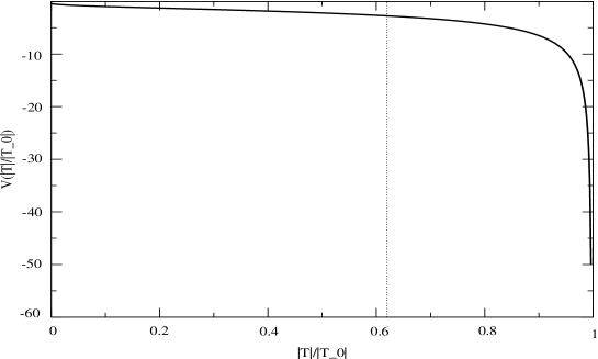
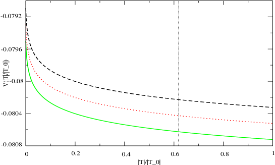
As has been pointed out earlier, since $m$ denotes the ADM mass of a single $D6$-brane, we may demand $ml^{-1}_{s}\geq 1$ in order for our supergravity description to be valid. (It should be clear, from eq.(24), that both $m$ and $a$, in the natural unit, carry the dimensions of the length.) Then from eq.(42), it is obvious that for $m^{2}>3l^{2}_{s}$, then $m^{2}_{T}>0$ and for $0<m^{2}<3l^{2}_{s}$, $m^{2}_{T}<0$. This result indicates that for successful tachyon condensation in which tachyon mass squared has to become positive definite, we should demand $m^{2}>3l^{2}_{s}$, which is consistent with the condition for the supergravity description to be valid. Moreover, as the ratio $(m^{2}/l^{2}_{s})$ gets larger, which certainly is in the allowed region in the supergravity analysis, tachyon gets heavier and eventually the tachyon, rolled down to the minimum of its potential, would decouple, i.e., disappear from the spectrum of massless particles. And we identify this with a successful tachyon condensation. This behavior has been illustrated in Fig.2 where it can be seen that as the ratio $(m^{2}/l^{2}_{s})$ gets larger, the potential gets deeper implying that the quantity representing the effective tachyon mass squared, $d^{2}V/d|T|^{2}$ evaluated near the minimum of the potential gets bigger. In the mean time, for the other case $0<m^{2}<3l^{2}_{s}$, the tachyon mass squared is still negative definite and this may signal that although the tachyon condensation may proceed, some instability of the system still remains. It, however, is interesting to note that for this second case, we can, as a by-product, determine the true vev of the tachyon field at which the minimum of the potential occurs. That is, taking $m\simeq l_{s}$, the tachyon mass squared becomes

$$m^{2}_{T}\simeq-{4l_{s}\over|T_{0}|^{2}}.$$ (41)

Finally, comparing this with its genuine stringy counterpart, $m^{2}_{T}=-1/\alpha^{\prime}$ leads us to determine the true vev of the open string tachyon field as

$$|T_{0}|=2l^{3/2}_{s}.$$ (42)

Namely, the minimum of the open string tachyon potential $V(|T_{0}|)=-2m$ occurs when the vev of tachyon takes value of the order $l^{3/2}_{s}$.
Lastly, with the supergravity analogue of tachyon potential $V(|T|)$ at hand, one might wish to determine the typical form of the spacetime dependent tachyon field profile $T(x)$. We now turn to this issue. Since the tachyon arising in a $D_{p}-\bar{D}_{p}$ system ($p=6$ in our case) is complex (and scalar for the single $N=1$ brane-antibrane case), we write $T(x)=|T(x)|e^{i\theta(x)}$. Then extremizing the tachyon action

$$S_{T} = -{T_{9}\over\sqrt{\alpha^{\prime}}}\int d^{10}x[\partial_{\mu}T^{*}\partial^{\mu}T+V(|T|)]$$

$$= -{T_{9}\over\sqrt{\alpha^{\prime}}}\int d^{10}x\sqrt{\alpha^{\prime}}[\partial_{\mu}|T|\partial^{\mu}|T|+|T|^{2}\partial_{\mu}\theta\partial^{\mu}\theta+V(|T|)]$$

with respect to $|T(x)|$ and $\theta(x)$ respectively yields the following tachyon field equations

$$\partial_{\mu}\partial^{\mu}|T|-|T|\partial_{\mu}\theta\partial^{\mu}\theta+m^{2}l^{2}_{s}{1\over|T|}\left(m^{2}-l^{2}_{s}\ln{{|T|^{2}\over|T_{0}|^{2}}}\right)^{-3/2}=0,$$

$$\partial_{\mu}(|T|^{2}\partial^{\mu}\theta)=|T|^{2}\partial_{\mu}\partial^{\mu}\theta+2|T|\partial_{\mu}|T|\partial^{\mu}\theta=0.$$ (44)

Now, since the true vacuum to which the tachyon condenses is $V(|T_{0}|)=-2m$ at which $|T|=|T_{0}|=2l^{3/2}_{s}$, we look for a finite action solution to these field equations which asymptotes to $|T_{0}|$ at $|x|\rightarrow\infty$. From the second equation, it is rather obvious that the most naive solution involves $\theta(x)=constant$ in which case the first equation reduces to

$$\partial_{\mu}\partial^{\mu}|T|+m^{2}l^{2}_{s}{1\over|T|}\left(m^{2}-l^{2}_{s}\ln{{|T|^{2}\over|T_{0}|^{2}}}\right)^{-3/2}=0$$ (45)

while the next simplest solution would involve $\partial^{\mu}\theta(x)=c^{\mu}/|T|^{2}$ (where $c^{\mu}$ is a constant vector normalizable to $c^{\mu}c_{\mu}=l^{4}_{s}$) in which case the first equation becomes

$$\partial_{\mu}\partial^{\mu}|T|-{l^{4}_{s}\over|T|^{3}}+m^{2}l^{2}_{s}{1\over|T|}\left(m^{2}-l^{2}_{s}\ln{{|T|^{2}\over|T_{0}|^{2}}}\right)^{-3/2}=0.$$ (46)

These equations may be solved analytically or at least numerically. We may have more to say on this in our future work.

4 Summary and discussions

To summarize, in this work, using an exact supergravity solution representing the $D6-\bar{D6}$ system, we demonstrated in a rigorous fashion that one can construct a supergravity analogue of the tachyon potential which may possess generic features of the genuine stringy tachyon potentials. In doing so, our philisophy was to evaluate the interaction energy between the brane and the antibrane for small but finite inter-brane separation and then identify it with the tachyon potential $V(T)$. And this identification demands an appropriate suggestion to relate the parameter $a$ in the supergravity solution representing the inter-brane distance to the tachyon field expectation value and we proposed an ansatz given in eq.(31). For the tachyon potential thus obtained, its minimum value was of particular interest in association with Sen’s conjecture for the tachyon condensation on unstable $D$-branes in type II theories. In the absence of the magnetic field (i.e., $RR$ $F7$-brane) content, minimum of the potential was unbounded below and it is due to the Coulomb-type combined gravitational and gauge attractions between the brane and the antibrane when they are close enough to each other. Then by introducing the magnetic field content with an appropriate strength $B$ removing all the conical singularities of the $D6-\bar{D6}$ solution, the tachyon potential has been regularized, i.e., made to be bounded below. Remarkably, now the finite minimum value of the potential turned out to be $V(T_{0})=-2m$. Since $m$ denotes the ADM mass of a single $D6$-brane, this result, in a sense, appears to confirm that Sen’s conjecture is indeed correct although the analysis used is semi-classical in nature and hence should be taken with some care. Also commented was the fact that the supergravity analogue of the tachyon potential constructed in the present work can only be that in the $D_{p}-\bar{D}_{p}$ system and we need some other approach to obtain the tachyon potential in the other non-BPS $D_{p}$-branes, i.e., the $D_{p}$-branes with “wrong” $p$. We also read off, from the vanishing separation (between $D6$ and $\bar{D6}$) limit of the supergravity analogue of the tachyon potential, the value of the supergravity analogue of the tachyon mass squared $m^{2}_{T}$. Then we demonstrated that the quantity $m^{2}_{T}$ (which has started out as being negative) can actually become positive definite as the tachyon rolls down toward the minimum of its potential. It indeed signals the possibility of successful condensation of the tachyon since it shows that near the minimum of its potential, tachyon can become as heavy as desired within the validity of supergravity description and disappear from the spectrum. Lastly, we provided tachyon field equations from which one can determine, as a solution, the spacetime dependent tachyon field profile $T(x)$.
It is also interesting to note that lately, motivated by the series of suggestions made by Sen [20], some intriguing possibility of tachyonic inflation on unstable non-BPS branes has been proposed and explored [21] . There, the tachyon field, whose dynamics on a non-BPS brane is described by an extended version of Dirac-Born-Infeld (DBI) and Chern-Simons (CS) action terms containing both the kinetic and potential energy terms for the tachyon field, plays the role of “inflaton” driving an inflationary phase on the brane world. Clearly, the most crucial condition for the occurrence of “slow roll-over” regime in a new inflation-type model is the nearly flat structure of the tachyon potential. Tachyon potential with such highly restricted behavior has not been available when looked for in the context of the open (super) string field theory constructions [7]. In this sense, it is quite promising that the supergravity analogue of the tachyon potential obtained in the present work can serve as a successful candidate for such a flat potential since, as we have seen in this work, it possesses purely logarithmic dependence on the tachyon field and hence is slowly varying. Thus it will be the issue of one of our future works to explore the potentially successful role played by the tachyon field arising in the unstable $D_{p}-\bar{D}_{p}$ system and having the structure of potential discovered in the present work.
After all, having a closed form for a tachyon potential at hand invites a lot of opportunity to explore many exciting issues in string/brane physics and its cosmological implications. It is our hope that here we actually have made one step further in this direction.

References

- [1] O. Bergman and M. R. Gaberdiel, Phys. Lett. B441 (1998) 133 ; A. Sen, JHEP 9809 (1998) 023 ; JHEP 9810 (1998) 021 ; JHEP 9812 (1998) 021 ; E. Witten, JHEP 9812 (1998) 019 ; P. Horava, Adv. Theor. Math. Phys. 2 (1999) 1373.
- [2] J. A. Harvey, P. Horava and P. Krauss, JHEP 0003 (2000) 021 ; M. R. Gaberdiel, Class. Quant. Grav. 17 (2000) 3483.
- [3] A. Lerda and R. Russo, Int. J. Mod. Phys. A15 (2000) 2000.
- [4] M. Frau, L. Gallot, A. Lerda and P. Strigazzi, Nucl. Phys. B564 (2000) 60 ; L. Gallot, A. Lerda and P. Strigazzi, Nucl. Phys. B586 (2000) 206 ; M. Bertolini, P. Di Vecchia, M. Frau, A. Lerda, R. Marotta, and R. Russo, Nucl. Phys. B590 (2000) 471.
- [5] K. Bardakci, Nucl. Phys. B68 (1974) 331 ; K. Bardakci and M. B. Halpern, Phys. Rev. D10 (1974) 4230 ; K. Bardakci and M. B. Halpern, Nucl. Phys. B96 (1975) 285 ; K. Bardakci, Nucl. Phys. B133 (1978) 297.
- [6] A. Sen, JHEP 9808 (1998) 010 ; JHEP 9808 (1998) 012 ; JHEP 9912 (1999) 027 ; hep-th/9904207.
- [7] E. Witten, Nucl. Phys. B268 (1986) 253 ; V. A. Kostelecky and S. Samuel, Phys. Lett. B207 (1988) 169 ; Nucl. Phys. B336 (1990) 263 ; A, Sen and B. Zwiebach, JHEP 0003 (2000) 002 ; N. Berkovits, A. Sen and B. Zwiebach, Nucl. Phys. 587 (2000) 147 ; N. Berkovits, JHEP 0004 (2000) 022 ; N. Moeller, A. Sen and B. Zwiebach, JHEP 0008 (2000) 039 ; N. Moeller and W. Tayler, Nucl. Phys. B583 (2000) 105 ; J. A. Harvey and P. Krauss, JHEP 0004 (2000) 012 ; R. de Mello Koch, A. Jevicki, M. Mihailescu and R. Tatar, Phys. Lett. B482 (2000) 249.
- [8] Ulf H. Danielsson, A. Guijosa and M. Kruczenski, JHEP 0109 (2001) 011.
- [9] K. Hashimoto, JHEP 0207 (2002) 035.
- [10] A. Sen, JHEP 9710 (1997) 002.
- [11] D. Gross and M. Perry, Nucl. Phys. B226 (1983) 29.
- [12] W. B. Bonnor, Z. Phys. 190 (1966) 444 ; S. Mukherji, hep-th/9903012 ; B. Janssen and S. Mukherji, hep-th/9905153.
- [13] R. Emparan, Phys. Rev. D61 (2000) 104009 ; A. Chattaraputi, R. Emparan and A. Taormina, Nucl. Phys. B573 (2000) 291.
- [14] A. Davidson and E. Gedalin, Phys. Lett. B339 (1994) 304 ; D. V. Galtsov, A. A. Garcia and O. V. Kechkin, Class. Quant. Grav. 12 (1995) 2887.
- [15] D. Youm, Nucl. Phys. B573 (2000) 223.
- [16] F. J. Ernst, J. Math. Phys. 17 (1976) 515.
- [17] P. Brax, G. Mandal and Y. Oz, Phys. Rev. D63 (2001) 064008.
- [18] Y. C. Liang and E. Teo, Phys. Rev. D64 (2001) 024019.
- [19] S. W. Hawking and G. T. Horowitz, Class. Quant. Grav. 13 (1996) 1487.
- [20] A. Sen, hep-th/0203211 ; hep-th/0203265 ; hep-th/0204143.
- [21] G. W. Gibbons, hep-th/0204008 ; M. Fairbairn and M. H. G. Tytgat, hep-th/0204070.