Large-momentum convergence of Hamiltonian bound-state dynamics of effective fermions in quantum field theory

Abstract

Contributions to the bound-state dynamics of fermions in local quantum field theory from the region of large relative momenta of the constituent particles, are studied and compared in two different approaches. The first approach is conventionally developed in terms of bare fermions, a Tamm-Dancoff truncation on the particle number, and a momentum-space cutoff that requires counterterms in the Fock-space Hamiltonian. The second approach to the same theory deals with bound states of effective fermions, the latter being derived from a suitable renormalization group procedure. An example of two-fermion bound states in Yukawa theory, quantized in the light-front form of dynamics, is discussed in detail. The large-momentum region leads to a buildup of overlapping divergences in the bare Tamm-Dancoff approach, while the effective two-fermion dynamics is little influenced by the large-momentum region. This is illustrated by numerical estimates of the large-momentum contributions for coupling constants on the order of between 0.01 and 1, which is relevant for quarks.

I Introduction

The notion of a bound state of fermions is based mainly on the examples of atoms and nuclei. The common feature of these systems is that they are non-relativistic. This means three things. Kinetic energies of the fermions are small in comparison to their rest mass energy. Dominant interactions are not able to produce fast moving fermions from the slow ones and hence no significant large-momentum spin effects are generated. Creation of additional particles can be neglected and one can describe the bound states as built from a fixed number of fermion constituents. These features are all related to the fact that the domain of large relative momenta is not important, which is easiest to describe in mathematical terms in the case of bound states of two fermions, such as positronium or deuteron. Their wave functions are self-consistent solutions to the non-relativistic Schrödinger equation $H|\Psi\rangle=E|\Psi\rangle$ with Hamiltonian $H=H_{0}+H_{I}$, where $H_{0}$ denotes the kinetic energy operator and $H_{I}$ stands for the interaction operator. The matrix element $\langle 12|H_{I}|1^{\prime}2^{\prime}\rangle$ is the quantum Coulomb, or Yukawa potential with a repulsive core, respectively. The ket $|12\rangle$ denotes a state of two fermions labeled 1 and 2, with all their quantum numbers collectively denoted by these labels. The self-consistency of this well known picture means that the wave function $\psi(1,2)=\langle 12|\Psi\rangle$ quickly vanishes when the relative momentum of fermions in the bound-state rest frame of reference, $\vec{p}=\vec{p}_{1}-\vec{p}_{2}$, approaches values comparable with the fermions’ reduced mass $\mu$ (the speed of light, $c=1$).

The success of the Schrödinger picture for bound states of fermions extends also to quarks. This is reflected in the constituent quark model (CQM) being the primary means for classification of hadrons in the particle data tables, and providing a benchmark for more advanced approaches. However, the self-consistency of the non-relativistic picture is much harder to maintain for bound states of quarks up, down, and strange, than for systems such as positronium and deuteron. This is because the hadronic wave functions tend to have considerable components with $|\vec{p}\,|$ comparable to or exceeding $\mu$ for the quarks, and the domain of large relative momenta begins to play a significant role in the binding mechanism. One is also interested in the description of hadrons moving with speeds very close to the speed of light. Since the fast moving hadrons and their interactions cannot be consistently described within a purely non-relativistic Schrödinger framework, theorists use the Feynman parton model in that case. Unfortunately, the binding mechanism of partons is far beyond the scope of the parton model. As alternative to these models, one can approach the issue of bound states of fermions using quantum field theory (QFT), where the corresponding operator $H$ appears to contain all the relevant information about relativistic effects in the domain of large relative momenta of the constituents.

However, the relativistic description of bound states of fermions in QFT, especially in quantum chromodynamics (QCD) in the case of light quarks, makes the conceptual difficulties with the constituent picture even greater than in the simple models. In the equation $H_{QCD}|\Psi\rangle=E|\Psi\rangle$, all factors remain unknown. Major reasons for this status of the theory originate in the large relative momentum domain in the motion of virtual particles. This is illustrated by the following examples. One is that local QFTs lead to canonical interaction Hamiltonians $H_{I}$ that change individual bare particle energies by unlimited amounts (spin-dependent factors grow with momentum transfers). The large momentum range is enhanced and leads to divergences, invalidating the concept of a non-relativistic picture entirely unless special conditions, such as an extraordinarily small coupling, are met. Another example is that the interactions create new bare particles and this effect contributes to the boosting of bound states, which implies that the motion of bound states is associated with multi-particle components and the ad hoc limitation to a fixed number of bare constituents goes out the window in relativistic QFTs. A third example is that even the state with no constituent particles, i.e. the ground state of a theory, or vacuum, proves to be so complicated that no approximate solution of verifiable accuracy has been conceived yet, although many ansatzes have to be and are employed in practical attempts. In these circumstances, the main theoretical approach to bound states of quarks (mainly heavy ones that move slowly) is based on the lattice version of QCD, and great progress has been achieved in numerical studies of the theory that way. Nevertheless, it appears that a quantitative explanation of how the constituent picture with a simple Hamiltonian could be an approximate solution, remains a conceptual and quantitative mystery. No detailed constituent wave function picture for relativistic field quanta in Minkovsky space has been theoretically identified or is expected to readily follow from the lattice approach alone. The question of convergence of the binding mechanisms in the domain of large relative momenta of constituent particles, remains open.

This article provides some numerical arguments that the required constituent picture with well-controlled large relative momentum domain may become in principle identifiable if one provides a precise definition of the constituents as effective particles, in distinction from the bare quanta of the local theory. Thus, the process of solving a theory is arranged in two steps, which is typical in lattice approach lattice , or sum rules SVZ . In the first step, one derives an effective dynamics, and, in the second step, one attempts to solve the effective theory instead of dealing directly with the original degrees of freedom. Here, one derives the effective fermions of size $\lambda^{-1}$ using a suitable boost-invariant perturbative renormalization group procedure for their Hamiltonians. The procedure is carried out up to second-order perturbation theory, and the resulting dynamics is compared with the standard picture, where the finite scale $\lambda$ is absent. In distinction from the diverging bare dynamics, the effective one comes out limited to the momentum range given by $\lambda$, and this scale is reduced using differential equations to the most suitable one for description of bound state properties in terms of a fixed number of the corresponding constituents. In the renormalized Hamiltonian picture, the point-like bare particles of the local theory correspond to $\lambda=\infty$ and their dynamics heavily involves large momenta, and multi-particle states, for any finite value of the coupling constant. However, the situation is completely changed when $\lambda$ is lowered to values comparable to the bound state masses. The binding is described by a new Schrödinger equation, $H_{\lambda}|\Psi\rangle=E|\Psi\rangle$, where the Hamiltonian, $H_{\lambda}=H_{0\lambda}+H_{I\lambda}$, is written in terms of creation and annihilation operators for the effective particles, $b^{\dagger}_{\lambda}$ and $b_{\lambda}$ for fermions, $d^{\dagger}_{\lambda}$ and $d_{\lambda}$ for anti-fermions (and $a^{\dagger}_{\lambda}$ and $a_{\lambda}$ for bosons). This effective particle picture is discussed in the present paper.

The key physical reasons for the hope that the effective constituent picture does emerge from QFT can be understood by recalling again what happens in the well-known cases of atoms (or positronium) and nuclei (or deuteron) discussed above. These systems can be understood in terms of constituents for quite different reasons. The explanation of the difference is limited below to the positronium and deuteron, but the two examples are sufficient to make the point that concerns all bound systems of fermions in QFT. In the Schrödinger quantum-mechanical picture of positronium, the coupling constant that appears in the Coulomb potential is very small in comparison to 1, i.e. $e^{2}/4\pi=\alpha\sim 1/137$. Therefore, the interaction produces quite small binding energy, of order $\alpha^{2}\mu/2$, and the $e^{+}e^{-}$ bound-state mass is dominated by $2m_{e}$. The relative-motion wave function is proportional to $(\alpha^{2}\mu^{2}+|\vec{p}\,|^{2})^{-2}$, independently of the fermion spins. When one extends this picture by embedding it in quantum electrodynamics (QED), one finds out that the initial wave function is so small for large momenta $\vec{p}$, that no significant correction is able to emerge from that region and alter the original picture with the Coulomb potential. This is found by expanding the theory term by term in powers of $\alpha$ around the initial Schrödinger picture. The interaction linear in $\alpha$ (Coulomb force) is sufficient to describe the main features of fermionic bound states in QED, and higher powers of $\alpha$ are not important for theoretical understanding of the bulk of the bound state structure. Although the integrals in the corrections run over the momentum range that formally extends far beyond $\mu$, the coupling constant is too small for the relativistic fermion spin factors and particle creation processes to produce any major modifications of the leading approximation. This feature will be farther discussed in the next Sections.

In the meson-exchange models of the deuteron binding mechanism, the analogous coupling constant is three orders of magnitude larger than in QED. If one attempted to use QFT to derive the Yukawa potential using the same strategy as in QED, and to calculate corrections, the perturbative procedure would fail. The interactions would accelerate nucleons to the speed of light almost immediately on the bound-state formation time-scale, many new particles would be created, and the large momentum relativistic “corrections” would dominate the “leading” non-relativistic terms. One could then ask why the famous one-boson-exchange (OBE) potentials, such as the Yukawa potential with a core, could still be used in phenomenology of relativistic nuclear physics and work self-consistently in the nuclear bound-state equations anyway. What saves the picture of a fixed number of relatively slow nucleons interacting through exchange of mesons from serious inconsistency when one includes the elements of QFT, is that the interactions responsible for emission and absorption of mesons by nucleons contain form factors that limit momentum transfers to values so small that the interactions are effectively weak, much weaker than a change of $\alpha$ in QED by the factor 1000 would imply. Consequently, the binding energy is much smaller than the sum of two nucleon masses, e.g. about 2.2 MeV for deuteron. The wave functions of such generalized relativistic nuclear physics picture are not overwhelmingly extending into the large-relative-momentum domain because the form factors eliminate coupling to that region and the non-relativistic Yukawa potential with a repulsive core is not invalidated by huge corrections. It could not be so with bare point-like fermions in local QFT, but it does work in the phenomenological picture of effective particles with the form factors. By the way, this example is not intended to suggest that nucleon dynamics should be completely derivable directly from a local QFT that ignores the existence of quarks. In fact, a scenario for how to derive the effective nuclear physics picture from QCD will be discussed in the last Section of this work. Nevertheless, the nuclear physics picture does indicate that an effective particle dynamics may involve large coupling constants in potentials that resemble perturbative second-order interactions with form factors.

In QCD, none of the two schemes can apply separately. On the one hand, the effective coupling constant in the constituent QCD picture cannot be as small as in QED, because QCD is characterized by asymptotic freedom, or infrared slavery. This means that the effective coupling strength is expected to grow when the scale of relevant momentum transfers decreases. The coupling constant is already on the order of 0.1 at transfers on the order of 100 GeV and it may be much larger for transfers on the order of nucleon masses. Therefore, the effects that have marginal size in the eigenvalue problem for approximate $H_{QED}$, such as spin splittings, are expected to be much larger and more important for understanding eigenstates of $H_{QCD}$, and the initial approximation is not as simple as in QED. On the other hand, one cannot freely insert form factors into the local Lagrangian for quark and gluon fields because it would spoil the local gauge symmetry structure. The contact with QCD would be irreversibly lost.

The situation is changed when QFT is approached using the idea of similarity renormalization group procedure for Hamiltonians sim1 , especially in the case of QCD KWetal , and when one combines the similarity idea with the concept of form factors in the Hamiltonian interaction vertices for effective particles Gacta . Initially, the coupling constant is small due to asymptotic freedom and one can think of using the small coupling constant in canonical QFT to solve the renormalization group equations for $H_{\lambda}$ using a perturbative expansion. The method avoids small energy denominators in the perturbative calculation entirely and the non-perturbative part of the dynamics remains untouched in the perturbative calculation of $H_{\lambda}$. That way one derives effective-particle Hamiltonians that involve vertex form factors of small width $\lambda$ in the interaction terms. One can have sizable couplings in $H_{\lambda}$ with small $\lambda$, as required by infrared slavery, without losing control over the size of corrections to the leading constituent picture in diagonalizing $H_{\lambda}$. The spectrum of such Hamiltonians can be sought numerically because the form factors limit the range of momenta strongly enough for a discrete computer code to cover the pertinent region, as in the nuclear physics case discussed above. This idea has already been studied qualitatively in a simple numerical matrix model GWafbs using Wegner’s flow equation Wegner (and its generalizations). The more detailed effective particle calculus used in the present work in the case of Yukawa theory, is already known to produce asymptotic freedom in $H_{\lambda}$ for QCD Ggluon . The new approach has been also extended to the whole Poincaré algebra poincare in QFT.

The present paper provides elementary numerical estimates of the orders of magnitude of the interactions that appear in QFT in the bound state dynamics of two effective fermions of size $\lambda^{-1}$. Yukawa theory is used to avoid complications related to gauge symmetry while one still preserves some of the singular large-momentum components in the spinor factors that characterize fermions. The well-known issue of triviality in Yukawa theory is irrelevant here since our goal is to estimate the size of corrections in the bound-state dynamics in an effective theory, rather than in the ultra-violet (UV) dynamics of the initial QFT. The Yukawa example serves only as a source of typical UV factors that QFTs provide anyway, no matter if the theory is trivial, asymptotically free, or otherwise.

The key qualitative question is by how much the Hamiltonian $H_{\lambda}$ derived in QFT might differ from familiar models, especially from the non-relativistic Schrödinger picture with a Yukawa potential (or a Coulomb potential in the case of exchange of massless mesons), for given values of $\alpha$ and $\lambda$. Another question is related to the fact that the exact solution of renormalization group equations for $H_{\lambda}$ and subsequent exact diagonalization of $H_{\lambda}$ should lead to spectra that are independent of $\lambda$. However, when one calculates $H_{\lambda}$ in perturbation theory of low order, such as the second order that characterizes the Coulomb and Yukawa potentials, the $\lambda$-dependence must appear. Bound-state energies may depend on $\lambda$ when $\lambda$ is made too small or $\alpha$ is made too large. The question is how large is the residual $\lambda$ dependence of second-order corrections to the Coulomb-like picture in how large a range of values of $\alpha$ and $\lambda$ that can be self-consistently (i.e., without significant $\lambda$-dependence) reached in lowest orders of perturbation theory, for $H_{\lambda}$ itself in the renormalization group part of the calculation, and for the eigenvalues and wave functions in the bound state perturbation theory around the Coulomb-like ansatz. Both questions are answered in the next Sections by estimating the size of those corrections that are most important for large momenta, and which would lead to divergences in the absence of $\lambda$. The results imply that the most dangerous corrections that might diverge in the absence of $\lambda$, turn out to be quite small even for sizable coupling constants. This provides some initial ground for the hope that the effective particle dynamics can be attempted numerically in QCD in the same way. An outline of how the same approach, if successful, could then in principle also lead from effective $H_{\lambda QCD}$ to the effective meson-exchange interactions between nucleons in nuclear physics, is also provided.

Many farther dynamical issues of great interest, concerning effective fermions and their binding in QFT, can be posed and investigated using the effective particle calculus, but none are studied here in detail. For example, the case of phonon exchange between electrons as approximated by a QFT is not discussed here WPR , and symmetry restoration issues in not-explicitly symmetric Hamiltonian approach through coupling coherence PPR is also not considered. Instead, this work is focused on the readily accessible quantitative estimates that show the magnitude of the difference between the convergent two-effective fermions bound-state dynamics and the diverging dynamics of two bare fermions in the approaches based on the Tamm-Dancoff truncation in local QFT tamm ; dancoff . In fact, this paper starts with the Tamm-Dancoff-like approach to local theory, because it is more familiar. Then, the effective particle approach is introduced, with its new features exposed through the contrast with the Tamm-Dancoff one. Thus, Section II provides definitions of the renormalized Tamm-Dancoff scheme in Subsection II.1, and the effective particle scheme in Subsection II.2. Both approaches involve a universal procedure for obtaining a two-fermion eigenvalue equation that can be compared with the non-relativistic Schrödinger equation. This universal procedure is for brevity called reduction. It is denoted by the symbol $R$ and described in subsection II.3. Section III introduces a bare light-front Hamiltonian in Yukawa quantum field theory that serves as a starting point for subsequent Sections. The canonical Hamiltonian is supplied with some regularization factors $r_{\Delta}$ and counterterms. Section IV describes details of the approach that treats bound states of fermions as if they could be viewed as made of two bare fermions. This approach is shortly called approach 1 and encounters large-momentum conceptual and calculational difficulties that are removed by switching over to the approach discussed in detail in Section V. Namely, Section V presents the effective fermion approach, called approach 2, using comparison and contrast with the approach 1. In the approach 2, bound states of fermions are treated as built from effective fermions of size $\lambda^{-1}$. Conclusions are drawn in Section VI. Appendixes contain information about the operation $R$, spinor factors, momentum variables, and a Coulomb bound state wave function used in the calculations.

II Definitions

This Section provides definitions of two light-front Hamiltonian approaches to the bound state dynamics, the renormalized Tamm-Dancoff approach (approach 1), and effective particle approach (approach 2). They are compared through numerical estimates in next Sections in the case of a bound state of two fermions. The procedure of reducing a theory to the two-fermion sector is mathematically the same in both cases, except for a different definition of what is meant by the two-fermion states. In the approach 1, the starting point will be identical with bare fermions in QFT, in the approach 2 it will be the effective ones. The reduction procedure, denoted by $R$, is described at the end of this Section for both approaches simultaneously.

II.1 Renormalized Tamm-Dancoff approach

This approach is represented by the following diagram,

$${\cal L}\,\,\stackrel{{\scriptstyle 0}}{{\rightarrow}}\,\,:H_{can}:\,\,\stackrel{{\scriptstyle i}}{{\rightarrow}}\,\,:H_{can}^{\Delta}:+X^{\Delta}\,\,\stackrel{{\scriptstyle ii}}{{\longleftrightarrow}}\,\,\rm{solve}\,\,.$$ (1)

0) The initial step on the left denotes a canonical derivation of a field theory Hamiltonian from its Lagrangian, quantization, and normal ordering with respect to the bare vacuum state, dropping all diverging terms on the basis of hindsight knowledge that the normal ordered Hamiltonian will eventually contain counterterms of the same structure, but well defined.

i) The next step is called regularization, which is necessary because the canonical Hamiltonian leads to ultraviolet divergences due to the infinite range of energy scales to sum over in the intermediate states when one calculates physical observables (such as scattering cross-section) using perturbative formulae. One imposes an ultraviolet cutoff (we denote it by $\Delta$) on the range of momenta that are included in the sums. Observables calculated with such regularized Hamiltonian explicitly depend on both the parameter $\Delta$, and on the way the regularization is imposed. For example, the regularization may preserve or violate some symmetries - an oblate cutoff function would not be rotationally symmetric, or a frame-dependent cutoff would not respect Lorentz symmetry, and finite corrections due to such regularizations would be required. To remove the artificial dependence of observables on regularization, one has to add new terms to the Hamiltonian (called counterterms and denoted $X^{\Delta}$) that also depend on the regularization. The construction of counterterms is based on the idea of recovering the contribution from dynamics above the cutoff, which is to lead to finite and cutoff independent results when $\Delta\rightarrow\infty$. The counterterms structure is thus determined by the structure of divergences. The latter can be computed and $X^{\Delta}$ is than adjusted to cancel the cutoff dependence. It is less straightforward to remove finite effects of regularization, but this issue will not be important in the next Sections. The regularized Hamiltonian $:H_{can}^{\Delta}:+X^{\Delta}$ is denoted by $H^{\Delta}$.

ii) The last arrow indicates solving of the eigenvalue equation for $H^{\Delta}$. A two-steps procedure is used.

Step a) First one finds eigenstates of $H^{\Delta}$ whose dominant component for vanishingly small coupling constants is equal to one bare fermion. These states represent what one could call a physical fermion. The solution is found from the eigenvalue equation for the whole $H^{\Delta}$ by reducing that equation with the help of operation $R$ to an equivalent equation for the Fock component with one bare fermion. If one requires the eigenvalue to be finite, one has to include in $X^{\Delta}$ a mass counterterm of a calculable form.

Step b) Then, one makes a reduction $R$ of the eigenvalue problem for $H^{\Delta}$ to a two-bare-fermion subspace, to find an eigenstate of the Hamiltonian $H^{\Delta}$ that is dominated by a pair of bare fermions for infinitesimally small coupling constants. The parameters in the resulting two-fermion eigenvalue problem are expressed in terms of the physical fermion mass found in step a) above. It turns out that the calculated eigenvalues still depend on the cutoff (some diverge if $\Delta\rightarrow\infty$), although the individual matrix elements of the reduced two-body Hamiltonian do not depend on the cutoffs once one includes mass counterterms calculated in ii a). Therefore, there is a problem of how to construct counterterms that would remove $\Delta$ dependence from physical results pinsky .

It is important to mention here an alternative approach, which is also inspired by the Tamm-Dancoff truncation but includes renormalization group idea in a more sensible way Perry:mz . Namely, one can assume that some effective fermion representation of the eigenstates of $H^{\Delta}$ does exist. One tries then to build a triangle of renormalization (the notion of the triangle in the case of similarity renormalization group scheme for light-front Hamiltonians can be found in Ref. KWetal ) for a sequence of calculations with growing cutoffs $\Delta$ and growing numbers of fermions and bosons, adjusting counterterms to the momentum cutoffs differently in different Fock sectors. The hope is to understand regularities in the obtained structures that produce stable outputs when the momentum cutoffs and the particle numbers are made so large in the triangle that one can follow the renormalization group flow down from the large values and recognize interactions that have a universal character. Moving then along the renormalized Hamiltonian trajectory in the triangle, one would be able to arrive at the desired effective particle picture. One of the key tools one would use in studying the triangle would be the coupling coherence PPR that requires that the interactions retain their forms when one moves around the triangle with large values of the cutoffs. This approach is thus relying on regularities that need to be discovered in a vast amount of intricate analytic and numerical data. The data can also be interpreted with the help of perturbative techniques wherever possible. As a variation of this idea, one may even attempt to include new degrees of freedom, such as Pauli-Villars pseudo-particles, and treat them as a suitable way of writing down required counterterms zle . However, the latter strategy faces a problem of sending the regulator masses to infinity (it is not clear how to do it using computers) or living with the additional degrees of freedom that are absent in the initial theory. One also uses discretization of the longitudinal light-front momenta (usually denoted by $p^{+}$) casher , which limits the number of constituents. However, the transverse dynamics is not smoothed out that way and poses the same divergence problems. The initially helpful longitudinal cutoff has to be relaxed in order to recover boost invariance. At that stage, the same problems reappear fully again and remain unsolved. Thus, the already known options for general searches for effective fermion dynamics are hard to pursue. In contrast, in the present article, it is taken for granted that one can assume from the very beginning a large degree of rigidity in the derivartion of effective theory by writing it in terms of creation and annihilation operators for effective particles. The assumption allows one to narrow the search for effective dynamics using a unitary renormalization group procedure Gacta , which is the basis for the approach 2 introduced below.

II.2 Renormalized effective particle approach

The procedure consists of three steps that are described later in detail in Section V, and can be represented by the following diagram.

$${\cal L}\,\,\stackrel{{\scriptstyle 0}}{{\rightarrow}}\,\,:H_{can}:\,\,\stackrel{{\scriptstyle i}}{{\rightarrow}}\,\,:H_{can}^{\Delta}:+X^{\Delta}\,\,\stackrel{{\scriptstyle U_{\lambda}}}{{\longleftrightarrow}}\,\,H_{\lambda}\stackrel{{\scriptstyle iii}}{{\rightarrow}}\rm{solve}$$ (2)

The steps 0) and i) are the same as before except that one works with the bare creation and annihilation operators for efficient book-keeping for Hamiltonian terms at all times, instead of storing a huge number of selected matrix elements of $H^{\Delta}$. Note that many other operators could have the same selected matrix elements. Also, matrix elements of operators change when the basis states change even if the operators remain unchanged, and the same operator may have different matrix elements when different states are used to represent constituent particles.

ii) This step, marked with $U_{\lambda}$ in the diagram, is made using the procedure of renormalization group for effective particles (RGEP) Gacta ; Ggluon . The procedure is defined as a unitary rotation of creation and annihilation operators by an operator $U_{\lambda}$. Hamiltonians $H_{\lambda}$ are expressed in terms of the effective-particle creation and annihilation operators that depend on the “width” parameter $\lambda$. $\lambda$ ranges from $\infty$ in $H^{\Delta}$ to a finite value on the order of bound-state masses in the effective constituent dynamics. That such small scales can in principle be reached using perturbation theory GWafbs , is possible because RGEP procedure is designed according to the rules of the similarity renormalization group for Hamiltonians sim1 . It separates the perturbative from non-perturbative aspects of the theory (see the original articles). By the same design, the Hamiltonian $H_{\lambda}$ cannot change invariant masses of effective-particle Fock states by more than about $\lambda$ in a single interaction.

Figure 1: The main difference between $H^{\Delta}$ and $H_{\lambda}$ is that the latter is for effective particles of size $\lambda^{-1}$, instead of the point-like bare ones that the former is for, and interaction terms in $H_{\lambda}$ are limited by form factors $f_{\lambda}$. The form factors are marked in figures by a black blob.

Thus, the emission of effective bosons by effective fermions is possible only if the associated kinetic energy change of relative motion of the particles does not exceed $\lambda$. Consequently, when $\lambda$ is small, Fock sectors with different numbers of effective particles are coupled weakly even for sizable coupling constants, like in the nuclear physics example discussed in the Introduction.

iii) This step is analogous to the step ii) in the approach 1 and amounts to solving the eigenvalue problem for effective Hamiltonian $H_{\lambda}$. The key difference, however, is that when one works using the basis of effective particles in the Fock space, states with two effective fermions couple only to states with similar relative momenta. Therefore, the large relative momentum domain remains suppressed, and it can be described using perturbation theory without assuming that the coupling constant is very small. Thus, when one solves the eigenvalue equation for $H_{\lambda}$, one can introduce a new perturbation theory for the reduction operator $R$, expanding in powers of $H_{I\lambda}$. This gives an equivalent Hamiltonian that acts only in the dominant Fock space sectors. There are two steps to do, as in the approach 1.

In the step a), one first considers eigenstates dominated by one effective fermion, which defines a physical mass of a physical fermion in the approach 2. Then, in the step b), one finds an equation describing bound states of two effective particles. The parameter $\lambda$ is a key to the procedure. Its value determines whether derivation of the effective Hamiltonian $H_{\lambda}$ and its reduction by the operation $R$ to a model subspace Hamiltonian, denoted by $H_{R}$, is possible in perturbation theory. The smaller is $\lambda$ the simpler are the approximate solutions for bound states of effective fermions, in the sense that they tend to reduce to the dominant effective Fock sector. But if $\lambda$ is too small, the step ii) of derivation of $H_{\lambda}$ in perturbation theory loses accuracy (the perturbative integration of renormalization group equations begins to significantly cut into the bound-state dynamics). Therefore, $\lambda$ cannot be lowered too far using perturbation theory for $H_{\lambda}$. The optimal choice of $\lambda$ is the one that combines the simplest perturbative expansion for $H_{\lambda}$ with least complicated computer diagonalization of $H_{\lambda}$. The main criterion for choosing the right range for $\lambda$ is that the calculated observables are not sensitive to variation of $\lambda$ over that range.

The final comment concerns Refs. BP ; Jones , where a different concept of a bound state calculus has been developed using coupling coherence in second-order perturbation theory for Hamiltonian matrix elements, also in the similarity scheme but without the constraint to a boost-invariant unitary rotation of creation and annihilation operators (from the bare to effective ones). In distinction from these works, the approach 2 is not based on the coupling coherence because no coherent structure is known a priori in the region of small $\lambda$, far from the initial canonical structure. Instead, one uses a perturbative expansion for the effective-particle renormalization group flow in terms of a suitably defined coupling constant and tries to find out the relevant structures in a prescribed basis, in which the expansion in powers of the coupling constant may be extrapolable to its physical values. Here, the analysis of Yukawa theory is limited to numerical estimates of the size of only a few important terms of first and second order in a bound-state perturbation theory, which goes beyond the renormalization group flow. In the flow itself, it is already known that higher-order calculations are certainly possible even in much more complex theories (see e.g. Ggluon ). The effective bound-state dynamics is virtually unknown briprep .

II.3 Reduction procedure

The following scenario occurs several times in next Sections. There is an eigenvalue equation for a Hamiltonian $H=H_{0}+H_{I}$,

$$H|\psi\rangle=E|\psi\rangle\;,$$ (3)

which is too large to solve exactly on a computer in the sense that the number of a priori important basis states is infinite. One looks then for an equivalent Hamiltonian that acts only in a limited subspace of states. One way of constructing the model subspace dynamics is to use the transformation $R$ Bloch ; Wold . Details of the transformation are written in Appendix A. The idea is following.

One denotes the projection operator on the chosen subspace of the whole Fock space $F$ by ${\hat{P}}$, and the projector on the complementary space, $1-{\hat{P}}$, by ${\hat{Q}}$. If the interaction Hamiltonian $H_{I}$ is small in the sense that it only weakly couples states from the subspace $\hat{P}F$ to states in the subspace $\hat{Q}F$, then one can calculate an operator $R$ that produces certain eigenstates of $H$ from eigenstates of a new Hamiltonian $H_{R}$ that has eigenstates contained in the subspace $\hat{P}F$. The transformation $R$ leads to the following expression for the Hamiltonian $H_{R}$ acting in the subspace $\hat{P}F$, expanded in powers of the interaction Hamiltonian $H_{I}$ (cf. Eq. 36).

$$\langle i|H_{R}|j\rangle = \langle i|\left({\hat{P}}H{\hat{P}}+\frac{1}{2}{\hat{P}}H_{I}\frac{\hat{Q}}{E_{j}-H_{0}}H_{I}{\hat{P}}+\right.$$ (4)

$$\left.\frac{1}{2}{\hat{P}}H_{I}\frac{\hat{Q}}{E_{i}-H_{0}}H_{I}{\hat{P}}+\dots\right)|j\rangle\;.$$

Note that the Hamiltonian $H_{R}$ does not depend on the eigenvalues of $H$, but only on the eigenvalues of $H_{0}$. Namely, $H_{0}|i\rangle=E_{i}|i\rangle$. In particular, one can define $H_{0}$ in conjunction with the subspace $\hat{P}F$ so that $H_{I}=H-H_{0}$ is as weak as one can get simultaneously with preserving control over the spectrum of $H_{0}$. For example, in the case of two fermions, it is often useful to take $H_{0}$ equal to a sum of the kinetic energy and Coulomb potential operators when the fermions interact through emission and absorption of massless bosons with a small coupling strength. The strength of the coupling (size of $H_{I}$) may be small when the coupling constant itself is small, or when a form factor allows only small range of momentum transfers from the fermions to bosons and between the fermions.

III Canonical theory

We consider a theory of fermions of two kinds interacting through a Yukawa coupling with scalar bosons. The common starting point for all approaches to a two-fermion bound-state dynamics discussed in this paper is the Lagrangian:

$${\cal L}=\bar{\psi}(i\partial\!\!\!/-m-g\phi)\psi+\frac{1}{2}\partial_{\mu}\phi\partial^{\mu}\phi\;,$$ (5)

where $\bar{\psi}=\left(\bar{\psi}^{(1)},\bar{\psi}^{(2)}\right)$. That is, $\cal L$ includes the kinetic terms for two kinds of fermions (both of mass $m$), the kinetic term for massless scalar bosons and a point-like (Yukawa) interaction of the fermions with bosons.

The canonical Hamiltonian is defined using light-front quantization Yan , where the evolution of states in “time” $x^{+}=x^{0}+x^{3}$ is generated by a three-dimensional integral of the energy-momentum-density-tensor component $T^{+-}$ over the light-front hyper-plane $x^{+}=0$. The Hamiltonian is given by

$$P^{-}=\frac{1}{2}\int dx^{-}d^{2}x^{\perp}:\left[-\phi\partial^{\perp 2}\phi+\sum_{i=1}^{2}\left(\bar{\psi}_{m}^{(i)}\frac{-\partial^{\perp 2}+m^{2}}{i\partial^{+}}\gamma^{+}\psi_{m}^{(i)}+2g\phi\bar{\psi}_{m}^{(i)}\psi_{m}^{(i)}+g^{2}\bar{\psi}_{m}^{(i)}\phi\frac{\gamma^{+}}{i\partial^{+}}\phi\psi_{m}^{(i)}\right)\right]:\;.$$ (6)

$\psi_{m}$ are fermion fields that satisfy free Euler-Lagrange equations with mass $m$. Quantum commutation relations for all fields are satisfied by replacing all fields at $x^{+}=0$, [$x^{\perp}=(x^{1},x^{2})$ and $x^{-}=x^{0}-x^{3}$ are the “spatial” coordinates], by their Fourier expansions in terms of creation and annihilation operators (see Appendixes B and C for details). The canonical Hamiltonian derived this way leads to infinities in perturbative calculations of observables, due to summation over intermediate states with an infinite range of relative momenta that are reached by the local interactions from any state with only finite relative momenta. In order to regulate the Hamiltonian en bloc, including the binding mechanism, one has to introduce a cutoff $\Delta$ on the relative momenta in the interaction terms. The cutoff requires counterterms that remove the cutoff-dependence from observables in the limit $\Delta\rightarrow\infty$. Thus, the Yukawa-theory Hamiltonian takes the form

$$H^{\Delta}=H_{0}+H_{Y}^{\Delta}+H_{+}^{\Delta}+X^{\Delta}\;,$$ (7)

where $H_{0}$ denotes the contribution of the first two terms in Eq. (6), $H_{Y}$ of the third term, and $H_{+}$ of the fourth one. $X^{\Delta}$ represents the counterterms. To be specific, the relative momenta (see Appendix C for definitions of $x$ and $\kappa^{\perp}$) of created or annihilated particles are limited by inserting factors $r_{\Delta}=\exp{(-\kappa^{\perp 2}/\Delta^{2})}r_{\delta}(x)$ in the interactions terms, e.g. see Eq. (9). In the current study of Yukawa theory, the $x$-regulator factor $r_{\delta}(x)$ is needed only for the mass-counterterm construction. In all other formulae, it can be replaced by $1$. Since $r_{\delta}(x)$ does not appear in the final results, its form is left unspecified here (cf. Ggluon ).

The free part, $H_{0}$, is

$$H_{0} = \sum_{i,\sigma}\int[p]\frac{p^{\perp 2}+m^{2}}{p^{+}}\left(b^{(i)\dagger}_{p\sigma}b^{(i)}_{p\sigma}+d^{(i)\dagger}_{p\sigma}d^{(i)}_{p\sigma}\right)$$ (8)

$$+\int[p]\frac{p^{\perp 2}}{p^{+}}a^{\dagger}a\;.$$

There are three interaction terms. The one relevant here consists of emission and absorption of a boson by the fermions, i.e.

$$H_{Y}^{\Delta} = g\sum_{i,\sigma_{1},\sigma_{2}}\int\left[p_{1}p_{2}q\right]2(2\pi)^{3}\delta^{3}\left(p_{1}-p_{2}-q\right)\exp\left(-\kappa^{\perp 2}_{p_{2},q}/\Delta^{2}\right)r_{\delta}(x_{q}/x_{p_{1}})\times$$ (9)

$$\left[a^{\dagger}_{q}b^{(i)\dagger}_{p_{2}\sigma_{2}}b^{(i)}_{p_{1}\sigma_{1}}\bar{u}_{p_{2}\sigma_{2}}u_{p_{1}\sigma_{1}}-a^{\dagger}_{q}d^{(i)\dagger}_{p_{2}\sigma_{2}}d^{(i)}_{p_{1}\sigma_{1}}\bar{v}_{p_{1}\sigma_{1}}v_{p_{2}\sigma_{2}}+h.c.\right]\;.$$

The other two are: those that create fermion-antifermion pairs from a boson and vice versa, and the instantaneous interaction between fermions and bosons mediated by fermions. These two interactions are not written explicitly here since they do not contribute to equations analyzed in the following sections. It is quite possible, and actually desired, that these additional interactions will improve the constituent picture when included in the dynamics. However, it cannot happen in calculations of the lower order than 4th, which is not known yet.

IV Approach 1: Bound states of two bare fermions

This Section reviews the renormalized Tamm-Dancoff procedure for two-fermion bound states. One starts with a single fermion eigenvalue problem, and then proceeds to the two-fermion case.

IV.1 One-fermion eigenstates

The one-fermion eigenvalue equation is first obtained by assuming that the coupling constant in the theory is infinitesimally small and the dominant part of the eigenstate is provided by a single bare-fermion Fock state. The quantum numbers of the lowest-mass eigenstate correspond then by definition to one physical fermion associated with the fermion field in the initial Lagrangian. When the coupling constant is made finite and grows, the eigenvalue equation is not soluble exactly with currently known mathematical methods, and one has to investigate results that follow from various attempts to find approximate solutions. One such attempt is made by reducing a cut-off dynamics to the one-bare fermion Fock sector for finite coupling constants, too. In that case, the projection operator in the operator $R$ (see Sec. II.3 and Appendix A) has the form $\hat{P}=\sum_{\sigma}\int[p]b_{p,\sigma}^{(1)\dagger}|0\rangle\langle 0|b_{p,\sigma}^{(1)}$. For finite cutoffs and sufficiently small coupling constants $g$, one uses expansion in powers of $g$ to evaluate the corresponding $H_{R}$. Up to order $g^{2}$, this leads to an equation $H_{R}|k\rangle=P^{-}|k\rangle$, with

$$P^{-}=\frac{k^{\perp 2}+m^{2}_{\Delta}}{k^{+}}+X_{ff}=:\frac{k^{\perp 2}+m^{2}_{f}}{k^{+}}\;,$$ (10)

where $m^{2}_{\Delta}$ results from emission and re-absorption of bosons and $X_{ff}$ is contributed by the counterterm proportional to $b^{\dagger}b$. Since $m^{2}_{\Delta}$ is a diverging function of $\Delta$, $X_{ff}$ has to be adjusted to remove that effect. Note that $m^{2}_{f}$ should not and does not depend on the fermion momentum components $k^{+}$ and $k^{\perp}$ in the light-front theory developed here. The expression for the eigenvalue $P^{-}$ is unique to light-front Hamiltonian dynamics with regulators preserving boost symmetries, so that for all momenta $k^{\perp}$ and $k^{+}$ there is one and the same value of $m_{f}$. Common approaches to field theories in standard time quantization lead to momentum-dependent “mass terms”, i.e. the candidates for $m_{f}$ in the eigenvalue $E_{f}(\vec{k})=(m_{f}^{2}+|\vec{k}|^{2})^{1/2}$ depend on $\vec{k}$ and boost symmetry is violated. It is also common in those approaches to consider only slowly moving fermions, especially at rest with respect to the frame distinguished by the definition of $H^{\Delta}$, and to identify the value of the function $m_{f}(\vec{k})$ at $0$ with the desired fermion mass. Such approach is at best only approximate in the case of $\vec{k}\neq 0$ and creates conceptual difficulties in description of bound-state constituents with large relative momenta. Therefore, the standard quantization is replaced here by the light-front scheme.

The result (10) for $m^{2}_{\Delta}$ requires a counterterm of the form

$$X_{2} = \sum_{i=1}^{2}\sum_{\sigma}\int[p]b_{p\sigma}^{(i)\dagger}b_{p\sigma}^{(i)}\frac{1}{p^{+}}\times$$ (11)

$$\frac{g^{2}}{16\pi^{2}}\left[\frac{\Delta^{2}}{2}\int dx\frac{1}{x}r_{\delta}^{2}+4m^{2}\log\frac{\Delta^{2}}{m^{2}}+C\right],$$

where the constant $C$ is a finite part of dimension $m^{2}$. This condition removes $\Delta$-dependence from the physical fermion mass $m_{f}$ in the limit $\Delta\rightarrow\infty$.

IV.2 Two-fermion bound states

Reduction (Sec.II.3) to a two-bare fermion Fock sector employs (note that the two fermions are selected to be of different kinds)

$$\hat{P}=\sum_{\sigma_{1}\sigma_{2}}\int[p_{1}p_{2}]b_{1}^{(1)\dagger}b_{2}^{(2)\dagger}|0\rangle\langle 0|b_{2}^{(2)}b_{1}^{(1)}\;,$$ (12)

and leads to an equation for an eigenstate of $H_{R}$, which can be written as

$$|P\sigma\rangle=\int[p_{1}p_{2}]P^{+}(2\pi)^{3}\delta^{3}(P-p_{1}-p_{2})\phi_{\sigma}b_{p_{1}}^{(1)\dagger}b_{p_{2}}^{(2)\dagger}|0\rangle.$$ (13)

The eigenvalue equation can be then written in terms of the two-body wave function $\phi_{\sigma}\equiv\phi_{\sigma}(\vec{k})$ ($\sigma$ denotes spin quantum numbers of both fermions $\sigma=\{\sigma_{1},\sigma_{2}\}$, for definition of $k_{3}$ that forms $\vec{k}$ together with $k^{\perp}$, see Appendix C). Namely,

$$\frac{\vec{k}^{2}}{m_{f}}\phi_{\sigma}(\vec{k})+\sum_{\sigma^{\prime}}\frac{m_{f}}{(2\pi)^{3}}\int\frac{d^{3}k^{\prime}}{\sqrt{E_{k}E_{k^{\prime}}}}v_{OBE}(\sigma,\sigma^{\prime},\vec{k},\vec{k}^{\prime})\phi_{\sigma^{\prime}}(\vec{k}^{\prime})=\frac{M^{2}_{full}-4m_{f}^{2}}{4m_{f}}\phi_{\sigma}(\vec{k})\;,$$ (14)

where $E_{k}=(\vec{k}^{2}+m^{2})^{1/2}$, and the potential kernel $v_{OBE}$ will be discussed below.

Note the mass $m_{f}$ in Eq. (14), i.e. the physical fermion mass obtained from the earlier reduction to one bare fermion space, Eq. (10). Expanding the bare mass $m$, in both the integration measure factor $(E_{1}E_{2})^{-1/2}$ and potential $v_{OBE}$, in a series of powers of $g$ around $m_{f}$, leads to an equation in which only physical mass $m_{f}$ enters. This way the bound-state dynamics for two bare fermions is related to a physical fermion mass parameter. This step makes a connection between the bare fermions in the two-body problem and a physical fermion obtained in the one-body reduction in the previous subsection.

To simplify farther discussion of the two-fermion eigenvalue equation, we denote the single-fermion mass-eigenvalue $m_{f}$ by $m$ (i.e. the subscript $f$ is dropped). The two-fermion bound-state mass $M_{full}$ can be rewritten as $M_{full}=2m-E_{B}$. When $E_{B}\ll m$, the eigenvalue takes the form $(M^{2}_{full}-4m^{2})/4m=-E_{B}+E_{B}^{2}/4m\approx-E_{B}$. Therefore, the eigenvalue on the right-hand side of Eq.(14) can be thought of as the binding energy $E_{B}$.

Since the regulator function $r_{\Delta}$ respects kinematical boost invariance of the light-front scheme, this equation is independent of the total momentum of two fermions. There is also no explicit $\Delta$-dependence in the matrix elements of the potential $v_{OBE}$ in the limit $\Delta\rightarrow\infty$:

$$\lim_{\Delta\rightarrow\infty} v_{OBE}(\sigma_{1}\sigma_{2}\sigma_{3}\sigma_{4}\vec{k}\vec{k}^{\prime})=$$ (15)

$$=-\frac{\pi\alpha}{2m^{2}}\frac{\bar{u}_{1}u_{2}\bar{u}_{3}u_{4}}{q^{+}}\left(\frac{p^{+}_{ba}}{ba}+\frac{p^{+}_{bc}}{bc}\right)_{Fig.\ref{fig:2diag}a}+$$

$$+\text{the same}|_{Fig.\ref{fig:2diag}b}\;,$$

where $\alpha=g^{2}/4\pi$. The notation adopted here is taken from Ref. Ggluon (see also caption of Fig. 2 here).

Figure 2: Two kinds of terms in one boson exchange potentials. Following Ref.Ggluon , the initial (rightmost), intermediate, and final (left-most), states are denoted by $c$, $b$, and $a$, respectively. For example, in diagram $(a)$, $p^{+}_{ba}=p^{+}_{1},\;p^{+}_{bc}=p^{+}_{4},\;ba=M^{2}_{2+5}-m^{2},\;bc=M^{2}_{3+5}-m^{2},\;q^{+}=p^{+}_{5}$.

The spinor matrix elements are,

$$\bar{u}_{1}u_{2}=\frac{1}{\sqrt{x_{1}x_{2}}}\chi_{1}^{\dagger}[m(x_{1}+x_{2})-\sigma^{3}\sigma^{\perp}(x_{1}k_{2}^{\perp}-x_{2}k_{1}^{\perp})]\chi_{2},$$ (16)

where $\chi^{\dagger}=\left[1,0\right]$ or $\left[0,1\right]$, depending on the fermion-spin projection on the $z$-axis.

The potential (15) is a quite complicated, nonlocal function of fermion momenta. But in the region with both momenta $k,k^{\prime}\ll m$, it simplifies to the well-known Coulomb potential (cf. Appendix D),

$$v_{Coulomb}=-4\pi\alpha\frac{1}{(\vec{k}-\vec{k}^{\prime})^{2}}\;.$$ (17)

Unfortunately, this heuristic result is not meaningful because the region of large relative momenta of the fermions introduces important corrections. From Eq. (15) one can see that for one of the relative momenta ($k$ or $k^{\prime}$) much bigger than the other, and than the fermion mass, the spinor factors become proportional to the larger of the two momenta. For example, if $k^{\prime}\gg k,m$, one obtains $\bar{u}u\sim k^{\prime}$, and two such factors compensate the denominator that grows as ${k^{\prime}}^{2}$ Glazek1980 . The potential becomes a function of $x_{1}$ and $x_{2}$, being a constant in the transverse momentum directions. A constant potential in the transverse momentum space is a two-dimensional $\delta$-function potential in configuration space. Such potentials with a negative coefficient lead to bound states of infinite negative energies in the non-relativistic Schrödinger equation, and the light-front transverse dynamics is of this type. One could try to rely on the regulators $r_{\Delta}$ with finite $\Delta$ to remove the problem, which would correspond to smearing of the $\delta$-potential in position space. The eigenvalues of the equation would then depend on $\Delta$. One could naturally try to make the coupling constant $g$ depend on $\Delta$. However, the interaction is specific to the Fock sector under consideration, it is much more complicated than a $\delta$-function itself, at least by the presence of the additional $x$-dependent factors, and it is unlikely that a change of $g$ to a function of $\Delta$ can remove the cutoff dependence from all eigenvalues. The procedure cannot be based on exact solutions in seeking simple remedies for the cutoff-dependence.

A perturbative search for suitable counterterms in the two-body sector was carried out up to second order in Ref. pinsky . The problem of buildup of overlapping divergences in the two-body sector was in principle solved for low-mass eigenvalues in the limit $\Delta\rightarrow\infty$ in Ref. overlap . However, that procedure was not able to deal with the small-energy denominators in a perturbative calculus for effective Hamiltonians. It is worth stressing that the cutoff-dependence problem appears not only when one sends $\Delta$ to infinity, but already for finite $\Delta$, since the eigenvalues have interpretation of $M^{2}$ and some of them become negative and lose physical interpretation when $\Delta$ and the coupling constant are large enough. This problem concerns lowest angular momentum states. Note also, that in some of the states, divergences may cancel out karmanov due to interference of various spin amplitudes in the limit $\Delta\rightarrow\infty$. Nevertheless, the two-body equation as it stands is not convergent in the large relative momentum domain, and the cutoff-dependence invalidates the non-relativistic approximation as a means for seeking a conceptually satisfying solution of the divergence problem, especially for sizable coupling constants.

A calculation described in the remaining part of this Section illustrates how the overlapping divergence problem arises in approach 1 in a quantitative way. An analogous calculation with effective fermions in Subsection V.2.2, will not produce such diverging results. This distinction is important because the effective-particle approach allows then a self-consistent farther development of the Fock-space expansion and inclusion of higher-order terms in the Hamiltonians, which together may eventually lead to a well-founded constituent picture.

Since the potential in the (non-relativistic) region of $k$ and $k^{\prime}$ small in comparison to $m$ has the Coulombic form, one can ask with what accuracy Eq. (14) can be approximated by a Schrödinger equation with the Coulomb potential (given in Appendix D). The potential can be re-written in the form

$$v_{OBE}=v_{Coulomb}+\Delta v$$ (18)

and corrections induced by $\Delta v$ estimated in perturbation theory. The Coulomb potential does not depend on spins of the interacting fermions. Therefore, in $0$-th order of the bound-state perturbation theory, there are four degenerate states with the lowest mass $M$, and the same momentum-space wave functions: a triplet of spin-1 states, and a singlet of spin 0.

To estimate the first-order energy correction one has to find eigenvalues of the $4\times 4$ matrix of matrix elements $\langle\psi_{0i}|\Delta V|\psi_{0j}\rangle$, where $i$ and $j$ refer to the different spin configurations. The eigenstates of this matrix have spin structure: $(\uparrow\downarrow+\downarrow\uparrow)$, $(\uparrow\downarrow-\downarrow\uparrow)$, $\uparrow\uparrow$ and $\downarrow\downarrow$. The lowest mass eigenstate is $(\uparrow\downarrow-\downarrow\uparrow)$. The fist-order correction to the Coulomb energy for this state varies between numbers of the order of $-4\;10^{-5}E_{0}$ for $\alpha=0.01$ to $-0.09E_{0}$ for $\alpha=0.6$. Note that $\alpha$ is also present in the wave function $\phi_{0}$ and the results are not connected by a straightforward multiplication by the ratio of the coupling constants, although both results are small, indeed. For $\alpha$ greater then $0.6$ the first-order correction would continue to be relatively small, but the second-order corrections (see below) become unacceptably large, and this is why we do not discuss $\alpha$ significantly larger then $0.6$.

Unfortunately, in the second order a convergence problem in the domain of large relative momenta of fermions destroys self-consistency of the naive perturbative procedure around a non-relativistic approximation. To see this in a transparent way, one can make a number of simplifications and isolate the origin of corrections that grow with $\Delta$, without worrying about details of secondary importance. The point is that the Coulomb basis functions have quickly falling off tails in momentum space. A tail is still small but greatly enhanced by first-order corrections, and the second-order correction involves matrix elements that already diverge with the cutoff $\Delta$.

To see the origin of the overlapping large-relative-momentum divergence in the second-order energy correction, one needs to analyze matrix elements of the type

$$\Delta E^{(2)}=\langle\phi_{0}|\Delta v\frac{1}{E_{0}-H_{0}-V_{Coulomb}}\Delta v|\phi_{0}\rangle\;.$$ (19)

Such elements involve integration over four relative momenta of fermions: the leftmost wave function argument denoted by $k_{l}$, the momentum of states between the left $\Delta v$ and ${1}/({E_{0}-H_{0}-V_{Coulomb}})$, denoted by $p_{l}$, the momentum between the operator ${1}/({E_{0}-H_{0}-V_{Coulomb}})$ and right $\Delta v$, denoted by $p_{r}$, and the argument of the right wave function, denoted by $k_{r}$. The matrix element can be split into a sum of $2^{4}$ parts, with each part distinguished by saying how large is each of the four integrated momenta in comparison to the fermion mass $m$, smaller or larger.

Firstly, since the Coulomb wave functions strongly limit their arguments, a part with $k_{l}$ and $k_{r}$ large is a very small contribution in comparison to the part with $k_{l}$ and $k_{r}$ small. Therefore, one looks for important contributions assuming that $k_{l}$ and $k_{r}$ lie within several widths of the Coulomb wave functions. An ad hoc number used here is $4\alpha m$.

Secondly, there is no bound-state wave function limiting the intermediate momenta $p_{l}$ and $p_{r}$, and integrals over them extend up to the cutoff $\Delta\rightarrow\infty$. Eq. (16) shows that for large momenta the spin-flip part of the potential dominates other parts. This dominant part is selected here and denoted by $\Delta v_{\downarrow\uparrow}$, both fermions have opposite spin orientation and both have their spins flipped in the interaction. For the purpose of estimating the order of magnitude of the large-momentum spin-flip contribution, $p_{l}$ and $p_{r}$ are considered larger than $m$ and $(E_{0}-H_{0}-V_{Coulomb})^{-1}$ is replaced by $-1/H_{0}$, neglecting terms that would vanish when $\alpha\rightarrow 0$. Then, the resolvent becomes diagonal in momentum space and $p_{l}=p_{r}$ are commonly denoted by $k_{2}$. Details of how the cutoff $\Delta$ was initially introduced are not important for the order of magnitude estimate. Therefore, the cutoff function is slightly changed to simplify the integration. Namely, the initial $r_{\Delta}$ limits changes of invariant masses in each of the vertices, see Fig. 2, producing a complex shape of the $k_{2}$-integration boundary with details that depend on the small momenta $k_{l}$ and $k_{r}$, irrelevant to the divergence issue at hand. The main role of the cutoff in $\Delta E^{(2)}$ is to provide the upper limit on the range of integration over $k_{2}$. Therefore, one can estimate the size of the large-momentum range contribution by introducing a new cutoff $k_{max}$, equal to the maximum value that $k_{2}$ can take, and let $k_{max}\rightarrow\infty$ when $\Delta\rightarrow\infty$. The dependence on $k_{max}$ will indicate dependence on $\Delta$. By the way, introducing a $k_{max}$ in $\Delta E^{(2)}$ is also a way one could introduce cutoffs if regularization were first imposed in the reduced eigenvalue equation (14) rather than in the initial QFT Hamiltonian, cf. karmanov . Using the simplification of $r_{\Delta}$ to $\theta(k_{max}-|\vec{k}_{2}|)$ here should not be understood as advocation of that procedure in a precise QFT calculation.

As a result of these steps, the large relative-momentum part of the second-order energy correction can be estimated from the following expression (the tilde indicates the simplifications made in $\Delta E^{(2)}$ as discussed above).

$$-\Delta\tilde{E}^{(2)}=m^{2}\int_{0}^{4\alpha m}\frac{d^{3}k_{1}}{\sqrt{E_{1}}}\int_{m}^{k_{max}}\frac{d^{3}k_{2}}{E_{2}}\int_{0}^{4\alpha m}\frac{d^{3}k_{3}}{\sqrt{E_{3}}}\phi_{0}(k_{1})\Delta v_{\uparrow\downarrow}(\vec{k}_{1},\vec{k}_{2})\frac{1}{H_{0}}\Delta v_{\uparrow\downarrow}(\vec{k}_{2},\vec{k}_{3})\phi_{0}(k_{3})$$ (20)

The range of integration over $k_{2}$ in this expression, is shown in Fig. 3.

Figure 3: The shaded area represents the range of integration over $|\vec{k}_{1}|$ and $|\vec{k}_{2}|$ in Eq.(20) with the potential matrix $\Delta v_{\downarrow\uparrow}(\vec{k}_{1},\vec{k}_{2})$. In the lower-right corner, both momenta are equal zero.

Since the potential $\Delta v_{\uparrow\downarrow}$ approaches a constant for $k_{2}\gg m$, one can expect a logarithmic dependence of $\Delta\tilde{E}^{(2)}$ on $k_{max}$,

$$\int_{m}^{k_{max}}\frac{d^{3}k_{2}}{E_{2}}\Delta v_{\uparrow\downarrow}(\vec{k}_{1},\vec{k}_{2})\frac{1}{H_{0}}\Delta v_{\uparrow\downarrow}(\vec{k}_{2},\vec{k}_{3})\sim\log\frac{k_{max}}{m}\;.$$ (21)

A numerical evaluation of the 12-dimensional integral produces an estimate of the actual size of the logarithmically diverging correction. The results for different values of the coupling constant are given in Figure 4. The errorbars indicate the standard deviation of a Monte Carlo routine used in the computation.

Figure 4: Dependence of the most singular part of the 2nd-order correction (Eq. 20) on the cutoff $k_{max}$. This correction diverges logarithmically for large $k_{max}$ even for small coupling constants $\alpha$, though the matrix elements of the two-body Hamiltonian do not depend on $k_{max}$ for momenta smaller than $k_{max}$.

All other parts of the second order two-fermion bound-state mass correction (i.e. the parts with external momenta bigger than $4\alpha m$, or internal momenta smaller than $m$, or parts without change of the fermion spins) cannot compensate this divergence. Note that the corrections can quickly reach the order of 10% for coupling constants of the size expected in quark physics when the cutoffs are made larger than 100 quark masses. Even if one assumes that $m\sim 1/3$ GeV, momentum transfers on the order of 30 GeV would be already far too large to fit under such cutoffs. The constituent wave-function picture would encounter serious conflicts with first principles of the underlying theory much earlier. If one attempted an analysis starting from much smaller values of the quark masses, closer to the Standard Model, the allowed cutoffs could become extremely small and the procedure would be stuck with huge corrections from the large-relative momentum region, out of control.

An analysis analogous to the approach 1, though more advanced with respect to the actual bound state dynamics (thanks to solving the singular eigenvalue equations numerically) was carried out in Ref. pinsky . Those authors used the renormalization group ideas and calculated in perturbation theory two-body counterterms that could remove the cutoff dependence from the bound-state eigenvalues to large extent. Their procedure assumed that eventually the renormalization triangle with growing cutoffs and particle number could be obtained in a much larger project with many Fock components, but they did not go beyond their first step since the counterterms in higher orders (when the potential would be more complicated) would be much more difficult to find and understand. Also, if the counterterms are guessed sector by sector, a clear connection to the initial field theory is not directly visible and great determination would be required to pursue studies of such complex eigenvalue problems and their dependence on the cutoffs. It is also worth stressing that for $\alpha$ small enough, there exist eigenstates of the low-angular momentum two-body problem with finite eigenvalues $M^{2}$ even for $\Delta\rightarrow\infty$ karmanov . This does not change the fact that important eigenvalues in the bound-state equations for bare constituents depend on the cutoffs when the latter are much larger than the fermion masses. It is hard to guess a self-consistent path out of the problem without systematic understanding of many relativistic QFT effects that currently appear to lie far beyond a few-body approximation.

Nevertheless, one could try to farther develop standard perturbative methods of constructing counterterms using Wilson’s renormalization group idea Wold in the approach 1. But in the presence of spin-induced divergences in the bound states of fermions, there exists a problem of degeneracy of states that, most probably, cannot be resolved without use of the newer idea called the similarity renormalization group procedure sim1 . This new method avoids the small energy denominator problem in degenerate perturbation theory. It can be used in evaluating effective Hamiltonians with small renormalization group parameters, and these parameters can then play the role of cutoffs that are sufficiently small to define the effective constituent dynamics self-consistently. Since the similarity idea is also one of the key ingredients of the effective-particle approach used in the next Section, it is important to point out here in general terms how it differs from the standard procedure of integrating out high-energy degrees of freedom for bare particles.

In the presence of divergences, the standard requirement is that counterterms are chosen in such a way that there is no $\Delta$-dependence in a model Hamiltonian acting in a subspace of limited ”kinetic” energy, see Fig. 5a.

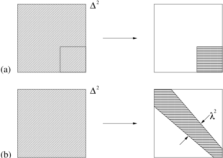
Figure 5: (a) The standard renormalization procedure is based on reduction of a space of states. This leads to small energy denominators in perturbation theory. (b) Similarity renormalization procedure is based on a rotation of basis and avoids small denominators in perturbative derivation of effective dynamics, because it integrates out only these energy changes that are larger than $\lambda$.

The problem is that if there is no finite energy gap in the basis of eigenstates of $H_{0}$ between the retained and integrated out states, then small energy differences between states in the retained subspace and outside of it appear in denominators in perturbative transformation $R$ that is repeatedly used in the renormalization group part of the whole calculation. The small denominators lead to large numbers multiplying terms which depend on $\Delta$, and intruder states can spoil the utility of that procedure completely. Therefore, to cancel the $\Delta$-dependence by the calculated counterterms one would have to make incredibly precise calculations for very large $\Delta$. In the similarity approach, the construction of counterterms and the transformation to small cutoff Hamiltonians are defined quite differently, see Fig. 5b. Instead of integrating states out, one brings the Hamiltonian matrix elements close to the diagonal in the sense that the new interactions change eigenvalues of $H_{0}$ only by less than an arbitrary but finite $\lambda$. The small energy denominators are avoided because one never eliminates transitions with energy changes smaller than $\lambda$, and so the denominators are always bigger than $\lambda$. When one comes to the step of reduction $R$ of $H_{\lambda}$ to a few-body bound-state eigenvalue problem, one already has a well defined effective theory with a small width $\lambda$ and, in principle, no trace of the diverging cutoff parameter $\Delta$.

One more advantage of the similarity approach is that one can also use it to introduce the notion of effective particles Gacta and switch over to the eigenvalue problem written in terms of them, instead of the bare ones. This option allows us to perform practical calculations in QFT in a new way described in the next Section.

V Approach 2: Bound states of two effective fermions

This Section briefly reviews the RGEP for deriving Hamiltonians $H_{\lambda}$ for effective particles of size $\lambda^{-1}$ and then applies $H_{\lambda}$ in the Yukawa theory to a bound state of two effective fermions. The presentation refers to some steps made in the previous Section, but in the context of effective particles instead of the bare ones. Key differences are pointed out, that lead to the two-effective fermion dynamics that converges in the region of large relative momenta.

V.1 Renormalization Group for Effective Particles

The RGEP is defined through a unitary rotation for creation and annihilation operators Gacta

$$b^{\dagger}_{\lambda}=U_{\lambda}b^{\dagger}U^{\dagger}_{\lambda}.$$ (22)

Each operator (such as a Hamiltonian) can be expressed in terms of both sets of the operators: $b$ or $b_{\lambda}$, and it has different matrix elements in the Fock-space basis built using the operators of each kind. The idea of the RGEP is to perform the rotation (22) in such a way, that the Hamiltonian expressed in terms of $b_{\lambda}$, called the “effective Hamiltonian of width $\lambda$”, denoted $H_{\lambda}$, contains vertex form factors $f_{\lambda}$ of width $\lambda$ in all interaction terms. There are infinitely many interaction terms in $H_{\lambda}$ for all finite values of $\lambda$ and their strengths vary with $\lambda$ Ggluon . The choice for $f_{\lambda}$ made here is,

$$f_{\lambda}=\exp\left[-\frac{(M_{created}^{2}-M_{annihilated}^{2})^{2}}{\lambda^{4}}\right]\;,$$ (23)

where $M_{created}$ is a total free mass of all particles created by a given term in $H_{\lambda}$, and $M_{annihilated}$ is a total free mass of particles annihilated by the term.

If the unitary transformation $U_{\lambda}$ were known exactly, there would be no $\lambda$ dependence in the spectrum of $H_{\lambda}$. But when $U_{\lambda}$ (and $H_{\lambda}$) are calculated in perturbation theory, the approximation leads to some residual $\lambda$-dependence of theoretical predictions for observables. The sensitivity of results to variation of $\lambda$, provides a simplest test for how large errors one makes in the perturbative expansion for $H_{\lambda}$, on top of the error margin resulting from approximations used to solve the Schrödinger equation with $H_{\lambda}$. On the one hand, one tries to get down to as small $\lambda$ as possible so that the non-perturbative diagonalization will require smallest possible range of energy scales to handle explicitly, using a computer. On the other hand, one expects errors due to use of perturbation theory in evaluating $H_{\lambda}$ to grow with reducing $\lambda$, and $\lambda$ should not be too small. The reason is that if $\lambda\rightarrow 0$, the Hamiltonian becomes almost diagonal, which is equivalent to solving the non-perturbative dynamics of bound states, and a perturbative calculus for $H_{\lambda}$ must fail at some point before $\lambda$ becomes equal to the scale of the non-perturbative phenomena.

The same rotation $U_{\lambda}$ provides also means for constructing counterterms in $H^{\Delta}=H_{\lambda=\infty}$. A Hamiltonian $H_{\lambda}$ with a finite $\lambda$ has a band diagonal matrix in the effective basis, and each effective Fock basis state is directly coupled only to a limited set of other effective states that have energies within the range of $\lambda$. Therefore, the effective theory splits into a chain of theories that couple only to near neighbors, without jumping up to arbitrarily large scales such as $\Delta$ in the approach 1. Consequently, if counterterms introduced in $H^{\Delta}$ cause that no $\Delta$-dependence appears in the matrix elements of $H_{\lambda}$ in the effective basis states, there can be no $\Delta$-dependence generated in observables calculated in perturbation theory to any finite order when $\Delta/\lambda$ tends to infinity. This will be seen in detail at the end of this Section, but it can be observed already here that the bare-particle approach described in the previous Section did not have this property and $\Delta$-dependence could show up in the bound-state dynamics even though matrix elements of the Hamiltonian reduced to the two-body sector did not depend on $\Delta$ for all finite relative momenta.

V.1.1 Effective Hamiltonian - 0th and 1st order

The only change in the 0th-order Hamiltonian (free part, order $g^{0}$) is that the bare operators such as $b^{\dagger}b$ are replaced by $b^{\dagger}_{\lambda}b_{\lambda}$. In order $g^{1}$, the effective Hamiltonian has the form,

$$H_{\lambda}^{\Delta(1)} = g\sum_{i=1}^{2}\sum_{\sigma_{1},\sigma_{2}}\int\left[p_{1}p_{2}q\right]2(2\pi)^{3}\delta^{3}\left(p_{1}-p_{2}-q\right)\exp\left(-\kappa^{\perp 2}_{p_{2},q}/\Delta^{2}\right)r_{\delta}(x_{q}/x_{p_{1}})\exp\left[-\frac{\left(M_{p_{2}q}^{2}-m^{2}\right)^{2}}{\lambda^{4}}\right]$$ (24)

$$\times\left[a^{\dagger}_{q\lambda}b^{(i)\dagger}_{p_{2}\sigma_{2}\lambda}b^{(i)}_{p_{1}\sigma_{1}\lambda}\bar{u}_{p_{2}\sigma_{2}}u_{p_{1}\sigma_{1}}-a^{\dagger}_{q\lambda}d^{(i)\dagger}_{p_{2}\sigma_{2}\lambda}d^{(i)}_{p_{1}\sigma_{1}\lambda}\bar{v}_{p_{1}\sigma_{1}}v_{p_{2}\sigma_{2}}+h.c.\right]\;.$$

Note that expressing $b$’s by $b_{\lambda}$’s induced the form factor $f_{\lambda}$ in $H_{\lambda}$. This form factor causes that the regularization factor that depends on $\Delta$ is equivalent to 1 when $\Delta/\lambda\rightarrow\infty$.

V.1.2 Effective Hamiltonian - 2nd order: mass term

One can calculate the term in $H_{\lambda}$ of order $g^{2}$ that contains $b_{\lambda}^{\dagger}b_{\lambda}$ and see that it contains a mass-squared-like term with a divergent $\Delta$-dependence. Therefore, one has to add a counterterm to the initial Hamiltonian that has exactly the same form (11) as in the approach 1. After including this counterterm, the form of the effective mass term in $H_{\lambda}$ is (in the limit $\Delta\rightarrow\infty$)

$$H_{\lambda\delta m}=\int[p]b_{\lambda}^{\dagger}b_{\lambda}\frac{\delta m^{2}_{\lambda}}{p^{+}}\;,$$ (25)

where

$$\delta m^{2}_{\lambda} = \frac{g^{2}}{16\pi^{2}}\int_{m^{2}}^{\infty}dz\frac{1}{2}\left(1+\frac{6m^{2}}{z}+\frac{m^{4}}{z^{2}}\right)\times$$ (26)

$$\exp\left[-\frac{2(z-m^{2})^{2}}{\lambda^{4}}\right]+const.$$

Note that the renormalization is carried out now at the level of full theory in the whole Fock space, not after reduction to a specific Fock sector. Therefore, for example, there are no sector-dependent mass counterterms. Since the regulators did not violate any kinematical light-front symmetries, the calculated mass term does not depend on particle momentum (i.e. the relativistic form of the dispersion relation does not change, there is only a change of the value of the effective fermion mass).

V.1.3 Effective Hamiltonian - 2nd order: potential term

Second-order terms in $H_{\lambda}$ that contain two creation and two annihilation operators for effective fermions do not contain any dependence on $\Delta$ when $\Delta\rightarrow\infty$, and no counterterms are needed of such form. Therefore, the complete answer for these terms is

$$H_{\lambda b^{\dagger}b^{\dagger}bb}^{\Delta(2)} = \sum_{\sigma_{1}\sigma_{2}\sigma_{3}\sigma_{4}}\int[p_{1}p_{2}p_{3}p_{4}]b^{(1)\dagger}_{p_{1}\lambda}b^{(2)\dagger}_{p_{3}\lambda}b^{(2)}_{p_{4}\lambda}b^{(1)}_{p_{2}\lambda}\;2(2\pi)^{3}\delta^{3}(p_{1}+p_{3}-p_{2}-p_{4})$$ (27)

$$\times v^{(2)}_{\lambda}(p_{1},p_{2},p_{3},p_{4},\sigma_{1},\sigma_{2},\sigma_{3},\sigma_{4})\;,$$

where

$$v^{(2)}_{\lambda}(p_{1},p_{2},p_{3},p_{4},\sigma_{1},\sigma_{2},\sigma_{3},\sigma_{4})=-g^{2}\bar{u}_{1}u_{2}\bar{u}_{3}u_{4}\frac{1}{q^{+}}f_{ac}{\cal F}_{2}(a,b,c)|_{Fig.\ref{fig:2diag}a}+\text{the same}|_{Fig.\ref{fig:2diag}b}\;,$$ (28)

and ${\cal F}_{2}(a,b,c)=[(xba+(1-y)bc)/(ba^{2}+bc^{2})](f_{ba}f_{bc}-1)$, adopting conventions from Ref. Ggluon with $x=p_{1}^{+}/(p_{1}^{+}+p_{3}^{+})$ and $y=p_{2}^{+}/(p_{2}^{+}+p_{4}^{+})$. Despite that Fig. 2 is referred to in order to define notation, just like in approach 1, the potential $v_{\lambda}$ is quite different from the OBE potential of Eq. (15). For example, note the different kind of denominators and the presence of the key formfactors $f_{ac}$.

V.1.4 Effective Hamiltonian - 2nd order: other terms

In the second-order effective interaction, there are also other terms, similar to the terms shown above, or describing interactions with explicit participation of bosons. There are also terms creating or annihilating two additional particles. None of these terms contribute to the second-order effective equation that will be obtained in the following Section in the case of bound states of two effective fermions. In general, the RGEP allows one to construct both the transformation $U_{\lambda}$ and Hamiltonian $H_{\lambda}$ in perturbation theory to an arbitrary order in $g$. Calculating higher-order corrections is ultimately the only way for finding out how large corrections they produce. The approach 2 is limited here to terms of the second order, because it was the case in the approach 1.

V.2 Solving eigenvalue problem with $H_{\lambda}$

In the case of bound states of two effective fermions, the reduction procedure is based on the same rules as in the approach 1, except that the effective particles interact with vertex form factors of width $\lambda$ and the large relative-momentum convergence is improved. Also the change of particle number is severely limited in strength, since massive particles cease to be produced when $\lambda$ is lowered below their mass, and the emission of massless particles changes energies by amounts linear in the exchanged momentum. The changes of order $k$ are larger than the changes of order $k\times k/m$ in the fermions’ energies when $\lambda$ is smaller than $m$. The departure point of the process of solving the bound state dynamics is the eigenvalue equation for the single fermion states.

V.2.1 Reduction to one effective fermion subspace

This step produces an equation $H_{R}|k\rangle=P^{-}|k\rangle$, where

$$P^{-}=\frac{k^{\perp 2}+m^{2}_{f}}{k^{+}}\;,$$ (29)

and $m^{2}_{f}$ is the physical fermion mass, by definition of the same value as in the approach 1. It comes out independent of $\Delta$ by the virtue of adjusting once and for all the mass squared counterterm in $H^{\Delta}$. The same adjustment involves fixing the free finite constant in Eq. (26) so that for some value of $\lambda=\lambda_{0}$ the physical fermion mass eigenvalue $m_{f}$ equals to the experimentally found number. The interesting point is that the same eigenvalue is subsequently automatically obtained for all values of $\lambda$ and the physical dispersion relation satisfies all requirements of special relativity. This is the simplest manifestation of the general rule that physical results should be independent of $\lambda$, as it is only a parameter of a unitary rotation of the basis.

V.2.2 Reduction to two-effective fermions

Using transformation $R$ to reduce $H_{\lambda}$ to the two-effective particle subspace without restrictions on the relative momenta, one obtains a quantum mechanical interaction that can change the invariant mass of the two particles by a certain $\Lambda$ if, and only if the interaction acts more than $\Lambda/\lambda$ times. Thus, the approach 2 produces an effective Hamiltonian which is free from the overlapping divergence problem discussed in Ref.overlap , and in the previous Section in approach 1. However, in order to make a connection with the non-relativistic two-particle Schrödinger quantum mechanics, which was not systematically available in the approach 1, one needs now to limit the relative momenta in the effective two-particle Fock sector to $k<z$, where $z$ is a new parameter required for defining the new operation $R$ that enables one to define the procedure of introducing the non-relativistic limit.

Therefore, a new transformation $R$ is now defined to lead to a model Hamiltonian $H_{R}$ that acts only in the subspace of the two-effective particles Fock sector with limited invariant masses (Fig. 6). Thus, not only the number of effective particles is limited, but also the range of their relative momenta. It is required that $H_{R}$ has the same spectrum of low lying energy levels as $H_{\lambda}$ has in the whole space. This step is no longer related in any way with infinite renormalization problem as in the approach 1. The existence of such reduction is plausible only because $H_{\lambda}$ has a small width $\lambda$ and in subsequent orders of perturbation theory in $H_{I\lambda}$, corrections to the effective potential result from the coupling to an additional region of relative momenta, which is always limited by $\lambda$ in every new order.

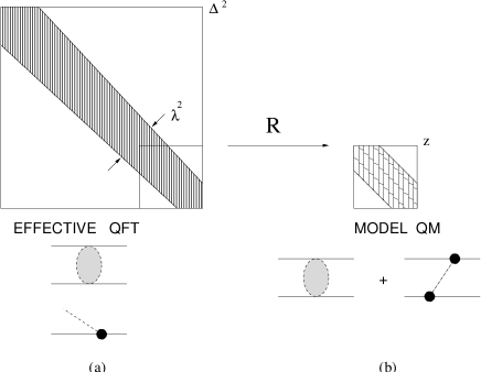
Figure 6: Reduction of effective QFT, (a), to relativistic quantum mechanics in a model subspace, (b), is possible in the approach 2 thanks to the form factors in the effective interaction vertices.

The projection operator used here is

$$\hat{P}=\sum_{\sigma_{1}\sigma_{2}}\int[p_{1}p_{2}]b_{1\lambda}^{(1)\dagger}b_{2\lambda}^{(2)\dagger}|0\rangle\langle 0|b_{2\lambda}^{(2)}b_{1\lambda}^{(1)}\theta\left(z-|\vec{k}|\right)\;,$$ (30)

where $\vec{k}$ is the relative momentum of effective particles of momenta $p_{1}$ and $p_{2}$. Although introduction of $z$ is useful from the conceptual point of view, the formfactors $f_{\lambda}$ imply that $z$ is not important in practice if only the lowest order (i.e. $g^{2}$) model Hamiltonian is calculated (see Fig. 6). I would, however, affect the model Hamiltonian in order $g^{4}$ through terms such as the last two terms in Eq. (36).

The effective Schrödinger equation has then the form of Eq. (14) with $v_{OBE}$ replaced by a new potential, denoted $v_{R\lambda}$, which is a sum of two terms (Fig. 6b). The first term is the projection of $H_{\lambda b^{\dagger}b^{\dagger}bb}^{\Delta(2)}$, cf. Eq. (27), on the two-body space restricted by $z$. The second term comes from the one-effective boson exchange (OEBE) and has a form similar to (15),

$$v_{OEBE\lambda}(\sigma_{1}\sigma_{2}\sigma_{3}\sigma_{4}\vec{k}\vec{k}^{\prime})=-\frac{\pi\alpha}{2m^{2}}{{f_{\lambda}}}\bar{u}_{1}u_{2}{{f_{\lambda}}}\bar{u}_{3}u_{4}\frac{1}{q^{+}}\left(\frac{p^{+}_{ba}}{ba}+\frac{p^{+}_{bc}}{bc}\right)_{Fig.\ref{fig:2diag}a}+\text{the same}|_{Fig.\ref{fig:2diag}b}\;,$$ (31)

except for the form factors $f_{\lambda}$ in vertices and the overall limitation of the momenta by $z$ [not indicated explicitly in Eq (31)]. Each of these two terms (i.e. projection of $H_{\lambda b^{\dagger}b^{\dagger}bb}^{\Delta(2)}$ and $v_{OEBE}$) behave for $k,k^{\prime}\ll m$ like the Coulomb potential (17) with form factors $f_{\lambda}$ that limit changes of the fermion kinetic energies.

Figure 7: First-order correction to the ground state binding energy as a function of $\lambda$ for $z=\infty$, which shows the magnitude of corrections to the well known Schrödinger equation with a Coulomb potential expected in the approach 2 in QFT.

One can approximate the Schrödinger equation with this QFT potential by the equation with a Coulomb potential plus a correction, and one can estimate the size of the correction using bound-state perturbation theory. For this purpose, the difference between potentials $v_{R\lambda}$ and $v_{Coulomb}$ is denoted by $\Delta v_{\lambda}$. The first-order correction, $\Delta E^{(1)}_{\lambda}=\langle\phi_{0}|\Delta v_{\lambda}|\phi_{0}\rangle$, is a function of the parameters $\lambda$ and $z$. Numerical calculation confirms that for $z>\lambda$ there is no noticeable $z$-dependence of this matrix element. Fig. 7 shows how the matrix element depends on $\lambda$ for $z=\infty$. As expected in Section V.1 for small $\lambda$, there is some $\lambda$-dependence in the result. It emerges because at too small $\lambda$s the similarity factors $f_{\lambda}$ start to limit the Hamiltonian in the momentum region that is important for the bound state formation, and the derivation of $H_{\lambda}$ cannot be carried out precisely using the perturbative renormalization group procedure down to so small $\lambda$s. When $\lambda$ and $z$ are large enough, the correction $\Delta E^{(1)}_{\lambda}$ approaches a fixed finite value, that depends on $\alpha$. This happens because the wave function $\phi_{0}$ has a width $a=\alpha\mu$ and limits the integration over both momenta in the matrix element $\langle\phi_{0}|\Delta v_{\lambda}|\phi_{0}\rangle$. Thus, as seen already in Section IV.2, the first-order correction is small for small coupling constants due to the fast fall-off of the Coulomb wave function at large momenta, independently of the details of $\Delta v$ that one obtains in the approaches 1 or 2. The correction is small even for a divergent potential such as a $\delta$-function.

Therefore, one needs to look at the second order of the bound-state perturbation theory to check the self-consistency of the effective particle picture and to compare it to the approach 1. To see that the effective theory does not exhibit the consistency problems the approach 1 exhibited in Fig. 4, one can closely follow here the derivation of Eq. (20), but with the OBE potential $v_{OBE}$ replaced by $v_{R\lambda}$. Again, one can ask whether there is a logarithmically divergent dependence on $k_{max}$.

It turns out that for finite values of $\lambda$ there is no such divergent dependence. One can safely take the limit $k_{max}\rightarrow\infty$, since $\lambda$ itself already cuts off sums over intermediate states in the correction.

$$-\Delta\tilde{E}_{\lambda}^{(2)}=m^{2}\int_{0}^{4\alpha m}\frac{d^{3}k_{1}}{\sqrt{E_{1}}}\int_{m}^{\infty}\frac{d^{3}k_{2}}{E_{2}}\int_{0}^{4\alpha m}\frac{d^{3}k_{3}}{\sqrt{E_{3}}}\phi_{0}(k_{1})\Delta v_{\uparrow\downarrow\lambda}(\vec{k}_{1},\vec{k}_{2})\frac{1}{H_{0}}\Delta v_{\uparrow\downarrow\lambda}(\vec{k}_{2},\vec{k}_{3})\phi_{0}(k_{3})$$ (32)

Here, $\Delta v_{\uparrow\downarrow\lambda}$ is defined similarly to $\Delta v_{\uparrow\downarrow}$, but with $v_{OBE}$ replaced by $v_{R\lambda}$. Numerical results for this matrix element for different values of $\lambda$ (and for the cutoffs $k_{max}\sim\Delta\rightarrow\infty$), are shown in Fig. 8.

Figure 8: Dependence of the large-relative momentum contribution to the second order bound-state mass correction on $\lambda$, for the cutoff $\Delta$ sent to $\infty$. When one works with effective fermions, cutoffs can be sent to $\infty$ for any given value of $\lambda$, which is not available in the approach 1 for bare fermions, as shown in Fig.4.

First of all, the results in Fig. 8 can be considered a good approximation to the whole 2nd-order correction only for $\lambda\gg m$ (i.e. in the right part of the figure). If $\lambda$ is comparable to $m$, the similarity factors $f_{\lambda}$ limit the potential $v_{R\lambda}$ and the high-low and low-high corners of the potential matrix (Fig. 3) are practically eliminated. The correction coming from the large momentum region selected in the integration in Eq. (32) is therefore also reduced and the other of the $2^{4}$ parts of the whole correction can contribute in more significant ways than they do for large $\lambda$. Hence, for small $\lambda$, the results given in Fig. 8 are not necessarily a good approximation of the whole second-order energy-correction.

Secondly, in practical work, one needs to lower $\lambda$ as far down as possible, possibly below $m$. Thus, Fig. 8 provides only evidence for the self-consistency of the effective fermion dynamics in which the convergence in the large-relative momentum region is secured by the presence of $\lambda$, and the original QFT cutoffs can be safely sent to infinity.

Thirdly, despite the reservations made above, one can expect that the exact 2nd-order correction from the large momentum region to the bound-state mass is of the same order of magnitude as the part given in Fig. 8. It is clear then that the 2nd-order contribution from the large-relative momentum range is at least one order of magnitude smaller than the 1st-order result, presented in Fig. 7. Therefore, it is the small and moderate momentum region that decides about the size of variations of observables versus $\lambda$. In view of these three comments the following farther remarks can be made.

It is visible in Fig. 7 in the case of $\alpha=0.01$ that the bound state energy is a very slowly varying function of $\lambda$ when the latter grows above $0.2m_{f}$. One could call this value of $\alpha$ a non-relativistic coupling, because all the important dynamics happens among virtual effective particles with momenta much smaller than the fermion mass. Consequently, if the form factor $f_{\lambda}$ is wider than $0.2m_{f}$, its presence is hardly seen in the final result. Nevertheless, its presence remains to be essential for keeping the 2nd-order correction finite and making the large-momentum region of QFT a small correction (Fig. 8) to the Schrödinger picture when $\Delta\rightarrow\infty$, instead of diverging and invalidating that picture, as it was happening in the approach 1 (Fig. 4). The system of effective particles is then shown to be self-consistently non-relativistic and the Schrödinger equation with Coulomb potential is a good approximation of QFT. Qualitatively, this is the situation encountered in QED with $\alpha=1/137$.

However, as $\alpha$ increases, one has to make $\lambda$ larger to achieve a fair $\lambda$-independence of the total binding energy, by reducing the size of the $\lambda$-dependent corrections. Fig. 7 shows that the first-order corrections can be quite large and they depend on $\lambda$. For $\alpha=0.1$, the correction has a non-negligible value ($\Delta E^{(1)}=0.06E_{0}$) even for $\lambda=m_{f}$. For $\alpha=0.3$ and $\lambda=m_{f}$, $\Delta E^{(1)}=0.12E_{0}$. And if one wanted to make a reduction of the theory to the two-fermion state for $\alpha=0.6$, one would have to include momenta much larger than the fermion mass (for $\lambda=m_{f}$, $\Delta E^{(1)}=0.43E_{0}$, and it still strongly depends on $\lambda$). In this case, the QFT effective two-body equation is no longer close to the non-relativistic Schrödinger equation with the Coulomb potential. Also, strong $\lambda$-dependence suggests that considerable errors can come from the limitation to only second-order perturbative calculation of the similarity rotation. Besides, one should investigate whether perturbation theory for inclusion of higher effective Fock sectors is acceptable when solving the Schrödinger equation.

Fortunately, as one can see from Fig. 8, at the same time the second-order corrections coming from large momenta remain small, even for $\alpha=0.6$. This is an important result, because it suggests that preparing numerical procedures for solving effective particle dynamics with a few Fock sectors and seeking better starting points for the bound-state perturbation theory than the pure Coulomb picture, is a good idea to try. Namely, if the region of large relative momenta were significant (and not manageable in perturbation theory, contributing too much in the second order), there would be no reason for why limiting the number of Fock sectors should be a legitimate approximation. The uncertainty principle would rather suggest that if momenta larger than $m_{f}$ are important then multiparticle states are also important. Our result says, that thanks to $f_{\lambda}$ one can expect the effective Fock space expansion to be a legitimate strategy in the approach 2, although it requires checking.

Finally, the difference between the initial cutoff $\Delta$ and the parameter $\lambda$ is important for a self-consistent interpretation of the theory. The cutoff $\Delta$ is an artificial parameter that chops off the high-energy part of the initial QFT Hamiltonian. One wants to send $\Delta$ to infinity and one chooses counterterms in $H^{\Delta}$ in such a way that observables are independent of $\Delta$ in the limit $\Delta\rightarrow\infty$. The same huge cutoff appears in the Tamm-Dancoff procedure with bare particles. There is then no alternative in the approach 1 to sending $\Delta$ to infinity in the reduction to two-bare fermions Fock sector. This is odd because there is no good reason for only a few bare particles to be relevant in the bound-state dynamics with the huge momentum cutoff. Indeed, new overlapping divergences are obtained this way. Without tools to handle the problem, no self-consistent relativistic treatment of bound states of fermionic constituents in QFT can be reached that way (see also Section IV.1).

In the conceptually different approach 2, $\Delta$ is absent in the effective particle dynamics, and the new finite width parameter $\lambda$ is introduced. One adjusts $\lambda$ to contain the actual physics of the theory in most economic way, and the key measure of success in this respect, besides verifying symmetries, is provided by the size of changes in the physical results when $\lambda$ is changed. Comparing the first and second-order results from Figs. 7 and 8, one can see that there is a whole range of $\lambda$s and coupling constants of considerable interest where stability of results versus $\lambda$ can be expected in more advanced calculations than used in the present pilot study. The renormalization group flow of $H_{\lambda}$ produces important corrections to the well known non-relativistic picture, visible in the significant first-order corrections, while the large-relative momentum region is self-consistently protected from divergences. This way, a relativistic treatment of bound states of fermions in the Fock space has a chance to be developed poincare .

VI Conclusions

One can attempt to calculate wave functions of bound states of fermions in the Fock space representation of the Yukawa QFT in various ways that are described and compared in the previous Sections on the example of bound states of two fermions. Two basic concepts are distinguished. One approach starts from the sector of two bare fermions (approach 1), and another one from two effective fermions (approach 2).

Approach 1 leads to overlapping divergences in the light-front Hamiltonian dynamics and lacks self-consistency in handling the large-relative momentum region when one attempts to send the bare cutoff to infinity without including infinitely many bare particles. There exists an option of removing this defect through sector dependent counterterms, but the required construction of the full renormalization group triangle with growing numbers of bare particles appears overwhelmingly complex and certainly not completely understood. The basic ultraviolet problem comes from short distances in the transverse directions and no practical tool exists yet for handling huge numbers of bare particles with precision required by rotational, parity, and other symmetries of the initial Lagrangian.

Approach 2 is free from the difficulties with large-relative momentum convergence of the approach 1. The decisive convergence factor is introduced through solving renormalization group equations for effective particles. The solution includes form factors of width $\lambda$ in the interaction vertices and the form factors suppress the large momentum domain. This is verified in numerical estimates described in previous Sections. The well-known one-boson-exchange (OBE) potentials that are deduced from the on-shell $S$-matrix elements, are replaced by new one-effective-boson-exchange (OEBE) potentials, and additional interactions, that are derived in the Hamiltonian form independently of the corresponding $S$-matrix. Moreover, one can take advantage of subsequent $S$-matrix calculation in choosing free finite parts of the counterterms. Then the renormalized Hamiltonians in the QFT Fock space, include relativistic and off-energy-shell corrections in accordance with first principles of quantum mechanics, special relativity, and renormalization group. However, these principles are satisfied only approximately, since the solutions for $H_{\lambda}$ are found only order by order in perturbation theory, and diagonalization of the reduced Hamiltonians $H_{R}$ is carried out numerically. The approximate character is not a weakness, however, because corrections can be systematically investigated and reduced.

The accuracy of the approximate treatment can be estimated by inspecting variation of results when one changes the renormalization group parameter $\lambda$. Exact theory would exhibit no dependence on $\lambda$. In the approximate treatment, variations depend on the size of the coupling constants.

For $\alpha$ smaller than about 0.3, there is a wide range of $\lambda$s in the Yukawa theory with massless bosons, in which the results for the two-fermion bound state mass are stable and do not differ much from results obtained from the nonrelativistic Schrödinger equation with Coulomb potential. These values of $\alpha$ can be called non-relativistic. For $\alpha$ larger than about 0.3, one has to allow $\lambda$ to grow up to the size on the order of $m_{f}$, to achieve $\lambda$-independence of the corrections to the bound-state mass. This means that relativistic momenta do matter and the non-relativistic Schrödinger equation is not a good approximation of the effective dynamics. Still, the effective theory is well contained in the range determined by $\lambda$ and one can look for solutions of the eigenvalue problem without making non-relativistic approximation. For the first-order bound-state perturbation-theory corrections to the non-relativistic approximation are quite considerable, while the large-relative momentum region in second-order corrections contributes merely about 10%. Being limited by $\lambda$, it does not introduce any diverging contributions and one does not and should not attempt sending $\lambda$ to infinity, in contrast to the cutoff $\Delta\rightarrow\infty$ in the approach 1.

All effective-particle calculations are carried out here in the light-front form of Hamiltonian dynamics, preserving its kinematical covariance under boosts. This form enables one to separate the relativistic motion of bound states from their internal constituent dynamics. Thanks to this separation, one can reduce the description of the binding mechanism to the Schrödinger equation for internal motion of the constituents without choosing a specific frame of reference. All eigenvalue equations derived here are independent of the total momentum of the states they describe. Thus, the boost symmetry allows one to understand moving bound states in arbitrary motion as soon as one understands them at rest, which can help in understanding their structure in the infinite momentum frame, the opportunity not available in the standard form of Hamiltonian dynamics. In fact, the effective particle dynamics is in principle well-prepared to tackle Poincaré symmetry issues in the Fock space including both the kinematical and dynamical transformations poincare .

When the effective light-front theory is defined in a perturbative way, the vacuum structure remains simple, i.e. $b_{\lambda}|0\rangle=d_{\lambda}|0\rangle=a_{\lambda}|0\rangle=0$. In the calculations reported in this paper, in Yukawa theory, no vacuum structure appeared. In the case of theories where spontaneous symmetry breaking may occur, one has to include new terms in the initial Hamiltonian that contain the information about the possibility that some symmetry may be broken spontaneously KWetal . No such terms were introduced here.

It is certainly possible to apply the reduction scheme described here to other theories than Yukawa. Especially interesting case would be QCD, reduced to a nonrelativistic Schrödinger equation for bound states of constituent quarks, since such physical picture is the basis of phenomenology of hadrons in the particle data tables. It is not precisely clear how such picture could follow from the canonical QCD itself in any other approach. The fact found here that in the Yukawa theory one could enhance the coupling constant even up to 0.3 or 0.6 and the constituent picture remained convergent in the large-relative momentum region, is encouraging, because in QCD one expects the running coupling to be on the order of 1 for widths approaching 1 GeV, cf. GWafbs ; Ggluon .

The discussion of bound states of effective fermions would not be complete without answering the question of how the binding of effective particles such as nucleons might emerge from a theory such as QCD. When the latter is already written in terms of effective quarks and gluons with small $\lambda$, the Hamiltonian matrix in the effective-particle basis can be cut into block pieces that lie along the diagonal, and touch each other with their corners (see Fig. 9), some matrix elements being left out.

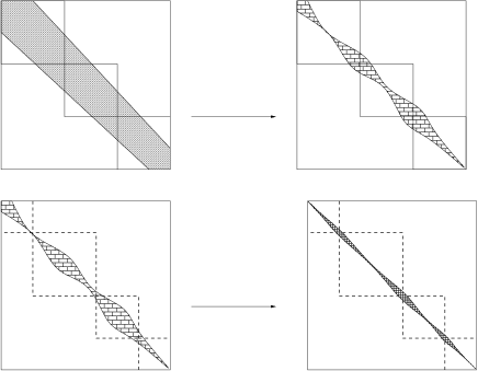
Figure 9: Qualitative representation of the idea of solving the band diagonal problem in effective Fock state basis in a sequence of diagonalizations of “small” matrices. The width of the shaded areas qualitatively represents energy range of the couplings between basis states obtained from a new diagonalization step.

Each of the small blocks can be treated as a separate theory and solved. As a result, one obtains eigenstates or scattering states which are closest to true solutions when their energies lie somewhere in the middle of a block. The accuracy of the solutions diminishes towards the corners where the small triangle parts should provide increasingly important perturbations from couplings to the neighboring blocks. Fig. 9 is drawn in the basis of effective quarks and gluons. Baryons and mesons in QCD would correspond to the approximate solutions in the individual blocks. It is natural to call the blocks channels and the calculation including the interactions between the blocks a coupled-channel theory. The transition from the original degrees of freedom (here, effective quarks and gluons) to the reduced degrees of freedom (baryons and mesons) is achieved by choosing the new basis of states: those given by the solution to the channels dynamics when they are treated as separate. Thus, the lowest mass channel with baryon number 2 contains only nucleons interacting through potentials, the next channel with invariant masses between $2m_{N}+m_{\pi}$ and $2m_{N}+2m_{\pi}$ may include two nucleons and one pion, etc. The bound or scattering states from higher blocks could be approximated by products of the eigenstates from lower-mass blocks. From the mathematical point of view, the transition step is a change of basis in describing eigenstates of relatively small matrices (in comparison to the initial Hamiltonian matrix) and taking into account the residual interactions between different channels later to refine the basis states. The refinement step would be executed in the new basis using the same type of division into blocks, but with the new blocks centered where the previous blocks were least accurate. This sequence of steps can be repeated many times. Thus, the whole transition process to the effective theory written in terms of new degrees of freedom would form a sequence of patterns indicated in Fig. 9. The shaded shapes in Fig. 9 indicate the boundaries of non-zero matrix elements of the effective Hamiltonian matrices between the incoming and outgoing states, which qualitatively indicates their range in energy.

By the way, it is also natural to see in similar terms the transition from electrons and nuclei to atoms, or from atoms to molecules. The universal character of this scheme is the change of basis in the Hilbert space of states in quantum mechanics, and the Hamiltonian scheme for effective particles does open this option to detailed studies in all these theories. Once the width is sufficiently small, it slows down, or freezes degrees of freedom that require larger mass changes than $\lambda$ to be excited. One can also imagine that reducing the width farther in the new basis, a next level of effective degrees of freedom can be isolated using the same scheme. If the reduction were started with a theory underlying QCD, i.e. at extremely large $\lambda$, the scope of the reduction scheme would be even greater.

As a final remark let us indicate that quantum field theories such as Yukawa theory, or sigma-models, may be helpful in discovering the acceptable structure of channel Hamiltonians even without making the transition from QCD to nucleons and mesons explicitly. This option follows from the fact that when the width in the effective theory is made small enough, the meson-fermion vertex contains a narrow form factor and the emission of mesons is weak and slow, even for quite large coupling constants. The structure of the small-width effective theory may be then rather simple and universal in the sense that many initial complex theories may reduce to the same small-width effective one. Thus, the apparently academic Yukawa theory, or other QFTs of that kind, may become very useful in indicating what kind of effective reduced Hamiltonians one can expect from the more elaborate analysis that derives nucleon-pion dynamics from QCD. In fact, a small number of free parameters, such as the form factor width, the size of the coupling constant, or the size of effective masses in a basic set of terms, may be sufficient to reproduce the bulk of the effective model predictions. It is also possible that no significant width dependence is observed in the model results if the parameters are correlated as if the effective model were derived from a Yukawa theory or a sigma-model using only a perturbative expansion for artificially small couplings that only later are extrapolated to the required large values BGP ; TM .

Appendix A Reduction procedure

The eigenvalue equation for a Hamiltonian $H$,

$$H|\psi\rangle=E|\psi\rangle\;$$ (33)

for some low eigenvalues, is replaced using the operation $R$ Bloch ; Wold by an eigenvalue equation for eigenstates $|\varphi\rangle=\sqrt{\hat{P}+R^{\dagger}R}|\psi\rangle$ of the reduced Hamiltonian $H_{R}$, given by the following formula,

$$H_{R}=\frac{1}{\sqrt{1+R^{\dagger}R}}({\hat{P}}+R^{\dagger})H({\hat{P}}+R)\frac{1}{\sqrt{1+R^{\dagger}R}}\;.$$ (34)

If one splits the initial Hamiltonian into the free and interaction parts,

$$H=H_{0}+H_{I}\;,$$ (35)

one can look for $R$ and $H_{R}$ in perturbation theory in $H_{I}$. This leads to the lowest (second order) expression for $H_{R}$:

$$H_{R}={\hat{P}}H{\hat{P}}+\frac{1}{2}{\hat{P}}H_{I}{\hat{Q}}\underline{H_{I}}{\hat{P}}-\frac{1}{2}{\hat{P}}\underline{H_{I}}{\hat{Q}}H_{I}{\hat{P}}+\dots$$ (36)

where the underlining denotes free energy denominators, displayed in Eq.(4).

Appendix B Notation for spinors

The four-component spinors of fermions and anti-fermions in light-front Hamiltonians have the following form.

$$u_{mp\lambda} = \frac{1}{\sqrt{mp^{+}}}\left[p^{+}\Lambda_{+}+\Lambda_{-}(m+\alpha^{\perp}p^{\perp})\right]u_{\lambda}\;,$$

$$v_{mp\lambda} = \frac{1}{\sqrt{mp^{+}}}\left[p^{+}\Lambda_{+}+\Lambda_{-}(m+\alpha^{\perp}p^{\perp})\right]v_{\lambda}\;,$$ (37)

where the projection operators are given by

$$\Lambda_{\pm}=\frac{1}{2}\gamma^{0}\left(\gamma^{0}\pm\gamma^{3}\right)=\frac{1}{2}\gamma^{0}\gamma^{\pm}\;,$$ (38)

the spinors of particles of zero velocity equal

$$\begin{array}[]{rclccrcl}u_{\uparrow}&=&\sqrt{2m}\left(\begin{array}[]{c}\chi_{1}\\ 0\end{array}\right)&,&u_{\downarrow}&=&\sqrt{2m}\left(\begin{array}[]{c}\chi_{-1}\\ 0\end{array}\right)\;,\\ v_{\uparrow}&=&\sqrt{2m}\left(\begin{array}[]{c}0\\ \chi_{-1}\end{array}\right)&,&v_{\downarrow}&=&\sqrt{2m}\left(\begin{array}[]{c}0\\ -\chi_{1}\end{array}\right)\;,\end{array}$$ (39)

and the two-component spinors are

$$\chi_{1}=\left(\begin{array}[]{c}1\\ 0\end{array}\right)\quad\quad,\quad\quad\chi_{-1}=\left(\begin{array}[]{c}0\\ 1\end{array}\right)\;.$$ (40)

The matrices appearing on the right hand side of Eq. (37) represent Lorentz transformations belonging to the small group that preserves the four-vector $\eta$ defining the light front $x^{+}=0$ through the condition $\eta x=x^{+}$, where $x$ is an arbitrary four-vector.

Fermion field operator fulfilling free Euler-Lagrange equations $\psi_{m}(x)$ is expanded for light-front “time” $x^{+}=0$ in terms of creation and annihilation operators as:

$$\psi_{m}^{(i)}(x)|_{x^{+}=0}=$$

$$=\sum_{\sigma}\int[p]\left[b_{p\sigma}^{(i)}u_{mp\sigma}e^{-ip_{\mu}x^{\mu}}+d_{p\sigma}^{(i)\dagger}v_{mp\sigma}e^{ip_{\mu}x^{\mu}}\right]\;.~{}~{}~{}~{}~{}~{}~{}$$ (41)

Appendix C Light-front momenta

For two particles of momenta $p_{1}$ and $p_{2}$, the total momentum $P$ and the relative momenta $x$, $\kappa^{\perp}$ are defined as follows.

$$p_{1}^{+} = xP^{+}\;,$$ (42)

$$p_{2}^{+} = (1-x)P^{+}\;,$$ (43)

$$p_{1}^{\perp} = xP^{\perp}+\kappa^{\perp}\;,$$ (44)

$$p_{2}^{\perp} = (1-x)P^{\perp}-\kappa^{\perp}\;.$$ (45)

Unless stated otherwise,

$$\delta^{3}(k-p)=\delta^{2}(k^{\perp}-p^{\perp})\delta(k^{+}-p^{+})\;.$$ (46)

The shorthand notation in the integrals involves the measure

$$[p]=\frac{d^{2}p^{\perp}dp^{+}}{2(2\pi)^{3}p^{+}}\;.$$ (47)

Creation and annihilation operators are normalized by the commutation relation

$$\left[a_{p},a_{k}^{\dagger}\right]=2(2\pi)^{3}k^{+}\delta^{3}(k-p)\;$$ (48)

for bosons, and in analogous way by anticommutation relations for each kind of fermions.

In order to exhibit relationship between QFT and the well-known equal-time Schrödinger equation, one uses relative momentum $\vec{k}$ jmn ,

$$k^{\perp} = \kappa^{\perp}$$ (49)

$$k_{3} = \sqrt{\frac{\kappa^{\perp 2}+m^{2}}{x(1-x)}}\left(x-\frac{1}{2}\right)\;,$$ (50)

or, equivalently,

$$x=\frac{1}{2}\left(1+\frac{k_{3}}{\sqrt{\vec{k}^{2}+m^{2}}}\right)\;.$$ (51)

Appendix D Schrödinger’s solution in Coulomb potential

Equation

$$\frac{\vec{k}^{2}}{2\mu}\phi(\vec{k})-\int\frac{d^{3}k^{\prime}}{(2\pi)^{3}}\frac{4\pi\alpha}{(\vec{k}-\vec{k}^{\prime})^{2}}\phi(\vec{k}^{\prime})=-B\phi(\vec{k})$$ (52)

(the Schrödinger equation for positronium without spin and with reduced mass $\mu=m/2$) has the ground state eigenvalue

$$B_{0}=\frac{1}{2}\mu\alpha^{2}\;,$$ (53)

and the normalized ground state wave function

$$\phi_{0}(k)=N\frac{1}{(a^{2}+k^{2})^{2}}\;,$$ (54)

with $N=\sqrt{8\alpha^{5}\mu^{5}}/\pi$ and $a=\alpha\mu$.

References

- (1) K. G. Wilson, Phys. Rev. D 10, 2445 (1974); see also K. G. Wilson, in C76-01-19.14 CLNS-327, presented at Coral Gables Conf., Miami, Fla, Jan 19-22, 1976; and references therein.
- (2) M. A. Schifman, A. I. Vainstein, V. I. Zakharov, Nucl. Phys. B 147, 385 (1979); and references therein.
- (3) S. D. Głazek and K. G. Wilson, Phys. Rev. D 48, 5863 (1993).
- (4) K. G. Wilson, et al., Phys. Rev. D 49, 6720 (1994); and references therein.
- (5) S. D. Głazek, Acta Phys. Polon. B 29, 1979 (1998); ibid. 31, 909 (2000).
- (6) S. D. Głazek and K. G. Wilson, Phys. Rev. D 57, 3558 (1998).
- (7) F. Wegner, Ann. Phys. (Leipzig) 3, 77 (1994).
- (8) S. D. Głazek, Phys. Rev. D 63, 116006 (2001).
- (9) S. D. Głazek, T. Masłowski, Phys. Rev. D 65, 065011 (2002).
- (10) F. J. Wegner, Phys. Rep. 348, 77 (2001).
- (11) R. J. Perry, Phys. Rep. 348, 33 (2001); and references therein.
- (12) I. Tamm, J. Phys. (USSR)9, 449 (1945).
- (13) S. M. Dancoff, Phys. Rev. 78, 382 (1950).
- (14) S. Głazek, A. Harindranath, S. Pinsky, J. Shigemitsu and K. Wilson, Phys. Rev. D 47, 1599 (1993).
- (15) R. J. Perry, A. Harindranath and K. G. Wilson, Phys. Rev. Lett. 65, 2959 (1990).
- (16) S. J. Brodsky, J. R. Hiller and G. McCartor, Phys. Rev. D 60, 054506 (1999) ; S. J. Brodsky, J. R. Hiller and G. McCartor, Phys. Rev. D 58, 025005 (1998) ; H. C. Pauli, S. J. Brodsky, Phys. Rev. D 32, 2001 (1985).
- (17) A. Casher, Phys. Rev. D14, 452 (1976); C.B. Thorn, Phys. Rev. D20, 1934 (1979); cf. H. C. Pauli, S. J. Brodsky, Phys. Rev. D32, 2001 (1985).
- (18) M. Brisudova and R. J. Perry, Phys. Rev. D 54, 1831 (1996); ibid. D 54, 6453 (1996); M. Brisudova, R. J. Perry, K. G. Wilson, Phys. Rev. Lett. 78, 1227 (1997).
- (19) B. D. Jones, R. J. Perry and S. D. Głazek, Phys. Rev. D 55, 6561 (1997).
- (20) M. Brisudova, Nucl. Phys. Proc. Suppl. 108, 173 (2002); M. Brisudova, Mod. Phys. Lett. A 17, 59 (2002).
- (21) C. Bloch, Nucl. Phys. 6, 329 (1958).
- (22) K. G. Wilson Phys. Rev. D2, 1438 (1970).
- (23) See e.g. K. Bardakci and M. B. Halpern, Phys. Rev. 176, 1686 (1968); L. Susskind, ibid. 165, 1535 (1968); S.-J. Chang, R. G. Root, and T.-M. Yan, ibid. D7, 1133 (1973); S.-J. Chang and T.-M. Yan, ibid., 1147; T.-M. Yan, ibid., 1760, 1780, and references therein.
- (24) S. Głazek, “Weinberg equation with spin”, M. Sc. diploma work, Warsaw University, Institute of Theoretical Physics (1980); see also Acta Phys. Polon. B 15, 889 (1984).
- (25) M. Mangin-Brinet, J. Carbonell and V.A. Karmanov, Phys. Rev. D64:125005 (2001).
- (26) S. D. Głazek and K. G. Wilson, Phys. Rev. D 47, 4657 (1993).
- (27) A. B. Bylev, S. D. Głazek and J. Przeszowski, Phys. Rev. C 53 (1996) 3097.
- (28) T. Masłowski and M. Wiȩckowski, Phys. Rev. D 57, 4976 (1998).
- (29) See e.g. P. Danielewicz and J. M. Namysłowski, Phys. Lett. 81B 110 (1979).