Logarithmic conformal field theory with boundary

Abstract

This lecture note covers topics on boundary conformal field theory, modular transformations and the Verlinde formula, and boundary logarithmic CFT. An introductory review on CFT with boundary and a discussion of its applications to logarithmic cases are given. LCFT at $c=-2$ is mainly discussed.

1 Introduction

Conformal field theories with logarithmic correlation functions have been studied actively for the past several years. Such theories arise naturally as generalisations of the well-investigated unitary Virasoro minimal theories or WZNW theories with integral level, and are believed to have many applications in statistical models and string / brane physics. These logarithmic conformal field theories (LCFTs) were investigated sporadically by several authors[1, 2, 3, 4] in the late eighties and early nineties, and systematic study started with Gurarie’s work[5] in 1993. By now various models, e.g. $c=-2$ model[3, 5, 6, 7], gravitationally dressed CFTs[8, 9], WZNW models with fractional $k$[4, 10] and $k=0$[11, 12, 13, 14] have been studied, and a number of applications, including critical polymers[3, 15, 16], percolation[17, 18], quantum Hall effect[19, 20], disordered systems[11, 12, 21, 22, 23], sandpile model[24], turbulence[25, 26, 27], MHD[28], D-brane recoil[29, 30], etc. have been discussed. Readers are referred to the other lecture notes[31, 32, 33] of the summer school for more complete historical account and description on the state of the art of the study of LCFT.

This article is intended to give an overview of basic concepts in boundary conformal field theory, and to present recent attempts to apply them to logarithmic theories. Motivation for considering boundaries in CFTs is somewhat obvious when we try to model statistical systems: any existing sample of material has finite extent and a theory on the infinite plane is only approximately valid. In order to model the system near the boundary where the finite-size effect is not negligible, we need to define CFT on a topology with boundary. Boundary CFT is also essential for string theory. In the past decade higher-dimensional objects called branes have attracted much attention. Branes are defined as end points of open strings, and are described using boundary CFTs. The study of branes is developing rapidly, and after the emergence of the brane-world scenario, phenomenological interest is growing as well. Apart from these ‘physical’ aspects, boundary CFT is an attractive subject because of its beautiful mathematical structure. It is well known that the modular invariance of partition functions on the torus leads to the classification of rational conformal theories. For the conformal theories with boundary, the modular invariance gives a classification of boundaries which may be realised in a physical system. These modular properties arise from the fact that characters of rational CFTs happen to be linear representation of the modular group.

Boundary logarithmic conformal theory is admittedly rather a young subject, and the known results so far depend on a few simple models. This article presents mainly two topics: the first is on properties of boundary correlation functions[34], and the second is on the classification of boundary states based on modular invariance[35]. We shall discuss these for the $c=-2$ model, after reviewing basic ideas of boundary CFT applied to non-logarithmic examples. These results are based on straightforward generalisation of standard concepts in boundary CFT to the simplest logarithmic theory, and more discussions such as those based on some concrete physical models are desirable. Nevertheless such an attempt is clearly a natural first step to the thorough understanding of logarithmic theories, and we believe these topics are important for the development of non-unitary conformal theories in general.

This article is organised as follows. In the next section we review some basic concepts and techniques in ordinary boundary conformal field theory. In particular, derivation of boundary correlation functions (Subsec.2.2) and Cardy’s classification of boundary states (Subsec.2.3) are given in detail. We also mention Verlinde formula and boundary operators. In Sec. 3 we apply these ideas to $c=-2$ logarithmic theory with boundary, where boundary correlation functions and Cardy’s classification are discussed mainly. We summarise, conclude, and give some prospects in Sec. 4. As the discussion of Sec.3.4 is similar to more familiar Ising model ($c=1/2$) case, we summarise the Majorana fermion construction of the boundary states of the Ising model in App.A. Some formulae on elliptic functions are collected in App.B.

2 Conformal field theory with boundary

In this section we review standard techniques and concepts in non-logarithmic boundary conformal field theory. What we have in mind is simple diagonal unitary minimal models, such as the Ising model. We start, in the first subsection, by discussing conformal invariance in the presence of a boundary. In Subsec.2.2 we review the mirroring method[36] for finding boundary correlation functions. We describe in Subsec.2.3 the classification of consistent boundary states based on the modular invariance, which is known as Cardy’s fusion method[37]. The relation between the modular transformation matrix and the fusion rule (Verlinde formula[38]) and its relevance in the boundary theory[37] is reviewed in Subsec.2.4. In Subsec.2.5 we discuss boundary operators[37, 39] and give an example of a statistical model[17] where the concept of boundary operators plays a central role.

2.1 Conformal transformation with boundary

Let us start by considering what is meant by conformal invariance in the presence of a boundary. Let

$$ds^{2}=g_{\mu\nu}(x)dx^{\mu}dx^{\nu},$$ (1)

be the line element of the manifold we work on. Since the metric is a tensor, it transforms as

$$g^{\mu\nu}(x)\rightarrow\tilde{g}^{\mu\nu}(\tilde{x})=\frac{\partial\tilde{x}^{\mu}}{\partial x^{\lambda}}\frac{\partial\tilde{x}^{\nu}}{\partial x^{\rho}}g^{\lambda\rho}(x).$$ (2)

The conformal transformation is defined as a mapping which preserves the metric $g^{\mu\nu}(x)$ up to a scale factor,

$$g^{\mu\nu}(x)\rightarrow\tilde{g}^{\mu\nu}(\tilde{x})=\Omega(x)^{2}g^{\mu\nu}(x).$$ (3)

In two dimensions this condition is written as

$$\left(\frac{\partial\tilde{x}^{0}}{\partial x^{0}}\right)^{2}+\left(\frac{\partial\tilde{x}^{0}}{\partial x^{1}}\right)^{2}=\left(\frac{\partial\tilde{x}^{1}}{\partial x^{0}}\right)^{2}+\left(\frac{\partial\tilde{x}^{1}}{\partial x^{1}}\right)^{2},$$ (4)

$$\frac{\partial\tilde{x}^{0}}{\partial x^{0}}\frac{\partial\tilde{x}^{1}}{\partial x^{0}}+\frac{\partial\tilde{x}^{0}}{\partial x^{1}}\frac{\partial\tilde{x}^{1}}{\partial x^{1}}=0,$$ (5)

which are equivalent either to

$$\frac{\partial\tilde{x}^{0}}{\partial x^{0}}=\frac{\partial\tilde{x}^{1}}{\partial x^{1}},\;\;\frac{\partial\tilde{x}^{1}}{\partial x^{0}}=-\frac{\partial\tilde{x}^{0}}{\partial x^{1}},$$ (6)

or to

$$\frac{\partial\tilde{x}^{0}}{\partial x^{0}}=-\frac{\partial\tilde{x}^{1}}{\partial x^{1}},\;\;\frac{\partial\tilde{x}^{1}}{\partial x^{0}}=\frac{\partial\tilde{x}^{0}}{\partial x^{1}}.$$ (7)

These are the Cauchy-Riemann equations and their antiholomorphic counterpart. Defining $z=x^{0}+ix^{1}$ and $\bar{z}=x^{0}-ix^{1}$, we conclude that the conformal transformation in two-dimensions (without considering boundary) is equivalent to analytic mapping on the complex plane[40].

On the full plane, the conformal mapping

$$z\rightarrow w(z)=\sum_{n}a_{n}z^{n},$$ (8)

$$\bar{z}\rightarrow\bar{w}(\bar{z})=\sum_{n}\bar{a}_{n}\bar{z}^{n},$$ (9)

is generated by an infinite number of generators $a_{n}$ and $\bar{a}_{n}$, which imposes strict constraints on the field theory. In a geometry with boundary, we may take the line $x^{1}=0$ as the boundary and consider a CFT on the upper half plane. As the field theory is restricted to a fixed geometry, the conformal transformation must keep the boundary $x^{1}=0$ invariant. This means

$$\mbox{Im}\;w(x)|_{x^{1}=0}=0\;\;\Leftrightarrow\;\;w(x^{0})=\bar{w}(x^{0})\;\;\Leftrightarrow\;\;a_{n}=\bar{a}_{n}.$$ (10)

Although the number of generators is reduced by half due to this condition, we still have an infinite dimensional conformal group and conformal invariance remains extremely powerful[41]. Note that the holomorphic and antiholomorphic generators are coupled on the boundary. This allows us to interpret the antiholomorphic part as an analytic continuation of the holomorphic part, as we shall see in the next subsection.

2.2 Boundary correlation functions

The existence of null vectors in minimal CFTs allows us to find $n$-point correlation functions as solutions to differential equations of hypergeometric type[42]. This method was generalised to CFTs on the half plane by Cardy[36], using the mirroring technique which is familiar in electrostatics. In this subsection we review this method and find the spin correlation functions of the Ising model on the upper half plane.

The behaviour of correlation functions under the conformal transformations is described by the conformal Ward identities. For a CFT on the upper half plane they are

$$\delta\langle\phi_{1}\phi_{2}\cdots\rangle\ =\frac{-1}{2\pi i}\oint_{C}dz\epsilon\langle T(z)\phi_{1}\phi_{2}\cdots\rangle+\frac{1}{2\pi i}\oint_{C}d\bar{z}\bar{\epsilon}\langle\bar{T}(\bar{z})\phi_{1}\phi_{2}\cdots\rangle,$$ (11)

as $z\rightarrow w=z+\epsilon$, $\bar{z}\rightarrow\bar{w}=\bar{z}+\bar{\epsilon}$, and $\bar{\epsilon}=\epsilon^{*}$. The contours are the semicircle $C$ which encircles all the coordinates $(z_{i},\bar{z}_{i})$ of the operators (Fig.1a). Since there is no energy-momentum flow across the boundary, the energy-momentum tensor satisfies the condition

$$\left[T-\bar{T}\right]_{z=\bar{z}}=0,$$ (12)

on the boundary $z=\bar{z}$. This condition also means the diffeomorphism invariance of the boundary as the conformal transformation is generated by the energy-momentum tensor. We can use the condition (12) to extend the domain of definition of $T(z)$, by mapping the antiholomorphic part on the upper half plane (UHP) to the holomorphic part on the lower half plane (LHP), as $T(z^{*})=\bar{T}(\bar{z})$. The antiholomorphic dependence of the correlation function on the UHP coordinates is similarly mapped to the holomorphic dependence on the LHP coordinates. The antiholomorphic part of the Ward identities (11) is then mapped into the holomorphic part on the LHP, as shown in Fig.1b. The direction of the integration contour on the LHP is reversed (Fig.1c) by changing the sign of the second term in (11). Since the two contours along the boundary cancel each other, the contours can be concatenated to make contour of full circle (Fig.1d), leading to a much simpler conformal Ward identity,

$$\delta\langle\phi_{1}\phi_{2}\cdots\rangle=\frac{-1}{2\pi i}\oint_{C-C^{*}}dz\epsilon(z)\langle T(z)\phi_{1}(z_{1})\bar{\phi}_{1}(z_{1}^{*})\phi_{2}(z_{2})\bar{\phi}_{2}(z_{2}^{*})\cdots\rangle.$$ (13)

This means that the $n$-point function on the UHP satisfy the same differential equation as the chiral $2n$-point function on the full plane, with the LHP coordinates obtained through mirroring with respect to the boundary.

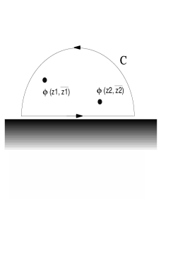
(a) Contour $C$ on UHP.                                (b) Mirroring: $C\rightarrow C^{*}$.
                            
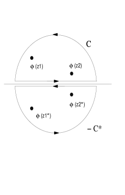
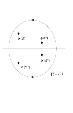
(c) Reverse the direction.                             (d) Merge two contours.

Figure 1: The antiholomorphic coordinate dependence of CFT on the UHP (a) is mapped to the holomorphic dependence on the LHP by mirroring (b). Flipping the direction of the contour on the LHP (c), and merging the two contours, the Ward identity of the $n$-point function on the UHP is shown to be equivalent to that of the $2n$-point function on the full plane.

Let us see this in the example of the Ising model, and find the spin-spin correlation function on the UHP. As the boundary $2$-point function on the half plane is equivalent to the $4$-point function on the full plane, one may write

$$\langle\sigma(z_{1},\bar{z}_{1})\sigma(z_{2},\bar{z}_{2})\rangle_{UHP}=\langle\sigma(z_{1})\sigma(z_{2})\sigma(z_{1}^{*})\sigma(z_{2}^{*})\rangle_{chiral},$$ (14)

where $\sigma$ is the spin operator. Due to the existence of a singular vector at level 2, the $4$-point function of $\sigma=\phi_{1,2}$ satisfies a second order differential equation,

$$\left\{\partial_{z}^{2}-\frac{3}{4}\sum_{i=1}^{3}\left[\frac{1}{z-z_{i}}\partial_{z_{i}}+\frac{1/16}{(z-z_{i})^{2}}\right]\right\}\langle\sigma(z)\sigma(z_{1})\sigma(z_{2})\sigma(z_{3})\rangle=0.$$ (15)

Using the global conformal transformations, this partial differential equation reduces to a hypergeometric differential equation which is solved as

$$\langle\sigma(z_{1},\bar{z}_{1})\sigma(z_{2},\bar{z}_{2})\rangle_{UHP}=\left[\frac{(z_{1}-z_{1}^{*})(z_{2}-z_{2}^{*})}{|z_{1}-z_{2}|^{2}|z_{1}-z_{2}^{*}|^{2}}\right]^{1/8}\left\{A\sqrt{\sqrt{1-\eta}+1}+B\sqrt{\sqrt{1-\eta}-1}\right\},$$ (16)

where $\eta=(z_{1}-z_{2})(z_{1}^{*}-z_{2}^{*})/(z_{1}-z_{1}^{*})(z_{2}-z_{2}^{*})=-|z_{1}-z_{2}|^{2}/4\mbox{Im}z_{1}\mbox{Im}z_{2}$ is the cross ratio, which takes a negative real value $-\infty<\eta<0$ in the physical region.

The coefficients $A$ and $B$ are to be determined by the boundary conditions. It is convenient to introduce coordinates $y_{1}$, $y_{2}$ and $\rho$ as in Fig.2. The cross ratio is then written as $\eta=-[(y_{1}-y_{2})^{2}+\rho^{2}]/4y_{1}y_{2}$. For the free boundary condition, the correlation must vanish as we go closer to the boundary:

$$\langle\sigma(z_{1},\bar{z}_{1})\sigma(z_{2},\bar{z}_{2})\rangle_{UHP}\rightarrow 0,\;\;\mbox{as}\;\;\rho\rightarrow\infty.$$ (17)

Apart from the overall normalisation the coefficients are then determined as $A=1$ and $B=-1$. The scaling law near the boundary is now found to be

$$\langle\sigma(z_{1},\bar{z}_{1})\sigma(z_{2},\bar{z}_{2})\rangle_{UHP}\sim\rho^{-1}.$$ (18)

In the case of the fixed boundary condition, the asymptotic behaviour near the boundary must be

$$\langle\sigma(z_{1},\bar{z}_{1})\sigma(z_{2},\bar{z}_{2})\rangle_{UHP}\rightarrow\langle\sigma(z_{1},\bar{z}_{1})\rangle_{UHP}\langle\sigma(z_{2},\bar{z}_{2})\rangle_{UHP},$$ (19)

as $\rho\rightarrow\infty$. The coefficients may be chosen as $A=1$ and $B=1$ to satisfy this condition. Then, near the boundary we have

$$\langle\sigma(z_{1},\bar{z}_{1})\sigma(z_{2},\bar{z}_{2})\rangle_{UHP}\sim(y_{1}y_{2})^{-1/8}.$$ (20)

In terms of conformal blocks, the free boundary condition corresponds to the process with intermediate $\epsilon$, that is, $\langle\sigma\sigma\sigma\sigma\rangle\sim\langle\epsilon\epsilon\rangle$. The fixed boundary condition corresponds to the identity operator, $\langle\sigma\sigma\sigma\sigma\rangle\sim\langle II\rangle$.

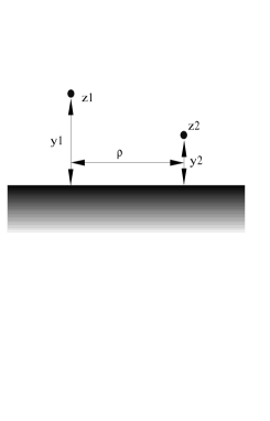
Figure 2: Parameters $y_{1}$, $y_{2}$ and $\rho$.

2.3 Classification of consistent boundary states

Physical systems described by CFT, such as the Ising model at criticality, usually have a finite number of conformally invariant, physically realisable boundary states corresponding to various boundary conditions. For example, in the Ising model there are three physical boundary states corresponding to all spins up, down, and free along the boundary. They are not only conformally invariant but satisfy some extra conditions. In this section we review Cardy’s classification of consistent boundary states[37], which uses the modular invariance of partition functions as the extra information. In the past several years the study of this method has been expanded enormously. Generalisations to various rational CFTs, including non-diagonal minimal theories[43, 44], superconformal models[45], coset models[46, 47], have been considered, and algebraic understanding of the method[48, 49, 50] has also been drastically improved. We shall not go into these recent developments but describe only the simplest diagonal case, following [37, 40].

The CFTs we analyse in this subsection are defined on an annulus. This geometry has a great advantage that the operators on the full plane (without boundary) may be employed without modification. This is due to the fact that in the radial quantisation, annulus arises as a portion of the full plane bounded by two concentric circles. One may use the conformal transformation $w=(T/\pi)\ln z$ and $\zeta=\exp(-2\pi iw/L)$ to map the boundary $z=\bar{z}$ of the half plane to the two circles bordering the annulus. This annulus may also be regarded as a cylinder with length $T$ and circumference $L$. On the $\zeta$-plane (annulus), the conformal invariance condition of the boundary (12) becomes

$$(L_{n}-\bar{L}_{-n})|B\rangle=0.$$ (21)

We shall call the boundary states $|B\rangle$ satisfying this condition as conformally invariant boundary states.

In ordinary rational conformal theories there is an important set of conformally invariant boundary states, called Ishibashi states. They are defined as

$$|j\rangle\!\rangle\equiv\sum_{M}|j;M\rangle\otimes U\overline{|j;M\rangle},$$ (22)

where $j$ is the label for representations, $M$ is the level in the conformal tower, and $U$ is an antiunitary operator which is the product of time reversal and complex conjugation. Ishibashi states are conformally invariant boundary states corresponding to conformal towers, and they form a basis spanning the space of boundary states. An important property of the Ishibashi states is that they diagonalise the closed string amplitudes and give characters for corresponding representations:

$$\langle\!\langle i|(q^{1/2})^{L_{0}+\bar{L}_{0}-c/12}|j\rangle\!\rangle=\delta_{ij}\chi_{i}(q).$$ (23)

These Ishibashi states are not normalisable, as the innerproducts between them (taking the limit $q\rightarrow 1$ in the expression above) are infinite.

The duality between open and closed string channels imposes a condition on the boundary states as follows (Fig.3). Suppose we have boundary conditions $\tilde{\alpha}$ and $\tilde{\beta}$ on the two ends of an open string. If these boundary conditions are physical, chiral representations labeled by $i$ appear in the bulk with non-negative integer multiplicities $n^{i}_{\tilde{\alpha}\tilde{\beta}}$. The partition function is then the sum of the chiral characters with the associated multiplicities,

$$Z_{\tilde{\alpha}\tilde{\beta}}(q)=\sum_{i}n^{i}_{\tilde{\alpha}\tilde{\beta}}\chi_{i}(q),$$ (24)

where $q=e^{-\pi L/T}$. This is the partition function in the open-string channel. In the closed-string channel, the partition function is nothing but the amplitude between two equal-time hypersurfaces,

$$Z_{\tilde{\alpha}\tilde{\beta}}=\langle\tilde{\alpha}|(\tilde{q}^{1/2})^{L_{0}+\bar{L}_{0}-c/12}|\tilde{\beta}\rangle,$$ (25)

where $\tilde{q}=e^{-4\pi T/L}$. Note that the Hamiltonian of our system is $2\pi(L_{0}+\bar{L}_{0}-c/12)/L$. The duality then demands

$$\sum_{i}n^{i}_{\tilde{\alpha}\tilde{\beta}}\chi_{i}(q)=\langle\tilde{\alpha}|(\tilde{q}^{1/2})^{L_{0}+\bar{L}_{0}-c/12}|\tilde{\beta}\rangle,$$ (26)

which is called Cardy’s consistency condition.

By solving this equation, one may find physical boundary conditions and express the associated consistent boundary states as particular linear combinations of the Ishibashi states[37]. Using the modular transformation of the characters $\chi_{i}(q)\rightarrow\chi_{i}(\tilde{q})=\sum_{j}S_{ij}\chi_{j}(q)$ under $\tau\rightarrow\tilde{\tau}=-1/\tau$, the left-hand side of (26) is written as

$$\sum_{i}n^{i}_{\tilde{\alpha}\tilde{\beta}}\chi_{i}(q)=\sum_{i,j}n^{i}_{\tilde{\alpha}\tilde{\beta}}S_{ij}\chi_{j}(\tilde{q}).$$ (27)

On the right-hand side, one may expand the boundary states with the Ishibashi states, as

$$\langle\tilde{\alpha}|(\tilde{q}^{1/2})^{L_{0}+\bar{L}_{0}-c/12}|\tilde{\beta}\rangle=\sum_{i,j}\langle\tilde{\alpha}|i\rangle\!\rangle\langle\!\langle i|(\tilde{q}^{1/2})^{L_{0}+\bar{L}_{0}-c/12}|j\rangle\!\rangle\langle\!\langle j|\tilde{\beta}\rangle=\sum_{j}\langle\tilde{\alpha}|j\rangle\!\rangle\langle\!\langle j|\tilde{\beta}\rangle\chi_{j}(\tilde{q}).$$ (28)

Equating the coefficients of the character functions on the both sides, we have

$$\sum_{i}S_{ij}n^{i}_{\tilde{\alpha}\tilde{\beta}}=\langle\tilde{\alpha}|j\rangle\!\rangle\langle\!\langle j|\tilde{\beta}\rangle.$$ (29)

Solutions to this equation are found by assuming the existence of a boundary state $|\tilde{0}\rangle$ satisfying $n^{i}_{\tilde{0}\tilde{\alpha}}=n^{i}_{\tilde{\alpha}\tilde{0}}=\delta^{i}_{\tilde{\alpha}}$ for any boundary condition $\tilde{\alpha}$. Letting $\tilde{\alpha}=\tilde{\beta}=\tilde{0}$ in (29), and using the positive-definiteness of $S_{0j}$ (which is always the case for unitary models) we have

$$|\tilde{0}\rangle=\sum_{j}\sqrt{S_{0j}}|j\rangle\!\rangle.$$ (30)

Next, putting $\tilde{\alpha}=\tilde{0}$ and $\tilde{\beta}\neq\tilde{0}$ in (29) and using the result above, we have

$$|\tilde{\alpha}\rangle=\sum_{j}\frac{S_{\alpha j}}{\sqrt{S_{0j}}}|j\rangle\!\rangle.$$ (31)

This result (31) includes the $\tilde{\alpha}=\tilde{0}$ case (30).

Let us see this result in the case of the critical Ising model. The operator contents $I=\phi_{1,1}=\phi_{2,3}$, $\sigma=\phi_{1,2}=\phi_{2,2}$, $\epsilon=\phi_{2,1}=\phi_{1,3}$ of the Kac formula are the identity, spin, and energy density operators, respectively. Substituting the modular S matrix for the Ising model characters (see App.B) we find consistent boundary states from (31) as

$$|\tilde{0}\rangle = |\tilde{I}\rangle=\frac{1}{\sqrt{2}}|I\rangle\!\rangle+\frac{1}{\sqrt{2}}|\epsilon\rangle\!\rangle+\frac{1}{\sqrt[4]{2}}|\sigma\rangle\!\rangle,$$ (34)

$$|\tilde{\epsilon}\rangle=\frac{1}{\sqrt{2}}|I\rangle\!\rangle+\frac{1}{\sqrt{2}}|\epsilon\rangle\!\rangle-\frac{1}{\sqrt[4]{2}}|\sigma\rangle\!\rangle,$$

$$|\tilde{\sigma}\rangle=|I\rangle\!\rangle-|\epsilon\rangle\!\rangle.$$

Since $|\tilde{I}\rangle$ and $|\tilde{\epsilon}\rangle$ differ only by the sign of $|\sigma\rangle\!\rangle$ associated with the spin operator, they are identified as the fixed boundary conditions ($|\uparrow\rangle$, $|\downarrow\rangle$). Which is up and which is down is purely a matter of choice. The remaining $|\tilde{\sigma}\rangle$ corresponds to the free boundary condition $|F\rangle$.

(a) Open string channel            (b) Closed string channel

Figure 3: The open-string channel (a) and the closed-string channel (b) are related by the duality exchanging the directions of time and space. The equivalence of the partition functions calculated in each channel leads to the constraints (26) on the boundary states.

2.4 Verlinde formula

One of the most remarkable properties of genus one conformal field theories is that fusion rules can be determined by the modular transformations of the operator contents. This is highly non-trivial since fusion is a local property of operators whereas modular transformations are obviously global. The relation between fusion and modular transformations is summarised in the form of the celebrated Verlinde formula [38]:

$$N_{ij}{}^{k}=\sum_{m}\frac{S_{im}S_{jm}\bar{S}_{mk}}{S_{0m}},$$ (35)

where $N_{ij}{}^{k}$ is the fusion matrix in $\phi_{i}\times\phi_{j}=\sum_{k}N_{ij}{}^{k}\phi_{k}$ and $S_{ij}$ is the modular S matrix $\chi_{i}(-1/\tau)=\sum_{j}S_{ij}\chi_{j}(\tau)$. The index $0$ stands for the vacuum representation. The proof of this equation is due to the underlying quantum group structure applied to genus one manifold[51, 52]. See also [53] for a more recent review. Using $SS^{\dagger}=1$, the above relation may be written in the form

$$\sum_{k}N_{ij}{}^{k}S_{km}=\frac{S_{im}}{S_{0m}}S_{jm},$$ (36)

meaning that the fusion matrix is diagonalised by the modular S matrix.

In boundary theory, substituting (31) into the duality relation (29) we have

$$\sum_{i}S_{ij}n^{i}_{\tilde{\alpha}\tilde{\beta}}=S_{\alpha j}S_{\beta j}/S_{0j}.$$ (37)

Comparing this with (36), it is concluded that[37]

$$N_{ij}{}^{k}=n^{k}_{ij},$$ (38)

that is, the multiplicity of the representations appearing in the bulk is identical to the fusion coefficient for the operators associated to the boundary states.

2.5 Boundary operators and critical percolation

The mirroring method reviewed in Sec.2.2 naturally introduces another important object in boundary CFT, called a boundary operator[39], which is defined through the OPE of two bulk operators, one on the upper and the other on the lower half plane,

$$\phi_{i}(z)\phi_{j}(z^{*})\sim\sum_{k}(z-z^{*})^{(h_{k}-h_{i}-h_{j})}N_{ij}{}^{k}\phi_{B,k}(x),$$ (39)

where $x=(z+z^{*})/2$. The $\phi_{B,k}(x)$ are the boundary operators which reside on the boundary. Such a boundary operator may change the boundary condition when inserted. The operator changing the boundary state from $\tilde{\alpha}$ to $\tilde{\beta}$ is denoted as $\phi_{(\tilde{\alpha}\tilde{\beta})}$.

The critical bond percolation problem in statistical physics is an example which is solved using boundary operators. Since this is often discussed in the context of logarithmic CFTs, we shall review it here briefly[17, 40, 54].

The problem we want to solve is defined as follows. We consider a lattice of horizontal length $a\ell$, vertical length $b\ell$ and spacing $\ell$, and set electrodes on the left and right sides of the lattice. We start placing conducting needles randomly on the grid, and observe if electric current can run between the two electrodes (horizontal percolation). Obviously, when we put no needle on the lattice there is no way the current can run through, and when all the grids are filled with conducting needles the percolation has readily been achieved. Thus there must be some occupation probability $p$ between $0$ and $1$ which is barely sufficient to achieve the percolation. We may take the thermodynamic limit of this system (letting $\ell\rightarrow 0$ and $a\ell$, $b\ell$ fixed). Then there is a critical occupation probability $p_{c}$ such that the horizontal percolation probability $\pi_{h}$ is one for $p>p_{c}$ and $\pi_{h}=0$ for $p<p_{c}$. The system at $p=p_{c}$ is called the critical bond percolation. At $p=p_{c}$, $\pi_{h}$ still depends on the aspect ratio $r=a/b$. Our problem is to find $\pi_{h}$ as a function of $r$.

This percolation problem is translated into $Q\rightarrow 1$ limit of the Q-state Potts model in two dimension[55, 56]. The interaction energy of the Q-state Potts model is $J\sum_{\langle ij\rangle}\delta_{\sigma_{i}\sigma_{j}}$, where the sum is over nearest-neighbours and the indices $i$ and $j$ take one of the Q states. The partition function of the Q-state Potts model is then

$$Z=\sum_{\mbox{\scriptsize config}}\prod_{\langle ij\rangle}\exp\left\{-\beta J\delta_{\sigma_{i}\sigma_{j}}\right\}.$$ (40)

Defining $1/(1-p)=e^{-\beta J}$, one may rewrite this partition function as

$$Z=\sum_{\mbox{\scriptsize activation}}p^{B}(1-p)^{b-B}Q^{N_{c}},$$ (41)

where $b$ is the number of bonds, $B$ is the number of activated bonds (needles), and $N_{c}$ is the number of disjoint clusters. The Q-state Potts model has been mapped into a system with active bonds of Q possible colours (probability $=p$) and inert bonds (probability$=1-p$). It is now obvious that the critical percolation is realised by taking $Q\rightarrow 1$ limit of this system.

The relation between the Q-state Potts models and the ${\cal M}(m+1,m)$ unitary minimal series ($m=3$ is the Ising model) is well established for $Q=2,3,4$. The correspondence is given by $Q=4\cos^{2}(\pi/(m+1))$ for these models. Extrapolating this formula for arbitrary value of $m$, the bond percolation problem then correspond to the minimal model of ${\cal M}(3,2)$, whose central charge is $c=0$. Using this correspondence, the percolation problem is described in a boundary CFT language as follows. Let us consider a rectangle with a pair of opposing sides having free boundary condition $\tilde{f}$ (Fig.4). The remaining two sides have fixed boundary conditions $\tilde{\alpha}$ and $\tilde{\beta}$, with fixed ‘colours’ out of the Q possible colours of the activated bonds. Such a configuration is realised by inserting four boundary (changing) operators at the four corners of the rectangle. The boundary operator $\phi_{(\tilde{\alpha}\tilde{f})}$, which changes a fixed boundary condition to the free boundary condition, is identified as $\phi_{2,1}$ by analogy with the Q-state Potts models of $Q=2,3,4$.

Figure 4: Horizontal bond percolation is modelled by a rectangle with the free boundary condition on the top and bottom sides, and fixed boundary conditions on the left and right sides.

The crossing probability $\pi_{h}$ is obtained by calculating the partition functions for the configurations

$$\left(\begin{picture}(30.0,15.0)\put(5.0,-7.0){\line(0,1){15.0}} \put(25.0,-7.0){\line(0,1){15.0}} \put(5.0,3.0){\line(1,0){5.0}} \put(10.0,3.0){\line(0,-1){5.0}} \put(10.0,-2.0){\line(1,0){5.0}} \put(15.0,-2.0){\line(0,-1){5.0}} \put(15.0,-7.0){\line(1,0){5.0}} \put(20.0,-7.0){\line(0,1){5.0}} \put(20.0,-2.0){\line(1,0){5.0}} \put(2.0,0.5){$\tilde{\alpha}$} \put(26.0,0.5){$\tilde{\alpha}$} \put(15.0,-1.0){$\tilde{\alpha}$} \end{picture}\right)+\left(\begin{picture}(30.0,15.0)\put(5.0,-7.0){\line(0,1){15.0}} \put(25.0,-7.0){\line(0,1){15.0}} \put(5.0,3.0){\line(1,0){5.0}} \put(10.0,3.0){\line(0,-1){5.0}} \put(10.0,-2.0){\line(1,0){5.0}} \put(15.0,-2.0){\line(0,-1){5.0}} \put(15.0,-7.0){\line(1,0){5.0}} \put(15.0,3.0){\line(1,0){5.0}} \put(20.0,-2.0){\line(0,1){5.0}} \put(20.0,-2.0){\line(1,0){5.0}} \put(2.0,0.5){$\tilde{\alpha}$} \put(26.0,0.5){$\tilde{\alpha}$} \put(11.0,-6.0){$\tilde{\alpha}$} \put(16.0,4.0){$\tilde{\alpha}$} \end{picture}\right)-\left(\begin{picture}(30.0,15.0)\put(5.0,-7.0){\line(0,1){15.0}} \put(25.0,-7.0){\line(0,1){15.0}} \put(5.0,3.0){\line(1,0){5.0}} \put(10.0,3.0){\line(0,-1){5.0}} \put(10.0,-2.0){\line(1,0){5.0}} \put(15.0,-2.0){\line(0,-1){5.0}} \put(15.0,-7.0){\line(1,0){5.0}} \put(15.0,3.0){\line(1,0){5.0}} \put(20.0,-2.0){\line(0,1){5.0}} \put(20.0,-2.0){\line(1,0){5.0}} \put(2.0,0.5){$\tilde{\alpha}$} \put(26.0,0.5){$\tilde{\beta}$} \put(11.0,-6.0){$\tilde{\alpha}$} \put(16.0,4.0){$\tilde{\beta}$} \end{picture}\right)$$ (42)

and taking the limit $Q\rightarrow 1$ (that is, $\tilde{\alpha}=\tilde{\beta}$) afterwards. Note that in this limit the last two terms cancel and only the first one (realising the percolation) remains. If we write the partition function for the configurations with the boundary condition $\tilde{\alpha}$ on the left and $\tilde{\beta}$ on the right as $Z_{\tilde{\alpha}\tilde{\beta}}$, the crossing probability is given by

$$\pi_{h}=\lim_{Q\rightarrow 1}(Z_{\tilde{\alpha}\tilde{\alpha}}-Z_{\tilde{\alpha}\tilde{\beta}}),$$ (43)

since the first two terms of the graphical representation (42) are $Z_{\tilde{\alpha}\tilde{\alpha}}$ and the last one is $Z_{\tilde{\alpha}\tilde{\beta}}$. These partition functions for particular boundary conditions are given by the four-point functions of the boundary operators. Then up to a multiplicative constant we have

$$\pi_{h} \sim \langle\phi_{(\tilde{f}\tilde{\alpha})}(x_{1})\phi_{(\tilde{\alpha}\tilde{f})}(x_{2})\phi_{(\tilde{f}\tilde{\beta})}(x_{3})\phi_{(\tilde{\beta}\tilde{f})}(x_{4})\rangle_{Q=1}$$ (44)

$$= \langle\phi_{12}(x_{1})\phi_{12}(x_{2})\phi_{12}(x_{3})\phi_{12}(x_{4})\rangle_{Q=1}.$$

The four-point function $\langle\phi_{12}(x_{1})\phi_{12}(x_{2})\phi_{12}(x_{3})\phi_{12}(x_{4})\rangle$ is found by solving a second order ordinary differential equation. Introducing the cross ratio $\eta=[(z_{4}-z_{3})(z_{2}-z_{1})]/[(z_{3}-z_{1})(z_{4}-z_{2})]$, where $z_{i}$ are the coordinates after the Schwartz-Christoffel transformation $x_{i}\rightarrow z_{i}$ mapping the interior of the rectangle to the upper half plane, the differential equation for $\pi_{h}(\eta)=g(\eta)$ is

$$\eta(1-\eta)\frac{d^{2}g(\eta)}{d\eta^{2}}+\frac{2(1-2\eta)}{3}\frac{dg(\eta)}{d\eta}=0.$$ (45)

This differential equation has two independent solutions. One of them is $g(\eta)=const$. The other is

$$g(\eta)=\eta^{1/3}F(\frac{1}{3},\frac{2}{3},\frac{4}{3};\eta).$$ (46)

The crossing probability $\pi_{h}$ is a linear combination of the two solutions. The coefficients are determined by demanding $\pi_{h}\rightarrow 1$ when the rectangle is infinitely narrow and $\pi_{h}\rightarrow 0$ when it is infinitely wide. The solution is then

$$\pi_{h}(\eta)=\frac{3\Gamma(2/3)}{\Gamma(1/3)^{2}}\eta^{1/3}F(\frac{1}{3},\frac{2}{3},\frac{4}{3};\eta).$$ (47)

This analytic result is compared with numerical calculations and exhibits excellent agreement[17, 57, 58]. Although the extrapolation of the $Q\neq 1$ results to $Q\rightarrow 1$ may seem somewhat speculative, this agreement justifies the method of the analysis as well as the underlying concepts such as conformal invariance and boundary operators.

Finally we emphasise that this CFT at $c=0$ is not the minimal model of ${\cal M}(3,2)$, which consists only of the identity operator. Recall that the differential equation (45) has two independent solutions, one corresponds to the conformal block $\phi_{1,1}$ and the other to $\phi_{1,3}$. Obviously, the former solution is the constant and the latter is (46). If we were dealing with ${\cal M}(3,2)$ minimal model, the solution (46) should have been discarded since it is associated to the operator outside the Kac table. Hence the percolation problem must be considered in the framework of a CFT with extended conformal grid, possibly to ${\cal M}(9,6)$[32, 54]. From this example we may expect the existence of bona-fide CFTs which are not minimal models but something that should be called ‘next-to-minimal’ models, which may well include logarithmic operators[59]. The existence of such statistical models is one of the biggest reasons for studying logarithmic CFTs with boundary.

3 Logarithmic CFT with boundary

In this section we discuss logarithmic conformal field theories with boundary. Probably the biggest motivation for the study of such theories is the existence of a number of statistical systems which are conjectured to be modelled by logarithmic CFTs, where the finite size effect may not be negligible if the system has a boundary. There are also examples in which boundary operators play an essential role, as is mentioned at the end of the last section. As logarithmic CFTs are in general non unitary, being far from boundary does not guarantee the irrelevance of the boundary effect. Once we have a boundary, its effect may change the system globally. Therefore the study of boundary effect seems to be extremely important for a proper CFT description of non-unitary systems. Also, in string theory context, there are several examples such as D-brane recoil[29, 30] and dimensional reduction[60], where logarithmic operators are claimed to play important roles. These are less established theories than the statistical model examples, and certainly more investigation is required. If they turn out to be correct descriptions, the boundary theory of such systems will be important since open strings and branes necessarily involve world sheet boundaries.

When we try to apply standard techniques of boundary CFT to logarithmic cases, several unusual features arise. In the following we shall see such results for the $c=-2$ logarithmic CFT. In the next subsection we calculate correlation functions in the presence of boundary and argue that logarithmic behaviour is unavoidable either near or away from the boundary[34]. In Subsec.3.2 we review free-field representation of the $c=-2$ model, following [7, 61, 62]. Even on genus one manifold without boundary, the logarithmic CFT at $c=-2$ is somewhat pathological, in that the fusion matrix is not diagonalisable and thus the Verlinde formula fails. We shall review this in Sec. 3.3. As Cardy’s method depends largely on the modular properties of CFT, the classification of boundary states in logarithmic CFT does not go straightforwardly. However, we can still find ‘good’ boundary states with consistent modular properties, as is discussed in Sec. 3.4.

3.1 Boundary correlation functions in LCFT

The CFT at $c=c_{2,1}=-2$ is one of the logarithmic CFTs that have been studied most intensively and are so far best understood. This was used by Gurarie[5] to discuss the importance of logarithmic operators, and it is also claimed that certain universality classes of two-dimensional statistical models (such as critical polymers in the dense phase[3]) are described by this theory. Let us start by discussing operator contents of this theory, assuming that they are given by extending the Virasoro minimal models. Of course the Kac determinant must be reconsidered to get a proper formula consistent with the non-trivial Jordan cell[32, 63]. However we shall adopt the original formula here, as it still contains some truth at least for the pre-logarithmic part.

Usually the operator content of the ${\cal M}(p,p^{\prime})$ minimal model (we assume $p>p^{\prime}$) is restricted to $\phi_{r,s}$ such that $0<r<p^{\prime}$, $0<s<p$ (and also $pr>p^{\prime}s$ to avoid the double counting of identical operators). Since the Kac table for $(p,p^{\prime})=(2,1)$ is empty, the border of the grid must be extended in order to have a non-trivial theory. Note that the Kac formula of conformal dimension $h_{r,s}$ for ${\cal M}(p,p^{\prime})$ minimal model,

$$h_{r,s}=\frac{(pr-p^{\prime}s)^{2}-(p-p^{\prime})^{2}}{4pp^{\prime}},$$ (48)

is invariant for the “rescaling” $p\rightarrow lp$ and $p^{\prime}\rightarrow lp^{\prime}$ for some natural number $l$. The table of conformal dimensions for the extended ${\cal M}(2,1)$ minimal model is

	$s$
$r$	$1$	$2$	$3$	$4$	$5$	$6$	$7$	$8$	$9$	$10$	$11$	$12$
$1$	$0$	$-1/8$	$0$	$3/8$	$1$	$15/8$	$3$	$35/8$	$6$	$63/8$	$10$	$\cdots$
$2$	$1$	$3/8$	$0$	$-1/8$	$0$	$3/8$	$1$	$15/8$	$3$	$35/8$	$6$
$3$	$3$	$15/8$	$1$	$3/8$	$0$	$-1/8$	$0$	$3/8$	$1$	$15/8$	$3$
$4$	$6$	$35/8$	$3$	$15/8$	$1$	$3/8$	$0$	$-1/8$	$0$	$3/8$	$1$
$5$	$10$	$63/8$	$6$	$35/8$	$3$	$15/8$	$1$	$3/8$	$0$	$-1/8$	$0$
$6$	$\cdots$											$\cdots$

We shall restrict the contents to $0<r<3$, $0<s<6$, that is, we consider the ‘next-to-minimal’ model ${\cal M}(6,3)$. It has been shown by a free-field representation that these operators indeed close under the fusion rule.

The operators $\phi_{1,1}$, $\phi_{1,3}$, and $\phi_{1,5}$ belong to a degenerate ‘logarithmic’ block and are expected to be governed by unusual Ward identities[63]. However, $\mu=\phi_{1,2}$ and $\nu=\phi_{1,4}$ are normal (pre-logarithmic) operators and therefore satisfy ordinary conformal Ward identities. This enables us to calculate boundary $n$-point functions involving $\mu$ and $\nu$[34, 64], using the mirroring method described in Subsec.2.2. Let us see this in a simple example, boundary $2$-point function of the spin $-1/8$ operators $\langle\mu\mu\rangle_{B}$[34]. As the boundary $n$-point functions are equivalent to chiral $2n$-point functions, in our case we have

$$\langle\mu(z_{1},\bar{z}_{1})\mu(z_{2},\bar{z}_{2})\rangle_{B}=\langle\mu(z_{1})\mu(z_{2})\mu(z_{1}^{*})\mu(z_{2}^{*})\rangle_{chiral}.$$ (49)

Since $\mu=\phi_{1,2}$, this chiral $4$-point function satisfies a second order differential equation, which reduces to a hypergeometric differential equation after Möbius transformations. The solution is easily found as

$$\langle\mu(z_{1},\bar{z}_{1})\mu(z_{2},\bar{z}_{2})\rangle_{B}$$

$$=|z_{1}-z_{2}^{*}|^{1/2}z^{1/4}(1-z)^{1/4}\left\{AF(\frac{1}{2},\frac{1}{2},1;z)+BF(\frac{1}{2},\frac{1}{2},1;1-z)\right\},$$ (50)

where $z$ is the cross ratio,

$$z=\frac{(z_{1}-z_{2})(z_{1}^{*}-z_{2}^{*})}{(z_{1}-z_{2}^{*})(z_{1}^{*}-z_{2})}=\frac{|z_{1}-z_{2}|^{2}}{|z_{1}-z_{2}^{*}|^{2}},$$ (51)

and $A$ and $B$ are constants to be determined by boundary conditions. Note that this is a single-valued function since $z$ is always real and $0<z<1$. The function $F(1/2,1/2,1;z)$ is a hypergeometric function of Gaussian type and reduces to the complete elliptic integral

$$\frac{\pi}{2}F(\frac{1}{2},\frac{1}{2},1;k^{2})=K(k)=\int_{0}^{\pi/2}\frac{d\theta}{\sqrt{1-k^{2}\sin^{2}\theta}}.$$ (52)

If the points $z_{1}$ and $z_{2}$ are away from the boundary but the separation is kept fixed, we have $z\rightarrow 0$ and then

$$\langle\mu(z_{1},\bar{z}_{1})\mu(z_{2},\bar{z}_{2})\rangle_{B}\rightarrow A|z_{1}-z_{2}|^{1/2}+2B|z_{1}-z_{2}|^{1/2}\ln|z_{1}-z_{2}|.$$ (53)

The first term is the same as the bulk $2$-point function. Hence, we may let $B=0$ if we want to recover the bulk result by letting $z_{1}$ and $z_{2}$ away from the boundary. However, there is no physical motivation to do so because our theory is not unitary and the $2$-point function grows with the separation. That is, being away from the boundary does not guarantee the negligibility of the boundary effect.

If the two operators are close to the boundary, we have $z\rightarrow 1$ and then $F(\frac{1}{2},\frac{1}{2},1;1-z)\rightarrow 1$. The correlation function is dominated by the first term,

$$\langle\mu(z_{1},\bar{z}_{1})\mu(z_{2},\bar{z}_{2})\rangle_{B}\sim 2A|z_{1}-z_{1}^{*}|^{1/2}\ln\frac{|z_{1}-z_{1}^{*}|}{|z_{1}-z_{2}|},$$ (54)

displaying a logarithmic behaviour. We conclude that the $2$-point function of pre-logarithmic operators exhibit logarithmic divergence either away from or close to the boundary.

3.2 Triplet $c=-2$ model in free-field representation

Extension of the Kac table discussed in the previous subsection allows us to use differential equations for correlation functions and in some situations (when the correlators involve non-logarithmic operators) we can find explicit form of correlation functions with or without boundary. Such a method is quite powerful and is apparently a correct approach at least for some cases. For example, in the percolation problem reviewed in Subsec.1.5, we have used a solution of a differential equation associated to an operator outside the Kac table, and the result is supported by a remarkable agreement with numerical calculations.

However, it is desirable to start a theory from a more solid ground, as we do not know to what extent the results of the unitary minimal models may be generalised to logarithmic cases without modification. In $c=-2$ logarithmic CFT, a construction based on a free-field representation does exist, and the so-called triplet model has been shown to be realised by symplectic fermions. In this subsection we review the free-field representation of this model following [61, 62] and collect basic results needed for following discussions. For more complete descriptions readers are referred to the original papers[61, 62]. See also [6, 7, 65] and the lecture note by Gaberdiel[33].

Symplectic fermions have the same central charge $c=-2$ as the simple ghost system whose action is

$$S=\frac{1}{\pi}\int d^{2}z(\eta\bar{\partial}\xi+\bar{\eta}\partial\bar{\xi}),$$ (55)

where $\eta$ and $\xi$ are fermionic ghosts with conformal dimensions $h_{\eta}=1$ and $h_{\xi}=0$. The operator products are

$$\eta(z)\xi(w)\sim\xi(z)\eta(w)\sim 1/(z-w),$$ (56)

reflecting the Grassmannian nature of the operators. Symplectic fermions are introduced as operators of conformal dimensions $h_{\chi^{\pm}}=1$, defined as

$$\chi^{+}\equiv\eta,\;\;\chi^{-}\equiv\partial\xi.$$ (57)

The mode expansions,

$$\chi^{\pm}(z)=\sum_{k\in Z}\chi^{\pm}_{k}z^{-k-1},$$ (58)

define the mode operators $\chi^{\pm}_{k}$ with anti-commutation relations,

$$\{\chi^{\alpha}_{m},\chi^{\beta}_{n}\}=md^{\alpha\beta}\delta_{m+n},$$ (59)

where $d^{\alpha\beta}$ is antisymmetric and $d^{\pm\mp}=\pm 1$. These symplectic fermions differ from the $\eta$-$\xi$ simple ghost system by the zero-mode of $\xi$. The absence of $\xi_{0}$ enhances the symmetry and realises the triplet model at $c=-2$.

Orbifold structure is endowed by considering twisted sectors as well as the untwisted sector[3, 61, 62]. The twisted sectors are built on the vacuum by operating with a twisting field $\sigma_{k/N}$, and the resulting theory becomes $Z_{N}$ invariant. It is argued that the $Z_{N}$ orbifold model constructed like this has a W-algebra of type ${\cal W}(2,3,N(N+1)/2,N(N+1)/2)$[65]. In the case of $N=2$ the model possesses ${\cal W}(2,3,3,3)$ symmetry which is generated by the stress tensor

$$T(z)=:\chi^{-}(z)\chi^{+}(z):+\lambda(\lambda-1)/2z^{2},$$ (60)

where $\lambda=0$ for the untwisted and $\lambda=1/2$ for the twisted sector, and a triplet of W-fields with conformal dimension 3,

$$W^{0}=-\frac{1}{2}(:\partial\chi^{+}(z)\chi^{-}(z):+:\partial\chi^{-}(z)\chi^{+}(z):),$$

$$W^{\pm}=:\partial\chi^{\pm}(z)\chi^{\pm}(z):.$$ (61)

Virasoro operators and $W$-mode operators are found from these as

$$L_{n}=\frac{1}{2}d_{\alpha\beta}\sum_{m\in Z+\lambda}:\chi^{\alpha}_{m}\chi^{\beta}_{n-m}:+\frac{\lambda(\lambda-1)}{2}\delta_{n0},$$ (62)

and

$$W^{0}_{n} = -\frac{1}{2}\sum_{j\in Z+\lambda}j\left\{:\chi^{+}_{n-j}\chi^{-}_{j}:+:\chi^{-}_{n-j}\chi^{+}_{j}:\right\},$$

$$W^{\pm}_{n} = \sum_{j\in Z+\lambda}j\chi^{\pm}_{n-j}\chi^{\pm}_{j}.$$ (63)

In the following we only consider the $N=2$ case which is called the triplet model for an obvious reason.

The representations with conformal weights $-1/8$, $0$, $3/8$ and $1$ expected from the Kac table at $c_{2,1}=-2$ are associated to the Fock space representations of the symplectic fermions as follows[7, 33, 62]. The ground state of the twisted sector which is obtained by operating with $\sigma_{1/2}$ on the vacuum is denoted by $\mu$. This $\mu$ has conformal weight $-1/8$, and then the singlet representation ${\cal V}_{-1/8}$ is defined as states built on $\mu$. The doublet of the states $\nu^{\pm}\equiv\chi^{\pm}_{-1/2}\mu$ has conformal dimension $3/8$ and this is the highest-weight states of the doublet representation ${\cal V}_{3/8}$. Since ${\cal V}_{3/8}$ corresponds to $\phi_{1,4}$ or $\phi_{2,2}$ in the Kac table, the correlation functions involving ${\cal V}_{3/8}$ satisfy fourth order differential equations, whose solutions represent two conformal blocks for $\nu^{+}$ and $\nu^{-}$ each. The representations belonging to the untwisted sector are more complicated. Let $\omega$ be a state annihilated by operations with $\chi^{\pm}_{n>0}$. Then there are four ground states, $\omega$, $\theta^{\pm}=-\chi^{\pm}_{0}\omega$, and $\Omega=\chi^{-}_{0}\chi^{+}_{0}\omega=L_{0}\omega$. As $\Omega$ is annihilated by further operations with zero modes, it is identified as the Möbius invariant vacuum. The irreducible vacuum representation ${\cal V}_{0}$ is built on the ground state $\Omega$. Similarly, the irreducible doublet representation ${\cal V}_{1}$ at $h=1$ is built on the doublet $\psi^{\pm}=\chi^{\pm}_{-1}\Omega$.

These four representations ${\cal V}_{-1/8}$, ${\cal V}_{3/8}$, ${\cal V}_{0}$ and ${\cal V}_{1}$ do not close under the fusion and thus extra representations are needed. The ‘reducible but indecomposable’ representation ${\cal R}_{0}$ is obtained by extending the vacuum ${\cal V}_{0}$ to include $\omega$, $L_{-1}\omega$ and $W^{a}_{-1}\omega$ as well as $\Omega$. The two bosonic ground states $\Omega$ and $\omega$ span a two-dimensional Jordan cell on the action of $L_{0}$, forming a ‘logarithmic pair.’ The representation ${\cal R}_{1}$ is obtained likewise, by extending ${\cal V}_{1}$ to include $\phi^{\pm}=\chi^{\pm}_{-1}\omega$ and $\xi^{\pm}=-L_{1}\phi^{\pm}$ in addition to $\psi^{\pm}=\chi^{\pm}_{-1}\Omega$. The doublet states $\psi^{\pm}$ and $\phi^{\pm}$ form a logarithmic pair at $h=1$. The four representations ${\cal V}_{-1/8}$, ${\cal V}_{3/8}$, ${\cal R}_{0}$ and ${\cal R}_{1}$ close under the fusion.

The representations in the triplet model are summarised as follows:

Twisted sector

$$\begin{array}[]{ccc}\mu&\rightarrow&{\cal V}_{-1/8}\\ \nu^{\pm}\equiv\chi^{\pm}_{-1/2}\mu&\rightarrow&{\cal V}_{3/8}\end{array}$$

Untwisted sector

$$\begin{array}[]{ccc}\Omega&\rightarrow&{\cal V}_{0}\\ \psi^{\pm}\equiv\chi^{\pm}_{-1}\Omega&\rightarrow&{\cal V}_{1}\end{array}$$

$$\begin{array}[]{ccc}\omega,\;\;\Omega,\;\;L_{-1}\omega,\;\;W^{a}_{-1}\omega&\rightarrow&{\cal R}_{0}\\ \phi^{\pm}\equiv\chi^{\pm}_{-1}\omega,\;\;\psi^{\pm},\;\;\xi^{\pm}\equiv-L_{1}\phi^{\pm}&\rightarrow&{\cal R}_{1}\end{array}$$

3.3 Fusion rules and modular invariants

The fusion rules of the $c=-2$ triplet model are calculated both in the algebraic method[6, 33] and the free-field method[62] to be

$$\begin{array}[]{lll}{\cal R}_{i}\times{\cal R}_{j}&=2{\cal R}_{0}+2{\cal R}_{1}&i,j=0,1,\\ {\cal R}_{i}\times{\cal V}_{j}&={\cal R}_{0}&(i,j)=(0,0),(1,1),\\ &={\cal R}_{1}&(i,j)=(0,1),(1,0),\\ &=2{\cal V}_{-1/8}+2{\cal V}_{3/8}&i=0,1;j=-\frac{1}{8},\frac{3}{8},\\ {\cal V}_{i}\times{\cal V}_{j}&={\cal V}_{0}&(i,j)=(0,0),(1,1),\\ &={\cal V}_{1}&(i,j)=(0,1),(1,0),\\ &={\cal V}_{-1/8}&(i,j)=(0,-\frac{1}{8}),(1,\frac{3}{8}),\\ &={\cal V}_{3/8}&(i,j)=(1,-\frac{1}{8}),(0,\frac{3}{8}),\\ &={\cal R}_{0}&(i,j)=(-\frac{1}{8},-\frac{1}{8}),(\frac{3}{8},\frac{3}{8}),\\ &={\cal R}_{1}&(i,j)=(-\frac{1}{8},\frac{3}{8}),(\frac{3}{8},-\frac{1}{8}).\end{array}$$ (64)

Since the four representations ${\cal R}_{0}$, ${\cal R}_{1}$, ${\cal V}_{-1/8}$ and ${\cal V}_{3/8}$ close under this fusion rule, the triplet model can be regarded as a rational conformal field theory, with a weakened definition of rationality[6].

What is unusual about this fusion rule is that it is not diagonalisable. This is in a sharp contrast with ordinary rational theories, where fusion matrices are always diagonalised with modular S matrices through the Verlinde formula. As is expected from the failure of the Verlinde formula, the characters of the triplet model are quite unusual as well. They are calculated in [6, 62, 66, 67] as

$$\chi_{{\cal V}_{0}}(\tau)=\frac{\Theta_{1,2}(\tau)}{2\eta(\tau)}+\frac{1}{2}\eta(\tau)^{2},$$

$$\chi_{{\cal V}_{1}}(\tau)=\frac{\Theta_{1,2}(\tau)}{2\eta(\tau)}-\frac{1}{2}\eta(\tau)^{2},$$

$$\chi_{{\cal V}_{-1/8}}(\tau)=\frac{\Theta_{0,2}(\tau)}{\eta(\tau)},$$

$$\chi_{{\cal V}_{3/8}}(\tau)=\frac{\Theta_{2,2}(\tau)}{\eta(\tau)},$$

$$\chi_{{\cal R}_{0}}(\tau)=\chi_{{\cal R}_{1}}(\tau)=\frac{2\Theta_{1,2}(\tau)}{\eta(\tau)},$$ (65)

where $\Theta_{k,l}(\tau)$ and $\eta(\tau)$ are Jacobi theta functions and Dedekind eta function, respectively (see App.B for definitions). Note that these character functions are not independent, $\chi_{{\cal R}_{0}}=\chi_{{\cal R}_{1}}=2\chi_{{\cal V}_{0}}+2\chi_{{\cal V}_{1}}$. The mutual dependence of the character functions is reminiscent of the minimal Virasoro theories with extra symmetry (such as the three-state Potts model). What is more pathological is the modular transformation property of these characters. Since $\eta(\tau)^{2}\rightarrow\eta(\tilde{\tau})^{2}=-i\tau\eta(\tau)^{2}$ as $\tau\rightarrow\tilde{\tau}=-1/\tau$, the character functions do not transform each other linearly under the modular transformation.

Nevertheless, we may construct a modular-invariant partition function from these character functions[7, 33]. Indeed,

$$Z(\tau,\bar{\tau}) = \chi_{{\cal V}_{-1/8}}\bar{\chi}_{{\cal V}_{-1/8}}+\chi_{{\cal V}_{3/8}}\bar{\chi}_{{\cal V}_{3/8}}+2\chi_{{\cal V}_{0}}\bar{\chi}_{{\cal V}_{0}}+2\chi_{{\cal V}_{0}}\bar{\chi}_{{\cal V}_{1}}+2\chi_{{\cal V}_{1}}\bar{\chi}_{{\cal V}_{0}}+2\chi_{{\cal V}_{1}}\bar{\chi}_{{\cal V}_{1}}$$ (66)

$$= \frac{1}{|\eta(\tau)|^{2}}\sum_{k=0}^{3}|\Theta_{k,2}(\tau)|^{2},$$

is easily verified to be invariant under both $\tau\rightarrow-1/\tau$ and $\tau\rightarrow\tau+1$.

3.4 Boundary states at $c=-2$

As the Verlinde formula fails for the $c=-2$ triplet model, we can expect a difficulty applying the method illustrated in Sec.2.3 to this model. Indeed, when we try to find consistent boundary states as linear combinations of Ishibashi states, we immediately come across ambiguity due to the degeneracy of characters[34, 68]. On the other hand, since $c=-2$ theory is expected to model statistical systems such as polymers, it is not conceivable that this theory has no consistent boundary states. In this subsection we see that such boundary states with consistent modular properties can be found if we use the symplectic fermion representation of the triplet model[35].

Our starting point is to notice that the right hand side of the duality condition,

$$\sum_{i}n^{i}_{\tilde{\alpha}\tilde{\beta}}\chi_{i}(q)=\langle\tilde{\alpha}|(\tilde{q}^{1/2})^{L_{0}+\bar{L}_{0}-c/12}|\tilde{\beta}\rangle,$$ (67)

may be expanded with any basis of boundary states, not necessarily Ishibashi states. Since Ishibashi states rely on well-defined conformal towers, we want to express consistent boundary states in terms of a more ‘sound’ basis. As the boundary must be diffeomorphism invariant, the basis boundary states must satisfy

$$\left(L_{m}-\bar{L}_{-m}\right)|B\rangle=0.$$ (68)

In string theory, solutions to this condition are well known for boson, fermion and ghost fields, and are found in the form of coherent states. Let us find such coherent states for the symplectic fermions, following the similar procedure for Majorana fermions[69]. We shall demand vanishing of the boundary term in the action (55). In terms of the mode operators of symplectic fermions, this leads to the conditions on the boundary states,

$$\left(\chi^{\pm}_{m}-e^{\pm i\phi}\bar{\chi}^{\pm}_{-m}\right)|B\rangle=0,$$ (69)

$$\langle B|\left(\chi^{\pm}_{m}-e^{\pm i\phi}\bar{\chi}^{\pm}_{-m}\right)=0,$$ (70)

where $\phi$ is a phase factor reflecting the $U(1)$ symmetry of the system. The states satisfying this condition are easily found to be

$$|B_{0\phi}\rangle = \exp\left(\sum_{k>0}\frac{e^{i\phi}}{k}\chi^{-}_{-k}\bar{\chi}^{+}_{-k}+\frac{e^{-i\phi}}{k}\bar{\chi}^{-}_{-k}\chi^{+}_{-k}\right)|0_{\phi}\rangle,$$ (71)

$$\langle B_{0\phi}| = \langle 0_{\phi}|\exp\left(\sum_{k>0}\frac{e^{i\phi}}{k}\chi^{-}_{k}\bar{\chi}^{+}_{k}+\frac{e^{-i\phi}}{k}\bar{\chi}^{-}_{k}\chi^{+}_{k}\right),$$ (72)

where the vacua satisfy

$$\left(\chi^{\pm}_{0}-e^{\pm i\phi}\bar{\chi}^{\pm}_{0}\right)|0_{\phi}\rangle=0,$$

$$\langle 0_{\phi}|\left(\chi^{\pm}_{0}-e^{\pm i\phi}\bar{\chi}^{\pm}_{0}\right)=0,$$ (73)

and

$$\chi_{n>0}^{\pm}|0_{\phi}\rangle=0=\bar{\chi}_{n>0}^{\pm}|0_{\phi}\rangle,$$ (74)

$$\langle 0_{\phi}|\chi_{n<0}^{\pm}=0=\langle 0_{\phi}|\bar{\chi}_{n<0}^{\pm}.$$ (75)

It can be verified that (71) and (72) satisfy the condition (68) and its bra counterpart.

Just as the vanishing of energy-momentum flow across the boundary (12) leads to the condition (68), one may consider the action of W-operators on the boundary,

$$\left[W^{a}-\Gamma\bar{W}^{a}\right]_{z=\bar{z}}=0,$$ (76)

leading to the conditions

$$(W^{a}_{m}+\Gamma\bar{W}^{a}_{-m})|B\rangle=0,$$ (77)

on the boundary states. Here, $\Gamma$ is an element of a gluing automorphism group, which tells how the holomorphic and antiholomorphic W-operators are related on the boundary. Clearly, the simplest case is when the automorphism is trivial, $\Gamma=1$. This restricts the value of the phase $\phi$ to be either $0$ or $\pi$. We will see that this choice is sufficient to construct boundary states with consistent modular properties in the triplet model. When we deal with e.g. $Z_{4}$-orbifold symplectic fermion model, we need to consider non-trivial automorphism as well as $\Gamma=1$. The distinction of $\phi=0$ and $\pi$ corresponds to Dirichlet and Neumann boundary conditions. In the rest of this article we shall write $\phi=0$ as $+$ and $\phi=\pi$ as $-$ for simplicity.

Now that we have explicit expressions of the boundary states, we may calculate the amplitudes between them, which appear on the right hand side of the consistency condition (67).

In the untwisted (or NS) sector of the triplet model, the vacua are doubly degenerate ($\omega$ and $\Omega$) and they may be normalised as

$$\langle\omega|\omega\rangle=\kappa,$$ (78)

$$\langle\Omega|\omega\rangle=-1,$$ (79)

$$\langle\Omega|\Omega\rangle=0,$$ (80)

in accordance with the bulk theory[62]. Although the negative sign of (79) may look strange, this is the choice of the sign which simplifies the following results enormously. As there are two vacua ($\omega$ and $\Omega$) each for $+$ and $-$ conditions, in the untwisted sector we have four boundary states $|B_{\omega+}\rangle$, $|B_{\omega-}\rangle$, $|B_{\Omega+}\rangle$, and $|B_{\Omega-}\rangle$. The amplitudes $\langle a|(\tilde{q}^{1/2})^{L_{0}+\bar{L}_{0}+1/6}|b\rangle$ are calculated using the mode operator algebra, as:

	$|b\rangle$
$\langle a|$	$B_{\omega+}$	$B_{\omega-}$	$B_{\Omega+}$	$B_{\Omega-}$
$B_{\omega+}$	$(\kappa-\ln\tilde{q})\eta(\tilde{\tau})^{2}$	$\;(\kappa-\ln\tilde{q})\Lambda_{1,2}(\tilde{\tau})\;$	$-\eta(\tilde{\tau})^{2}$	$\;-\Lambda_{1,2}(\tilde{\tau})\;$
$B_{\omega-}$	$\;(\kappa-\ln\tilde{q})\Lambda_{1,2}(\tilde{\tau})\;$	$(\kappa-\ln\tilde{q})\eta(\tilde{\tau})^{2}$	$\;-\Lambda_{1,2}(\tilde{\tau})\;$	$-\eta(\tilde{\tau})^{2}$
$B_{\Omega+}$	$-\eta(\tilde{\tau})^{2}$	$-\Lambda_{1,2}(\tilde{\tau})$	$0$	$0$
$B_{\Omega-}$	$-\Lambda_{1,2}(\tilde{\tau})$	$-\eta(\tilde{\tau})^{2}$	$0$	$0$

We have denoted $\Lambda_{k,l}(\tau)=\Theta_{k,l}(\tau)/\eta(\tau)$. An important point we would like to emphasise is that we cannot have all of the four states simultaneously. Because of the conditions (73), the amplitudes are single-valued only when the bra and ket have the same value of $\phi$ (for example, $\langle 0_{\phi^{\prime}}|\chi_{0}^{\pm}|0_{\phi}\rangle=e^{\pm i\phi}\langle 0_{\phi^{\prime}}|\bar{\chi}_{0}^{\pm}|0_{\phi}\rangle=e^{\pm i\phi^{\prime}}\langle 0_{\phi^{\prime}}|\bar{\chi}_{0}^{\pm}|0_{\phi}\rangle$, leading to $\phi=\phi^{\prime}$). Then in our triplet model, either $|B_{\omega+}\rangle$ or $|B_{\omega-}\rangle$ must be excluded. Which one should be discarded is purely a matter of choice, so for definiteness let us discard $\omega+$ in the following calculation. The same thing happens when we construct the Ising model using Majorana fermions, where a suitable GSO projection is necessary.

The amplitudes in the twisted (R) sector are rather straightforward. The ground state is unique ($\mu$) and is normalised as $\langle\mu|\mu\rangle=1$. Corresponding to $+$ and $-$ conditions there are two boundary states $|B_{\mu+}\rangle$ and $|B_{\mu-}\rangle$, and the amplitudes are:

	$|b\rangle$
$\langle a|$	$B_{\mu+}$	$B_{\mu-}$
$B_{\mu+}$	$\;\;\;\Lambda_{0,2}(\tilde{\tau})-\Lambda_{2,2}(\tilde{\tau})\;\;\;$	$\;\;\;\Lambda_{0,2}(\tilde{\tau})+\Lambda_{2,2}(\tilde{\tau})\;\;\;$
$B_{\mu-}$	$\Lambda_{0,2}(\tilde{\tau})+\Lambda_{2,2}(\tilde{\tau})$	$\Lambda_{0,2}(\tilde{\tau})-\Lambda_{2,2}(\tilde{\tau})$

We may now use these boundary-to-boundary amplitudes to expand the right hand side of the Cardy’s condition

$$\sum_{i}n^{i}_{\tilde{\alpha}\tilde{\beta}}\chi_{i}(q)=\sum_{a,b}\langle\tilde{\alpha}|a\rangle\langle a|(\tilde{q}^{1/2})^{L_{0}+\bar{L}_{0}+1/6}|b\rangle\langle b|\tilde{\beta}\rangle,$$ (81)

with the coherent states. Note that, as we are dealing with a non-unitary theory, $\langle\tilde{\alpha}|a\rangle$ and $\langle b|\tilde{\beta}\rangle$ must be treated merely as expansion coefficients (usual bra-ket operation does not hold here). Assuming the boundary state $\tilde{\cal V}_{0}$ associated to the vacuum representation satisfies $n^{i}_{\tilde{\alpha}\tilde{\cal V}_{0}}=n^{i}_{\tilde{\cal V}_{0}\tilde{\alpha}}=\delta^{i}_{\tilde{\alpha}}$, we can follow the same procedure as Subsec.2.3. Comparing the coefficients on both sides of the equation, we find

$$|\tilde{\cal V}_{0}\rangle=\frac{1}{2\sqrt{\pi}}|B_{\omega-}\rangle+\frac{\kappa}{4\sqrt{\pi}}|B_{\Omega-}\rangle+\frac{1}{2}|B_{\mu-}\rangle,$$

$$|\tilde{\cal V}_{1}\rangle=\frac{-1}{2\sqrt{\pi}}|B_{\omega-}\rangle-\frac{\kappa}{4\sqrt{\pi}}|B_{\Omega-}\rangle+\frac{1}{2}|B_{\mu-}\rangle,$$

$$|\tilde{\cal V}_{-1/8}\rangle=|B_{\mu+}\rangle-2\sqrt{\pi}|B_{\Omega+}\rangle,$$

$$|\tilde{\cal V}_{3/8}\rangle=|B_{\mu+}\rangle+2\sqrt{\pi}|B_{\Omega+}\rangle,$$

$$|\tilde{\cal R}\rangle\equiv|\tilde{\cal R}_{0}\rangle=|\tilde{\cal R}_{1}\rangle=2|B_{\mu-}\rangle.$$ (82)

These solutions are unique up to the $Z_{2}$ symmetry ($+\leftrightarrow-$), and thus we can say that the consistent boundary states are unambiguously determined by the duality of open and closed string channels. If we substitute these boundary states back into the consistency equation (81), we can find possible multiplicity $n^{i}_{\tilde{\alpha}\tilde{\beta}}$ for each pair of boundary conditions. It can be shown that $n^{i}_{\tilde{\alpha}\tilde{\beta}}$ coincide with the fusion coefficients up to the ambiguity arising from the degeneracy of the character functions.

What is non-trivial in this construction of the boundary states is the appearance of the term $\eta(\tilde{\tau})^{2}\ln\tilde{q}$ in the untwisted sector amplitudes. Although the characters of the triplet model do not themselves close linearly under the modular transformation, the zero-mode part provides the $\eta(\tilde{\tau})^{2}\ln\tilde{q}$ term which is needed for the duality condition. Note also that this term arises from the untwisted sector which is responsible for the logarithmic behaviour of the triplet model. The difficulty we have experienced in finding Ishibashi states can be understood as follows. After discarding the $|B_{\omega+}\rangle$ state, the amplitudes in the untwisted sector become

$$\left(\begin{array}[]{ccc}(\kappa-\ln\tilde{q})\eta(\tilde{\tau})^{2}&-\Lambda_{1,2}(\tilde{\tau})&-\eta(\tilde{\tau})^{2}\\ -\Lambda_{1,2}(\tilde{\tau})&0&0\\ -\eta(\tilde{\tau})^{2}&0&0\end{array}\right)$$

which is obviously irregular. One of the three eigenvalues of this matrix is zero, and the other two involve $\eta(\tilde{\tau})^{2}\ln\tilde{q}$ which is not expressible using the characters. We therefore cannot find ‘Ishibashi’ states which diagonalise the amplitudes and give characters.

We have seen that there exists a set of solutions to the Cardy’s consistent condition in the triplet model at $c=-2$, despite its pathological features such as the failure of the Verlinde formula. It is not at all clear whether these properties are shared by all or some of the LCFT models, and it is not easy to analyse other models as this analysis relies on the particular free-field representation of the triplet model.

4 Conclusion

In these lectures we have reviewed some basic ideas and methods of boundary CFT in the first part, and in the second part recent studies on its applications to logarithmic models have been discussed. We have presented mainly two topics in the second part. The first topic is on the behaviour of correlation functions in the presence of boundary. We have seen in the $c=-2$ model the $2$-point functions of pre-logarithmic operators exhibit logarithmic divergence either far from or close to a boundary. The second topic is on the Cardy’s consistency condition for logarithmic CFTs. In the $c=-2$ triplet model, it is known that the character functions do not transform linearly under the modular transformations, and what is more unusual, the Verlinde formula does not apply to this model. Due to this pathological modular transformations of characters, we get into trouble if we attempt to express consistent boundary states as linear sums of Ishibashi states. We have seen that nevertheless consistent boundary states do exist and may be expressed as linear combinations of coherent states constructed from free fields.

We would like to conclude this lecture note by mentioning a couple of open questions (actually LCFT is made of many open questions) and future prospects which might be interesting. The first is its relevance in applications to physical systems. There are indeed many examples of systems in statistical models and string theory which have been claimed to be modelled by LCFTs. In regard of LCFT with boundary, besides ‘ordinary’ and ‘extraordinary’ transitions, the $O(n)$ model with $n<1$ has a ‘special’ transition, which may somehow be related to the boundary states of LCFT. If a relation between some well-defined system and LCFT is established in operator-content level, we can expect feed back from e.g. numerical simulations and our understanding of LCFT would be accelerated enormously. The second point is the genericness of the claimed features of LCFTs. So far the study of LCFT has been done on a case-by-case basis, and much of our understanding is based on specific free-field representations. If some sort of systematic classification (similar to ADE-type) is possible, it may lead to more general discussions of LCFT.

Appendix A Ising model boundary states from Majorana fermions

The free-field construction of the boundary states of the Ising model ($c=1/2$) has been discussed by many authors[45, 72]. As this is similar to our discussion for $c=-2$ theory (Sec.3.4) and comparison may be helpful, we review the Ising model case in this appendix.

The system of the Majorana fermions with action

$$S=\frac{1}{2\pi}\int d^{2}x(\bar{\psi}\partial\bar{\psi}+\psi\bar{\partial}\psi),$$ (83)

has central charge $1/2$ and realises the Ising model after Jordan-Wigner transformation (which changes locality). The fermions are expanded as

$$\psi(\sigma,\tau)=\sum_{n}d_{n}e^{-n\tau+in\sigma},$$ (84)

$$\bar{\psi}(\sigma,\tau)=\sum_{n}\bar{d}_{n}e^{-n\tau-in\sigma},$$ (85)

and the vanishing of the boundary term in the action (83) implies conditions

$$(d_{n}\mp i\bar{d}_{-n}e^{2n\tau})|B\rangle=0.$$ (86)

On the boundary at $\tau=0$ these conditions are satisfied by the states,

$$|B_{\pm}\rangle=\exp\left\{\sum_{n>0}\pm id_{-n}\bar{d}_{-n}\right\}|0\rangle,$$ (87)

where $|0\rangle$ denotes the states annihilated by $d_{n>0}$ and $\bar{d}_{n>0}$. In the NS sector the vacuum is unique and we denote it as $|0\rangle_{NS}$, whereas in the R sector we have doubly degenerate vacua, $|\pm\rangle_{R}$. These are treated symmetrically by demanding

$$d_{0}|\pm\rangle_{R}=\frac{1}{\sqrt{2}}e^{\pm i\pi/4}|\mp\rangle_{R},$$ (88)

$$\bar{d}_{0}|\pm\rangle_{R}=\frac{1}{\sqrt{2}}e^{\mp i\pi/4}|\mp\rangle_{R}.$$ (89)

Thus we have four boundary states

$$|B_{\pm}\rangle_{NS}=\exp\left\{\pm i\sum_{n\geq 1/2}d_{-n}\bar{d}_{-n}\right\}|0\rangle_{NS},$$

$$|B_{\pm}\rangle_{R}=\exp\left\{\pm i\sum_{n\geq 1}d_{-n}\bar{d}_{-n}\right\}|\pm\rangle_{R},$$ (90)

where distinction of the two R ground states is absorbed. We may now calculate cylinder (boundary-to-boundary) amplitudes (in the order of $|B_{+}\rangle$, $|B_{-}\rangle$) as
$\langle a|(\tilde{q}^{1/2})^{L_{0}+\bar{L}_{0}-c/12}|b\rangle=$

$$\mbox{NS:}\left(\begin{array}[]{cc}\sqrt{\frac{\theta_{3}(\tilde{\tau})}{\eta(\tilde{\tau})}}&\sqrt{\frac{\theta_{4}(\tilde{\tau})}{\eta(\tilde{\tau})}}\\ \sqrt{\frac{\theta_{4}(\tilde{\tau})}{\eta(\tilde{\tau})}}&\sqrt{\frac{\theta_{3}(\tilde{\tau})}{\eta(\tilde{\tau})}}\end{array}\right),$$ (91)

$$\mbox{R:}\left(\begin{array}[]{cc}\sqrt{\frac{\theta_{2}(\tilde{\tau})}{2\eta(\tilde{\tau})}}&0\\ 0&\sqrt{\frac{\theta_{2}(\tilde{\tau})}{2\eta(\tilde{\tau})}}\end{array}\right).$$ (92)

We cannot have the both states of R sector in order to make the theory consistent. Discarding $|B_{-}\rangle_{R}$, we may use $|B_{+}\rangle_{NS}$, $|B_{-}\rangle_{NS}$, $|B_{+}\rangle_{R}$ as the basis of the boundary states.

The Ising model has identity ($I$), energy ($\epsilon$) and spin ($\sigma$) density operators. The characters for the three representations are

$$\chi_{I}=\langle\!\langle I|(\tilde{q}^{1/2})^{L_{0}+\bar{L}_{0}-c/12}|I\rangle\!\rangle=\frac{1}{2}\sqrt{\frac{\theta_{3}(\tilde{\tau})}{\eta(\tilde{\tau})}}+\frac{1}{2}\sqrt{\frac{\theta_{4}(\tilde{\tau})}{\eta(\tilde{\tau})}},$$ (93)

$$\chi_{\epsilon}=\langle\!\langle\epsilon|(\tilde{q}^{1/2})^{L_{0}+\bar{L}_{0}-c/12}|\epsilon\rangle\!\rangle=\frac{1}{2}\sqrt{\frac{\theta_{3}(\tilde{\tau})}{\eta(\tilde{\tau})}}-\frac{1}{2}\sqrt{\frac{\theta_{4}(\tilde{\tau})}{\eta(\tilde{\tau})}},$$ (94)

$$\chi_{\sigma}=\langle\!\langle\sigma|(\tilde{q}^{1/2})^{L_{0}+\bar{L}_{0}-c/12}|\sigma\rangle\!\rangle=\frac{1}{2}\sqrt{\frac{\theta_{2}(\tilde{\tau})}{\eta(\tilde{\tau})}},$$ (95)

where $|I\rangle\!\rangle$, $|\epsilon\rangle\!\rangle$, $|\sigma\rangle\!\rangle$ are the Ishibashi states for $I$, $\epsilon$, $\sigma$, respectively.

We may compare both sides of the consistency condition, assuming the existence of the state $|\tilde{0}\rangle$ such that $n^{i}_{\tilde{0}\tilde{\alpha}}=n^{i}_{\tilde{\alpha}\tilde{0}}=\delta^{i}_{\tilde{\alpha}}$, and find consistent boundary states expressed as linear sum of the basis states. If we expand with the Ishibashi states, we have the result of Subsec.2.3,

$$|\uparrow\rangle=|\tilde{I}\rangle=2^{-1/2}|I\rangle\!\rangle+2^{-1/2}|\epsilon\rangle\!\rangle+2^{-1/4}|\sigma\rangle\!\rangle,$$ (96)

$$|\downarrow\rangle=|\tilde{\epsilon}\rangle=2^{-1/2}|I\rangle\!\rangle+2^{-1/2}|\epsilon\rangle\!\rangle-2^{-1/4}|\sigma\rangle\!\rangle,$$ (97)

$$|F\rangle=|\tilde{\sigma}\rangle=|I\rangle\!\rangle-|\epsilon\rangle\!\rangle.$$ (98)

Which is up and which is down in the first two lines is a matter of choice. This procedure is equally carried out using the coherent states of Majorana fermions, and we find,

$$|\uparrow\rangle=2^{-1/2}|B_{+}\rangle_{NS}+2^{-1/4}|B_{+}\rangle_{R},$$ (99)

$$|\downarrow\rangle=2^{-1/2}|B_{+}\rangle_{NS}-2^{-1/4}|B_{+}\rangle_{R},$$ (100)

$$|F\rangle=|B_{-}\rangle_{NS}.$$ (101)

The Ising model has two $Z_{2}$ symmetries, namely, high-temperature-low-temperature symmetry (P) and spin up-down symmetry (Q). Actions of P and Q on the boundary states are

$$P: \frac{|\uparrow\rangle+|\downarrow\rangle}{\sqrt{2}}\leftrightarrow|F\rangle,$$ (102)

$$Q: |\uparrow\rangle\leftrightarrow|\downarrow\rangle,\;|F\rangle\leftrightarrow|F\rangle.$$ (103)

In terms of the Majorana fermions, P exchanges $|B_{+}\rangle$ and $|B_{-}\rangle$. Q is blind about $\pm$, but flips the sign of $|B\rangle_{R}$.

Appendix B Elliptic modular functions

We list some formulae of elliptic modular functions. The Jacobi theta functions used in Sec. 3.4 are defined as

$$\Theta_{\lambda,\mu}(\tau)=\sum_{k\in Z}q^{(2\mu k+\lambda)^{2}/4\mu},$$ (104)

and those used in App. A are

$$\theta_{2}(\tau)=\sum_{k\in Z}q^{(k+1/2)^{2}/2},$$ (105)

$$\theta_{3}(\tau)=\sum_{k\in Z}q^{k^{2}/2},$$ (106)

$$\theta_{4}(\tau)=\sum_{k\in Z}(-1)^{k}q^{k^{2}/2},$$ (107)

where $q=e^{2\pi i\tau}$. As is easily verified,

$$\theta_{2}(\tau) = 2\Theta_{1,2}(\tau),$$ (108)

$$\theta_{3}(\tau) = \Theta_{0,2}(\tau)+\Theta_{2,2}(\tau),$$ (109)

$$\theta_{4}(\tau) = \Theta_{0,2}(\tau)-\Theta_{2,2}(\tau).$$ (110)

The Dedekind eta function is defined as

$$\eta(\tau)=q^{1/24}\prod_{n=1}^{\infty}(1-q^{n}).$$ (111)

In Sec. 3.4 we have used the notation

$$\Lambda_{\lambda,\mu}(\tau)=\frac{\Theta_{\lambda,\mu}(\tau)}{\eta(\tau)}.$$ (112)

Under the modular T ($\tau\rightarrow\tau+1$) and S ($\tau\rightarrow-1/\tau$) transformations, $\Theta_{\lambda,\mu}(\tau)$ and $\eta(\tau)$ transform as

$$\Theta_{\lambda,\mu}(-1/\tau) = \sqrt{\frac{-i\tau}{2\mu}}\sum_{\nu=0}^{2\mu-1}e^{\lambda\nu\pi i/\mu}\Theta_{\nu,\mu}(\tau),$$

$$\eta(-1/\tau) = \sqrt{-i\tau}\eta(\tau),$$ (113)

and

$$\Theta_{\lambda,\mu}(\tau+1) = e^{\lambda^{2}\pi i/2\mu}\Theta_{\lambda,\mu}(\tau),$$

$$\eta(\tau+1) = e^{\pi i/12}\eta(\tau).$$ (114)

The three functions $\theta_{2}(\tau)$, $\theta_{3}(\tau)$ and $\theta_{4}(\tau)$ transform each other under T and S, as

$$\theta_{2}(\tau+1)=\sqrt{i}\theta_{2}(\tau),$$ (115)

$$\theta_{3}(\tau+1)=\theta_{4}(\tau),$$ (116)

$$\theta_{4}(\tau+1)=\theta_{3}(\tau),$$ (117)

and

$$\theta_{2}(-1/\tau)=\sqrt{-i\tau}\theta_{4}(\tau),$$ (118)

$$\theta_{3}(-1/\tau)=\sqrt{-i\tau}\theta_{2}(\tau),$$ (119)

$$\theta_{4}(-1/\tau)=\sqrt{-i\tau}\theta_{3}(\tau).$$ (120)

The modular S matrix for the Ising model used in Sec.2.3 is, in the order of $I$, $\epsilon$, $\sigma$,

$$S_{ij}=\frac{1}{2}\left(\begin{array}[]{ccc}1&1&\sqrt{2}\\ 1&1&-\sqrt{2}\\ \sqrt{2}&-\sqrt{2}&0\end{array}\right),$$ (121)

which may be verified from the characters of Ising model (93) - (95) using the above transformation formulas.

References

- [1] V. G. Knizhnik, Commun. Math. Phys. 112 (1987) 567.
- [2] L. Rozansky and H. Saleur, Nucl. Phys. B 376 (1992) 461.
- [3] H. Saleur, Nucl. Phys. B 382 (1992) 532.
- [4] E. Frenkel, V. Kac and M. Wakimoto, Commun. Math. Phys. 147 (1992) 295.
- [5] V. Gurarie, Nucl. Phys. B 410 (1993) 535.
- [6] M. R. Gaberdiel and H. G. Kausch, Phys. Lett. B 386 (1996) 131.
- [7] M. R. Gaberdiel and H. G. Kausch, Nucl. Phys. B 538 (1999) 631.
- [8] A. Bilal and I. I. Kogan, “Gravitationally dressed conformal field theory and emergence of logarithmic operators,” arXiv:hep-th/9407151.
- [9] A. Bilal and I. I. Kogan, Nucl. Phys. B 449 (1995) 569.
- [10] M. R. Gaberdiel, Nucl. Phys. B 618 (2001) 407.
- [11] J. S. Caux, I. I. Kogan and A. M. Tsvelik, Nucl. Phys. B 466 (1996) 444.
- [12] J. S. Caux, I. Kogan, A. Lewis and A. M. Tsvelik, Nucl. Phys. B 489 (1997) 469.
- [13] A. Nichols, Phys. Lett. B 516 (2001) 439.
- [14] A. Nichols, “Extended chiral algebras in the SU(2)0 WZNW model,” arXiv:hep-th/0112094.
- [15] B. Duplantier and H. Saleur, Nucl. Phys. B 290 (1987) 291.
- [16] E. V. Ivashkevich, J. Phys. A 32 (1999) 1691.
- [17] J. L. Cardy, J. Phys. A 25 (1992) L201.
- [18] G. M. Watts, J. Phys. A 29 (1996) L363.
- [19] V. Gurarie, M. Flohr and C. Nayak, Nucl. Phys. B 498 (1997) 513.
- [20] K. Ino, Nucl. Phys. B 532 (1998) 783.
- [21] J. S. Caux, N. Taniguchi and A. M. Tsvelik, Nucl. Phys. B 525 (1998) 671.
- [22] Z. Maassarani and D. Serban, Nucl. Phys. B 489 (1997) 603.
- [23] S. Guruswamy, A. LeClair and A. W. Ludwig, Nucl. Phys. B 583 (2000) 475.
- [24] S. Mahieu and P. Ruelle, “Scaling fields in the two-dimensional abelian sandpile model,” arXiv:hep-th/0107150.
- [25] M. R. Rahimi Tabar and S. Rouhani, Annals Phys. 246 (1996) 446.
- [26] M. R. Rahimi Tabar and S. Rouhani, Nuovo Cim. B 112 (1997) 1079.
- [27] M. A. Flohr, Nucl. Phys. B 482 (1996) 567.
- [28] M. R. Rahimi Tabar and S. Rouhani, Europhys. Lett. 37 (1997) 447.
- [29] V. Periwal and O. Tafjord, Phys. Rev. D 54 (1996) 3690.
- [30] I. I. Kogan, N. E. Mavromatos and J. F. Wheater, Phys. Lett. B 387 (1996) 483.
- [31] M. R. Rahimi Tabar, “Disordered systems and logarithmic conformal field theory,” arXiv:cond-mat/0111327.
- [32] M. Flohr, “Bits and pieces in logarithmic conformal field theory,” arXiv:hep-th/0111228.
- [33] M. R. Gaberdiel, “An algebraic approach to logarithmic conformal field theory,” arXiv:hep-th/0111260.
- [34] I. I. Kogan and J. F. Wheater, Phys. Lett. B 486 (2000) 353.
- [35] S. Kawai and J. F. Wheater, Phys. Lett. B 508 (2001) 203.
- [36] J. L. Cardy, Nucl. Phys. B 240 (1984) 514.
- [37] J. L. Cardy, Nucl. Phys. B 324 (1989) 581.
- [38] E. Verlinde, Nucl. Phys. B 300 (1988) 360.
- [39] J. L. Cardy and D. C. Lewellen, Phys. Lett. B 259 (1991) 274.
- [40] P. Di Francesco, P. Mathieu and D. Senechal, New York, USA: Springer (1997) 890 p.
- [41] I. Affleck, M. Oshikawa and H. Saleur, Nucl. Phys. B 594 (2001) 535.
- [42] A. A. Belavin, A. M. Polyakov and A. B. Zamolodchikov, Nucl. Phys. B 241 (1984) 333.
- [43] I. Affleck, M. Oshikawa and H. Saleur, arXiv:cond-mat/9804117.
- [44] J. Fuchs and C. Schweigert, Phys. Lett. B 441 (1998) 141.
- [45] R. I. Nepomechie, J. Phys. A 34 (2001) 6509.
- [46] J. Maldacena, G. W. Moore and N. Seiberg, JHEP 0107 (2001) 046.
- [47] K. Gawedzki, “Boundary WZW, G/H, G/G and CS theories,” arXiv:hep-th/0108044.
- [48] G. Pradisi, A. Sagnotti and Y. S. Stanev, Phys. Lett. B 381 (1996) 97.
- [49] I. Runkel, Nucl. Phys. B 549 (1999) 563.
- [50] R. E. Behrend, P. A. Pearce, V. B. Petkova and J. B. Zuber, Nucl. Phys. B 570 (2000) 525 [Nucl. Phys. B 579 (2000) 707].
- [51] R. Dijkgraaf and E. Verlinde, Nucl. Phys. B (Proc. Suppl. ) 5B (1988) 87, Presented at Annecy Conf. on Conformal Field Theory, Annecy, France, Mar 14-16, 1988.
- [52] G. W. Moore and N. Seiberg, Phys. Lett. B 212 (1988) 451; Nucl. Phys. B 313 (1989) 16.
- [53] C. Gomez, G. Sierra and M. Ruiz-Altaba, “Quantum groups in two-dimensional physics,” Cambridge, UK: Univ. Pr. (1996) 457 p.
- [54] M. Henkel, “Conformal invariance and critical phenomena,” Berlin, Germany: Springer (1999) 417 p.
- [55] P. W. Kasteleyn and C. M. Fortuin, J. Phys. Soc. Jpn. 26 Suppl. (1969) 11.
- [56] F. Y. Wu, Rev. Mod. Phys. 54 (1982) 235.
- [57] R. Langlands, P. Pouliot and Y. Saint-Aubin, Bull. Am. Math. Soc. 30 (1994) 1.
- [58] M. Aizenman, in H. Bailin (Ed.) Statphys 19, World Scientific, Singapore (1996), p.104.
- [59] A. Nichols and I. I. Kogan, private communication.
- [60] I. I. Kogan and D. Polyakov, Int. J. Mod. Phys. A 16 (2001) 2559.
- [61] H. G. Kausch, “Curiosities at ,” arXiv:hep-th/9510149.
- [62] H. G. Kausch, Nucl. Phys. B 583 (2000) 513.
- [63] M. A. Flohr, Nucl. Phys. B 514 (1998) 523.
- [64] S. Moghimi-Araghi and S. Rouhani, Lett. Math. Phys. 53 (2000) 49.
- [65] W. Eholzer, L. Feher and A. Honecker, Nucl. Phys. B 518 (1998) 669.
- [66] M. A. Flohr, Int. J. Mod. Phys. A 11 (1996) 4147.
- [67] M. A. Flohr, Int. J. Mod. Phys. A 12 (1997) 1943.
- [68] Y. Ishimoto, Nucl. Phys. B 619 (2001) 415.
- [69] C. G. Callan, C. Lovelace, C. R. Nappi and S. A. Yost, Nucl. Phys. B 293 (1987) 83.
- [70] A. Bredthauer and M. Flohr, Nucl. Phys. B 639 (2002) 450.
- [71] A. Bredthauer, Phys. Lett. B 551 (2003) 378.
- [72] S. Yamaguchi, Prog. Theor. Phys. 97 (1997) 703.